Sensitivity Analysis and Flight Tests Results for a Vertical Cold Launch Missile System


Abstract

1. Introduction
1.1. Problem Background
1.2. Related Works
1.3. Problem Definition
2. Materials and Methods
2.1. Experiment Description
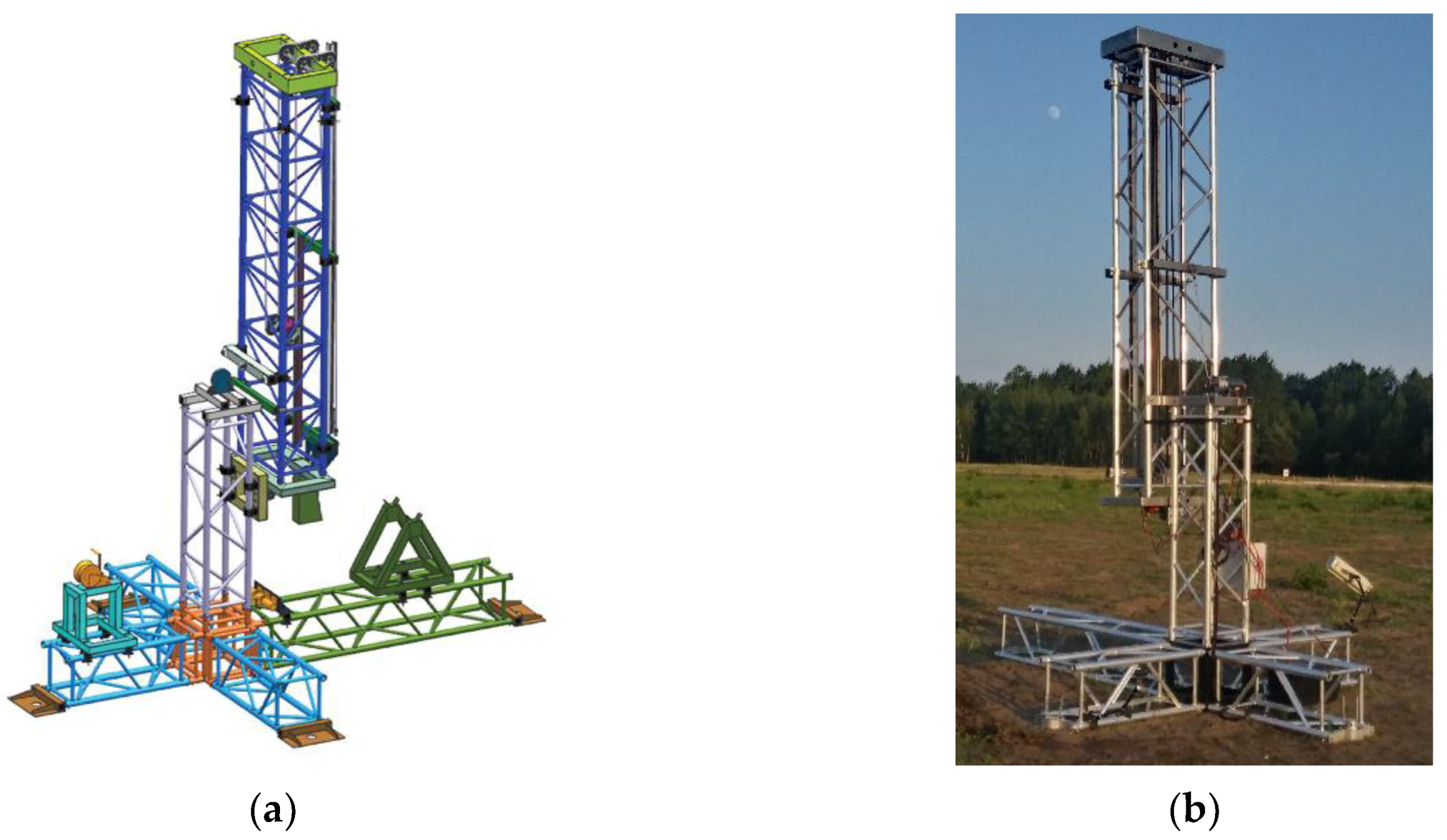
2.2. Test Platform
2.3. Mathematical Model of the Test Platform
2.4. Onboard Instrumentation
2.5. Inertial Measurement Unit Error Model
3. Results
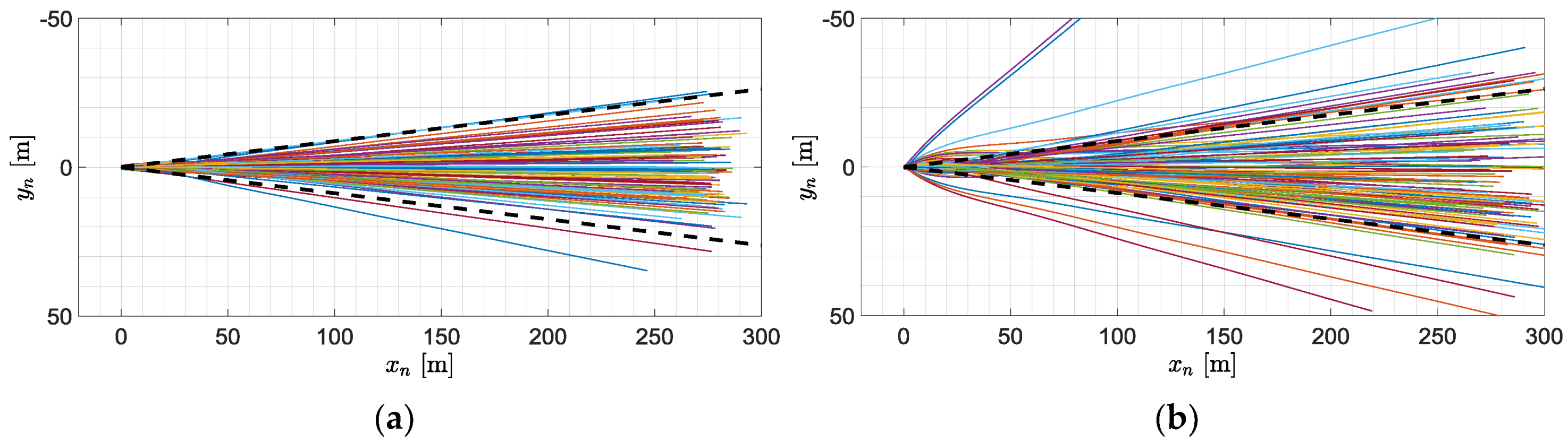
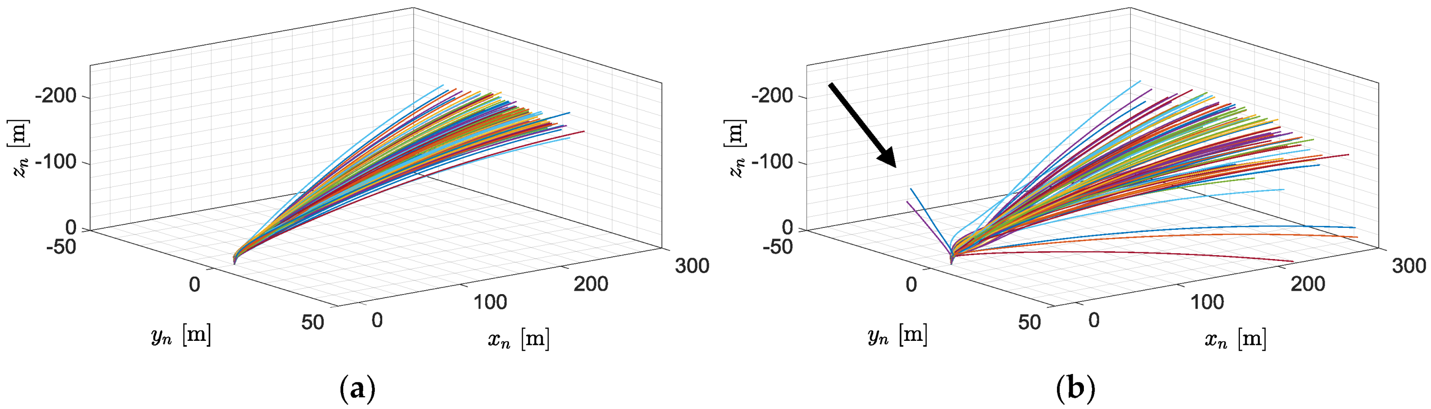
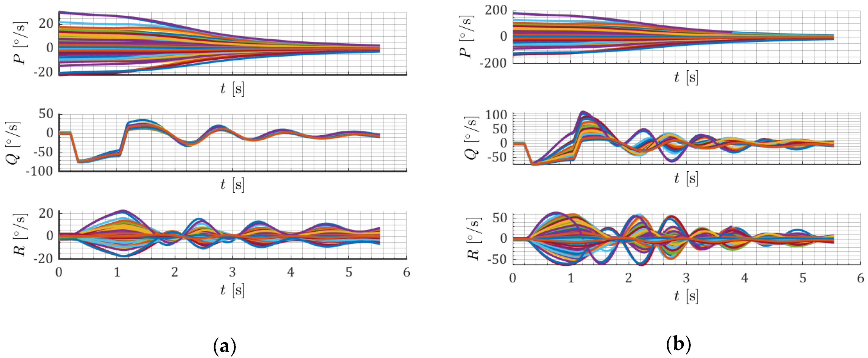
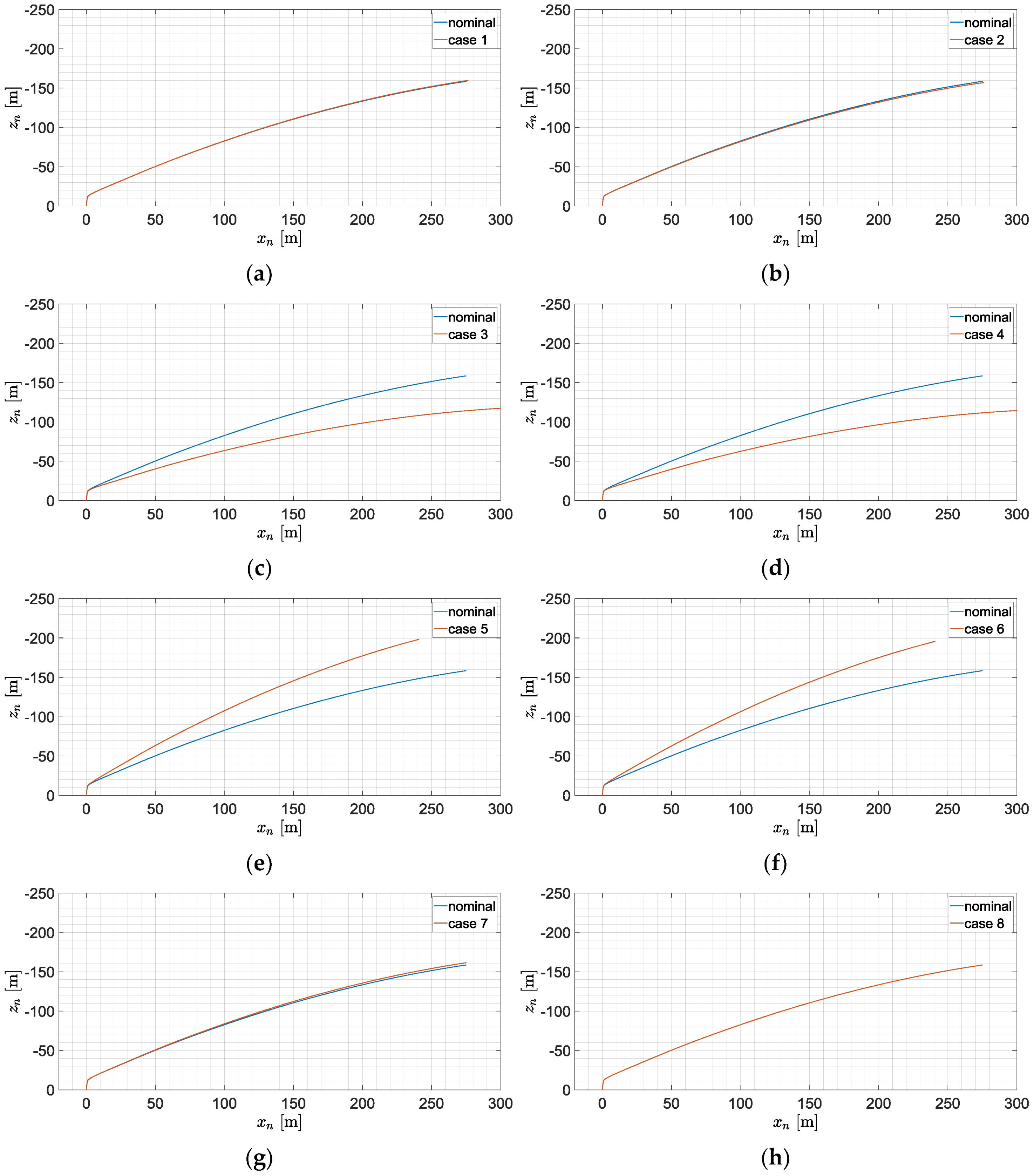
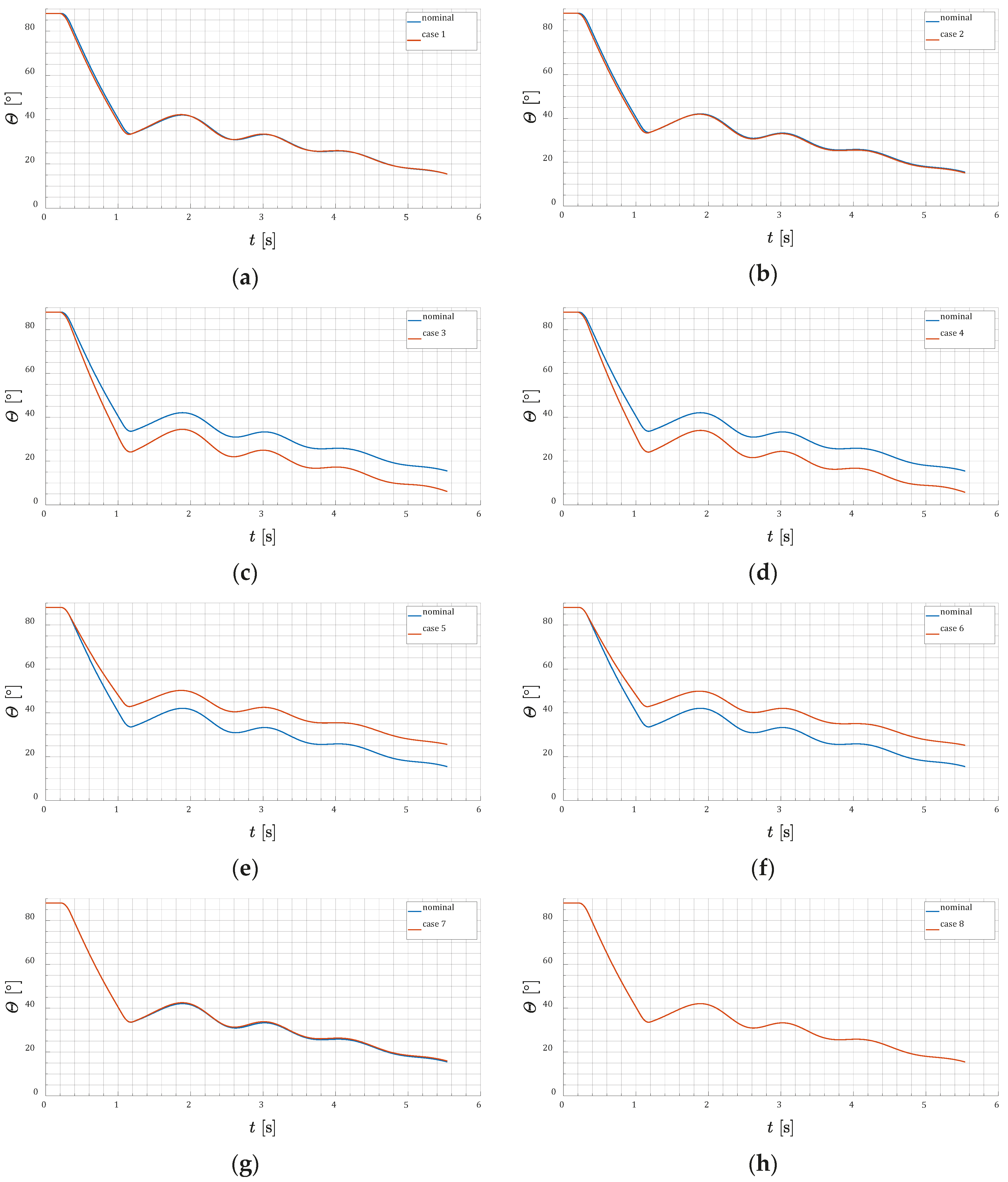
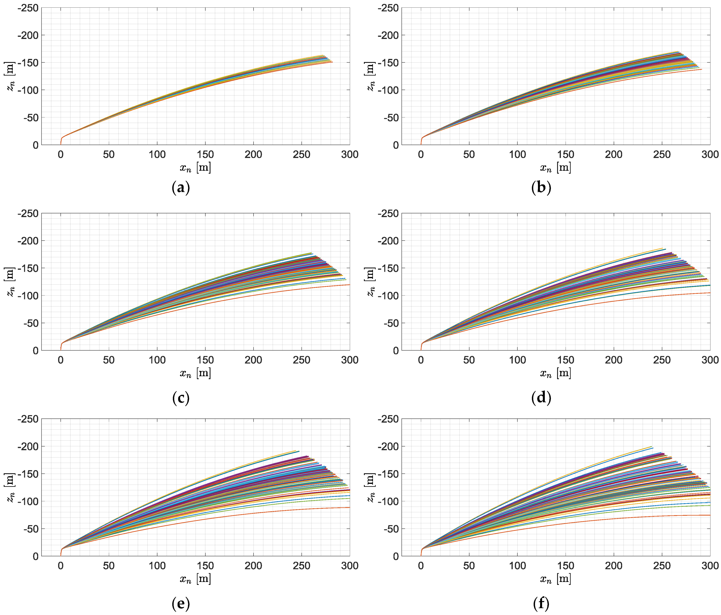
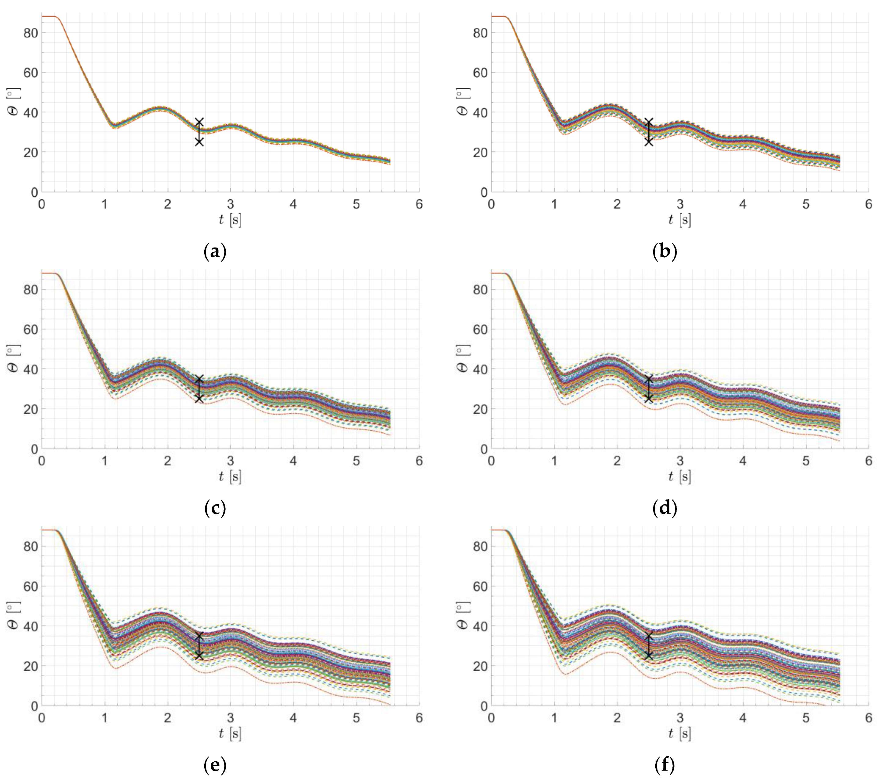
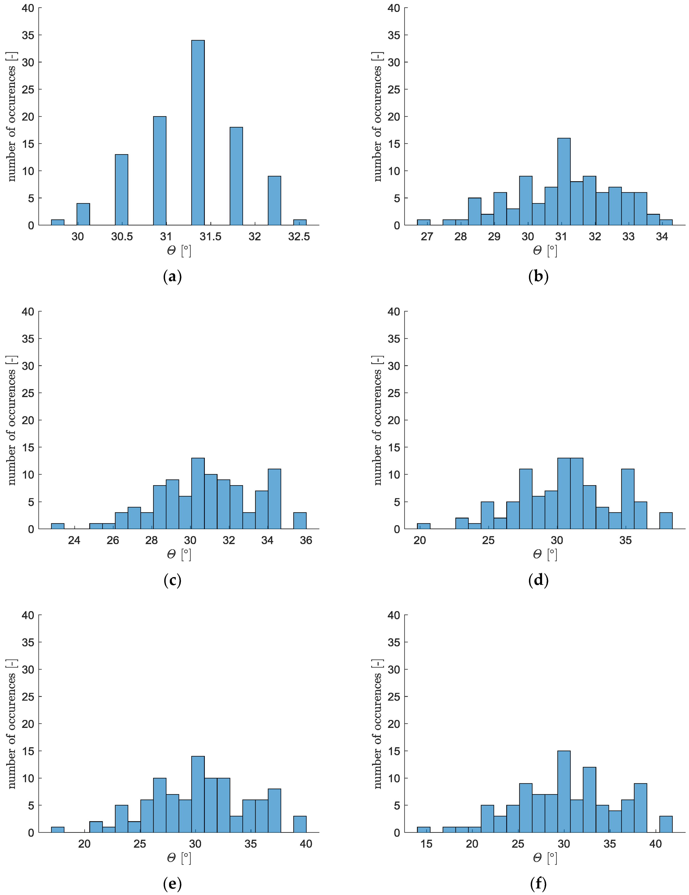
3.1. Monte-Carlo Analysis
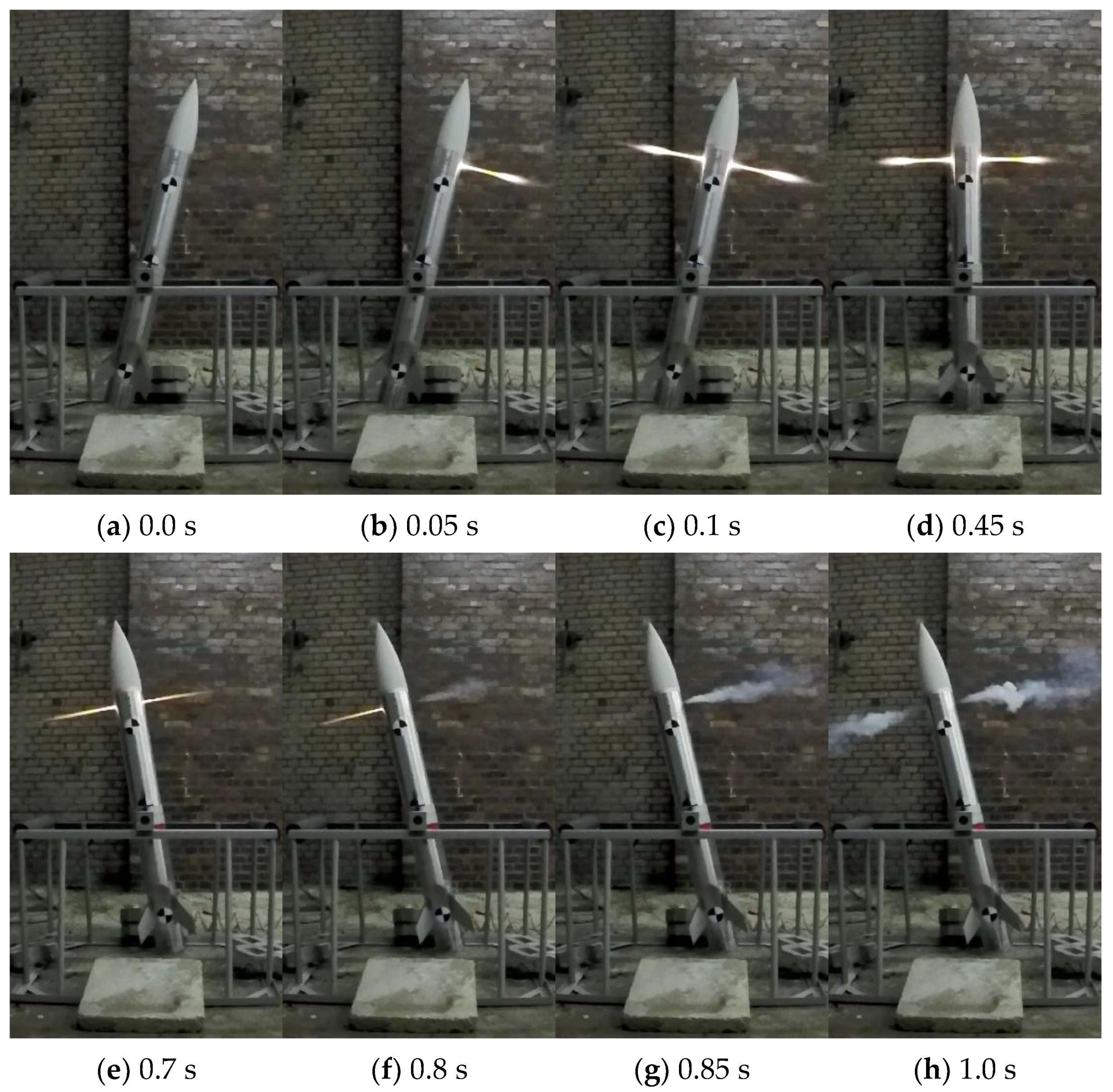
3.2. Ground Tests
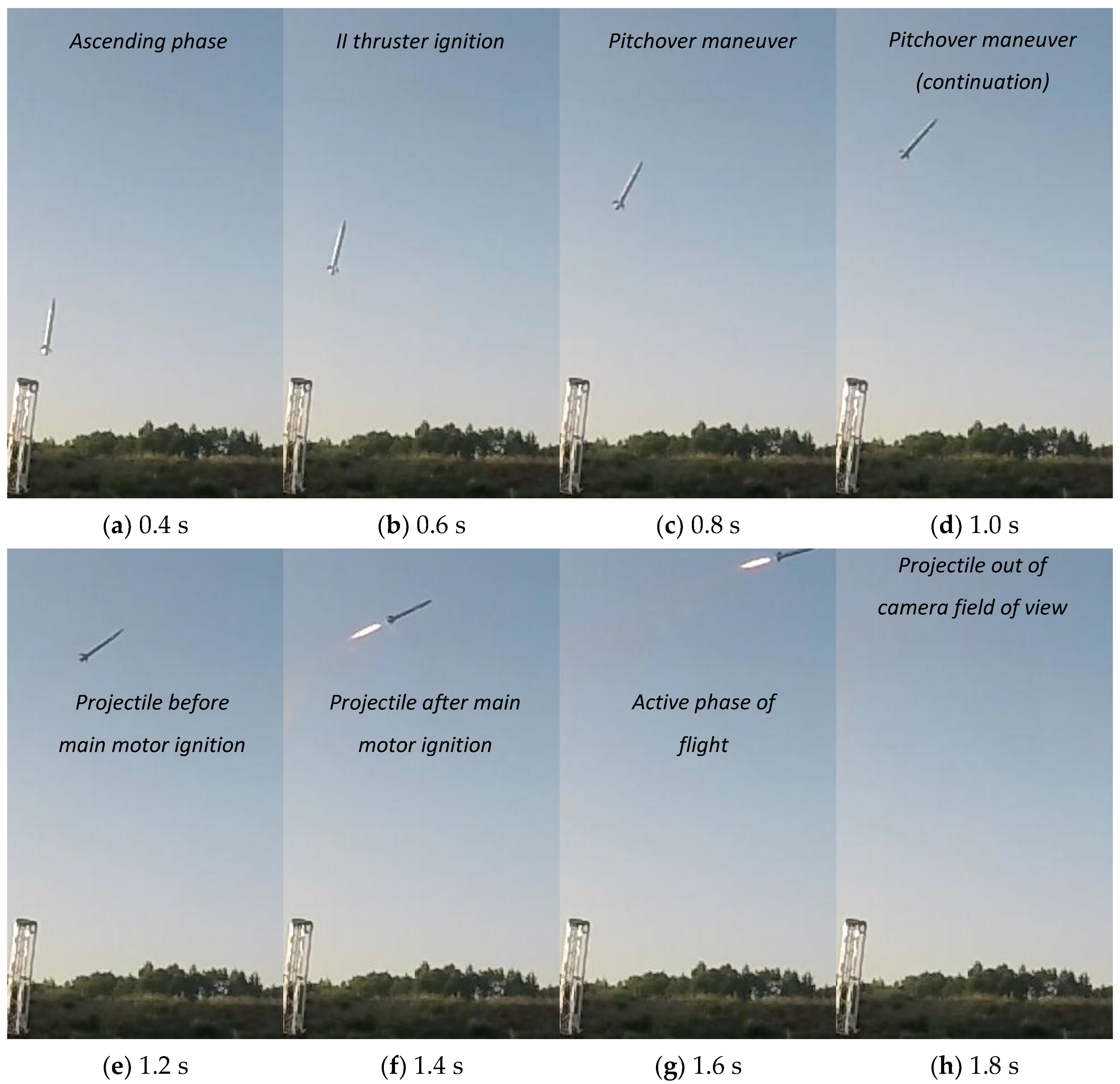
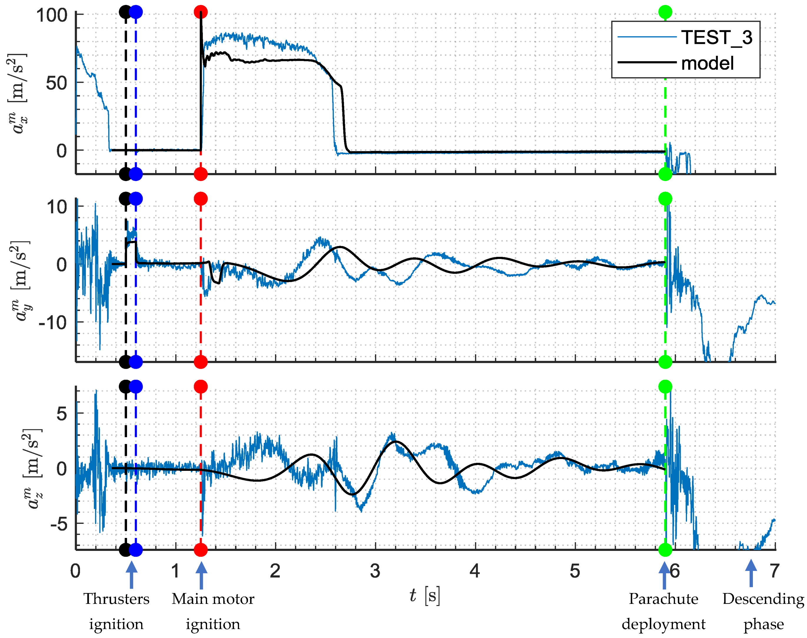
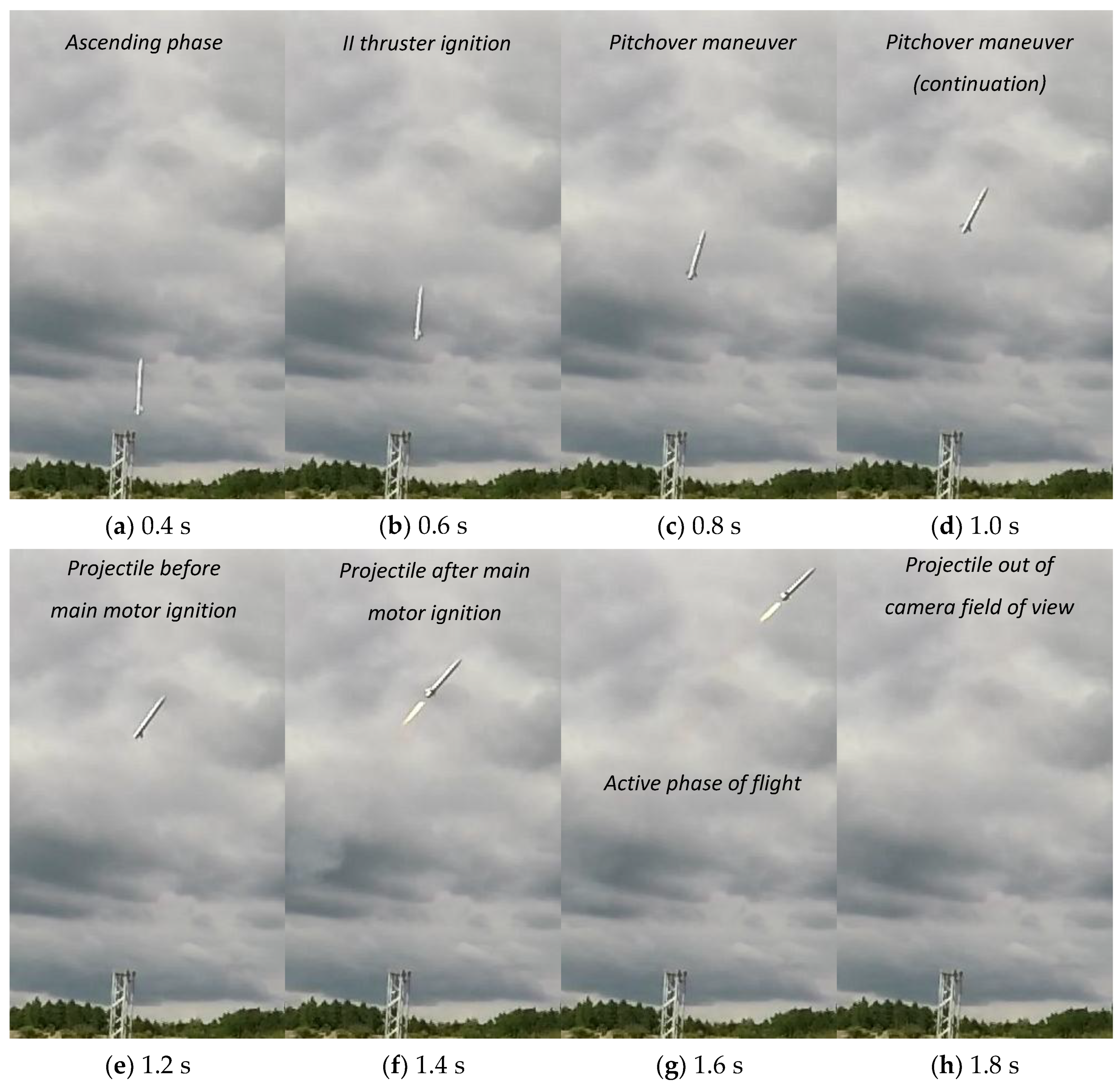
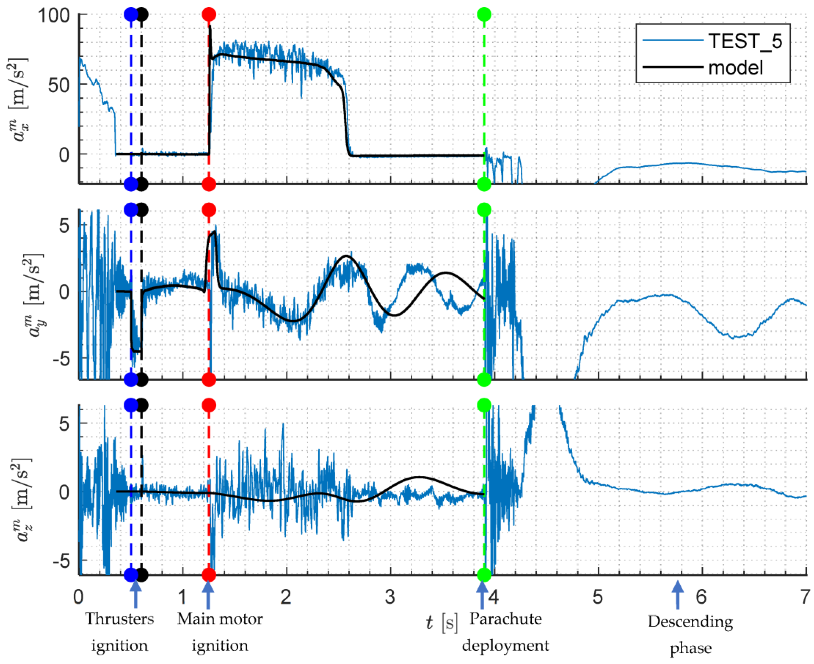
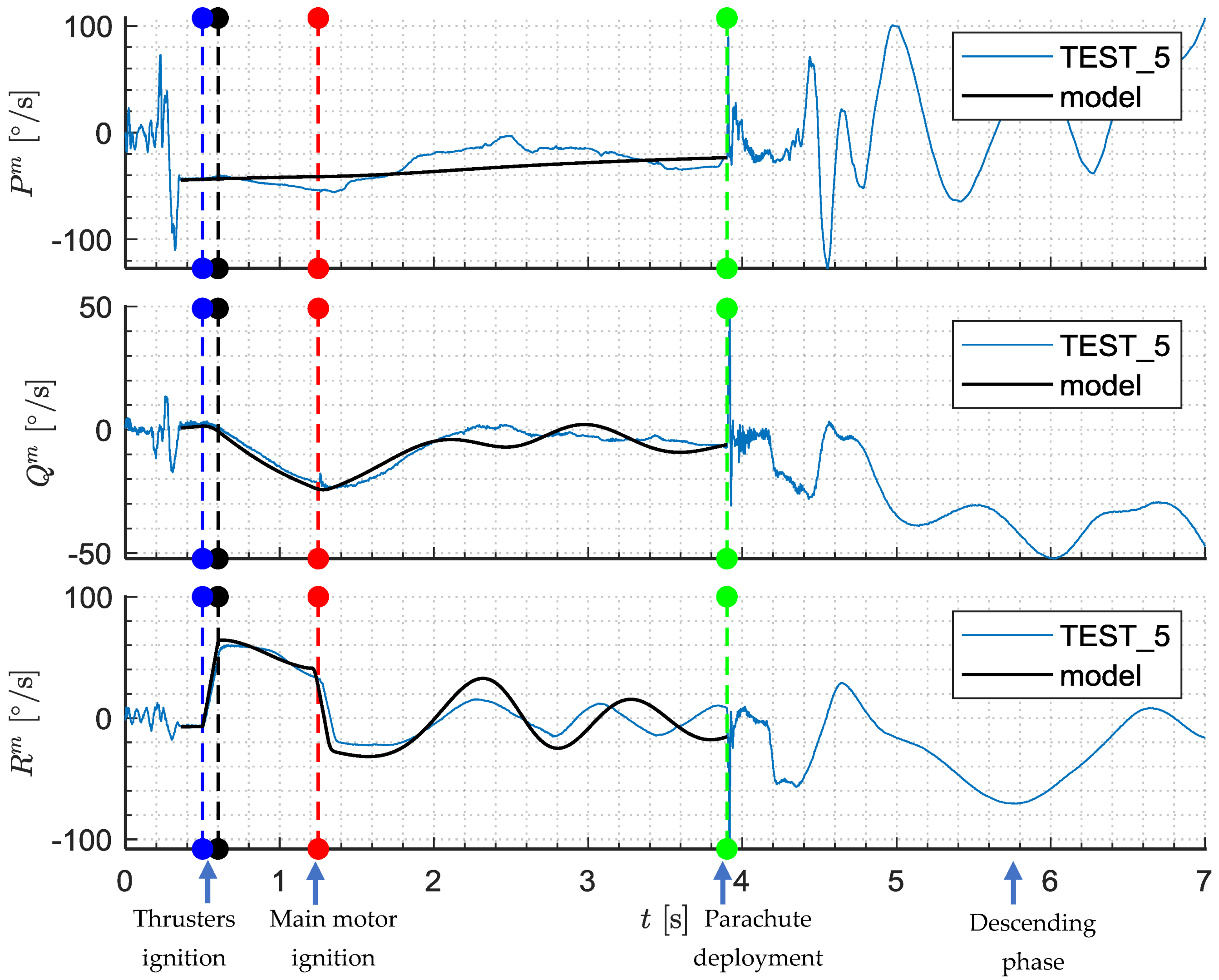
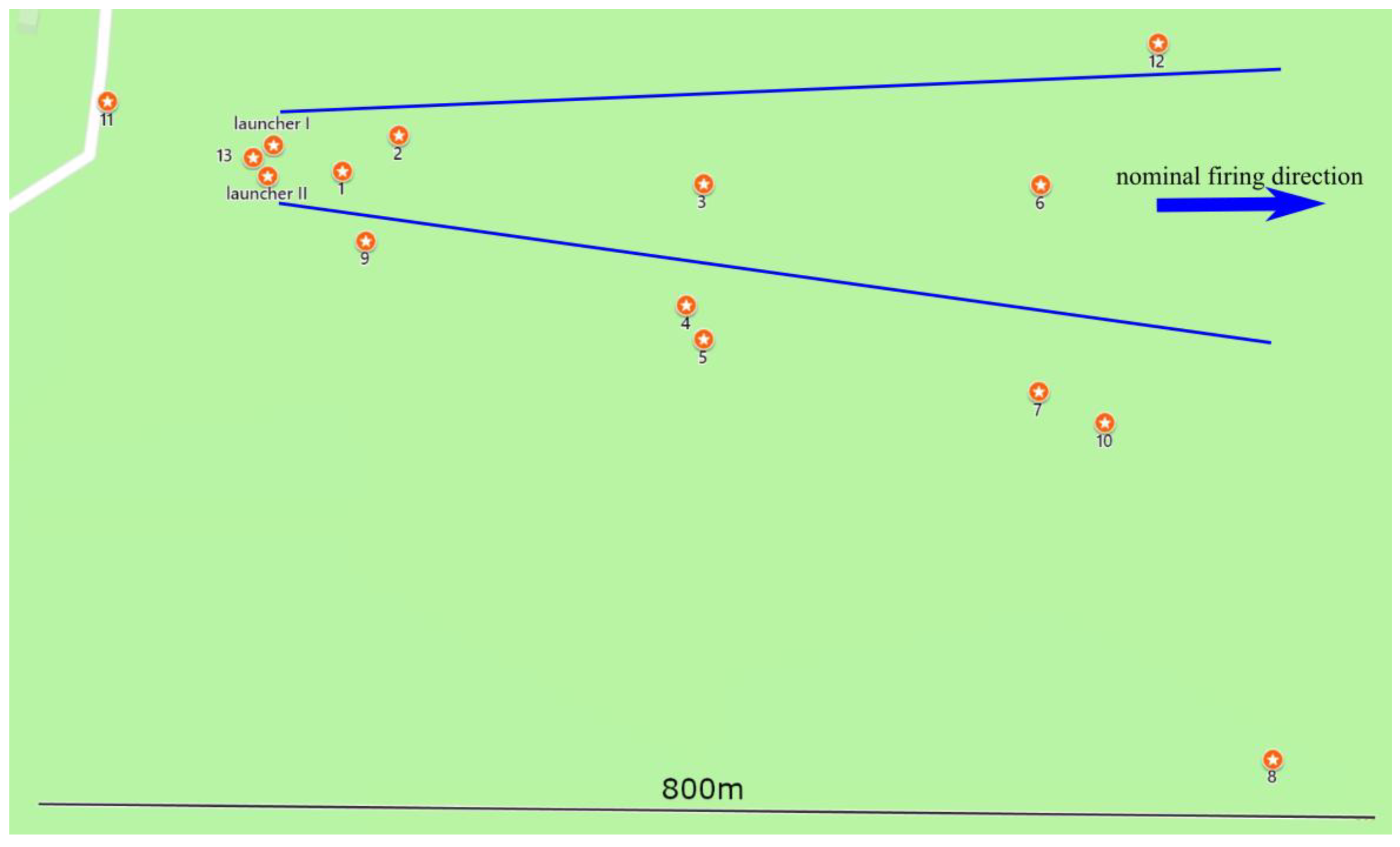
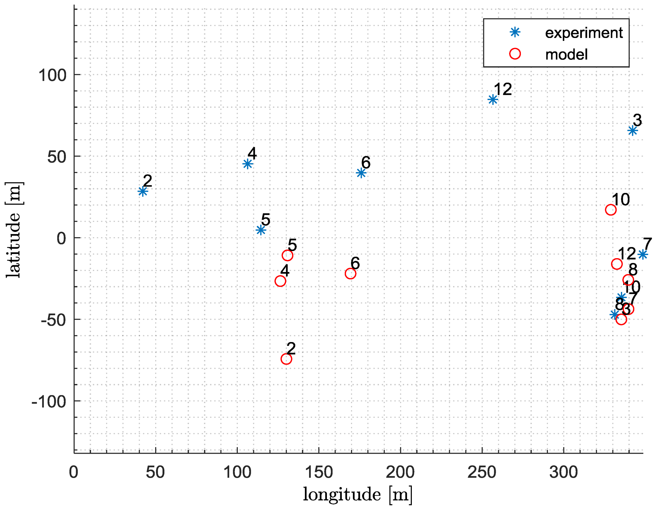
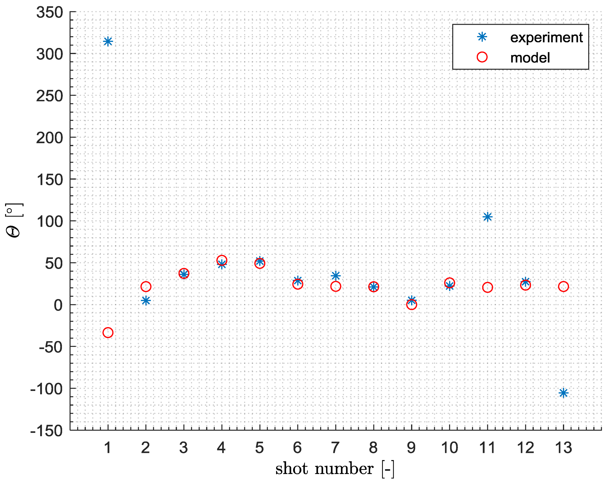
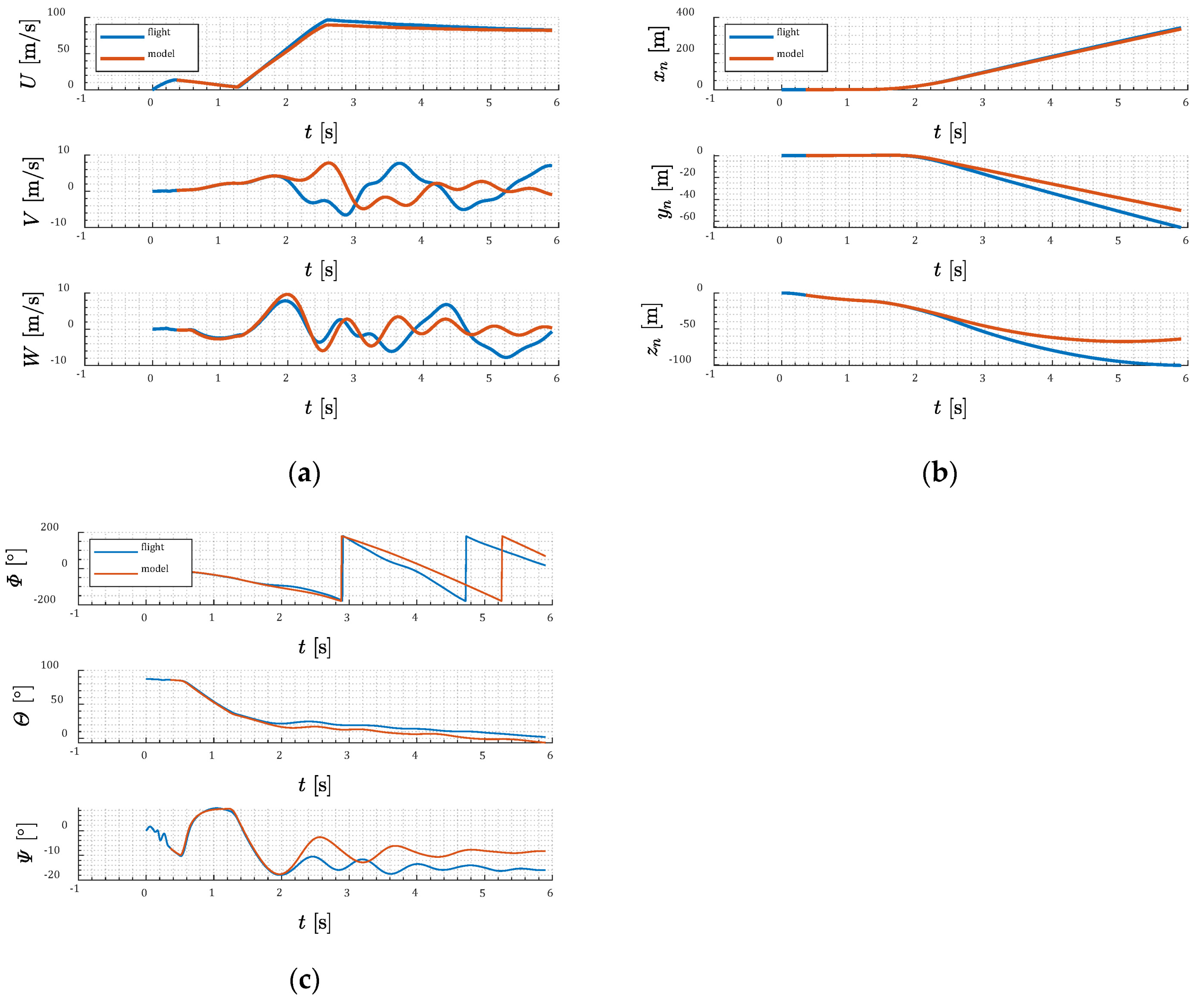
3.3. Flight Tests
4. Conclusions
Author Contributions
Funding
Acknowledgments
Conflicts of Interest
Notation
| Latin symbols | |
| linear accelerations, [m/s2] | |
| linear accelerations measured by IMU, [m/s2] | |
| linear accelerations at IMU location, [m/s2] | |
| bias vector for accelerometers, [m/s2] | |
| bias vector for gyroscopes, [°/s] | |
| bias factors for accelerometers, [m/s2] | |
| bias factors for gyroscopes, [°/s] | |
| rolling, pitching, and yawing moments coefficients, [-] | |
| roll, pitch, and yaw damping moments coefficients, [-] | |
| axial, side, and normal force coefficients, [-] | |
| projectile diameter, [m] | |
| quaternion elements, [-] | |
| quaternion norm, [-] | |
| aerodynamic forces, [N] | |
| total forces in body-fixed frame | |
| gravity forces, [N] | |
| forces generated by lateral thrusters, [N] | |
| forces generated by main motor, [N] | |
| gravity acceleration, [m/s2] | |
| altitude, [m] | |
| numerical integration step, [s] | |
| coefficient which drives the norm of the quaternion state vector to 1.0, [-] | |
| accelerometers scaling matrix, [-] | |
| gyroscopes scaling matrix, [-] | |
| number of the thruster, [-] | |
| inertia matrix, [kgm2] | |
| moments of inertia before main motor burnout, [kgm2] | |
| moments of inertia after main motor burnout, [kgm2] | |
| rolling, pitching, and yawing moment in the body-fixed frame with respect to the center of mass, [Nm] | |
| projectile mass, [kg] | |
| projectile initial mass, [kg] | |
| projectile mass after main motor burnout, [kg] | |
| aerodynamic moments, [Nm] | |
| total moments in body-fixed frame , [Nm] | |
| moments due to gravity, [Nm] | |
| moments due to lateral thrusters, [Nm] | |
| moments due to main motor, [Nm] | |
| number of lateral thrusters, [-] | |
| projectile angular rates in the body-fixed frame , [°/s] | |
| projectile angular rates measured by IMU, [°/s] | |
| vector describing the position of IMU in the body-fixed frame , [m] | |
| scale factors for accelerometers, [-] | |
| scale factors for gyroscopes, [-] | |
| projectile cross section area, [m2] | |
| time, [s] | |
| matrix of transformation from the body-fixed frame to IMU axis, [-] | |
| main motor thrust force, [N] | |
| lateral thruster magnitude, [N] | |
| projectile linear velocities in the body-fixed frame , [m/s] | |
| vector of accelerometers noise, [m/s2] | |
| vector of gyroscopes noise, [°/s] | |
| accelerometers noise, [m/s2] | |
| gyroscopes noise, [°/s] | |
| total flight velocity, [m/s] | |
| the actual center of mass location (from the projectile base), [m] | |
| the initial center of mass location (from the projectile base), [m] | |
| center of mass location after main motor burnout (from the projectile base), [m] | |
| inertial measurement unit location coordinates (from the projectile base), [m] | |
| lateral thruster location coordinate (from the projectile base), [m] | |
| projectile center of mass coordinates in the frame , [m] | |
| axial, side and normal force in the body-fixed frame , [N] | |
| Greek symbols | |
| projectile roll, pitch, and yaw angles, respectively, [°] | |
| IMU enclosure misalignment angles with respect to the body-fixed frame , [°] | |
| pitch misalignment angle of the main motor thrust, [°] | |
| air density, [kg/m3] | |
| first lateral thruster firing time delay, [s] | |
| second lateral thruster firing time delay, [s] | |
| the main motor firing time delay, [s] | |
| yaw misalignment angle of the main motor thrust, [°] | |
| vector of angular rates in the body-fixed frame , [°/s] | |
| Abbreviations | |
| CPU | central processing unit |
| IMU | inertial measurement unit |
| DOF | degree of freedom |
| LSB | least significant bit |
| MEMS | microelectromechanical systems |
References
- Yagla, J.; Anderson, L., Jr. Internal ballistics and missile launch environment for the Vertical Launching System. In Proceedings of the 3rd Joint Thermophysics, Fluids, Plasma and Heat Transfer Conference, St. Louis, MO, USA, 7–11 June 1982. [Google Scholar] [CrossRef]
- Qi, Q.; Chen, Q.; Zhou, Y.; Wang, H.; Zhou, H. Submarine-Launched Cruise Missile Ejecting Launch Simulation and Research. In Proceedings of the 2011 International Conference on Electronic & Mechanical Engineering and Information Technology, Harbin, China, 12–14 August 2011. [Google Scholar] [CrossRef]
- Ma, G.; Chen, F.; Yu, J.; Wang, K.; Jiang, S. Effects of Uncertainties in the Launch Parameters on the Pressure-Equalizing Air Film Around a Vertically Launched Underwater Vehicle. J. Fluids Eng. 2019, 141, 104501. [Google Scholar] [CrossRef]
- Jia-Yi, C.; Chuan-Jing, L.; Ying, C.; Xin, C.; Jie, L. Research on the base cavity of a sub-launched projectile. J. Hydrodynam. 2012, 24, 244–249. [Google Scholar] [CrossRef]
- Wang, Z.L.; Kong, F.S.; Li, H.P. Research on Cylindrical Launcher with Cylindrical Launch Parameters Simulation. Adv. Mat. Res. 2014, 886, 422–425. [Google Scholar] [CrossRef]
- Titchener, P.E.; Veitch, A.J. UK Soft Vertical Launch—A Flexible Solution to an Integral Concept for Ground & Naval Air Defence. In Proceedings of the System Concepts for Integrated Air Defense of Multinational Mobile Crisis Reaction Forces, Valencia, Spain, 22–24 May 2000. [Google Scholar]
- Arkhangelsky, I.I.; Afanasev, P.P.; Golubev, I.S. Design of Guided Anti-Aircraft Missiles (In Russian); Izdatelstva MAI: Moscow, Russia, 2001. [Google Scholar]
- Alberding, M.R.; Ciappi, J.I. Cold—Gas munitions launch system. US Patent US 2008/0148927 A1, 15 July 2008. [Google Scholar]
- Liu, F.; Wang, L. Research on the thrust vector control via jet vane in rapid turning of vertical launch. In Proceedings of the 2013 2nd International Conference on Measurement, Information and Control, Harbin, China, 16–18 August 2013; pp. 837–842. [Google Scholar] [CrossRef]
- Tekin, R.; Ateşoğlu, Ö.; Leblebicioğlu, K. Modeling and Vertical Launch Analysis of an Aero and Thrust Vector Controlled Surface to Air Missile. In Proceedings of the AIAA Atmospheric Flight Mechanics Conference, Toronto, ON, Canada, 2–5 August 2010. [Google Scholar] [CrossRef]
- Zhang, H.; Li, F.; Fan, Y. Design of Vertical Launch Control System for Antiaircraft Missile Using Optical Control. In Proceedings of the 2010 International Conference on Measuring Technology and Mechatronics Automation, Changsha City, China, 13–14 March 2010; pp. 1068–1071. [Google Scholar] [CrossRef]
- Jonsson, H.-O.; Malmberg, G. Optimal Thrust Vector Control for Vertical Launch of Tactical Missiles. J. Guid. Control Dyn. 1982, 5, 17–21. [Google Scholar] [CrossRef]
- Lichota, P.; Jacewicz, M.; Szulczyk, J. Spinning gasodynamic projectile system identification experiment design. Aircr. Eng. Aerosp. Technol. 2020, 92, 452–459. [Google Scholar] [CrossRef]
- Burchett, B. Predictive Optimal Pulse-jet Control for Symmetric Projectiles. In Proceedings of the AIAA Atmospheric Flight Mechanics Conference, National Harbor, MD, USA, 13–17 January 2014. [Google Scholar] [CrossRef]
- Jitpraphai, T.; Costello, M. Dispersion Reduction of a Direct-Fire Rocket Using Lateral Pulse Jets. J. Spacecr. Rocket. 2001, 38, 929–936. [Google Scholar] [CrossRef]
- Burchett, B.T. Genetic Algorithm Optimization of Hydra Pulse Jet Controller. In Proceedings of the AIAA Atmospheric Flight Mechanics Conference and Exhibit, Honolulu, HI, USA, 18–21 August 2008. [Google Scholar] [CrossRef]
- Burchett, B.; Costello, M. Model Predictive Lateral Pulse Jet Control of an Atmospheric Rocket. J. Guid. Control Dyn. 2002, 25, 860–867. [Google Scholar] [CrossRef]
- Taur, D.-R.; Chern, J.-S. Optimal Side Jet Control for Vertically Cold Launched Tactical Missiles. In Proceedings of the AIAA Guidance, Navigation, and Control Conference and Exhibit, Denver, CO, USA, 14–17 August 2000. [Google Scholar] [CrossRef]
- Jacewicz, M.; Głębocki, R. Simulation study of a missile cold launch system. J. Theor. App. Mech-Pol. 2018, 56, 901–913. [Google Scholar] [CrossRef]
- Głębocki, R.; Jacewicz, M. Missile Vertical Launch System with Reaction Control Jets. Issues Armam. Technol. 2018, 145, 25–46. [Google Scholar] [CrossRef]
- Ożóg, R.; Jacewicz, M.; Głębocki, R. Use of Wind Tunnel Measurements Data in Cold Launched Missile Flight Simulations. Measur. Automat. Robot. 2020, 24, 49–60. [Google Scholar] [CrossRef][Green Version]
- Veitch, A.J.; Machell, A.; Winter, J.W.M.; Harriss, R.T. Launching of Missiles. U.S. Patent 7207254B2, 24 April 2007. [Google Scholar]
- Tekin, R.; Atesoglu, O.; Leblebicioglu, K. Flight Control Algorithms for a Vertical Launch Air Defense Missile. In Proceedings of the 2nd EuroGNC 2013 CEAS Specialist Conference on Guidance, Navigation & Control, Delft, The Netherlands, 10–12 April 2013. [Google Scholar] [CrossRef]
- Harriss, R.T. Thruster Pack for Missile Control. GB Patent GB2316663A, 4 March 1998. [Google Scholar]
- Buchanan, G.; Wright, D. The Development of Rocketry Capability in New Zealand—World Record Rocket and First of Its Kind Rocketry Course. Aerospace 2015, 2, 91–117. [Google Scholar] [CrossRef]
- National Aeronautics and Space Administration. U.S. Standard Atmosphere, 1976; National Aeronautics and Space Administration: Washington, DC, USA, 1976.
- Lichota, P.; Szulczyk, J.; Tischler, M.B.; Berger, T. Frequency Responses Identification from Multi-Axis Maneuver with Simultaneous Multisine Inputs. J. Guid. Control Dyn. 2019, 42, 2550–2556. [Google Scholar] [CrossRef]
- Zipfel, P. Modeling and Simulation of Aerospace Vehicle Dynamics; American Institute of Aeronautics and Astronautics, Inc.: Reston, VA, USA, 2000. [Google Scholar]
- Allerton, D. Principles of Flight Simulation; John Wiley & Sons: Wiltshire, UK, 2009. [Google Scholar]
- Cai, G.; Chen, B.M.; Lee, T.H. Unmanned Rotorcraft Systems; Springer: London, UK, 2011. [Google Scholar]
- Military Handbook. Missile Flight Simulation, (Part One), Surface-To-Air Missiles; Technical Report No. MIL-HDBK-1211; Department of Defense: Arlington, VA, USA, 1995.
- Xiao, H.; Li, S.; Shen, Q.; Li, H.; Wang, Q. Automatic Positioning of Spinning Projectile in Trajectory Correction Fuze via GPS/IMU Integration. In Proceedings of the 2007 International Conference on Mechatronics and Automation, Harbin, China, 5–8 August 2007. [Google Scholar] [CrossRef]
- Liu, J.; Zhao, T. In-flight alignment method of navigation system based on microelectromechanical systems sensor measurement. Int. J. Distrib. Sens. N. 2019, 15. [Google Scholar] [CrossRef]
- Xing, H.; Chen, Z.; Yang, H.; Wang, C.; Lin, Z.; Guo, M. Self-Alignment MEMS IMU Method Based on the Rotation Modulation Technique on a Swing Base. Sensors 2018, 18, 1178. [Google Scholar] [CrossRef] [PubMed]
- Analog Devices. Available online: https://www.analog.com/media/en/technical-documentation/data-sheets/adis16448.pdf (accessed on 4 July 2020).
- Fairfax, L.D.; Fresconi, F.E. Position Estimation for Projectiles Using Low-cost Sensors and Flight Dynamics. J. Aerospace Eng. 2012, 27, 611–620. [Google Scholar] [CrossRef]
- Pamadi, K.B.; Ohlmeyer, E.J.; Pepitone, T.R. Assessment of a GPS Guided Spinning Projectile Using an Accelerometer-Only IMU. In Proceedings of the AIAA Guidance, Navigation, and Control Conference and Exhibit, Providence, RI, USA, 16–19 August 2004. [Google Scholar] [CrossRef]
- Liu, F.; Su, Z.; Zhao, H.; Li, Q.; Li, C. Attitude Measurement for High-Spinning Projectile with a Hollow MEMS IMU Consisting of Multiple Accelerometers and Gyros. Sensors 2019, 19, 1799. [Google Scholar] [CrossRef] [PubMed]
- Al-Rawashdeh, Y.M.; Elshafei, M.; Al-Malki, M.F. In-Flight Estimation of Center of Gravity Position Using All-Accelerometers. Sensors 2014, 14, 17567–17585. [Google Scholar] [CrossRef] [PubMed]
- Jekeli, C. Inertial Navigation Systems with Geodetic Applications; Walter de Gruyter: Berlin, Germany, 2001. [Google Scholar]
- Sun, W.; Wang, D.; Xu, L.; Xu, L. MEMS-based rotary strapdown inertial navigation system. Measurement 2013, 46, 2585–2596. [Google Scholar] [CrossRef]
- Groves, P.D. Principles of GNSS, Inertial, and Multisensor Integrated Navigation Systems, 2nd ed.; Artech House: London, UK, 2013. [Google Scholar]
- Pretto, A.; Grisetti, G. Calibration and performance evaluation of low-cost IMUs. In Proceedings of the 20th IMEKO TC4 International Symposium and 18th International Workshop on ADC Modelling and Testing. Research on Electric and Electronic Measurement for the Economic Upturn, Benevento, Italy, 15–17 September 2014. [Google Scholar]
- Britting, K.R. Inertial Navigation Systems Analysis; John Wiley & Sons, Inc.: New York, NY, USA, 1971. [Google Scholar]
- Andreev, V.D. Theory of Inertial Navigation Aided Systems; Izdatelstva Nauka: Moscow, Russia, 1967. (In Russian) [Google Scholar]
- Titterton, D.H.; Weston, J.L. Strapdown Inertial Navigation Technology, 2nd ed.; The Institution of Electrical Engineers: London, UK, 2004. [Google Scholar]
- Ilg, M. Multi-Core Computing Cluster for Safety Fan Analysis of Guided Projectiles; Army Research Laboratory: Aberdeen Proving Ground, MD, USA, 2011. [Google Scholar]
- Ilg, M. Guidance, Navigation, and Control System Simulations via Graphics Processor Unit; Army Research Laboratory: Aberdeen Proving Ground, MD, USA, 2011. [Google Scholar]
- Ilg, M.; Rogers, J.; Costello, M. Projectile Monte-Carlo Trajectory Analysis Using a Graphics Processing Unit. In Proceedings of the AIAA Atmospheric Flight Mechanics Conference, Portland, OR, USA, 8–11 August 2011. [Google Scholar] [CrossRef]
- Matsumoto, M.; Nishimura, T. Mersenne twister: A 623-dimensionally equidistributed uniform pseudo-random number generator. ACM Trans. Model. Comput. Simul. 1998, 8, 3–30. [Google Scholar] [CrossRef]
- Lichota, P.; Szulczyk, J.; Noreña, D.A.; Vallejo Monsalve, F.A. Power spectrum optimization in the design of multisine manoeuvre for identification purposes. J. Theor. App. Mech-Pol. 2017, 55, 1193–1203. [Google Scholar] [CrossRef]


| No. | Parameter | Mean Value | Standard Deviation | Unit |
|---|---|---|---|---|
| 1 | 15.97 | 0.05 | kg | |
| 2 | 15.24 | 0.05 | kg | |
| 3 | 0.057 | 0.01 | kgm2 | |
| 4 | 0.056 | 0.01 | kgm2 | |
| 5 | = | 3.617 | 0.01 | kgm2 |
| 6 | = | 3.458 | 0.01 | kgm2 |
| 7 | 17 | 1 | m/s | |
| 8 | 0 | 0.1 | m/s | |
| 9 | 0 | 0.1 | m/s | |
| 10 | 0 | 10/20/30/40/50/60 | °/s | |
| 11 | 0 | 1 | °/s | |
| 12 | 0 | 1 | °/s | |
| 13 | 0 | 0.02 | m | |
| 14 | 0 | 0.02 | m | |
| 15 | 0 | 0.02 | m | |
| 16 | 0 | 0.2 | ° | |
| 17 | 88 | 0.1 | ° | |
| 18 | 0 | 0.1 | ° | |
| 19 | 0 | 0.01 | ° | |
| 20 | 0 | 0.01 | ° |
| Case No. | |||
|---|---|---|---|
| 1 | 0.2 − 0.011 | 0.33 − 0.011 | 0.95 − 0.011 |
| 2 | 0.2 − 0.011 | 0.33 − 0.011 | 0.95 + 0.011 |
| 3 | 0.2 − 0.011 | 0.33 + 0.011 | 0.95 − 0.011 |
| 4 | 0.2 − 0.011 | 0.33 + 0.011 | 0.95 + 0.011 |
| 5 | 0.2 + 0.011 | 0.33 − 0.011 | 0.95 − 0.011 |
| 6 | 0.2 + 0.011 | 0.33 − 0.011 | 0.95 + 0.011 |
| 7 | 0.2 + 0.011 | 0.33 + 0.011 | 0.95 − 0.011 |
| 8 | 0.2 + 0.011 | 0.33 + 0.011 | 0.95 + 0.011 |
| No. | Parameter | Mean Value [s] | Standard Deviation [s] |
|---|---|---|---|
| 1 | 0.2 | 0.001/0.003/0.005/0.007/0.009/0.011 | |
| 2 | 0.33 | 0.001/0.003/0.005/0.007/0.009/0.011 | |
| 3 | 0.95 | 0.001/0.003/0.005/0.007/0.009/0.011 |
| Test No. | Ignition Delay [s] | Initial Angle 1 [°] | Final Angle 2 [°] | Total Angle [°] |
|---|---|---|---|---|
| 1 | 0.050 | −13.97 | 12.55 | 26.52 |
| 2 | 0.10 | −8.09 | 43.98 | 52.07 |
| 3 | 0.125 | −13.92 | 39.64 | 53.56 |
| 4 | 0.150 | −10.41 | 54.15 | 64.56 |
| Flight Number | 1 | 2 | 3 | 4 | 5 | 6 | 7 | 8 | 9 | 10 | 11 | 12 | 13 | |
|---|---|---|---|---|---|---|---|---|---|---|---|---|---|---|
| Date (YYYY-MM-DD)/Time (hh-mm) | 2019-06-14/ 14:37 UTC | 2019-06-14/ 16:26 UTC | 2019-06-14/ 17:34 UTC | 2019-06-17/ 12:55 UTC | 2019-06-17/ 13:35 UTC | 2019-06-17/ 14:16 UTC | 2019-06-17/ 15:45 UTC | 2019-07-05/ 07:35 UTC | 2019-07-05/ 07:56 UTC | 2019-07-05/ 09:22 UTC | 2019-07-05/ 09:37 UTC | 2019-07-05/ 10:03 UTC | 2019-07-05/ 10:18 UTC | |
| Thrusters Location: 1 | Forward | Forward | Forward | Aft | Aft | Aft | Aft | Aft | Aft | Forward | Forward | Forward | Forward | |
| Time from launch: | I thruster firing [ms]: | 500 | 500 | 500 | 600 | 600 | 650 | 650 | 650 | 650 | 500 | 500 | 500 | 500 |
| II thruster firing [ms]: | 650 | 650 | 600 | 500 | 500 | 500 | 500 | 500 | 500 | 650 | 650 | 650 | 650 | |
| Main motor firing [ms]: | 1500 | 1500 | 1250 | 1250 | 1250 | 1300 | 1300 | 1300 | 1300 | 1300 | 1300 | 1300 | 1500 | |
| Parachute deployment [ms]: | 5900 | 5900 | 5900 | 3900 | 3900 | 3900 | 5900 | 5900 | 5900 | 5900 | 5900 | 5900 | 5900 | |
| Nominal pitch angle [°]: 2 | 30 | 30 | 45 | 45 | 45 | 30 | 30 | 30 | 30 | 30 | 30 | 30 | 30 | |
| Projectile position after landing [°]: 3 | 52.303128N | 52.303318N | 52.303054N | 52.302400N | 52.302217N | 52.303050N | 52.301933N | 52.299944N | 52.302750N | 52.301767N | 52.303500N | 52.303817N | 52.303200N | |
| 21.187892E | 21.188386E | 21.191082E | 21.190933E | 21.191083E | 21.194067E | 21.194050E | 21.196115E | 21.188100E | 21.194633E | 21.185817E | 21.195100E | 21.187100E | ||
| Projectile position after landing [m]: 4 | −15.801 | 5.341 | −24.035 | −96.808 | −117.171 | −24.480 | −148.772 | −370.094 | −57.862 | −167.243 | 25.593 | 60.866 | −7.789 | |
| 41.746 | 75.444 | 259.346 | 249.182 | 259.414 | 462.961 | 461.802 | 602.661 | 55.935 | 501.570 | −99.796 | 533.425 | −12.278 | ||
| Projectile position at parachute deployment [m]: 4 | 16.877 | 42.141 | 342.200 | 106.360 | 114.454 | 175.929 | 348.414 | 331.275 | Lack of data | 335.353 | −46.861 | 256.588 | −5.868 | |
| −12.596 | 28.442 | 65.681 | 45.259 | 4.752 | 39.715 | −10.209 | −47.069 | Lack of data | −36.507 | −1.116 | 84.695 | 0.283 | ||
| Results: | Negative | Partially positive | Positive | Positive | Positive | Positive | Positive | Positive | Partially positive | Positive | Partially positive | Positive | Negative | |
| Flight Number | 2 | 3 | 4 | 5 | 6 | 7 | 8 | 10 | 12 |
|---|---|---|---|---|---|---|---|---|---|
| Mean error | |||||||||
| [m] | −0.2488 | −0.0188 | −0.0312 | −0.0316 | −0.0373 | −0.0545 | −0.0332 | −0.0592 | −0.2014 |
| [m] | −0.2059 | −0.0214 | −0.0662 | −0.0169 | −0.0521 | −0.0291 | 0.0302 | 0.0008 | −0.0829 |
| [m] | −0.3307 | −0.0015 | 0.0120 | 0.0148 | 0.0036 | −0.0141 | −0.0036 | −0.0171 | −1.1704 |
| [°] | 7.1416 | 0.8765 | 6.9302 | −2.2923 | −0.4534 | −0.9227 | −3.6369 | −0.1954 | 6.4360 |
| [°] | 0.9950 | −1.0482 | −0.5608 | −1.4967 | −1.7322 | −4.6415 | −3.6441 | −2.7312 | −4.8897 |
| [°] | 5.5798 | 0.2315 | 6.6055 | −2.5187 | 0.0964 | −1.0370 | −0.3300 | 1.0658 | −0.4549 |
| 90th percentile | |||||||||
| [m] | 0.4161 | 0.0468 | 0.0826 | 0.0705 | 0.0760 | 0.1319 | 0.0716 | 0.1450 | 0.2920 |
| [m] | 0.3939 | 0.0465 | 0.1660 | 0.0441 | 0.1242 | 0.0748 | 0.0734 | 0.0045 | 0.1054 |
| [m] | 0.5889 | 0.0067 | 0.0295 | 0.0335 | 0.0078 | 0.0327 | 0.0227 | 0.0425 | 1.8304 |
| [°] | 12.2989 | 1.4353 | 13.6337 | 4.2564 | 2.1060 | 2.0032 | 9.6460 | 1.3444 | 17.6549 |
| [°] | 4.4989 | 1.5623 | 1.3480 | 2.7248 | 2.8874 | 9.0548 | 6.6079 | 5.0795 | 10.5973 |
| [°] | 12.1665 | 1.1023 | 13.2632 | 4.1704 | 2.2862 | 1.9113 | 1.3250 | 1.5504 | 1.3854 |
| Flight Number | 2 | 3 | 4 | 5 | 6 | 7 | 8 | 10 | 12 |
|---|---|---|---|---|---|---|---|---|---|
| Mean error | |||||||||
| [m] | −0.1847 | −3.5012 | 6.6953 | 6.5349 | −2.3807 | −3.6740 | 4.4036 | −1.6894 | 34.3138 |
| [m] | 1.9534 | 6.7380 | 6.5140 | −2.5694 | 5.8000 | −23.0947 | −30.6974 | −7.8907 | 29.4633 |
| [m] | −4.6852 | 14.8725 | 6.2747 | −0.7169 | −2.3809 | 25.8254 | 19.0830 | 15.4702 | 15.5533 |
| [°] | −1.5164 | −5.1513 | −43.4231 | −7.8804 | 9.6307 | −9.8136 | −21.4121 | −18.1197 | 58.5144 |
| [°] | 14.3996 | −6.5306 | −8.7469 | −5.7552 | 1.8439 | −10.3835 | −9.7991 | −7.6187 | −15.3859 |
| [°] | 12.2608 | 5.0300 | 17.3938 | 0.1760 | 7.2533 | −7.0502 | −13.6167 | −5.4303 | 13.2285 |
| 90th percentile | |||||||||
| [m] | 1.0338 | 6.5893 | 17.0451 | 14.2016 | 5.6614 | 7.8568 | 7.3294 | 5.5473 | 67.5822 |
| [m] | 5.9457 | 14.0069 | 16.0941 | 5.3563 | 15.1916 | 47.4902 | 64.3578 | 17.0308 | 60.6868 |
| [m] | 10.8209 | 32.2830 | 16.4532 | 1.3357 | 5.1362 | 54.6102 | 40.2059 | 33.3072 | 36.9491 |
| [°] | 66.5019 | 268.9701 | 28.4429 | 18.2725 | 226.1356 | 109.3345 | 41.3030 | 113.8990 | 87.9003 |
| [°] | 19.8762 | 8.7405 | 12.6294 | 8.3592 | 5.9208 | 14.2330 | 11.9204 | 10.2717 | 18.1685 |
| [°] | 18.9189 | 9.3504 | 23.2817 | 4.4185 | 11.6549 | 8.8623 | 16.8968 | 7.4314 | 19.0809 |
Publisher’s Note: MDPI stays neutral with regard to jurisdictional claims in published maps and institutional affiliations. |
© 2020 by the authors. Licensee MDPI, Basel, Switzerland. This article is an open access article distributed under the terms and conditions of the Creative Commons Attribution (CC BY) license (http://creativecommons.org/licenses/by/4.0/).
Share and Cite
Głębocki, R.; Jacewicz, M. Sensitivity Analysis and Flight Tests Results for a Vertical Cold Launch Missile System. Aerospace 2020, 7, 168. https://doi.org/10.3390/aerospace7120168
Głębocki R, Jacewicz M. Sensitivity Analysis and Flight Tests Results for a Vertical Cold Launch Missile System. Aerospace. 2020; 7(12):168. https://doi.org/10.3390/aerospace7120168
Chicago/Turabian StyleGłębocki, Robert, and Mariusz Jacewicz. 2020. "Sensitivity Analysis and Flight Tests Results for a Vertical Cold Launch Missile System" Aerospace 7, no. 12: 168. https://doi.org/10.3390/aerospace7120168
APA StyleGłębocki, R., & Jacewicz, M. (2020). Sensitivity Analysis and Flight Tests Results for a Vertical Cold Launch Missile System. Aerospace, 7(12), 168. https://doi.org/10.3390/aerospace7120168