Impact of Hybrid-Electric Aircraft on Contrail Coverage


Abstract
:1. Introduction
2. Methodology
2.1. The Base Model EMAC
2.2. The CONTRAIL Submodel
2.3. The HEA Extended Schmidt–Appleman Criterion
3. Results
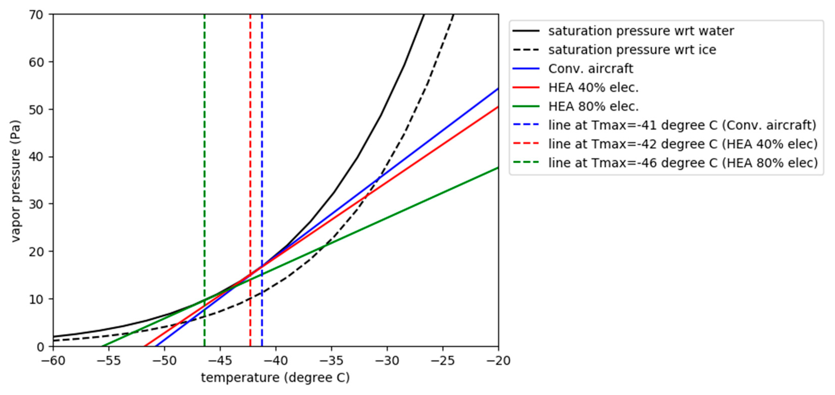
3.1. The Threshold of Contrail Formation Calculated by SAC
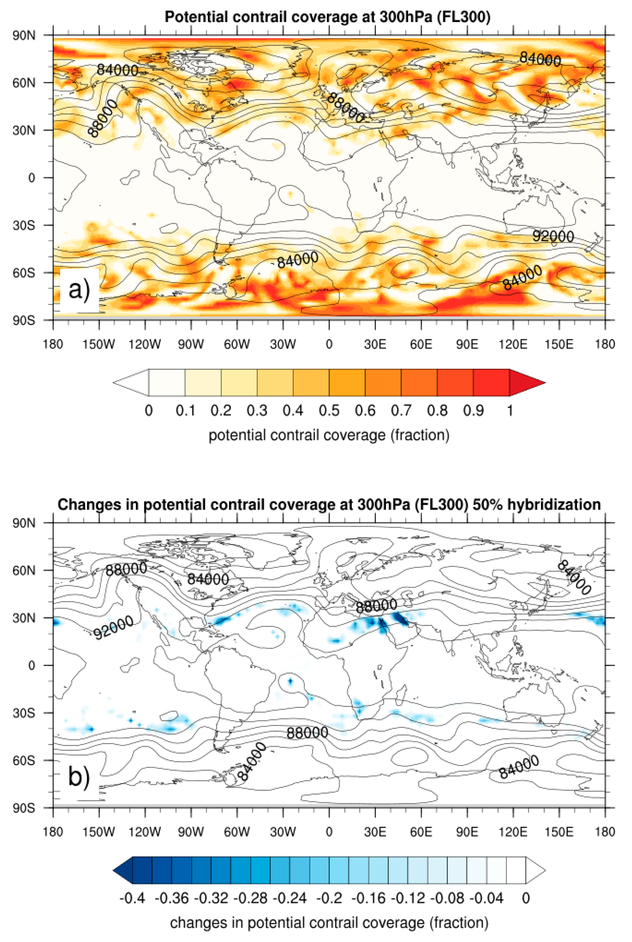
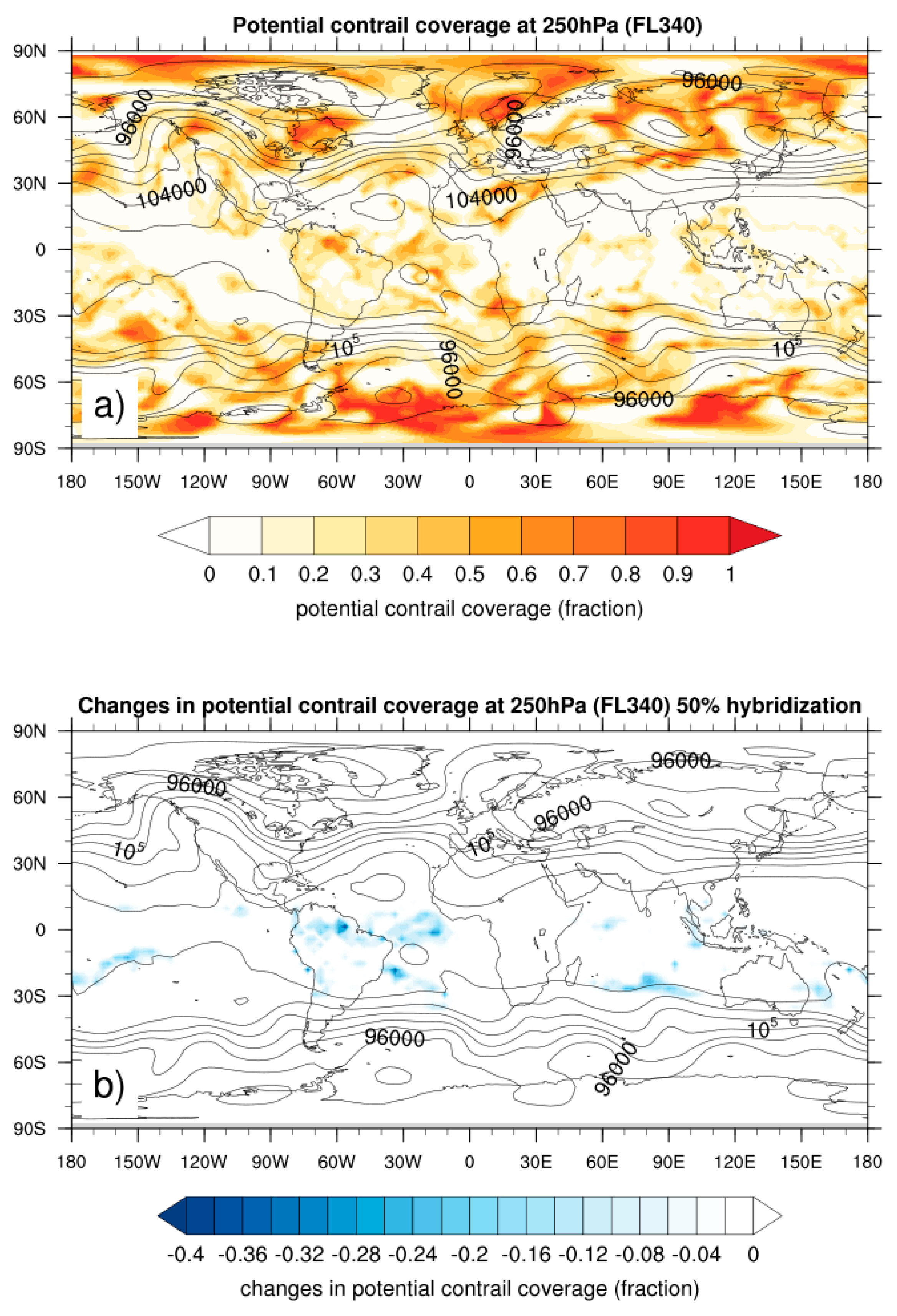
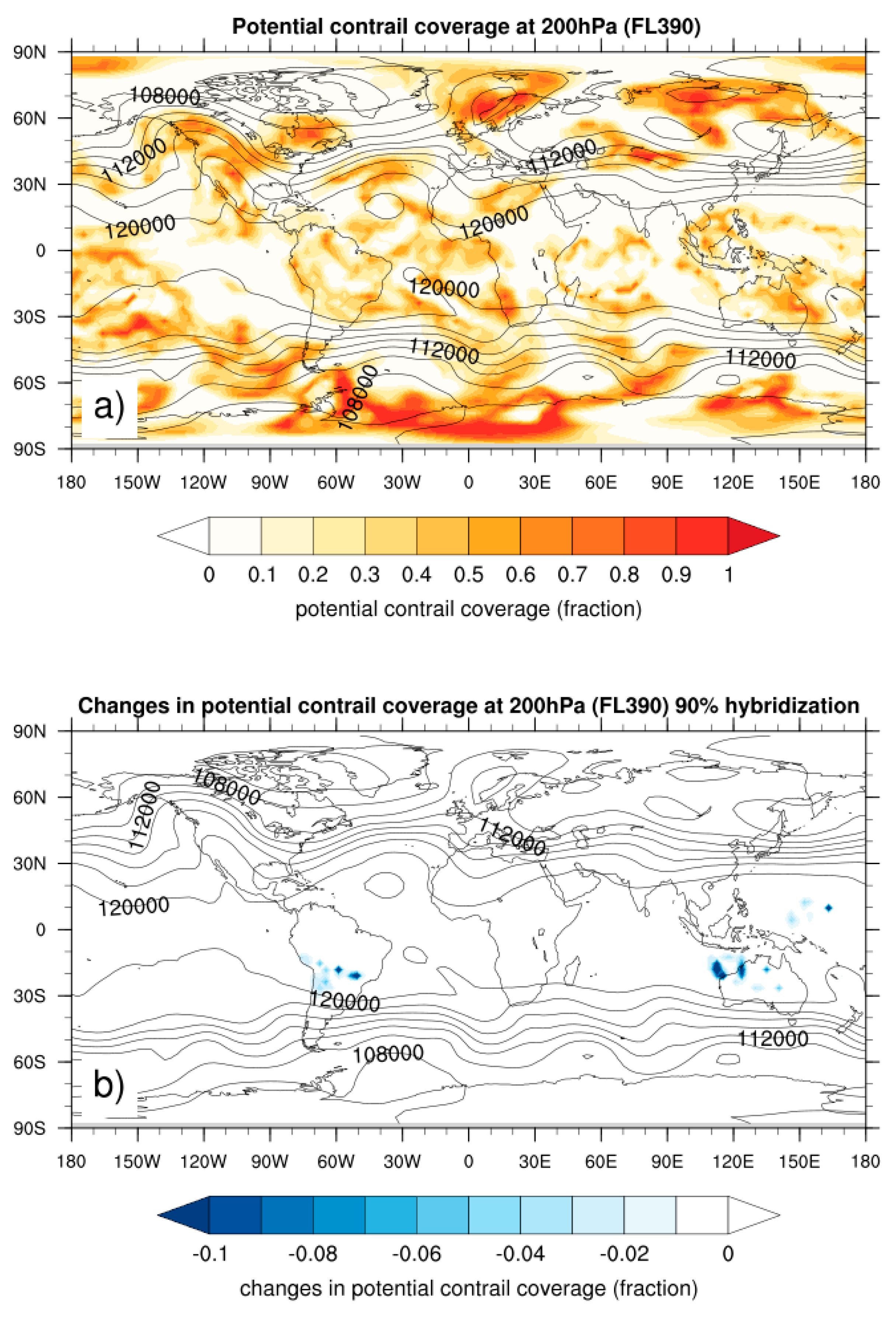
3.2. Changes in Potential Contrail Coverage
3.2.1. One-Day Case Study
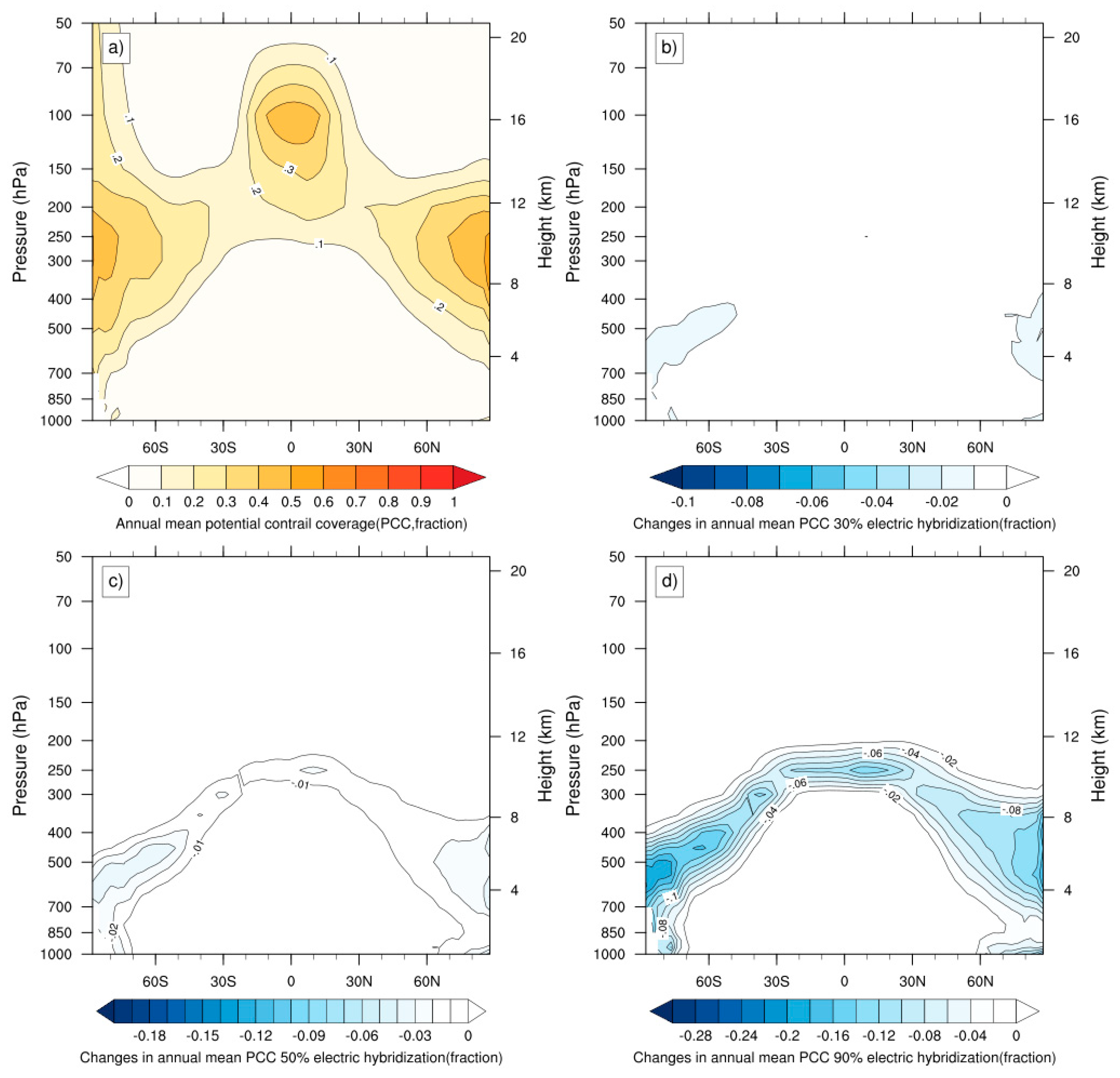
3.2.2. Effect of Degree of Hybridization
3.2.3. Climatology of Contrail Formation
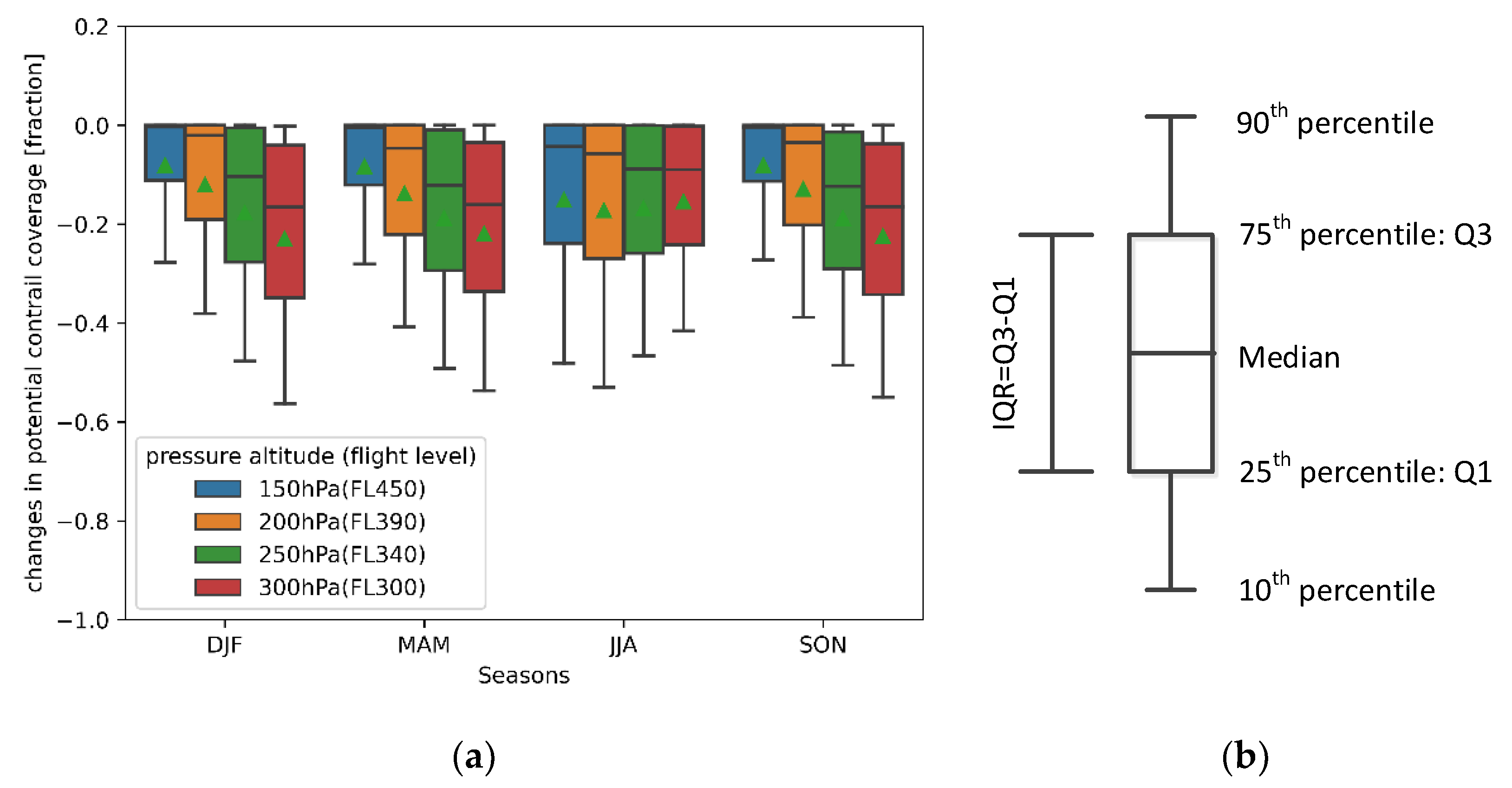
3.2.4. Seasonal Effects
4. Discussion
5. Conclusions
- The atmospheric areas of contrail formation of hybrid-electric aircraft are smaller than those of conventional aircraft and require lower atmospheric temperatures.
- The reduction in contrail formation by hybrid-electric aircraft is more pronounced in a tropical region where the temperatures are higher.
- With a small degree of hybridization (below 30% in the current study), the contrail coverage remains nearly unchanged. A maximum reduction of about 40% in contrail coverage was observed locally, with 90% electric power in use.
- In non-summer, the reduction in potential contrail coverage by hybrid-electric aircraft was more noticeable at lower flight altitudes. In contrast, the changes in potential contrail coverage were nearly constant (about 20%) for all flight altitudes studied in summer.
Author Contributions
Funding
Conflicts of Interest
Nomenclature
| Abbreviations | ||
| DJF | December, January, and February | |
| EIH2O | Water vapor emission index | kg/kg(fuel) |
| EM | Electric motor | |
| HEA | Hybrid-electric aircraft | |
| JJA | June, July, and August | |
| MAM | March, April, and May | |
| PCC | Potential contrail coverage | |
| Probability density function | ||
| RF | Radiative forcing | |
| SAC | Schmidt–Appleman criterion | |
| SON | September, October, and November | |
| Symbols | ||
| Isobaric heat capacity of the air | J/kg/K | |
| F | Thrust | N |
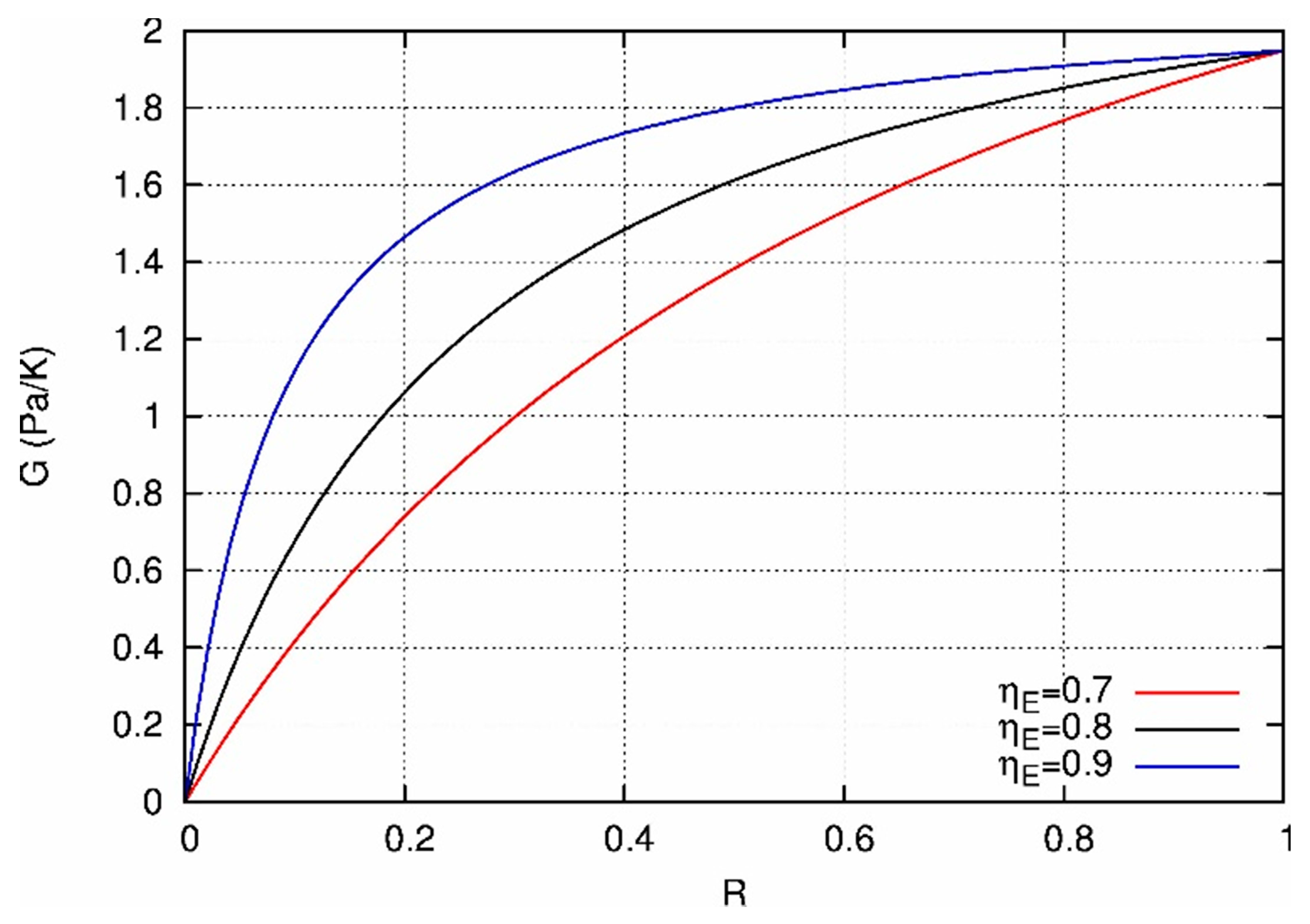
| G | The slope of the mixing line | pa/K |
| Fuel mass flow rate | kg/s | |
| p | Ambient pressure | pa |
| Electric power | W | |
| Q | The lower heating value of fuel | MJ/kg |
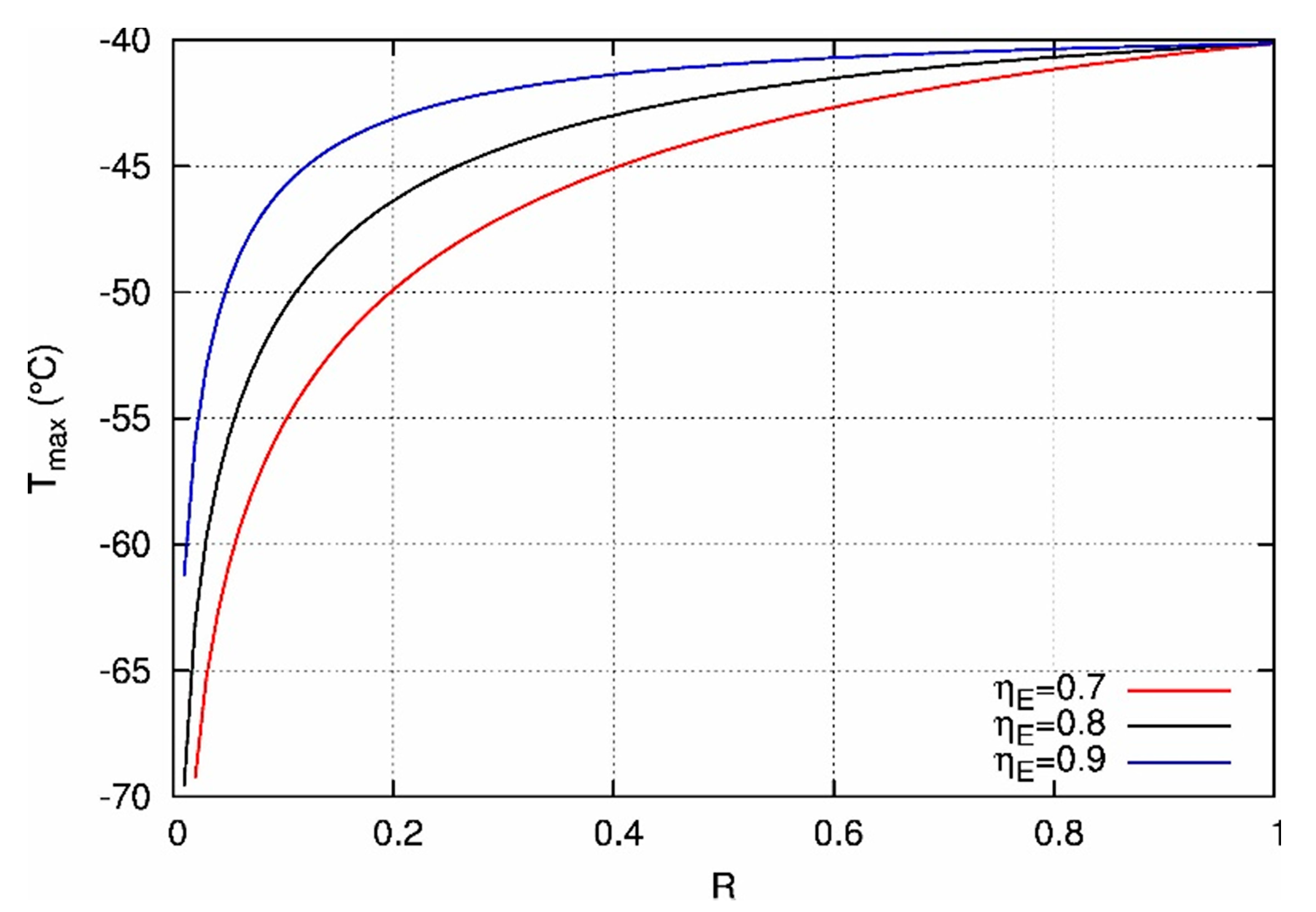
| R | Degrees of hybridization | [−] |
| The maximum temperature at which contrail formation is possible | °C | |
| V | Velocity | m/s |
| ε | The ratio of the molar mass of water vapor and dry air | [−] |
| The overall efficiency of the electric powertrain | [−] | |
| The overall efficiency of the pure kerosene aircraft | [−] |
Appendix A. Derivation of Schmidt–Appleman Criterion for Hybrid-Electric Aircraft
References
- Airbus. Global Market Forecast: Global Networks, Global Citizens 2018–2037; Airbus: Toulouse, France, 2018. [Google Scholar]
- Lee, D.S.; Fahey, D.W.; Forster, P.M.; Newton, P.J.; Wit, R.C.N.; Lim, L.L.; Owen, B.; Sausen, R. Aviation and global climate change in the 21st century. Atmos. Environ. 2009, 43, 3520–3537. [Google Scholar] [CrossRef] [PubMed] [Green Version]
- Grewe, V.; Dahlmann, K.; Flink, J.; Frömming, C.; Ghosh, R.; Gierens, K.; Heller, R.; Hendricks, J.; Jöckel, P.; Kaufmann, S.; et al. Mitigating the Climate Impact from Aviation: Achievements and Results of the DLR WeCare Project. Aerospace 2017, 4, 34. [Google Scholar] [CrossRef]
- Burkhardt, U.; Kärcher, B. Global radiative forcing from contrail cirrus. Nat. Clim. Chang. 2011, 1, 54. [Google Scholar] [CrossRef] [Green Version]
- Søvde, O.A.; Matthes, S.; Skowron, A.; Iachetti, D.; Lim, L.; Owen, B.; Hodnebrog, Ø.; Di Genova, G.; Pitari, G.; Lee, D.S.; et al. Aircraft emission mitigation by changing route altitude: A multi-model estimate of aircraft NOx emission impact on O3 photochemistry. Atmos. Environ. 2014, 95, 468–479. [Google Scholar] [CrossRef]
- Voigt, C.; Schumann, U.; Jessberger, P.; Jurkat, T.; Petzold, A.; Gayet, J.F.; Krämer, M.; Thornberry, T.; Fahey, D.W. Extinction and optical depth of contrails. Geophys. Res. Lett. 2011, 38. [Google Scholar] [CrossRef] [Green Version]
- Schumann, U.; Graf, K. Aviation-induced cirrus and radiation changes at diurnal timescales. J. Geophys. Res. Atmos. 2013, 118, 2404–2421. [Google Scholar] [CrossRef] [Green Version]
- Bock, L.; Burkhardt, U. Reassessing properties and radiative forcing of contrail cirrus using a climate model. J. Geophys. Res. Atmos. 2016, 121, 9717–9736. [Google Scholar] [CrossRef] [Green Version]
- Righi, M.; Hendricks, J.; Sausen, R. The global impact of the transport sectors on atmospheric aerosol: Simulations for year 2000 emissions. Atmos. Chem. Phys. 2013, 13, 9939–9970. [Google Scholar] [CrossRef] [Green Version]
- Schumann, U.; Penner, J.E.; Chen, Y.; Zhou, C.; Graf, K. Dehydration effects from contrails in a coupled contrail–climate model. Atmos. Chem. Phys. 2015, 15, 11179–11199. [Google Scholar] [CrossRef] [Green Version]
- Ciais, P.; Sabine, C.; Bala, G.; Bopp, L.; Brovkin, V.; Canadell, J.; Chhabra, A.; DeFries, R.; Galloway, J.; Heimann, M.; et al. Carbon and Other Biogeochemical Cycles; Cambridge University Press: Cambridge, UK; New York, NY, USA, 2013. [Google Scholar]
- Grewe, V.; Frömming, C.; Matthes, S.; Brinkop, S.; Ponater, M.; Dietmüller, S.; Jöckel, P.; Garny, H.; Tsati, E.; Dahlmann, K. Aircraft routing with minimal climate impact: The REACT4C climate cost function modelling approach (V1. 0). Geosci. Model Dev. 2014, 7, 175–201. [Google Scholar] [CrossRef] [Green Version]
- Matthes, S.; Grewe, V.; Dahlmann, K.; Frömming, C.; Irvine, E.; Lim, L.; Linke, F.; Lührs, B.; Owen, B.; Shine, K.; et al. A Concept for Multi-Criteria Environmental Assessment of Aircraft Trajectories. Aerospace 2017, 4, 42. [Google Scholar] [CrossRef] [Green Version]
- Campbell, S.E.; Bragg, M.B.; Neogi, N.A. Fuel-Optimal Trajectory Generation for Persistent Contrail Mitigation. J. Guid. Control. Dyn. 2013, 36, 1741–1750. [Google Scholar] [CrossRef]
- Zou, B.; Buxi, G.S.; Hansen, M.J.N.; Economics, S. Optimal 4-D Aircraft Trajectories in a Contrail-sensitive Environment. Netw. Spat. Econ. 2016, 16, 415–446. [Google Scholar] [CrossRef]
- Hartjes, S.; Hendriks, T.; Visser, D. Contrail Mitigation Through 3D Aircraft Trajectory Optimization. In Proceedings of the 16th AIAA Aviation Technology, Integration, and Operations Conference, Washington, DC, USA, 13–17 June 2016. [Google Scholar] [CrossRef]
- Yin, F.; Grewe, V.; Frömming, C.; Yamashita, H. Impact on flight trajectory characteristics when avoiding the formation of persistent contrails for transatlantic flights. Transp. Res. Part D Transp. Environ. 2018, 65, 466–484. [Google Scholar] [CrossRef]
- Appleman, H. The formation of exhaust condensation trails by jet aircraft. Bull. Am. Meteorol. Soc. 1953, 34, 14–20. [Google Scholar] [CrossRef] [Green Version]
- Schmidt, E. Die Entstehung von Eisnebel aus den Auspuffgasen von Flugmotoren. Schriften der Deutschen Akademie der Luftfahrtforschung 1941, 5, 1–15. [Google Scholar]
- Faggiano, F.; Vos, R.; Baan, M.; Dijk, R.V. Aerodynamic Design of a Flying V Aircraft. In Proceedings of the 17th AIAA Aviation Technology, Integration, and Operations Conference, Denver, CO, USA, 5–9 June 2017. [Google Scholar] [CrossRef] [Green Version]
- Brand, J.; Sampath, S.; Shum, F.; Bayt, R.L.; Cohen, J. Potential use of hydrogen in air propulsion. In Proceedings of the AIAA/ICAS International Air and Space Symposium and Exposition: The Next 100 Y, Dayton, OH, USA, 14–17 July 2003. [Google Scholar]
- Pohl, H.W.; Malychev, V.V. Hydrogen in future civil aviation. Int. J. Hydrogen Energy 1997, 22, 1061–1069. [Google Scholar] [CrossRef]
- Janic, M. Is liquid hydrogen a solution for mitigating air pollution by airports? Int. J. Hydrogen Energy 2010, 35, 2190–2202. [Google Scholar] [CrossRef]
- Yin, F.; Gangoli Rao, A.; Bhat, A.; Chen, M. Performance assessment of a multi-fuel hybrid engine for future aircraft. Aerosp. Sci. Technol. 2018, 77, 217–227. [Google Scholar] [CrossRef] [Green Version]
- Gladin, J.C.; Perullo, C.; Tai, J.C.; Mavris, D.N. A Parametric Study of Hybrid Electric Gas Turbine Propulsion as a Function of Aircraft Size Class and Technology Level. In Proceedings of the 55th AIAA Aerospace Sciences Meeting, Grapevine, TX, USA, 9–13 January 2017. [Google Scholar] [CrossRef]
- Ang, A.W.X.; Gangoli Rao, A.; Kanakis, T.; Lammen, W. Performance analysis of an electrically assisted propulsion system for a short-range civil aircraft. Proc. Inst. Mech. Eng. Part G J. Aerosp. Eng. 2019, 233, 1490–1502. [Google Scholar] [CrossRef] [Green Version]
- Holsteijn, M.R.V.; Rao, A.G.; Yin, F. Operating characteristics of an electrically assisted turbofan engine. In Proceedings of the AMSE Turbo Expo: Turbomachinery Technical Conference & Exposition, London, UK, 21–25 September 2020. [Google Scholar]
- Sausen, R.; Gierens, K.; Ponater, M.; Schumann, U. A diagnostic study of the global distribution of contrails Part I: Present day climate. Theor. Appl. Climatol. 1998, 61, 127–141. [Google Scholar] [CrossRef] [Green Version]
- Gierens, K.; Kärcher, B.; Mannstein, H.; Mayer, B. Aerodynamic Contrails: Phenomenology and Flow Physics. J. Atmos. Sci. 2009, 66, 217–226. [Google Scholar] [CrossRef]
- Gierens, K.; Dilger, F. A climatology of formation conditions for aerodynamic contrails. Atmos. Chem. Phys. 2013, 13, 10847–10857. [Google Scholar] [CrossRef] [Green Version]
- Jöckel, P.; Kerkweg, A.; Pozzer, A.; Sander, R.; Tost, H.; Riede, H.; Baumgaertner, A.; Gromov, S.; Kern, B. Development cycle 2 of the Modular Earth Submodel System (MESSy2). Geosci. Model Dev. 2010, 3, 717–752. [Google Scholar] [CrossRef] [Green Version]
- Lamarque, J.-F.; Dentener, F.; McConnell, J.; Ro, C.-U.; Shaw, M.; Vet, R.; Bergmann, D.; Cameron-Smith, P.; Dalsoren, S.; Doherty, R.; et al. Multi-model mean nitrogen and sulfur deposition from the Atmospheric Chemistry and Climate Model Intercomparison Project (ACCMIP): Evaluation of historical and projected future changes. Atmos. Chem. Phys. 2013, 13, 7997–8018. [Google Scholar] [CrossRef] [Green Version]
- Jöckel, P.; Tost, H.; Pozzer, A.; Kunze, M.; Kirner, O.; Brenninkmeijer, C.A.M.; Brinkop, S.; Cai, D.S.; Dyroff, C.; Eckstein, J.; et al. Earth System Chemistry integrated Modelling (ESCiMo) with the Modular Earth Submodel System (MESSy) version 2.51. Geosci. Model Dev. 2016, 9. [Google Scholar] [CrossRef] [Green Version]
- Gierens, K.; Lim, L.; Eleftheratos, K. A Review of Various Strategies for Contrail Avoidance. Open Atmos. Sci. J. 2008, 2, 1–7. [Google Scholar] [CrossRef] [Green Version]
- Schumann, U.M. Influence of Propulsion Efficiency on Contrail Formation. Aerosp. Sci. Technol. 2000, 4, 391–401. [Google Scholar] [CrossRef] [Green Version]
- Varyukhin, A.N.; Suntsov, P.S.; Gordin, M.V.; Zakharchenko, V.S.; Rakhmankulov, D.Y. Efficiency Analysis of Hybrid Electric Propulsion System for Commuter Airliners. In Proceedings of the 2019 International Conference on Electrotechnical Complexes and Systems (ICOECS), Ufa, Russia, 21–25 October 2019; pp. 1–3. [Google Scholar] [CrossRef]
- Boies, A.M.; Stettler, M.E.J.; Swanson, J.J.; Johnson, T.J.; Olfert, J.S.; Johnson, M.; Eggersdorfer, M.L.; Rindlisbacher, T.; Wang, J.; Thomson, K.; et al. Particle Emission Characteristics of a Gas Turbine with a Double Annular Combustor. Aerosol Sci. Technol. 2015, 49, 842–855. [Google Scholar] [CrossRef] [Green Version]


| Parameters | Descriptions | Hybrid-Electric Aircraft | Conventional Aircraft | Units | |
|---|---|---|---|---|---|
| Electric power fraction | 40% | 80% | 0 | [−] | |
| EIH2O | Water emission index | 1.25 | kg/kg(fuel) | ||
| η | Overall efficiency | 0.8 | 0.4 | [−] | |
| Q | The lower heating value of the fuel | 43.2 | MJ/kg | ||
| G | Slope at 11 km altitude | 1.6 | 1.1 | 1.8 | Pa/K |
© 2020 by the authors. Licensee MDPI, Basel, Switzerland. This article is an open access article distributed under the terms and conditions of the Creative Commons Attribution (CC BY) license (http://creativecommons.org/licenses/by/4.0/).
Share and Cite
Yin, F.; Grewe, V.; Gierens, K. Impact of Hybrid-Electric Aircraft on Contrail Coverage. Aerospace 2020, 7, 147. https://doi.org/10.3390/aerospace7100147
Yin F, Grewe V, Gierens K. Impact of Hybrid-Electric Aircraft on Contrail Coverage. Aerospace. 2020; 7(10):147. https://doi.org/10.3390/aerospace7100147
Chicago/Turabian StyleYin, Feijia, Volker Grewe, and Klaus Gierens. 2020. "Impact of Hybrid-Electric Aircraft on Contrail Coverage" Aerospace 7, no. 10: 147. https://doi.org/10.3390/aerospace7100147
APA StyleYin, F., Grewe, V., & Gierens, K. (2020). Impact of Hybrid-Electric Aircraft on Contrail Coverage. Aerospace, 7(10), 147. https://doi.org/10.3390/aerospace7100147