Trajectory Planning in Time-Varying Adverse Weather for Fixed-Wing Aircraft Using Robust Model Predictive Control


Department of Mechanical, Automotive and Aeronautical Engineering, University of Applied Sciences Munich, 80335 Munich, Germany
Aerospace 2019, 6(6), 68; https://doi.org/10.3390/aerospace6060068
Submission received: 9 April 2019
/
Revised: 17 May 2019
/
Accepted: 30 May 2019
/
Published: 5 June 2019
(This article belongs to the Special Issue Aircraft Trajectory Design and Optimization)
Abstract
:The avoidance of adverse weather is an inevitable safety-relevant task in aviation. Automated avoidance can help to improve safety and reduce costs in manned and unmanned aviation. For this purpose, a straightforward trajectory planner for a single-source-single-target problem amidst moving obstacles is presented. The functional principle is explained and tested in several scenarios with time-varying polygonal obstacles based on thunderstorm nowcast. It is furthermore applicable to all kinds of nonholonomic planning problems amidst nonlinear moving obstacles, whose motion cannot be described analytically. The presented resolution-complete combinatorial planner uses deterministic state sampling to continuously provide globally near-time-optimal trajectories for the expected case. Inherent uncertainty in the prediction of dynamic environments is implicitly taken into account by a closed feedback loop of a model predictive controller and explicitly by bounded margins. Obstacles are anticipatory avoided while flying inside a mission area. The computed trajectories are time-monotone and meet the nonholonomic turning-flight constraint of fixed-wing aircraft and therefore do not require postprocessing. Furthermore, the planner is capable of considering a time-varying goal and automatically plan holding patterns.
1. Introduction
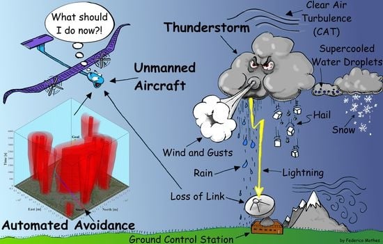
Weather avoidance is an ever-present and safety-relevant task in manned and unmanned aviation. Approximately every fifth accident in commercial aviation and every fourth in general aviation is related to adverse weather [1,2]. Especially thunderstorms and their surroundings are dangerous, as turbulence, gusts, wind shear, lightning, hail and icing may occur. According to the Federal Aviation Administration (FAA), the philosophy of avoidance is an integral part of flight planning [3]. This is especially true for light unmanned fixed-wing aircraft, for example high altitude pseudo-satellites [4]. Their relatively low weight and performance increase the vulnerability to adverse weather [5].
Thus far, the operation of these aircraft requires a considerable amount of manual effort in mission planning and execution. Many of the incurring tasks are related to tactical flight planning based on external meteorological information, as some aircraft are not equipped with an onboard weather radar. For this purpose, pilots and meteorologists have to consider a great amount of information all at once, i.e., actual and future aircraft states, airspace restrictions and time-variant forecasts under consideration of their uncertainty. However, memory capacity of humans is usually limited to 7 ± 2 chunks of information [6], which is clearly insufficient to make optimal use of the available information. In complex scenarios with moving obstacles, this shortcoming can be partially compensated by applying quasi-static planning: Moving obstacles are avoided by an imaginary static radius of action plus an additional margin to account for uncertainty. This method works well when the aircraft is fast in relation to the obstacles. However, convective weather has a high rate of change and quasi-static avoidance is prone to cause reactive flight guidance. Reactive trajectories are suboptimal in terms of safety, mission accomplishment and energy consumption. For unmanned aircraft, a loss of link in both line of sight and beyond line of sight communication is a potential incident. The ability to continue flight in these situations, at least for a short period of time, enhances their level of autonomy and safety [7]. The intrinsic complexity of anticipatory trajectory planning in uncertain dynamic environments calls for an automated solution. The consideration of kinematic and dynamic constraints further raises the complexity of this task [8,9].
The configuration q of an aircraft is a combination of its degrees of freedom. The configuration space C with can be used for path planning in static environments. When dealing with moving obstacles, reactive planners use the static C-space to perform replanning whenever the environment changes [10,11]. However, for anticipatory trajectory planning in the presence of moving obstacles, time has to be added to the C-space. Therefore, even two-dimensional motion planning problems are difficult to solve as the dimensions are raised from two to three [12]. A trajectory in this case is a path that is parameterized by monotonically increasing time and is compliant with kinematic and differential constraints of the aircraft. Erdmann and Lozano-Perez [13] introduced the concept of configuration × time-space, which is also called state space (X-space). Time-dependent configurations are called states with [14]. Provided that a knowledge or estimate of the future obstacles exists, a sequence of states leading from start to goal state has to be determined. For this task, different motion planning methods exist.
An example for a control theory approach, regarding motion planning amid time-varying thunderstorms, is found in [15]. A finite horizon reach-avoid problem formulation [16] is used to maximize the probability of reaching a given point, while avoiding stochastic obstacles, under the consideration of uncertainties. Due to the curse of dimensionality [17], this kind of approach is unsuitable for fast computation of problems with high degrees of freedom.
Classic robotic approaches for motion planning amid moving obstacles include sampling-based and combinatorial motion planning. Rapidly-exploring random trees (RRTs) belong to the family of sampling-based algorithms. They are extremely popular due to their ability to quickly find feasible trajectories in X-space, for problems with high degrees of freedom and complicated constraints [18,19]. Examples for kinodynamic planning amidst moving obstacles can be found in [20,21,22]. However, narrow passages can pose a problem, as the likelihood for a sample being in free space decreases. Furthermore, trajectories tend to be jerky and therefore require postprocessing, e.g., by B-splines, Bézier curves or clothoids [23]. As random samples are used, the algorithm is probabilistically complete. This means that, if a trajectory exists and the number of samples approaches infinity, the probability to find the trajectory converges to one.
In [8], a combinatorial method for kinodynamic planning is presented. The upper bound for the complexity of exact motion planning in a three-dimensional dynamic environment is given by a general algorithm with a time complexity that is double exponential in the dimension of search space [24]. Canny [25] introduced an algorithm where time complexity is only exponential in its dimension. A combinatorial motion planner searches a discrete topology of free space, e.g., a visibility graph, Voronoi diagram or an exact or approximate cell decomposition. The explicit representation of the search space limits the application of combinatorial methods to problems with low degrees of freedom, i.e., the number of parameters necessary to specify q [14]. Nonetheless, combinatorial planning offers desirable properties such as optimality, completeness and repeatable results that can be important for certification.
In this article, a combinatorial motion planner, called MPTP (see Section 2.1), is described that computes collision-free, near-time-optimal and time-monotone trajectories from to similar to [26,27]. Global optimization is performed using an A*-search algorithm [28]. Motion planning in the real-world is generally subject to uncertainty in environment and state predictability [14]. In the presented setup, the planner solely relies on external environment prediction, in this case thunderstorm nowcasts. The immanent uncertainty in the environmental prediction is taken into account explicitly by bounded margins and implicitly by the closed loop of a model predictive controller (MPC). While planning takes place, information outdates in dynamic environments. This imposes a real-time decision constraint and limits the allotted time for trajectory planning [29]. For fast convergence, the X-space is iteratively built and its growth is restricted by a suitable heuristic. Furthermore, velocity and angle of climb are assumed to be at least piecewise constant. The planner uses a low-fidelity representation of aircraft dynamics with motion primitives. This ensures that the computed trajectories are compliant with the aircraft’s flight envelope and resulting tracking errors are small [30].
The planner can be used as initial guess generator for gradient-based trajectory optimization in dynamic environments similar to Dubins path does in static environments to find an optimal control sequence in the homotopy class of the initial guess with a high-fidelity aircraft model [14,31].
The rest of this article is organized as follows. In Section 2, the functional principle and technical details of the presented trajectory planner for dynamic environments are described. Section 3 presents simulation results of the key capabilities, followed by the discussion (Section 4) and conclusions (Section 5).
2. Methodology
2.1. Model Predictive Trajectory Planning
The focus of this article lies on the introduction of an anticipatory trajectory planning algorithm for automated aircraft guidance through time-varying adverse weather, for example thunderstorms. Planning is performed by a reactive guidance loop, which resembles a MPC setup, due to the feedback of state and weather information. It is hence termed model predictive trajectory planner (MPTP) and provides resolution-complete and globally near-optimal trajectories for the expected case. Periodically, a new trajectory is computed, which attempts to always avoid adverse weather based on the latest nowcast. A fixed-wing aircraft has a nonholonomic turning-flight constraint and flies with finite velocity. The kinematic constraints are to avoid moving polygonal obstacles while staying within a defined mission area. In aviation, safety has the highest priority. Therefore, an optimal trajectory is defined here as the one that takes the shortest time to get to the goal while staying clear of potentially dangerous areas. As it is difficult to determine the appropriate altitude for vertical avoidance of thunderstorms (visible top is not necessarily equal to the radar top) and turbulence is frequently encountered above storm clouds, the focus lies on lateral avoidance [32].
Provided an appropriate flight controller (FC) is equipped and considering the guidance constraints in MPTP (see Section 2.3.4), it can be expected that an aircraft is able to fly the commanded trajectories. In this article, the assumption is made that commanded states are reached in due time, so that a next initial state (see Section 2.2.2) is part of the previously computed trajectory. Hence, the FC and aircraft blocks are not modeled. While this setup is not eligible to prove the feasibility of the proposed guidance strategy, it is appropriate to explain the presented trajectory planning algorithm (see Section 2.2 and Section 2.3), demonstrate continuous avoidance trajectories on the basis of real thunderstorm forecasts, and compare different computation methods (see Section 3). However, in [4], the feasibility of the proposed guidance strategy is demonstrated with the setup depicted in Figure 1. The simulations are done using a six degree of freedom aircraft model, flight controller and historical wind data.
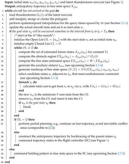
The inputs for the MPTP are the nowcast and a mission planner which specifies the reference, i.e., the goal state. The planning and control horizon of the MPTP are equal to the nowcast horizon of one hour. The control output is a sequence of states, which is sent to the FC with a sampling time that is equal to the nowcast update interval of s.
The MPTP, which plans with a low-fidelity aircraft model at a low update rate, and FC, which operates on the actual aircraft at a high update rate, are decoupled as in [33,34]. The FC is the reactive component which compensates disturbances and uncertainties and controls the aircraft in order to reach the commanded states in due time.
Thunderstorms have a short life span and their development is very difficult to predict. The uncertainty in the nowcast is implicitly considered by updates (predicted disturbances in Figure 1) and control errors by the closed loop of the MPTP (initial state in Figure 1). The recurrent correction of errors due to unpredicted disturbances yields robustness [33]. Periodical replanning of anticipatory trajectories from the actual state to the goal is done in each iteration based on the latest nowcast. Predicted thunderstorm cells are represented as spatial and temporal discrete polygonal obstacles with nonlinear motion.
The MPTP consists of a prediction and optimization module. To find a feasible trajectory to the goal, the MPTP iterates between those two (Figure 1): The prediction interprets nowcast data and estimates future conflicts between aircraft and thunderstorms (see Section 2.2) to generate a representation of free state space [14]. For the optimization, a combinatorial motion planning method with bounded uncertainty is applied (see Section 2.3). The discrete time increment for prediction and optimization has to be a factor of the nowcast update interval with .
2.2. Prediction–Conflict Estimation
The prediction module of the aforementioned MPTP consists of three models. The first model predicts the obstacles, i.e., the expected future thunderstorms. For this purpose, the nowcast is interpreted regarding the relative hazard for a specific aircraft taking into account the immanent uncertainty. The second prediction model computes future aircraft state samples. A third model superimposes the first two models to estimate future conflicts. As the term conflict seems more appropriate than collision in the context of weather avoidance, it is used exclusively throughout the rest of the article.
2.2.1. Expected Future Obstacle Locations
Thunderstorms and their surroundings are extremely dangerous for all kind of aircraft. The expectation of their future location is based on historical thunderstorm nowcast issued by the algorithm Radar Tracking and Monitoring (Rad-TRAM) [35]. Historical data are provided in Extensible Markup Language format (XML) by the German Aerospace Center DLR. A XML-file contains nowcasts as well as corresponding measurements. Thunderstorms are represented as polygons, which ensures small file size and allows fast processing [36]. The nowcast has a temporal horizon of one hour and is updated every five minutes. Each nowcast consists of 13 sets containing the coordinates of storm cells and additional information, e.g., center of gravity, moving direction and moving speed. The first set contains the measured thunderstorm situation, while the others are predictions with an interval of 5 min. Information about the wind field on standard flight levels is based on COSMO-DE model [37] data and supplied in General Regularly-distributed Information in Binary form (GRIB). The forecast horizon is 21 h and the update interval is one hour [38].
In aviation a minimum lateral clearance to thunderstorms (especially cumulonimbus clouds) is recommended [32,39]. To compute safe trajectories, the weather data have to be interpreted with respect to the limitations of an aircraft. For this purpose, storm cells are expanded by appropriate margins. Two kinds of margin are applied to nowcasted cells, which are described in the following. Their purpose is to account for different kinds of uncertainty regarding the weather information.
Due to initial condition uncertainties and model errors, forecasts are never accurate [40]. Especially convective weather has a high rate of change and is difficult to predict. The forecast error generally increases with advancing time. This fact can be explicitly modeled applying bounded uncertainty, as proposed by Sauer et al. [41]. Thunderstorm cells are enlarged by nonuniform probabilistic margins. Their size is a function of a selected probability P that a cell will be included by its corresponding margin at a given time in the nowcast horizon . This is a safe procedure especially when assuming high values for P. As the presented MPTP computes trajectories based on the expected case, an overestimation of uncertainty leads to excessive coverage of free airspace. This directly affects the optimality of trajectories and sometimes even prevents that a solution can be found [14]. The ability to automatically plan holding patterns (Section 2.3.5) can solve some of the cases in which the goal is covered or the access to the goal is blocked. The applied strategy is to compute trajectories in parallel using different probabilities P and then choosing the feasible solution with the highest P or rather largest margins.
In contrast to the aforementioned margins, the safety margins account for the uncertainty regarding the presence of thunderstorm accompanying phenomena, e.g., strong winds, wind shear, turbulence (clear air turbulence over and downwind of cumulonimbus clouds), lightning, icing and hail. These phenomena are hardly predictable and often detected as late as when being in situ. This is why FAA requires minimum distances to thunderstorms [39,42]. These safety margins are independent from the nowcast time. Their size partly depends on the structural limits of an aircraft and furthermore on appearance, size and moving speed of a cell as these parameters allow conclusions on the potential danger. In most cases, it is safer to avoid thunderstorms on the upwind side as turbulence and hail is frequently encountered downwind [32]. By enlarging cells in these areas, the planner is tempted to shift the trajectory. By applying the aforementioned margins to concave thunderstorm polygons, they are transformed into convex polygons. This is reasonable as concave radar signatures are associated with strong turbulence and hail [32]. The superposition of probabilistic and safety margins can be seen in the Figure in Section 3.1 as light red areas around the predicted dark red thunderstorms.
High thunderstorm density and close neighboring cells indicate potentially weather active areas. They are dangerous because the uncertainty in the nowcast is locally high and sudden changes may happen. The FAA advises to circumnavigate weather active areas with a thunderstorm coverage of 6/10 or higher [39]. An intuitive interpretation is necessary to identify weather active areas, as planning trajectories through them can cause substantial short-term changes with respect to the initial route. Discrete margins sometimes leave narrow passages between thunderstorms of which the MPTP makes use of when searching for a trajectory. To avoid this, Density Based Spatial Clustering for Applications with Noise (DBSCAN) is applied with the radius for neighborhood determination () set to a selected minimum corridor width [43]. In many cases, clustering of thunderstorms result in concave polygons. These are not converted to convex polygons, as otherwise excessive coverage of free space is the consequence [44].
Finally, a processed nowcast results in thirteen discrete sets of buffered thunderstorms ( min, min, …, min). However, the MPTP requires discrete information concerning the obstacles for the intermediate query times spaced by . This is achieved by applying a linear spatiotemporal interpolation. For instance, if s, four interpolated polygonal shapes for each known shape (thunderstorm) are computed for s, s, s and s. An example for this procedure can be found in [44].
2.2.2. Estimated Future Aircraft States
Future states of the aircraft are estimated in the Earth fixed frame with the basic idea of a wavefront propagating with constant true airspeed . The radial distance between isochronous state sets is in the absence of wind. For the estimation of future states, two cases have to be distinguished, namely wind speed or . In the real world, wind speed is rarely zero. What matters is if the aircraft or more specifically the FC can compensate the wind.
If wind can be compensated, future state primitives for up to one hour of flight can be preprocessed for different ground speeds with for . For this purpose, a 3DOF simulation model of the aircraft is used. The formulas of the aircraft’s motion are
with being the bank angle. The derivatives of the velocity V, course or track angle and the angle of climb are given, respectively, by
Additionally, the horizontal and vertical load factors and are needed with T being the thrust, m the mass, g the Earth’s gravitation, D the drag and L the lift.
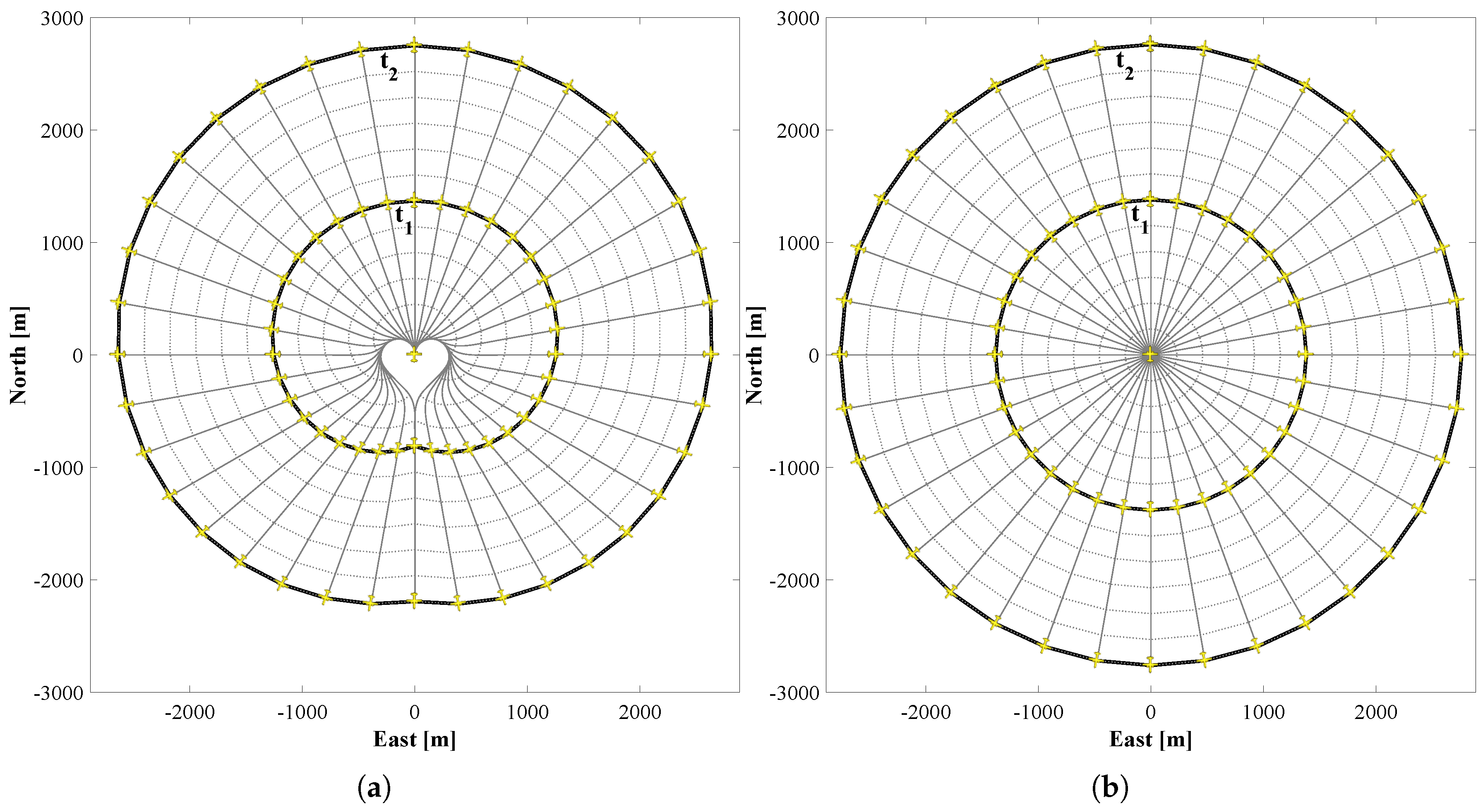
A controller keeps the aircraft model on commanded courses between . The controller consists of three laws for altitude, speed and azimuth control. The connection between contemporary state samples results in isochronous curves (black lines in Figure 2a). The heart shape in Figure 2a results from turning-flight when changing the initial course from north by .
The estimated set of future aircraft state samples are computed in a Cartesian coordinate system heading north. To obtain the set of future estimated aircraft states from an arbitrary initial state , the are rotated around the z-axis according to the initial course and translated in all three spatial dimensions by a homogeneous transformation matrix with , written-out:
If the wind field is considered, future states cannot be preprocessed as the resulting depends on the position and course of the aircraft. To compute a trajectory, future states have to be computed several times (see Section 2.3). The considerable computation time when using a flight simulation makes this method unsuitable for online application.
If the curve, due to the initial turning-flight when changing the course, is ignored, future aircraft states can be approximated with a marching wave expanding from the initial position (see Figure 2b). The easiest way is to set up linearly spaced matrices for each spatial dimension. The first dimension of each matrix indicates the time t and the second dimension the course . Alternatively, the first-order nonlinear partial differential Eikonal equation in the form can be applied with T being the arrival times of the expanding wave and F being a scalar speed function. If wind is not considered, it can be efficiently solved using the isotropic fast marching method (FMM) in , with n being the number of grid points [45,46]. This finite-difference method is suitable for online application. Using the multistencils second order fast marching method (MSFMM) improves the accuracy considerably [47]. However, for slow aircraft, wind has a significant impact on trajectory planning, as it cannot always be completely compensated. Under the influence of wind, constant results in a spatially inhomogeneous profile. If the wind is considered for planning, a noniterative ordered upwind method (OUM) can be applied for a fast approximate estimation of future aircraft states [48,49].
2.2.3. Estimated Future Conflict Areas
Obstacle regions with invalid are called [14]. Originating from an initial state ∈X, deterministic samples of estimated future aircraft states are used to perform a conflict check with contemporaneous obstacles to create an explicit representation of the estimated obstacle region . This is done by superposition of the aforementioned prediction models for expected future obstacle location and estimated future aircraft states. The set of estimated conflicts from an initial state is defined as the union of the set of future aircraft states and set O of time-varying obstacles with arbitrary shape that depends on time t. Future states on and inside of time-varying obstacles are enclosed by concave polygons that are called estimated conflict areas (ECA) with . The estimated obstacle region is the union set . The mission area, in which the aircraft is allowed to fly, is called the workspace . The free estimated state-space is the difference .
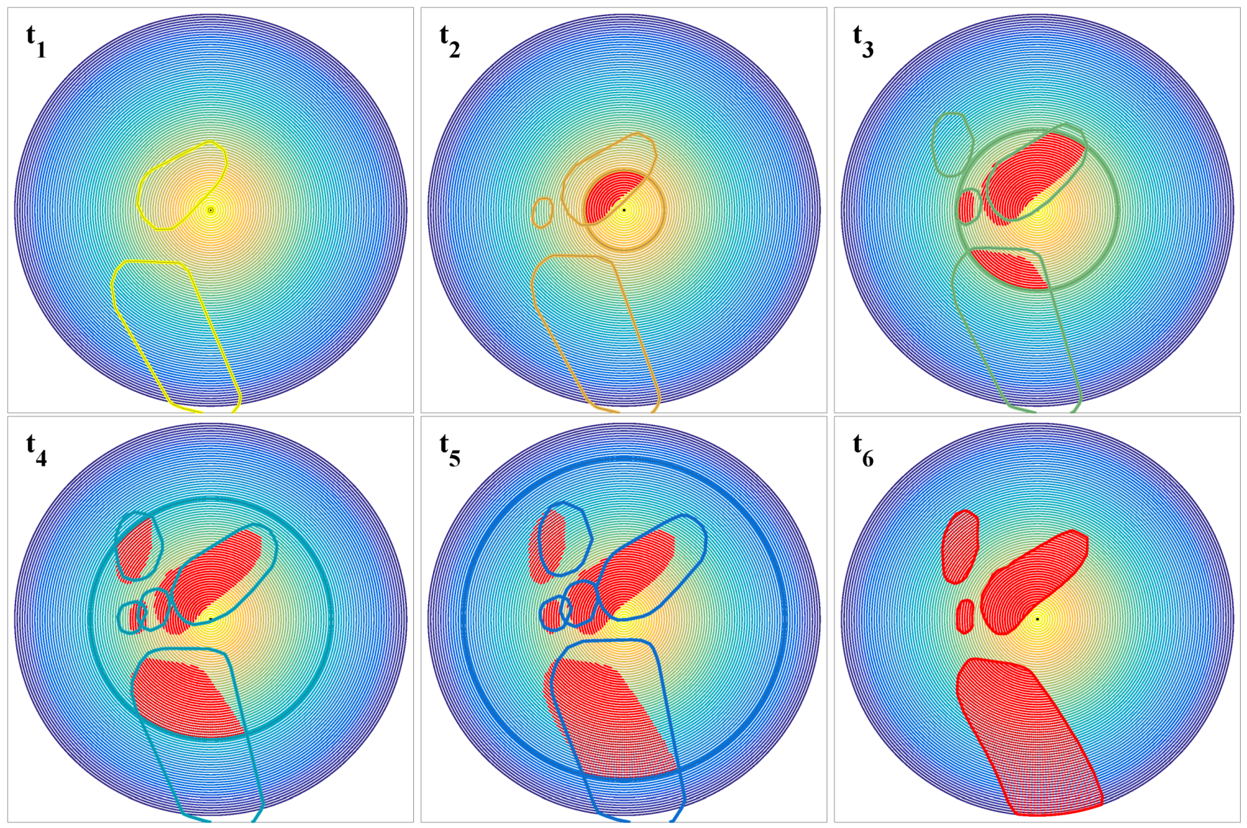
Figure 3 shows an example for the evolution of under the assumption of constant . The isochronous circles can be interpreted as level sets of a cone that opens perpendicular in the third dimension that represents the time with the initial state in the center. Contemporary conflicts are depicted in red.
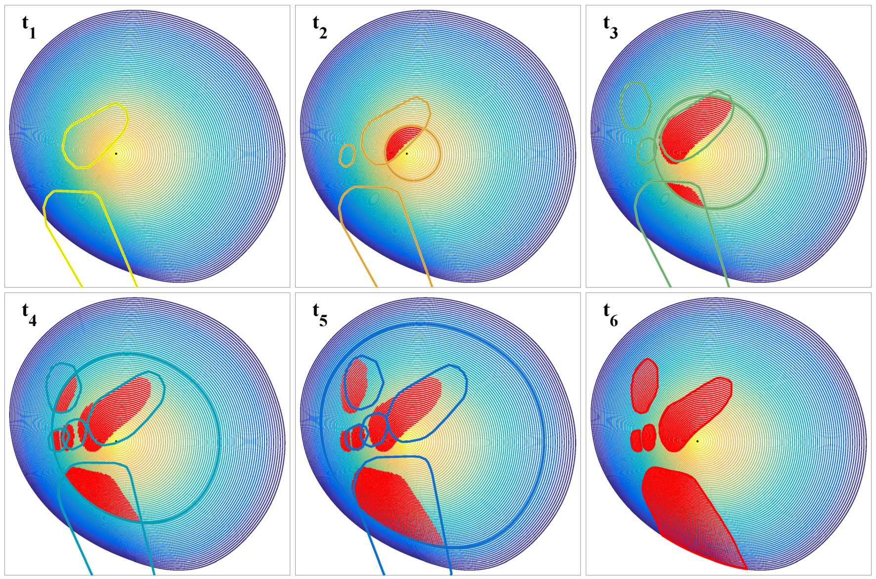
If the wind forecast (Section 2.2.1) is considered the isochronous progress is not circular anymore such as in Figure 4. The shape of the obstacle region is clearly different than in Figure 3.
The presented method can also be used to determine in non-level flight (Figure 5). For this purpose, three-dimensional obstacles are generated by extrusion of different 2D thunderstorm data, i.e., ground and satellite based nowcast. Sufficiently large safety margins are added in all spatial directions. Where estimated future aircraft states are in conflict with an obstacle, an estimated conflict surface () is generated. For constant angle of climb , an approximate avoidance trajectory around moving three-dimensional obstacles can be computed for non-level flight, using the methods in Section 2.3.
2.3. Optimization–Trajectory Computation
This section explains the necessary steps to find a time-monotone trajectory through predicted thunderstorms under the consideration of the nonholonomic turning-flight constraint.
2.3.1. Graph of Free Estimated State Space
A visibility graph is used to create a roadmap of (Section 2.2.3) from an initial state . It contains vertices and edges which are undirected and weighted. Rohnert [50] introduced a method to compute a reduced for convex polygons containing exclusively tangent edges between a point and a polygon and bitangent edges between polygons. LaValle [14] described a robust method to determine bitangent edges without trigonometric functions by using cross products. After excluding all edges that are not tangent or bitangent, the remaining edges are checked for intersections. The vectorized Matlab code works for convex and nonconvex s and optionally generates a partial or complete . A partial visibility graph only connects to vertices that are adjacent by a tangential edge. A complete visibility graph contains all visible edges in . Figure 6 shows a comparison between three different s, inside a mission area (black square) and around obstacles (four red icosagons). The large difference in visible edges (green lines) is the reason only Method b and c are considered for trajectory planning.
The time complexity of the can be expressed by the number of vertices . A reduction of in therefore improves the runtime of the . The time complexity of a graph-search algorithm (see next section) is often described by the number of vertices and edges of the searched graph, e.g., for Dijkstra’s algorithm. A reduction in also reduces and thus speeds up the search. To reduce in , the Douglas–Peucker algorithm can be applied [51]. Through an appropriate selection of the tolerance band , a reduction can be done under preservation of shape, e.g., by an error bound termination condition [52]. Predicted thunderstorms are enlarged by probabilistic margins to model the considerable amount of uncertainty in the nowcast (see Section 2.2.1). Hence, is generated upon a guess of the future and does not represent an absolutely exact geometry. Therefore, small geometric inaccuracies due to line smoothing are acceptable.
2.3.2. Informed Search in a Dynamic Environment
To find anticipatory time-optimal trajectories, A*-search is applied [28]. It is suitable for single-source-single-target problems and has many advantageous properties, namely being a complete, optimal and easy to implement algorithm.
Depending on the applied heuristic (see next section), a partial or complete of is generated. This process is repeated until is equal to the goal state or no solution exists. In the following, the nodes of the are referred to as states. In contrast to the Dijkstra’s algorithm, A* does not just compute the G-cost, which in this case is the time to get from the start state to a candidate state . Instead, it uses an additional heuristic to estimate the H-cost, which is the time to get from a to . The total estimated F-cost is the time it takes to get from to via and is calculated by .
A complete roadmap to the goal in X-space does not exist a priori. Instead, it is iteratively generated by exploring with . The A*-search grows trajectories, which are all rooted in the start state . During every loop of A*, the F-cost for each is computed. The most promising , which has the minimum estimated F-cost, is explored in the next iteration. The bookkeeping is done in the Open List (). For fast computation, the is a priority queue implemented as binary heap that contains all sorted in ascending F-cost order as well as their parent states .
At the beginning of the algorithm, the only state in the is , which automatically has the lowest estimated F-cost. The is computed from . Next, a generates a roadmap of the static . Subsequently, the adjacent states of are inserted into as . Then, is popped from the priority queue and inserted into the so-called Closed List (), which stores already explored states. This process repeats until the is empty, in which case the algorithm reports that no trajectory to the goal exists and performs partial planning, or the goal is inserted into the , in which case the trajectory is constructed by backtracing the corresponding parent states and is then commanded to the FC.
The following pseudocode (Algorithm 1) illustrates the functionality of the MPTP including the A*-search.
| Algorithm 1: MPTP |
 |
In the pseudocode above, the typical relaxation of the A*-search is missing (inside the while loop). In a static environment, A*-algorithm checks if new candidate nodes are already in the or . If their G-cost is lower, the existing entry is updated by replacing the G-cost and parent node. However, in the presented case, the obstacles move. Each is tangential to the s whose form is uniquely valid from the perspective of their . Therefore, even if a has the same q as an explored state and a lower time t from to (which is the G-cost), it cannot replace the state in the or . As each is adjacent to its by a straight line. the final trajectory is guaranteed to be optimal.
2.3.3. Heuristics for the Informed Search
In this section, three different heuristics are described. The quality of the heuristic is essential for the convergence of the A*-search and the optimality of the computed trajectories. For trajectory planning, the H-cost is the estimated time it takes to get from a candidate to the goal state . If this cost is underestimated, the solution is optimal but unnecessary search is done. A heuristic is admissible if it never overestimates costs as this can lead to suboptimal results.
The first and most ineffective heuristic is to set H to a constant value, e.g., equal to zero. Then, A*-search basically becomes Dijkstra’s algorithm and the search expands as a wavefront in all directions.
The Euclidean distance heuristic (EDH) estimates the H-costs, to get from each to , by the beeline distance. It is an admissible and effective heuristic [14]. When Dijkstra or A* with EDH is applied, only a partial with the first order adjacent states has to be computed. This saves computation time in comparison to the generation of a complete . However, EDH ignores obstacles as it only evaluates the beeline to the goal.
Finally, a new shortest static path heuristic (SSPH) is introduced in this article. A complete of every is searched by a nested A*-search. This inner A* for his part applies the EDH to determine the H-cost for every new by computing its shortest path to (which can be converted to time as is constant) in the static . Alternatively, the Fast Marching Method can be applied (see Section 2.2.2). In this case, no is needed, which is especially interesting when searching three-dimensional space. Although SSPH is computationally more intensive than EDH, the explicit consideration of obstacles speeds up the search (see Section 3). However, SSPH can overestimate the H-cost as it is computed in the , which is why optimality of trajectories cannot be guaranteed. Hence, SSPH is a non-admissible heuristic. In practice, Dijkstra, EDH and SSPH produce identical or similar trajectories (see Section 3).
2.3.4. Modeling Nonholonomic Turning-Flight
A fixed-wing aircraft has velocity constraints in the y- and z-direction of its body-fixed frame of reference and cannot fly directly sideways or upwards. While the number of velocities of the aircraft is reduced, there are no restrictions in its configurations as they can be reached performing a series of maneuvers. Therefore, a fixed-wing aircraft is a nonholonomic system [53].
If the future state primitives from Section 2.2.2 are used, the nonholonomic turning-flight constraint is considered innately. For the methods that approximate future states, the nonholonomic constraint has to be explicitly modeled. As the combinatorial planning approach does not model the nonholonomic turning-flight by default, an auxiliary method is required. Additional states, which in the following are referred to as auxiliary states , are generated to obtain discrete curvature-constrained trajectories, which can be interpreted as a discrete version of Dubins path [54]. An can be generated for one turning-sense (unidirectional turning-flight) or both turning-senses (bidirectional turning-flight). A maximum course angle change from is introduced. Adjacent future states to that require are disconnected from in the . The value for cannot be chosen freely, as it has to be ensured that the aircraft is able to reach commanded states in due time.
A straightforward method for the computation of auxiliary states is introduced in the following. Starting from , the initial can be changed by . An is then located on the new course at the leg distance of and can be performed as fly-by or fly-over state. To ensure that a commanded state can be reached in due time, two conditions have to be met. First, the leg distance between the adjacent states has to be greater or equal than the minimum stabilization distance [55]. The MSD is the minimum distance that it takes for the aircraft to fly on the new course. Second, to reach the next commanded state (waypoint at a certain time) in due time, the aircraft has to fly with a corrected mean velocity . Generally, the distance covered by the aircraft (ACD) differs from the . However, the aircraft has to arrive at the next state in . In the case of a fly-by state and , the is . For a fly-over state and , the is . The has to be greater than the stall speed and less or equal to maximum velocity , to ensure feasibility of a trajectory.
In the following, a simple procedure to quickly assess the flyability of states, i.e., admissible combination of selected planning velocity , and , is presented. With the setups in Figure 7, a normalized minimum stabilization distance and velocity correction are determined as a function of (see Table 1 and Table 2), by setting the minimum turning radius to (unit turning-circle). To determine the smallest possible for fly-over states, for both the roll-in and roll-out radius the same radius is applied (see Figure 7b). Generally, roll-in and roll-out radius are different, leading to a smooth trajectory but longer .
The values for the (Table 1 and Table 2) are computed by the aforementioned approximation. Therefore, the establishment of the bank angle and the acceleration, for the correction of the distance per error, are neglected. To account for these factors, a distance of can be added to the , for example with being 10 s for a fly-over state [55].
As the time increment is a fixed value, the relative error between the normalized distance covered by the aircraft () and the normalized minimum stabilization distance () is used to calculate a velocity correction factor. Due to the turn anticipation when performing a fly-by state, the planned distance is twice the (see Figure 7) and the velocity correction factor is computed by
The formula for a fly-over state is
The corrected mean velocity is then computed by
With the value for and , the corresponding minimum turning radius can be computed
By multiplying with the minimum turn-radius , the actual minimum stabilization distance is calculated. Table 3 shows exemplary values for different .
In order for a planned trajectory to be flyable, the minimum time increment is determined by
Notice that the values for the velocity correction in Table 1 and Table 2 only apply for the special case, in which the leg distance is equal to the . Else the corrected mean velocity is less, as the relative error between and is correspondingly smaller. This also implies that is smaller. Therefore, if , an iterative calculation is applied, to solve for the necessary . For fly-over states, this is described by
For the example in Section 3.3, the leg distance is m. In the case of , and , the corresponding value from Table 2 is . Applying the aforementioned formula with a convergence criterion of , the new value is . Therefore, the corrected mean velocity is m/s instead of m/s.
For values of , fly-by states generally result in much shorter and a less critical reduction of the velocity instead, compared to fly-over states. However, even if all states are fly-over, the simulations in Section 3 satisfy the criteria for flyability, i.e., and .
To increase the robustness of the MPTP, the maximum course change can be defined as soft constraint. A is only valid if it is neither in nor on . If no exists, can be increased stepwise, until a exists and is valid, i.e. the actual . If possible, should be kept small, as this generally results in smoother and more optimal trajectories.
2.3.5. Automatic Planning of Holding Patterns
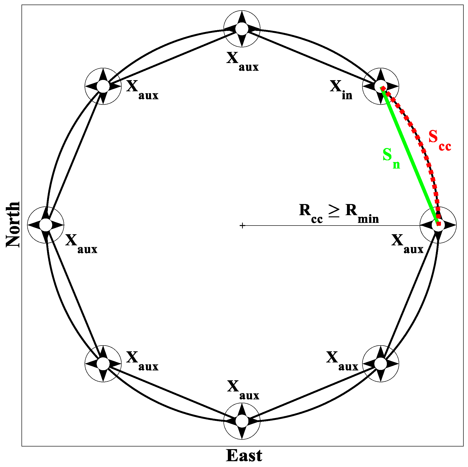
According to the NATO Standardization Agreement No. 4586, the circle is an authorized holding maneuver for unmanned aircraft. Radius, turning-sense and duration of the hold are unrestricted [56]. Before a trajectory is planned, the algorithm determines if the goal will be covered by obstacles in the period from to . If the goal is permanently covered during the period of the actual nowcast, it is declared as not flyable and the aircraft performs a hold in until the next nowcast is issued. It is possible to specify holding locations in advance which the planner can use when they are in . If the goal is only temporarily covered, a holding pattern is performed until the goal is in . Therefore, a unidirectional turning constraint is applied, for example only turn right (UPS-method). This prevents the MPTP to plan meandering trajectories, however they may no longer be near-optimal.It is also important to notice that resulting trajectories can be considerably different, depending on the selected sense of rotation.
The , which are always added to model the nonholonomic turning-flight constraint, naturally result in circular holding patterns in , if the goal is covered. The ability to plan holding patterns therefore exists innately, which is very practical and keeps the algorithm simple.
For example, by setting , a circular holding pattern is described by the , as inscribed regular n-gon with (see Figure 8 and Section 3.3). The distance on a straight segment of an n-gon is given by . For fly-over states, the radius of the corresponding circumcircle, on whose orbit the aircraft flies, is
The distance on the corresponding circumcircle segment is
As , the velocity has to be corrected, in order for the aircraft to arrive at a state in due time. The correction factor is calculated by the relative error of the distances to , as is a fixed value
The mean corrected velocity is calculated by
To ensure the feasibility of a planned trajectory, it is important that and is . In the upcoming example in Section 3.3, the velocity for planning is m/s. Therefore, the corrected velocity is m/s m/s. The required bank angle for the coordinated turn is
This leaves reserves regarding the turning-flight performance. In theory, the flight controller is able to put the presented guidance strategy into practice, arriving at the commanded waypoints in due time.
2.3.6. Planning with Moving Goal
If the position of the goal varies with time, the goal becomes a state . Trajectory planning to can be done in a reactive or tactical fashion. If no prediction for exists, the actual is updated by the mission planner in every MPTP iteration (Figure 1). The reactive guidance is likely to result in a trajectory with pursuit curve.
If can be predicted by the mission planner, the goal state with the minimal normal distance to the matching isochronous set of the aircraft is selected for trajectory planning in every MPTP iteration (see right Figure in Section 3.4).
3. Results
The simulation results were generated using Matlab R2015b code, Intel Core i7-6700 CPU @ 3.40 GHz and 32 GB RAM running on 64-Bit-Windows 7. As the algorithm always performed the same calculation steps and number of iterations, the computational times were averaged over 10 runs. The mission area (white dashed lines in Figure 9, Figure 10, Figure 11, Figure 12, Figure 13, Figure 14 and Figure 15) extended from to in latitude and to in longitude. The origin of the coordinate system in Figure 9, Figure 10, Figure 11, Figure 12, Figure 13, Figure 14 and Figure 15 was at latitude and longitude. It was assumed that the wind can be compensated by the FC. The maximum bank angle of the aircraft was and the maximum velocity was m/s. For the following two avoidance scenarios, thirteen historical nowcasts by Rad-TRAM from 27 June 2015 were used. All figures have the same color-code for real time. The period from 19:05 h to 20:05 h UTC was selected due to the significant divergence between nowcast and measured weather. Figure 9a shows the nowcast issued at in the nowcast period of to min, while Figure 9b shows the measured data for the same instants but in real-time.
3.1. Anticipatory Trajectory Planning
An anticipatory trajectory was computed based on the expectation of how the future will look like (Section 2.2.3). Figure 10 shows an exemplary trajectory based on the nowcast from 19:05 h (see Figure 9a). It is the first trajectory of the continuous avoidance example in Figure 12 (magenta line). The vertical dimension is the nowcast time (Figure 10). The dark red areas show the prediction of the nowcast for the next hour. The surrounding light red areas are the sum of safety and probabilistic margins from Section 2.2.1. Their size varies from 10,000 m at to 35,000 m at s and defines the regions to be avoided. The aircraft flies with constant m/s. Future states were sampled on a circular grid with using the approximate method from Section 2.2.2.
3.2. Continuous Avoidance Scenarios with Comparison of Different Heuristics
In this section, two avoidance scenarios are presented in which the aircraft has to fly towards the developing thunderstorms to get to the goal. Both are critical cases as uncertainty in the nowcast is generally most pronounced in moving direction [41]. None of the trajectories was postprocessed, e.g., by B-splines. The monochrome colored lines in Figure 11 and Figure 12 are anticipatory trajectories that were computed by the MPTP starting from the triangles of the same color. They mark the states from which the MPTP is reinitialized. The continuous trajectory (polychrome line along the triangles) is the composite of the first leg traveled in on the successive anticipatory trajectories. It is important to notice that only the colors of the continuous trajectory match with those of the real thunderstorm measurements.
Figure 11 and Figure 12 show anticipatory trajectories and the resulting trajectories both, respectively, generated using SSPH and EDH (Section 2.3.3) for visual comparison. The runtimes for each MPTP iteration are plotted in the legends on the top left side. Runtimes for the weather processing depend on the data and take around 0.9–2.5 s without clustering. They are not added to the runtimes for trajectory planning as the weather processing is done in advance.
Additionally, a constant H-cost of zero was applied, which degrades the A*- to the Dijkstra-algorithm. Random perturbations of aircraft states were intentionally omitted to compare the different methods regarding their convergence and resulting trajectories. A trajectory is path parameterized with time and therefore consists of states which are abbreviated as . The states which are explored by A*-search are called . The relation between the number of and is a measure for the efficiency of the search. Two avoidance scenarios are presented in the following. Each scenario was computed with unidirectional or bidirectional turning-flight (Section 2.3.4).
3.2.1. Scenario 1
Table 4 lists the values used for the simulation of Scenario 1.
The trajectory lengths are the same in all MPTP iterations using Dijkstra and A* with EDH. However, the lengths are listed in the tables below as only nine out of ten trajectories have identical lengths when using A* with SSPH. In the fourth MPTP iteration, the trajectory with SSPH is about 200 m longer than with A* with EDH or Dijkstra. The reason for this discrepancy and the following results are discussed in Section 4.
Unidirectional Turning-Flight: The results in Figure 11 and Table 5, Table 6, Table 7 and Table 8 were computed with turning constrained to right-sense. This means that in the main loop of A*-search (see Section 2.3.2) for every explored state an to the right is added to the (as described in Section 2.3.4).
Bidirectional Turning-Flight: The aircraft can turn left and right which ensures that the trajectory contains no unnecessary loops. Table 9, Table 10 and Table 11 contain results for the case that in the while loop of the A*-search (see Section 2.3.2) for every explored state two to the right and left are added to the (as described in Section 2.3.4). Dijkstra is not listed for comparison as even the first MPTP iteration does not converge after several hours and iterations.
3.2.2. Scenario 2
Table 12 lists the values used for the simulation of Scenario 2.
Using identical parameters produces identical anticipatory trajectories in all MPTP iterations when applying Dijkstra, A* with EDH and A* with SSPH. Their lengths are km, km, km, km, km, km, km, km, km and km. The following results are discussed in Section 4.
Unidirectional Turning-Flight: The results in Figure 12 and Table 13, Table 14, Table 15 and Table 16 are computed with turning constrained to right-sense. This means that in the main loop of the A*-search (see Section 2.3.2) for every explored state an to the right is added to the (as described in Section 2.3.4).
Figure 13 visualizes the success rate (TRST/EXST Ratio) or rather convergence of A*-search with the proposed SSPH in Figure 13a versus EDH in Figure 13b.
Bidirectional Turning-Flight: The aircraft can turn left and right which ensures that the trajectory contains no unnecessary loops. Table 17, Table 18 and Table 19 contain results for the case that in the main loop of the A*-search (see Section 2.3.2) for every explored state two to the right and left are added to the (as described in Section 2.3.4). Dijkstra is again not listed for comparison as the first MPTP iteration does not converge after hours.
3.3. Automatic Holding Pattern Scenario
Table 20 lists the values used for the simulation of an automatic holding pattern.
Figure 14a shows how the MPTP plans holding patterns and adapts to changing nowcasts by replanning a trajectory in every iteration. In this example, A*-search with EDH is applied.
The meteorological data are identical to the previous section. In the first iteration of the MPTP at = 19:05 h UTC, the algorithm plans four and a half circular holdings before ending the hold at min and arriving scheduled at the just uncovered goal at min = 19:49 h (see Figure 14b). In the second iteration at min, the updated nowcast allows that the aircraft ends the hold after three circles at min to arrive scheduled at the goal min. In the third iteration at min, the nowcast indicates that the aircraft can exit the hold after one and half circles at min to arrive at the goal at min. In the fourth iteration at min, the algorithm plans to exit the hold immediately with an expected time of arrival of min. At min, the margins around the nowcast cover the goal forcing the algorithm to plan an additional hold. Finally, at min, the aircraft heads to the uncovered goal. The final flight duration is min min at the actual time of arrival of 19:34 h.
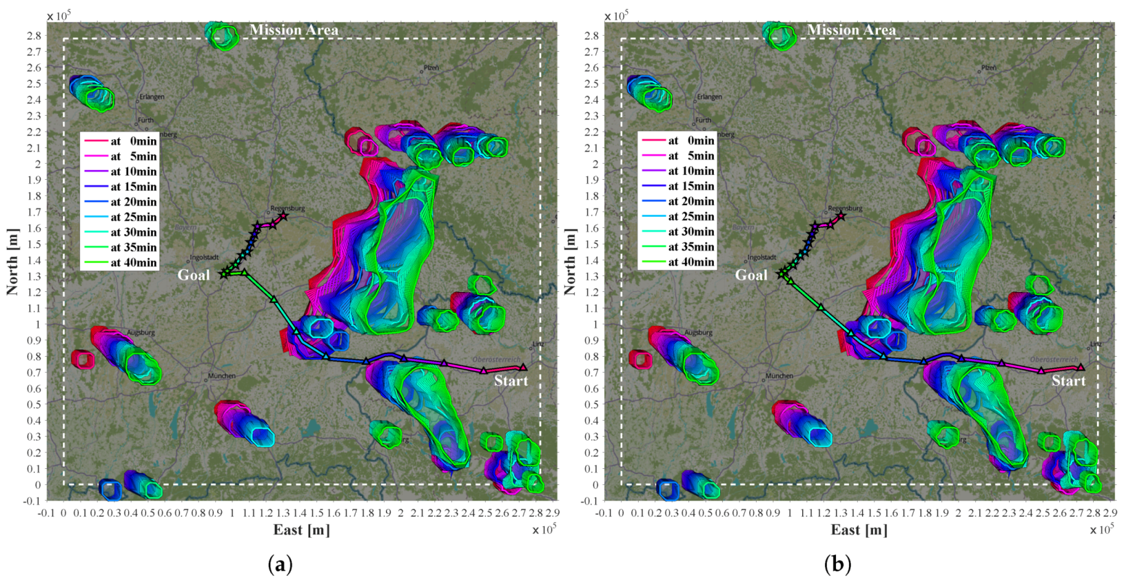
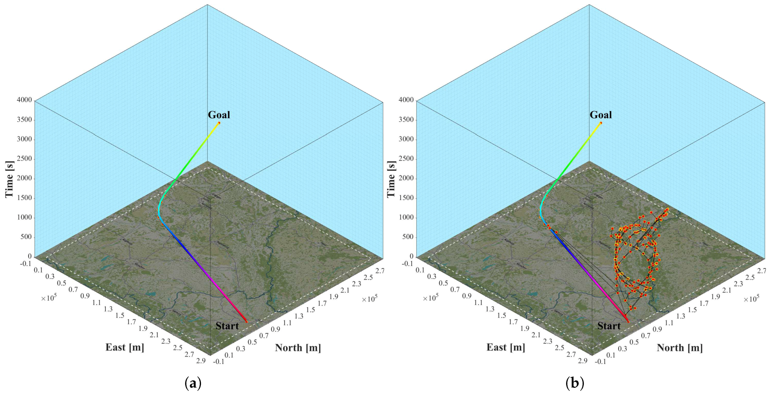
3.4. Moving Goal Scenario
Table 21 lists the values used for the simulation of an automatic holding pattern.
In Figure 15a, the actual position of the moving goal (colored star markers) is updated with every nowcast which results in a reactive navigation. In Figure 15b, the aircraft has the information about the future goal states in advance, which allows a tactical flight directly towards the estimated area of meeting.
4. Discussion
Comparing Figure 9a,b illustrates the considerable amount of prediction uncertainty the MPTP is subjected to. This manifests in the differences between the anticipatory trajectories (monochrome lines) in Figure 11 and Figure 12. Although solely relying on external information by nowcast, the MPTP safely avoids thunderstorms in all presented scenarios (Section 3.2, Section 3.3 and Section 3.4). The key is the implicit consideration of uncertainty by replanning a near-optimal anticipatory trajectory for the expected case with every update of the nowcast.
Figure 10 illustrates that the planning is done in three-dimensions as time has to be considered in dynamic environments. The anticipatory nature of the trajectory is shown by the absence of pursuit curves. It is free of conflicts and the vertical slope is always positive, which means that time is monotonically increasing. Due to the constant the vertical slope is likewise constant.
The final trajectories from start state to goal in Scenario 1 and Scenario 2 are assembled by the first legs of the anticipatory trajectories with a duration of . As each of them is the best guess at the time, the final trajectory is in both scenarios shorter than expected in the first MPTP iteration. Probabilistic margins help to prevent the MPTP from replanning substantially diverging trajectories.
In Scenario 2, the goal lies in the direction of the moving thunderstorms (Figure 12). At 19:05 h, the thunderstorms are moving at a ground speed ranging from m/s to m/s and a mean of m/s with to and a mean of direction from north. The beeline between start and goal is km and almost in the opposite direction at . Although uncertainty is explicitly considered in the fourth MPTP iteration, the aircraft is suddenly inside a safety margin but still outside the cell itself (fourth and dark blue triangle from the start). A robust feature is the addition of the aircraft to if the aircraft is suddenly trapped. Thus, the algorithm is able to exit the conflict as fast as possible, while only marginally changing the course. This behavior is compliant with FAA rules [42]. Due to the fast development of thunderstorms, the nowcast uncertainty is sometimes so large that even extended probabilistic safety margins cannot completely rule out such incidents without excessive blockage of airspace. The only way to prevent this kind of unexpected incident is the availability of an onboard radar.
The results in Section 3.2 show that trajectory planning with unidirectional constrained turning is faster for all heuristics. This is intuitive as only one instead of two auxiliary states (Section 2.3.4) is added into the in each while loop of the A*-search. Although not evident from the presented results, the unidirectional constrained flight can lead to suboptimal trajectories due to unnecessary turning and even compromises convergence in some cases. However, it is important to keep the number of additional states in the as small as possible.
The performance of A*-search with three different heuristics is compared in Section 2.3.3. The ratio between the number of trajectory states (TRST) and the number of explored states (EXST) in order to compute the trajectory is taken as a criterion for effectiveness of the search.
If the heuristic cost H is set to zero, A* basically becomes Dijkstra’s algorithm. As expected, this results in the lowest ratios for TRST/EXST in all iterations of both scenarios. The reason is that the priority queue basically organizes the candidate states in ascending order regarding their G-cost. The uninformed search leads to the exploration of unnecessary candidate states. When bidirectional turning flight is allowed Dijkstra does not converge in hours which is why in both scenarios no data are presented. In this case, the minimum outdegree of each state is two. Therefore, the number of states to explore increases exponentially, which additionally slows down priority queue operations. As two newly added auxiliary states are near the actually explored state, they are high in the priority queue. This inhibits the progression of the search towards the goal. In Scenario 1, the TRST/EXST hit ratio for unidirectional turning is ≤2.2% when obstacles are in between start and goal (Table 5). In Scenario 2, the maximum allowed deviation is larger than in Scenario 1, which causes more candidate states in the . The TRST/EXST ratio in the first four MPTP iterations is extremely poor (Table 13). In the third MPTP iteration number of EXST is 15,830 times that of A*-search with SSPH (Table 16). These results indicate that Dijkstra is unsuitable for the present application in X-space.
The A* performs better with EDH as the search is informed. Without obstacles in between start and goal, the EXST/EXST ratio with EDH is on par with SSPH in uni- an bidirectional flight (see last MPTP iterations in Table 8, Table 11, Table 16 and Table 19). Although the pruning of nontangent edges in the prevents unnecessary candidate states, the search with EDH can be rather slow especially in crowded environments. The reason is that the beeline distance to the goal ignores obstacles. In unidirectional turning the unnecessary exploration of auxiliary states is inhibited by increasing values for Euclidean distance when performing a turn. This is why A* with EDH performs reasonably in both scenarios for unidirectional turning. In Scenario 1 (Table 8) A* with EDH explores at most 4.46 times more states than A* with SSPH and in Scenario 2 at most 38.5 times (Table 16). However, by adding left and right auxiliary states in every A* iteration, the inhibition of excessive exploration is abolished and the performance is unacceptable for the first MPTP iterations in Table 11 and Table 19. The search is unwilling to increase the H-cost in order to fly around obstacles and instead mainly explores the auxiliary states in front of the obstacles.
The A*-search with SSPH has the highest TRST/EXST hit rate in all MPTP iterations of both scenarios as obstacles are taken into account implicitly. As only the most promising states are explored, the performance between uni- and bidirectional turning flight is almost identical. Only in Scenario 1 in the first MPTP iteration the bidirectional search explores two states more than in the unidirectional case (compare Table 7 and Table 10). In Scenario 2, the number of EXST is identical for all MPTP iterations (compare Table 15 and Table 18). The introduced SSPH is not admissible as overestimation of the heuristic cost is possible, which is why the optimality of the trajectories cannot be guaranteed. This is due to the fact that SSPH is computed in the graph of free state space from the perspective of an initial state . Strictly speaking, the shape of the obstacles is only valid when staying on the radials outgoing from the initial state. As shortest paths for candidate states are evaluated around approximate obstacle shapes, under- as well as overestimation of the H-cost is possible. This mainly depends on the motion of obstacles relative to the shortest static path. If it passes on the side of movement direction the H-cost is underestimated. Underestimation slows the convergence yet leads to an optimal result and is therefore admissible. If the shortest path is on the backside of obstacle movement, the H-cost is overestimated which can lead to suboptimal results. However, overestimation of the H-cost is partly done on purpose by an inflation factor as this can speed up the search [57,58]. In Scenario 1, in the fourth iteration of the MPTP, the computed trajectory with SSPH (Table 7) is 200 m longer than with Dijkstra (Table 5) or A* with EDH (Table 6). Generally, if there is a difference between the trajectories, it is small. Compared to the large amount of nowcast uncertainty and extensive margins, these differences are negligible. The fact that Dijkstra and A*-search with EDH produce identical trajectories in 19 of the 20 presented anticipatory trajectories indicates that A* with SSPH frequently produces near-optimal results. Overall, the A*-search with SSPH is well-suited for planning in dynamic environment. It is considerably faster and more consistent compared to Dijkstra and A* with EDH. The runtime for trajectory planning is crucial for an online application. In Section 3, the aircraft travels at m/s. For example, in the first MPTP iteration in Scenario 2, the aircraft covers a distance of 80 m/s s = m using A* with SSPH vs. 80 m/s s m using A* with EDH while the trajectory is computed.
As it may not be possible to find a complete trajectory in an allotted time interval, an additional partial planning strategy is needed to avoid passivity [29] and guarantee decisioning. A possible strategy is to perform holdings in free state space. The example in Section 3.3 shows the ability of the planner to automatically plan holding patterns, e.g., if the goal is temporarily covered. This is important, as bounded margins (see Section 2.2.1) sometimes conservatively cover free space including the goal which reduces the probability of finding a solution. As before, the final trajectory takes less time than first guessed. Due to periodic replanning (Section 2.1) and estimation of future aircraft states (Section 2.2.2), the planner has the innate ability to deal with a moving goal (Section 3.4).
5. Conclusions
A method for robust trajectory planning in uncertain dynamic environments is presented. It enables anticipatory avoidance of static and moving obstacles. The shape and movement of the polygonal obstacles can be arbitrary. The combinatorial algorithm is resolution complete and near-time-optimal for the expected case under the assumption of constant true airspeed and angle of climb. The algorithm always performs the same computations and therefore the results are repeatable. Due to anticipatory planning and consideration of nonholonomic turning-flight constraint of fixed-wing aircraft, computed trajectories do not require postprocessing, as demonstrated in [4]. The ability to automatically plan holding patterns, if the goal itself or the access is covered by obstacles, improves the success rate of the planner.
The performance of A* search with three different heuristics was compared. Using A*-search with EDH provides the same results as Dijkstra’s algorithm but is much faster. A*-search with the introduced SSPH is faster than A* with EDH in all presented examples. This highly targeted heuristic enables fast and reliable combinatorial trajectory planning in state space. Although SSPH is not admissible and optimality cannot be guaranteed, the trajectories are near-optimal and mostly identical to those computed with Dijkstra or A*-search with EDH.
There is still room for improvement and open questions. An optimization and implementation of the algorithm in C/C++ will improve the runtime considerably. The MPTP is sensitive to certain parameters that influence the computational time and quality of the trajectories, e.g., the time step for the prediction and optimization. An automated selection of these parameters is necessary to get good results. Planned research will also include stochastic analysis regarding the reliability or success rates of the MPTP. Furthermore, an extension to four-dimensional trajectory planning using the fast marching method is intended. In addition, the ability to plan trajectories for multiple aircraft is on the agenda.
Funding
This research was funded as part of the Ludwig Bölkow Campus project StraVARIA by the Project Management Agency for Aeronautics Research and Technology of the Bavarian Ministry of Economic Affairs, Regional Development and Energy.
Acknowledgments
The author would like to thank his family and in alphabetical order of first names, Alexander Knoll, Alexander Weber, Ferdinand Settele, Marcus Kreuzer and Reiko Müller for their great support.
Conflicts of Interest
The author declares no conflict of interest. The funders had no role in the design of the study; in the collection, analyses, or interpretation of data; in the writing of the manuscript, or in the decision to publish the results.
References
- Jenamani, R.K.; Kumar, A. Bad weather and aircraft accidents—Global vis-à-vis Indian scenario. Curr. Sci. 2013, 104, 316–325. [Google Scholar]
- Fultz, A.J.; Ashley, W.S. Fatal weather-related general aviation accidents in the United States. Phys. Geogr. 2016, 37, 291–312. [Google Scholar] [CrossRef] [Green Version]
- Federal Aviation Administration. Circular Advisory: Clear Air Turbulence Avoidance; Federal Aviation Administration: Washington, DC, USA, 2016.
- Müller, R.; Kiam, J.J.; Mothes, F. Multiphysical simulation of a semi-autonomous solar powered high altitude pseudo-satellite. In Proceedings of the 2018 IEEE Aerospace Conference, Big Sky, MT, USA, 3–10 March 2018; pp. 1–16. [Google Scholar]
- Li, G.; Baker, S.P. Crash risk in general aviation. JAMA 2007, 297, 1596–1598. [Google Scholar] [CrossRef] [PubMed]
- Miller, G.A. The magical number seven, plus or minus two: Some limits on our capacity for processing information. Psychol. Rev. 1956, 63, 81. [Google Scholar] [CrossRef] [PubMed]
- De Lellis, E.; Morani, G.; Corraro, F.; Di Vito, V. On-line trajectory generation for autonomous unmanned vehicles in the presence of no-fly zones. Proc. Inst. Mech. Eng. Part G J. Aerosp. Eng. 2013, 227, 381–393. [Google Scholar] [CrossRef]
- Canny, J.; Donald, B.; Reif, J.; Xavier, P. On the complexity of kinodynamic planning. In Proceedings of the 1988 29th Annual Symposium on Foundations of Computer Science, White Plains, NY, USA, 24–26 October 1988. [Google Scholar]
- Donald, B.; Xavier, P.; Canny, J.; Reif, J. Kinodynamic motion planning. J. ACM 1993, 40, 1048–1066. [Google Scholar] [CrossRef]
- Stentz, A. The focussed D* algorithm for real-time replanning. IJCAI 1995, 95, 1652–1659. [Google Scholar]
- Leven, P.; Hutchinson, S. A framework for real-time path planning in changing environments. Int. J. Robot. Res. 2002, 21, 999–1030. [Google Scholar] [CrossRef]
- Mitchell, J.S. Geometric shortest paths and network optimization. In Handbook of Computational Geometry; CiteSeer: New York, NY, USA, 2000; Volume 334, pp. 633–702. [Google Scholar]
- Erdmann, M.; Lozano-Perez, T. On multiple moving objects. Algorithmica 1987, 2, 477. [Google Scholar] [CrossRef]
- LaValle, S.M. Planning Algorithms; Cambridge University Press: Cambridge, UK, 2006. [Google Scholar]
- Hentzen, D.; Kamgarpour, M.; Soler, M.; Gonzalez-Arribas, D. On maximizing safety in stochastic aircraft trajectory planning with uncertain thunderstorm development. Aerosp. Sci. Technol. 2018, 79, 543–553. [Google Scholar] [CrossRef] [Green Version]
- Summers, S.; Kamgarpour, M.; Lygeros, J.; Tomlin, C. A stochastic reach-avoid problem with random obstacles. In Proceedings of the 14th International Conference on Hybrid Systems: Computation and Control, Chicago, IL, USA, 12–14 April 2011; pp. 251–260. [Google Scholar]
- Bellman, R. Dynamic Programming; Princeton University Press: Princeton, NJ, USA, 1957. [Google Scholar]
- LaValle, S.M. Rapidly-Exploring Random Trees: A New Tool for Path Planning; Citeseer: New York, NY, USA, 1998. [Google Scholar]
- LaValle, S.M.; Kuffner, J.J., Jr. Rapidly-exploring random trees: Progress and prospects. In Algorithmic and Computational Robotics, New Directions: The Fourth Workshop on the Algorithmic Foundations of Robotics; A. K. Peters, Ltd.: Natick, MA, USA, 2001; pp. 293–308. [Google Scholar]
- LaValle, S.M.; Kuffner, J.J., Jr. Randomized kinodynamic planning. Int. J. Robot. Res. 2001, 20, 378–400. [Google Scholar] [CrossRef]
- Kindel, R.; Hsu, D.; Latombe, J.C.; Rock, S. Kinodynamic motion planning amidst moving obstacles. In Proceedings of the IEEE International Conference on Robotics and Automation, San Francisco, CA, USA, 24–28 April 2000; Volume 1, pp. 537–543. [Google Scholar]
- Petti, S.; Fraichard, T. Safe motion planning in dynamic environments. In Proceedings of the 2005 IEEE/RSJ International Conference on Intelligent Robots and Systems, Edmonton, AB, Canada, 2–6 August 2005; pp. 2210–2215. [Google Scholar]
- Elbanhawi, M.; Simic, M. Sampling-based robot motion planning: A review. IEEE Access 2014, 2, 56–77. [Google Scholar] [CrossRef]
- Schwartz, J.T.; Sharir, M. General Techniques for Computing Topological Properties of Real Algebraic Manifolds; Ablex Publishing Corporation: New York, NY, USA, 1983. [Google Scholar]
- Canny, J. The Complexity of Robot Motion Planning; MIT Press: Cambriage, MA, USA, 1988. [Google Scholar]
- Fujimura, K.; Samet, H. Planning a time-minimal motion among moving obstacles. Algorithmica 1993, 10, 41–63. [Google Scholar] [CrossRef]
- Van Den Berg, J.; Overmars, M. Planning time-minimal safe paths amidst unpredictably moving obstacles. Int. J. Robot. Res. 2008, 27, 1274–1294. [Google Scholar] [CrossRef]
- Hart, P.E.; Nilsson, N.J.; Raphael, B. A formal basis for the heuristic determination of minimum cost paths. IEEE Trans. Syst. Sci. Cybern. 1968, 4, 100–107. [Google Scholar] [CrossRef]
- Petti, S.; Fraichard, T. Partial motion planning framework for reactive planning within dynamic environments. In Proceedings of the IFAC/AAAI International Conference on Informatics in Control, Automation and Robotics, Barcelona, Spain, 14–17 Setember 2005. [Google Scholar]
- Bottasso, C.L.; Leonello, D.; Savini, B. Path planning for autonomous vehicles by trajectory smoothing using motion primitives. IEEE Trans. Control Syst. Technol. 2008, 16, 1152–1168. [Google Scholar] [CrossRef]
- Bittner, M. Utilization of Problem and Dynamic Characteristics for Solving Large Scale Optimal Control Problems. Ph.D. Thesis, Technische Universität München, München, Germany, 2017. [Google Scholar]
- Marconnet, D.; Norden, C.; Vidal, L. Optimum use of weather radar. Saf. First 2016, 22, 22–43. [Google Scholar]
- Frazzoli, E.; Dahleh, M.A.; Feron, E. Real-time motion planning for agile autonomous vehicles. J. Guid. Control. Dyn. 2002, 25, 116–129. [Google Scholar] [CrossRef]
- Falcone, P.; Borrelli, F.; Tseng, H.E.; Asgari, J.; Hrovat, D. A hierarchical model predictive control framework for autonomous ground vehicles. In Proceedings of the 2008 American Control Conference, Seattle, WA, USA, 11–13 June 2008; pp. 3719–3724. [Google Scholar]
- Kober, K.; Tafferner, A. Tracking and nowcasting of convective cells using remote sensing data from radar and satellite. Meteorol. Z. 2009, 18, 75–84. [Google Scholar] [CrossRef] [Green Version]
- Mirza, A.; Pagé, C.; Geindre, S. FLYSAFE—An approach to safety—Using GML/XML objects to define hazardous volumes of aviation space. In Proceedings of the 13th Conference on Aviation, Range, and Aerospace Meteorology, New Orleans, LA, USA, 20–24 January 2008. [Google Scholar]
- Baldauf, M.; Förstner, J.; Klink, S.; Reinhardt, T.; Schraff, C.; Seifert, A.; Stephan, K.; Wetterdienst, D. Kurze Beschreibung des Lokal-Modells Kürzestfrist COSMO-DE (LMK) und seiner Datenbanken auf dem Datenserver des DWD; Deutscher Wetterdienst: Offenbach, Germany, 2014. [Google Scholar]
- Köhler, M.; Funk, F.; Gerz, T.; Mothes, F.; Stenzel, E. Comprehensive weather situation map based on XML-format as decision support for UAVs. J. Unman. Syst. Technol. 2017, 5, 13–23. [Google Scholar]
- Federal Aviation Administration. Circular Advisory: Thunderstorms; Federal Aviation Administration: Washington, DC, USA, 2013.
- Slingo, J.; Palmer, T. Uncertainty in weather and climate prediction. Philos. Trans. R. Soc. A Math. Phys. Eng. Sci. 2011, 369, 4751–4767. [Google Scholar] [CrossRef] [PubMed]
- Sauer, M.; Hauf, T.; Forster, C. Uncertainty Analysis of Thunderstorm Nowcasts for Utilization in Aircraft Routing. In Proceedings of the 4th SESAR Innovation Days (SID2014), Madrid, Spain, 25–27 November 2014; pp. 1–8. [Google Scholar]
- Federal Aviation Administration, Safety Team. Thunderstorms—Don’t Flirt...Skirt’Em; Federal Aviation Administration, Safety Team: Washington, DC, USA, 2008.
- Ester, M.; Kriegel, H.P.; Sander, J.; Xu, X. A density-based algorithm for discovering clusters in large spatial databases with noise. In Proceedings of the Second International Conference on Knowledge Discovery and Data Mining, Portland, OR, USA, 2–4 August 1996; pp. 226–231. [Google Scholar]
- Mothes, F.; Knoll, A. Automatische Wettervermeidung für ein unbemanntes, solarbetriebenes Flugzeug. In Proceedings of the German Aerospace Congress, Darmstadt, Germany, 30 September–2 October 2017. [Google Scholar]
- Osher, S.; Sethian, J.A. Fronts propagating with curvature-dependent speed: Algorithms based on Hamilton-Jacobi formulations. J. Comput. Phys. 1988, 79, 12–49. [Google Scholar] [CrossRef] [Green Version]
- Sethian, J.A. A fast marching level set method for monotonically advancing fronts. Proc. Natl. Acad. Sci. USA 1996, 93, 1591–1595. [Google Scholar] [CrossRef] [PubMed]
- Hassouna, M.S.; Farag, A.A. Multistencils fast marching methods: A highly accurate solution to the eikonal equation on cartesian domains. IEEE Trans. Pattern Anal. Mach. Intell. 2007, 29, 1563–1574. [Google Scholar] [CrossRef] [PubMed]
- Alton, K. Dijkstra-Like Ordered Upwind Methods for Solving Static Hamilton-Jacobi Equations. Ph.D. Thesis, University of British Columbia, Vancouver, BC, Canada, 2010. [Google Scholar]
- Elston, J.; Frew, E.W. Unmanned aircraft guidance for penetration of pretornadic storms. J. Guid. Control. Dyn. 2010, 33, 99–107. [Google Scholar] [CrossRef]
- Rohnert, H. Shortest paths in the plane with convex polygonal obstacles. Inf. Process. Lett. 1986, 23, 71–76. [Google Scholar] [CrossRef]
- Douglas, D.H.; Peucker, T.K. Algorithms for the reduction of the number of points required to represent a digitized line or its caricature. Cartogr. Int. J. Geogr. Inf. Geovis. 1973, 10, 112–122. [Google Scholar] [CrossRef]
- Prasad, D.K.; Leung, M.K.; Quek, C.; Cho, S.Y. A novel framework for making dominant point detection methods non-parametric. Image Vis. Comput. 2012, 30, 843–859. [Google Scholar] [CrossRef]
- Latombe, J.C. Robot Motion Planning: Edition en Anglais; Springer Science & Business Media: Berlin, Germany, 1991. [Google Scholar]
- Eriksson-Bique, S.; Kirkpatrick, D.; Polishchuk, V. Discrete dubins paths. arXiv 2012, arXiv:1211.2365. [Google Scholar]
- International Civil Aviation Organization ICAO. Aircraft Operations. Volume II, Construction of Visual and Instrument Flight Procedures; International Civil Aviation Organization ICAO: Montreal, QC, Canada, 2006. [Google Scholar]
- NATO Standardization Agency. STANAG 4586, 2nd ed.; ANNEX B; NATO Standardization Agency: Brussels, Belgium, 2007. [Google Scholar]
- Pohl, I. Heuristic search viewed as path finding in a graph. Artif. Intell. 1970, 1, 193–204. [Google Scholar] [CrossRef]
- Pearl, J. Heuristics: Intelligent Search Strategies for Computer Problem Solving; Addison-Wesley Pub. Co., Inc.: Reading, MA, USA, 1984. [Google Scholar]
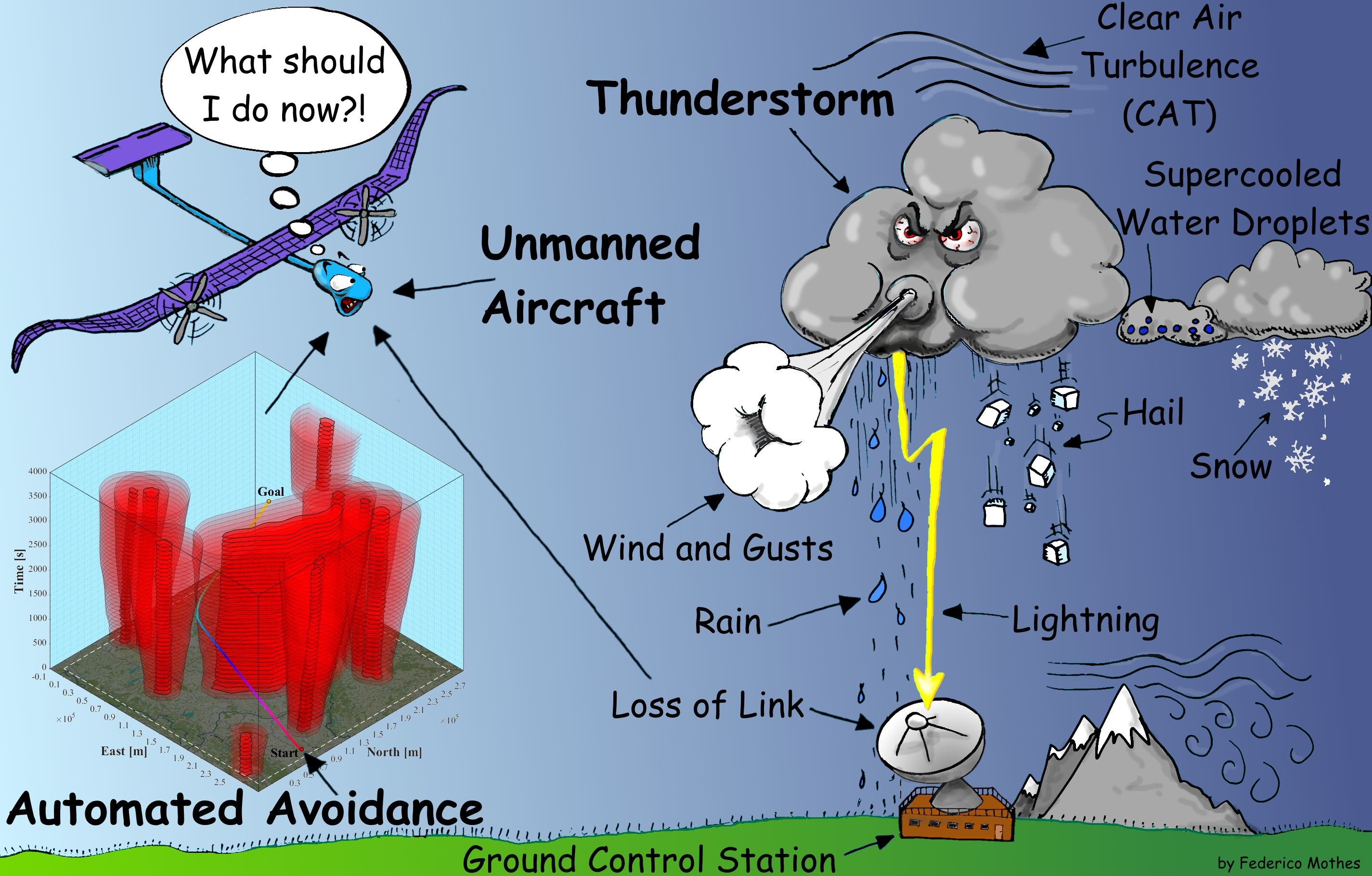
Figure 1.
Schematic of the presented MPTP and its environment. The update rate is five minutes.
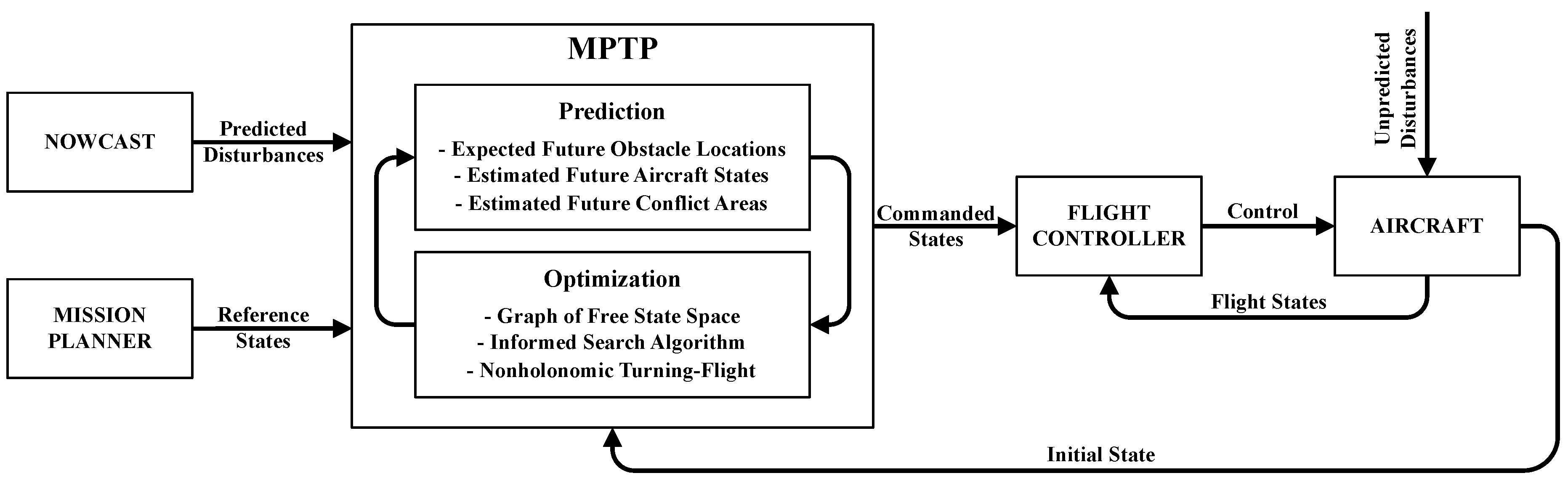
Figure 2.
Future states are depicted by yellow aircraft symbols. The isochronous progress with m/s is shown with black lines for s and s. (a) The results of the flight simulation with a maximum bank angle of compared to (b) approximated states.
Figure 2.
Future states are depicted by yellow aircraft symbols. The isochronous progress with m/s is shown with black lines for s and s. (a) The results of the flight simulation with a maximum bank angle of compared to (b) approximated states.

Figure 3.
In this example the ground speed is equal to true airspeed. The evolution of estimated conflict areas is illustrated at six points in time (–). For each time, the estimated future states (highlighted isochrone circle) in conflict with contemporaneous expected thunderstorms (varying polygon shapes) are marked in red. This results in the final shape of the ECAs shown at .

Figure 4.
In the anisotropic case, the groundspeed is not equal to true airspeed and depends on the aircraft’s position and course. The inhomogeneous gridded wind data are taken from a GRIB file (see Section 2.2.1). When considering wind the resulting ECAs differ noticeably from those in Figure 3.
Figure 4.
In the anisotropic case, the groundspeed is not equal to true airspeed and depends on the aircraft’s position and course. The inhomogeneous gridded wind data are taken from a GRIB file (see Section 2.2.1). When considering wind the resulting ECAs differ noticeably from those in Figure 3.

Figure 5.
The s (magenta surfaces) for a 3D thunderstorm cloud and its margin (translucent red volume) are shown for climb, level flight and descent.
Figure 5.
The s (magenta surfaces) for a 3D thunderstorm cloud and its margin (translucent red volume) are shown for climb, level flight and descent.
Figure 6.
(a) Unreduced; (b) reduced complete; and (c) reduced partial . The initial state and goal state are depicted by black diamonds.
Figure 6.
(a) Unreduced; (b) reduced complete; and (c) reduced partial . The initial state and goal state are depicted by black diamonds.
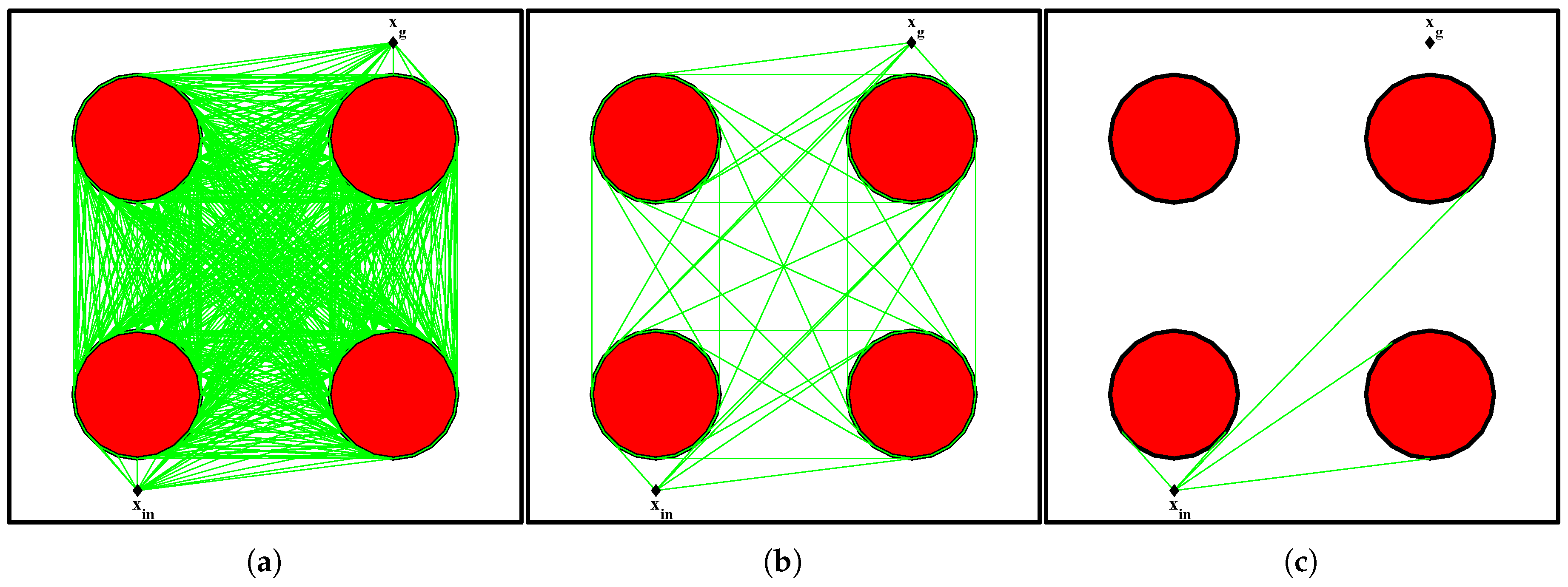
Figure 7.
Normalized aircraft covered distance and normalized minimum stabilization distance, when is performed (a) as fly-by or (b) as fly-over state.
Figure 7.
Normalized aircraft covered distance and normalized minimum stabilization distance, when is performed (a) as fly-by or (b) as fly-over state.
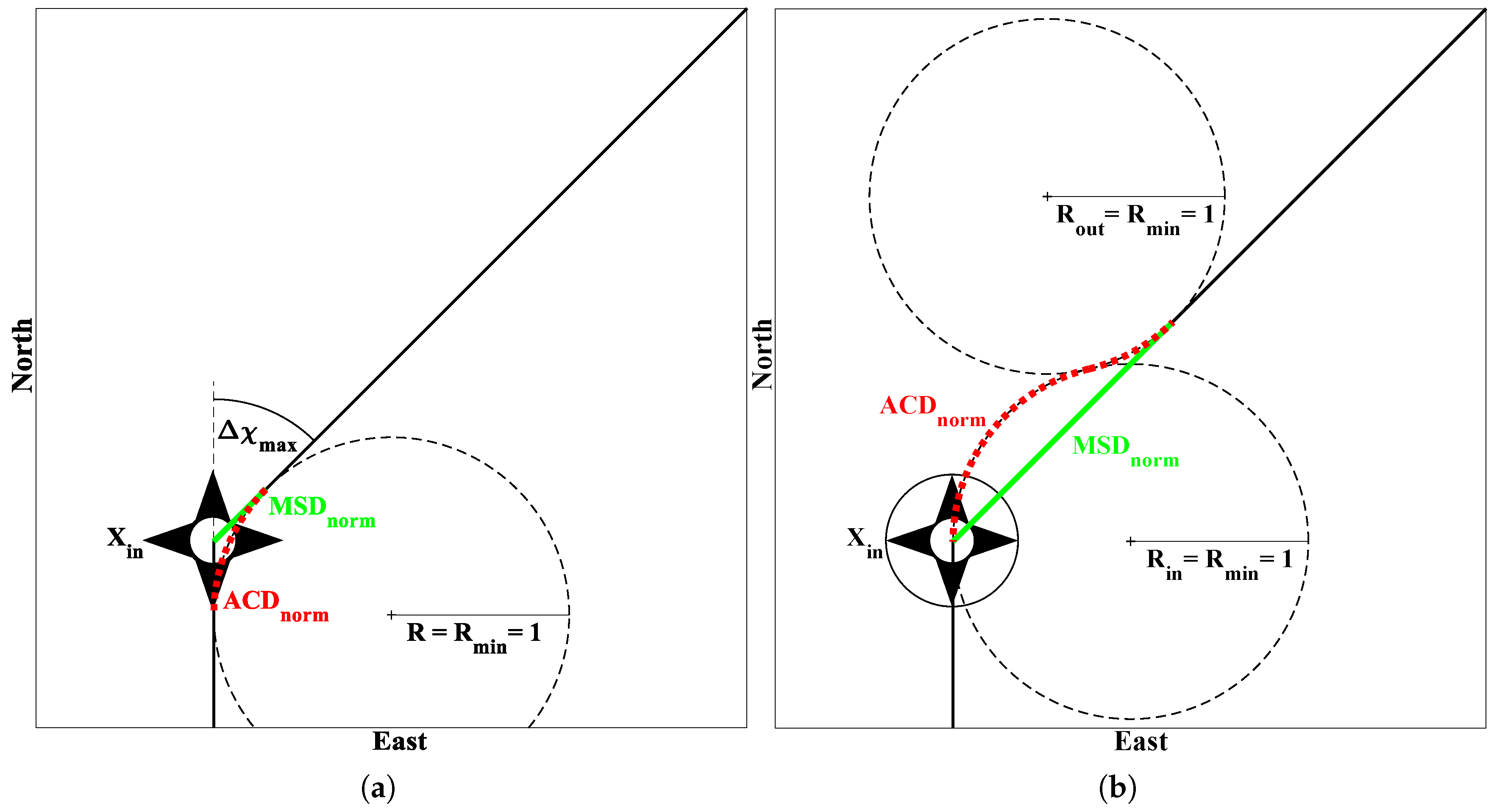
Figure 8.
Circular holding pattern defined by eight fly-over states.

Figure 9.
(a) Thunderstorm prediction by the nowcast issued 19:05 h for the next hour; and (b) subsequent real measurements for the same period of time, both issued by Rad-TRAM.
Figure 9.
(a) Thunderstorm prediction by the nowcast issued 19:05 h for the next hour; and (b) subsequent real measurements for the same period of time, both issued by Rad-TRAM.
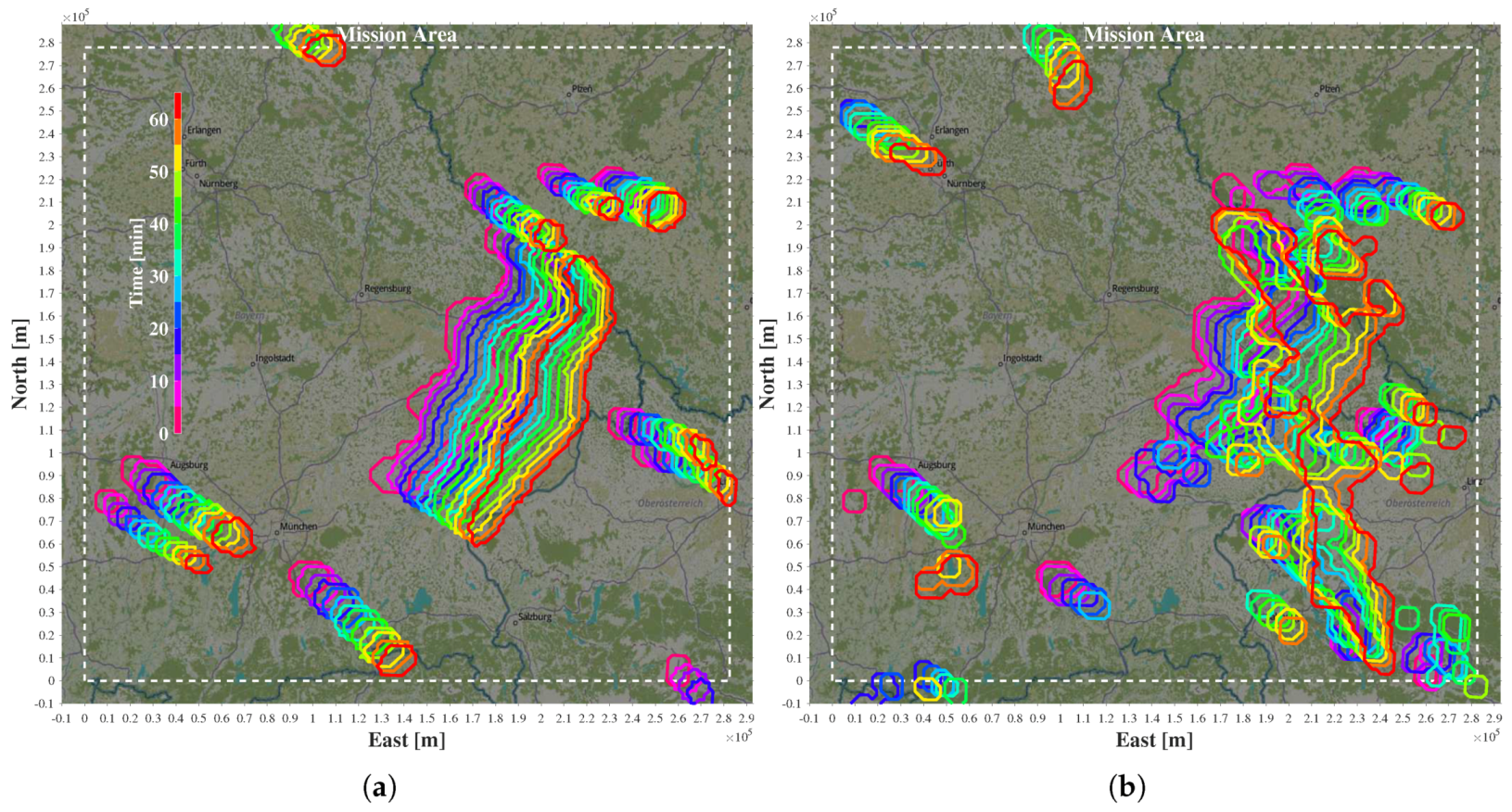
Figure 10.
Near-optimal anticipatory avoidance trajectory based on 19:05 h nowcast.
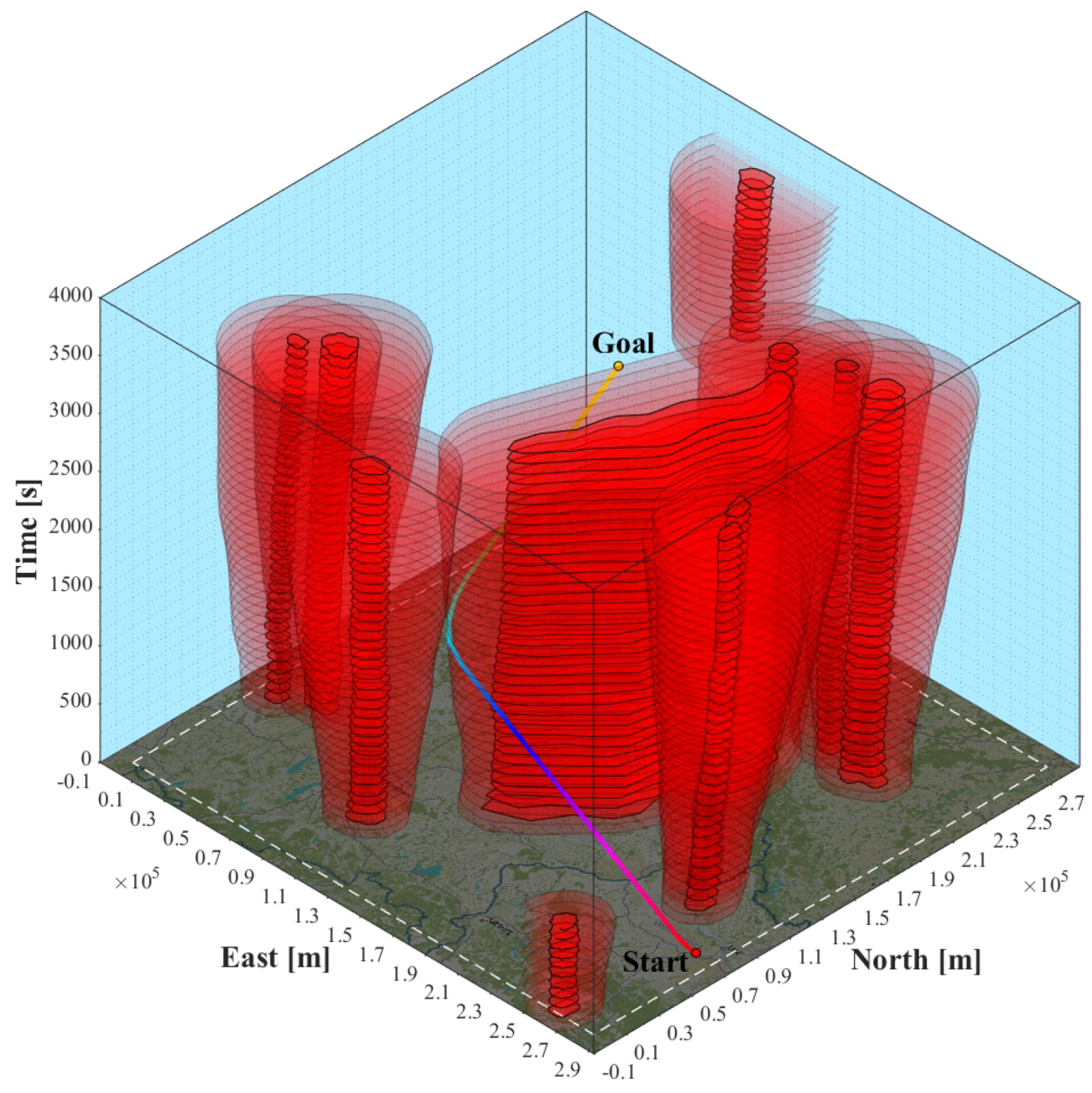
Figure 11.
(a) Continuous avoidance using SSPH. (b) Continuous avoidance using EDH. The runtimes for the MPTP iterations are listed in the respective legends.
Figure 11.
(a) Continuous avoidance using SSPH. (b) Continuous avoidance using EDH. The runtimes for the MPTP iterations are listed in the respective legends.
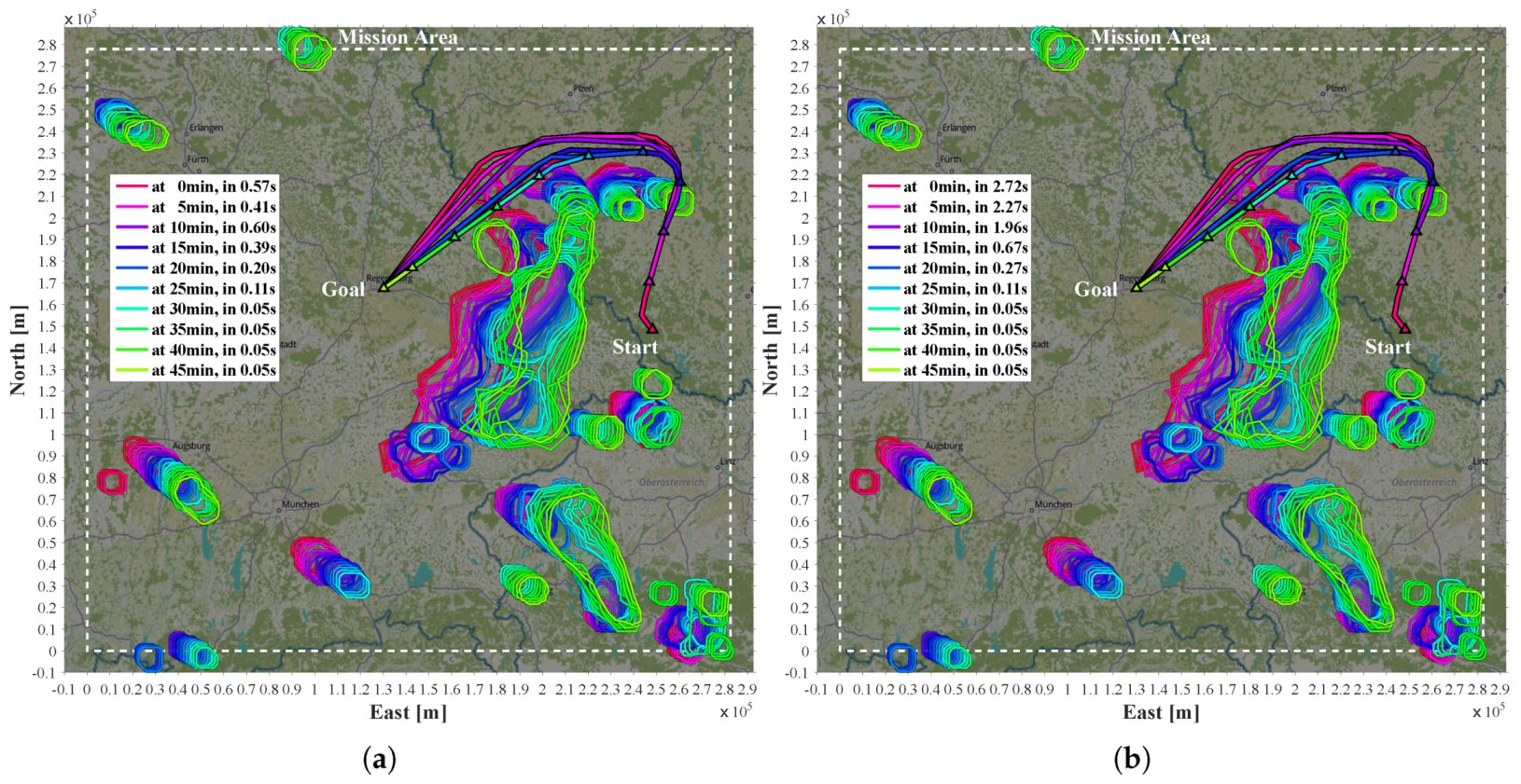
Figure 12.
(a) Continuous avoidance using SSPH. (b) Continuous avoidance using EDH.
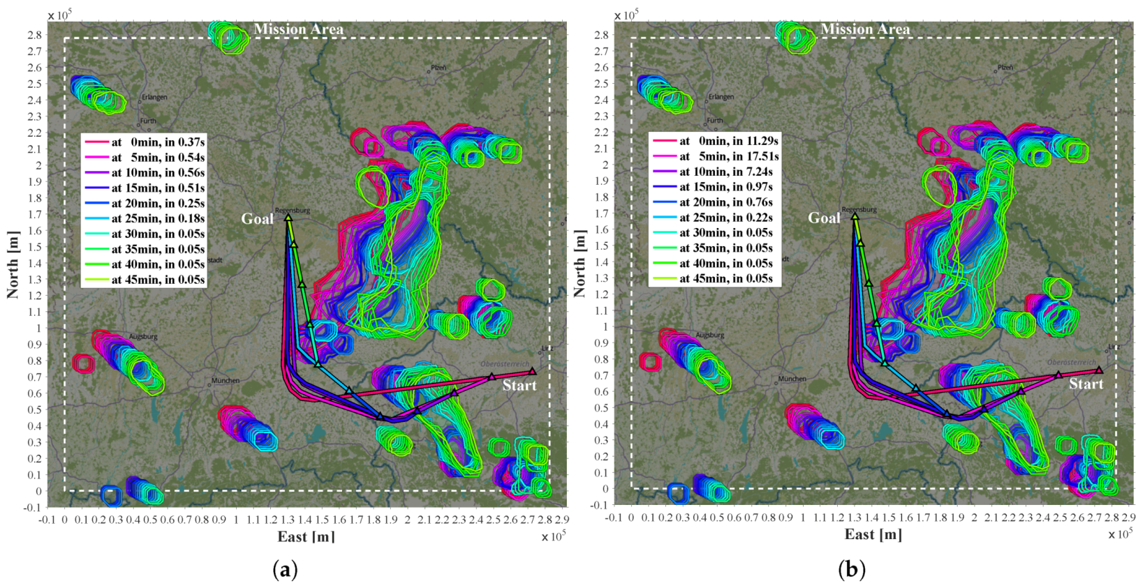
Figure 13.
Comparison for the first MPTP iteration in Tables 14 and 15: candidate future states (yellow and red dots) in the Closed List using (a) A* with SSPH and (b) A* with EDH. Until the goal is reached, the A*-like algorithm incrementally generates ramifications in the X-space all rooted in the start state.

Figure 14.
(a) Anticipatory trajectories including automatic holding patterns with runtimes for the MPTP iterations in the legend. (b) First iteration of the MPTP at in three dimensions. The static goal is indicated by a white line. As soon as the goal is uncovered, it is approached.
Figure 14.
(a) Anticipatory trajectories including automatic holding patterns with runtimes for the MPTP iterations in the legend. (b) First iteration of the MPTP at in three dimensions. The static goal is indicated by a white line. As soon as the goal is uncovered, it is approached.
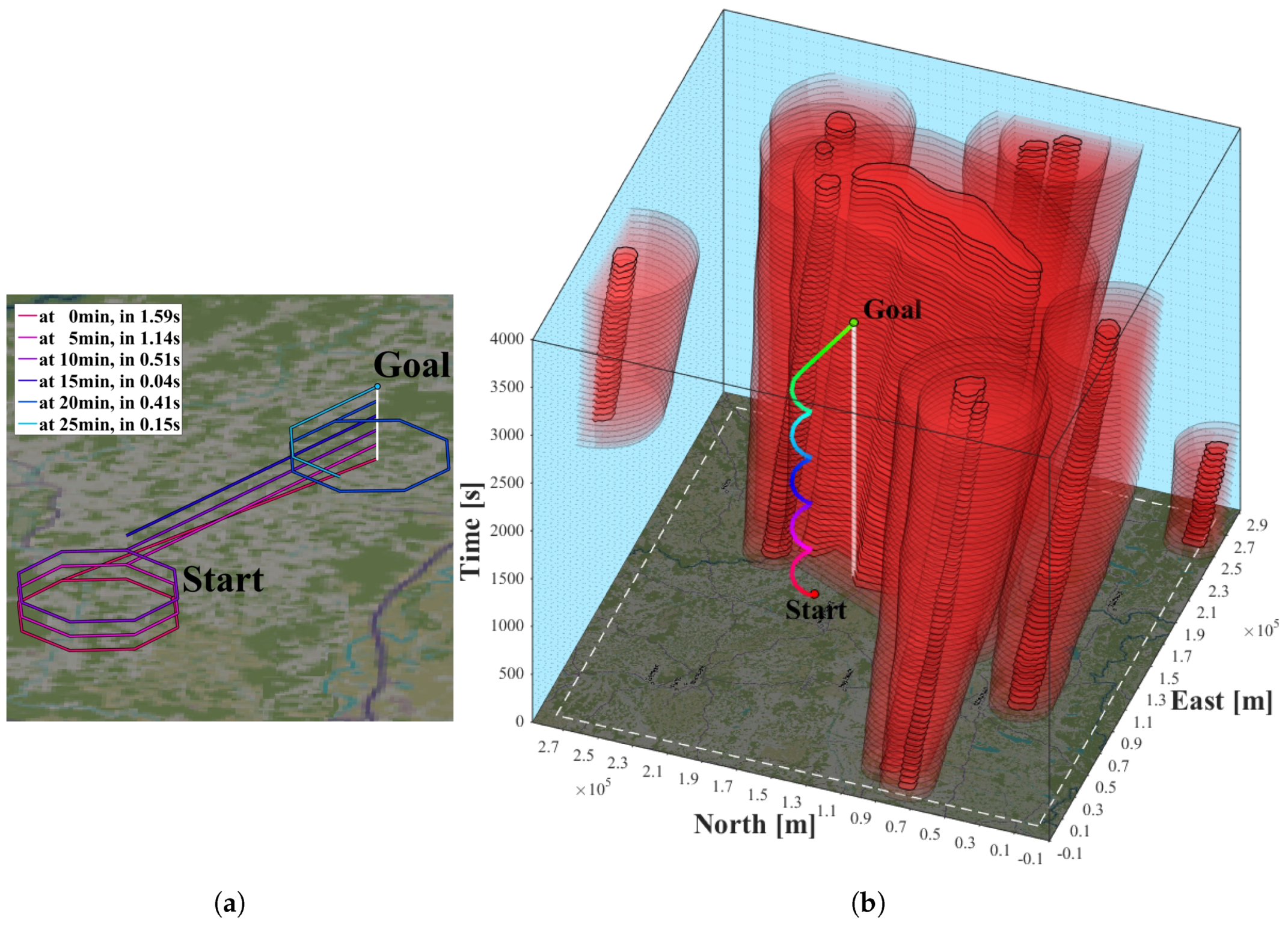
Figure 15.
(a) Reactive trajectory and (b) anticipatory trajectory to a moving goal.

Table 1.
Normalized minimum stabilization distances and velocity correction factors as functions of for fly-by states.
Table 1.
Normalized minimum stabilization distances and velocity correction factors as functions of for fly-by states.
| 5 | 12 | 20 | 30 | 45 | 60 | 72 | |
| 0.044 | 0.105 | 0.176 | 0.268 | 0.414 | 0.577 | 0.727 | |
| 1.000 | 1.000 | 0.999 | 0.998 | 0.991 | 0.969 | 0.929 |
Table 2.
Normalized minimum stabilization distances and velocity correction factors as functions of for fly-over states.
Table 2.
Normalized minimum stabilization distances and velocity correction factors as functions of for fly-over states.
| 5 | 12 | 20 | 30 | 45 | 60 | 72 | |
| 0.210 | 0.503 | 0.829 | 1.220 | 1.749 | 2.189 | 2.463 | |
| 1.001 | 1.005 | 1.015 | 1.033 | 1.078 | 1.139 | 1.206 |
Table 3.
Values for minimum stabilization distances for m/s, (as used in Section 3) for different values of , for fly-over and fly-by states.
Table 3.
Values for minimum stabilization distances for m/s, (as used in Section 3) for different values of , for fly-over and fly-by states.
| [] | 5 | 10 | 15 | 20 | 25 | 30 | 35 | 40 | 45 |
| [m] | 15091 | 7488 | 4928 | 3628 | 2831 | 2287 | 1886 | 1574 | 1320 |
| [m] | 3033 | 1505 | 990 | 729 | 569 | 459 | 379 | 316 | 265 |
Table 4.
Index s stands for start state and index g for the goal state.
| 19:05 h | 100 s | 80 m/s | 2000 m |
Table 5.
Dijkstra applied to the avoidance in Figure 11, if the aircraft can only turn right.
Table 5.
Dijkstra applied to the avoidance in Figure 11, if the aircraft can only turn right.
| MPTP Iteration | 1 | 2 | 3 | 4 | 5 | 6 | 7 | 8 | 9 | 10 |
|---|---|---|---|---|---|---|---|---|---|---|
| Trajectory Length [km] | 247.0 | 219.6 | 192.6 | 159.5 | 134.5 | 108.6 | 84.80 | 61.70 | 38.60 | 15.40 |
| Trajectory States (TRST) | 13 | 11 | 9 | 9 | 2 | 2 | 1 | 1 | 1 | 1 |
| Explored States (EXST) | 628 | 710 | 996 | 420 | 230 | 96 | 115 | 8 | 5 | 2 |
| TRST/EXST Ratio [%] | 2.070 | 1.549 | 0.904 | 2.143 | 0.870 | 2.083 | 0.870 | 12.50 | 20.00 | 50.00 |
Table 6.
A* with EDH applied to the avoidance in Figure 11, if the aircraft can only turn right.
Table 6.
A* with EDH applied to the avoidance in Figure 11, if the aircraft can only turn right.
| MPTP Iteration | 1 | 2 | 3 | 4 | 5 | 6 | 7 | 8 | 9 | 10 |
|---|---|---|---|---|---|---|---|---|---|---|
| Trajectory Length [km] | 247.0 | 219.6 | 192.6 | 159.5 | 134.5 | 108.6 | 84.80 | 61.70 | 38.60 | 15.40 |
| Trajectory States (TRST) | 13 | 11 | 9 | 9 | 2 | 2 | 1 | 1 | 1 | 1 |
| Explored States (EXST) | 58 | 49 | 50 | 14 | 5 | 2 | 1 | 1 | 1 | 1 |
| TRST/EXST Ratio [%] | 22.41 | 22.45 | 18.00 | 64.29 | 40.00 | 100.0 | 100.0 | 100.0 | 100.0 | 100.0 |
Table 7.
A* with SSPH applied to the avoidance in Figure 11, if the aircraft can only turn right.
Table 7.
A* with SSPH applied to the avoidance in Figure 11, if the aircraft can only turn right.
| MPTP Iteration | 1 | 2 | 3 | 4 | 5 | 6 | 7 | 8 | 9 | 10 |
|---|---|---|---|---|---|---|---|---|---|---|
| Trajectory Length [km] | 247.0 | 219.6 | 192.6 | 159.7 | 134.5 | 108.6 | 84.80 | 61.70 | 38.60 | 15.40 |
| Trajectory States (TRST) | 13 | 11 | 9 | 6 | 2 | 2 | 1 | 1 | 1 | 1 |
| Explored States (EXST) | 13 | 11 | 14 | 6 | 3 | 2 | 1 | 1 | 1 | 1 |
| TRST/EXST Ratio [%] | 100.0 | 100.0 | 64.29 | 100.0 | 100.0 | 100.0 | 100.0 | 100.0 | 100.0 | 100.0 |
Table 8.
Ratio between explored states for Dijkstra vs. A* with SSPH and A* with EDH vs. A* with SSPH, if the aircraft can only turn right.
Table 8.
Ratio between explored states for Dijkstra vs. A* with SSPH and A* with EDH vs. A* with SSPH, if the aircraft can only turn right.
| MPTP Iteration | 1 | 2 | 3 | 4 | 5 | 6 | 7 | 8 | 9 | 10 |
|---|---|---|---|---|---|---|---|---|---|---|
| EXST(Dijkstra)/EXST(SSPH) | 48.31 | 64.55 | 71.14 | 70.00 | 76.67 | 48.00 | 115.0 | 8.000 | 5.000 | 2.000 |
| EXST(EDH)/EXST(SSPH) | 4.462 | 4.455 | 3.571 | 2.333 | 1.667 | 1.000 | 1.000 | 1.000 | 1.000 | 1.000 |
Table 9.
A* using EDH applied to the avoidance in Figure 11, if the aircraft can turn left and right.
Table 9.
A* using EDH applied to the avoidance in Figure 11, if the aircraft can turn left and right.
| MPTP Iteration | 1 | 2 | 3 | 4 | 5 | 6 | 7 | 8 | 9 | 10 |
|---|---|---|---|---|---|---|---|---|---|---|
| Trajectory Length [km] | 247.0 | 219.6 | 192.6 | 159.5 | 134.5 | 108.6 | 84.80 | 61.70 | 38.60 | 15.40 |
| Trajectory States (TRST) | 13 | 11 | 9 | 9 | 2 | 2 | 1 | 1 | 1 | 1 |
| Explored States (EXST) | 12159 | 1397 | 113 | 14 | 5 | 2 | 1 | 1 | 1 | 1 |
| TRST/EXST Ratio [%] | 0.107 | 0.787 | 7.964 | 64.29 | 40.00 | 100.0 | 100.0 | 100.0 | 100.0 | 100.0 |
Table 10.
A* using SSPH applied to the avoidance in Figure 11, if the aircraft can turn left and right.
Table 10.
A* using SSPH applied to the avoidance in Figure 11, if the aircraft can turn left and right.
| MPTP Iteration | 1 | 2 | 3 | 4 | 5 | 6 | 7 | 8 | 9 | 10 |
|---|---|---|---|---|---|---|---|---|---|---|
| Trajectory Length [km] | 247.0 | 219.6 | 192.6 | 159.7 | 134.5 | 108.6 | 84.80 | 61.70 | 38.60 | 15.40 |
| Trajectory States (TRST) | 13 | 11 | 9 | 6 | 2 | 2 | 1 | 1 | 1 | 1 |
| Explored States (EXST) | 15 | 11 | 14 | 6 | 3 | 2 | 1 | 1 | 1 | 1 |
| TRST/EXST Ratio [%] | 86.67 | 100.0 | 64.29 | 100.0 | 66.67 | 100.0 | 100.0 | 100.0 | 100.0 | 100.0 |
Table 11.
Ratio between explored states for A* with EDH vs. A* with SSPH, if the aircraft can turn left and right.
Table 11.
Ratio between explored states for A* with EDH vs. A* with SSPH, if the aircraft can turn left and right.
| MPTP Iteration | 1 | 2 | 3 | 4 | 5 | 6 | 7 | 8 | 9 | 10 |
|---|---|---|---|---|---|---|---|---|---|---|
| EXST(EDH)/EXST(SSPH) | 810.6 | 127.0 | 8.071 | 2.333 | 1.667 | 1.000 | 1.000 | 1.000 | 1.000 | 1.000 |
Table 12.
Index s stands for start state and index g for the goal state.
| 19:05 h | 100 s | 80 m/s | 3000 m |
Table 13.
Dijkstra applied to the avoidance in Figure 12, if the aircraft can only turn right.
Table 13.
Dijkstra applied to the avoidance in Figure 12, if the aircraft can only turn right.
| MPTP Iteration | 1 | 2 | 3 | 4 | 5 | 6 | 7 | 8 | 9 | 10 |
|---|---|---|---|---|---|---|---|---|---|---|
| Trajectory States (TRST) | 6 | 8 | 8 | 8 | 3 | 3 | 1 | 1 | 1 | 1 |
| Explored States (EXST) | 17,633 | 63,940 | 174,137 | 6960 | 768 | 145 | 24 | 19 | 6 | 3 |
| TRST/EXST Ratio [%] | 0.034 | 0.013 | 0.005 | 0.115 | 2.391 | 2.069 | 4.167 | 5.263 | 16.67 | 33.33 |
Table 14.
A* with EDH applied to the avoidance in Figure 12, if the aircraft can only turn right.
Table 14.
A* with EDH applied to the avoidance in Figure 12, if the aircraft can only turn right.
| MPTP Iteration | 1 | 2 | 3 | 4 | 5 | 6 | 7 | 8 | 9 | 10 |
|---|---|---|---|---|---|---|---|---|---|---|
| Trajectory States (TRST) | 6 | 8 | 8 | 8 | 3 | 3 | 1 | 1 | 1 | 1 |
| Explored States (EXST) | 231 | 346 | 145 | 18 | 13 | 4 | 1 | 1 | 1 | 1 |
| TRST/EXST Ratio [%] | 2.597 | 2.312 | 5.517 | 44.44 | 23.08 | 75.00 | 100.0 | 100.0 | 100.0 | 100.0 |
Table 15.
A* with SSPH applied to the avoidance in Figure 12, if the aircraft can only turn right.
Table 15.
A* with SSPH applied to the avoidance in Figure 12, if the aircraft can only turn right.
| MPTP Iteration | 1 | 2 | 3 | 4 | 5 | 6 | 7 | 8 | 9 | 10 |
|---|---|---|---|---|---|---|---|---|---|---|
| Trajectory States (TRST) | 6 | 8 | 8 | 8 | 3 | 3 | 1 | 1 | 1 | 1 |
| Explored States (EXST) | 6 | 10 | 11 | 9 | 4 | 3 | 1 | 1 | 1 | 1 |
| TRST/EXST Ratio [%] | 100.0 | 80.00 | 72.73 | 88.89 | 75.00 | 100.0 | 100.0 | 100.0 | 100.0 | 100.0 |
Table 16.
Ratio between explored states for Dijkstra vs. A* with SSPH and A* with EDH vs. A* with SSPH, if the aircraft can only turn right.
Table 16.
Ratio between explored states for Dijkstra vs. A* with SSPH and A* with EDH vs. A* with SSPH, if the aircraft can only turn right.
| MPTP Iteration | 1 | 2 | 3 | 4 | 5 | 6 | 7 | 8 | 9 | 10 |
|---|---|---|---|---|---|---|---|---|---|---|
| EXST(Dijkstra)/EXST(SSPH) | 2939 | 6394 | 15830 | 733.3 | 192.0 | 48.33 | 24.00 | 19.00 | 6.000 | 3.000 |
| EXST(EDH)/EXST(SSPH) | 38.50 | 34.60 | 13.18 | 2.000 | 3.250 | 1.333 | 1.000 | 1.000 | 1.000 | 1.000 |
Table 17.
A* with EDH applied to the avoidance in Figure 12, if the aircraft can turn left and right.
Table 17.
A* with EDH applied to the avoidance in Figure 12, if the aircraft can turn left and right.
| MPTP Iteration | 1 | 2 | 3 | 4 | 5 | 6 | 7 | 8 | 9 | 10 |
|---|---|---|---|---|---|---|---|---|---|---|
| Trajectory States (TRST) | 6 | 8 | 8 | 8 | 3 | 3 | 1 | 1 | 1 | 1 |
| Explored States (EXST) | 28,007 | 13,809 | 1267 | 67 | 19 | 5 | 1 | 1 | 1 | 1 |
| TRST/EXST Ratio [%] | 0.021 | 0.058 | 0.631 | 11.94 | 15.79 | 60.00 | 100.0 | 100.0 | 100.0 | 100.0 |
Table 18.
A* with SSPH applied to the avoidance in Figure 12, if the aircraft can turn left and right.
Table 18.
A* with SSPH applied to the avoidance in Figure 12, if the aircraft can turn left and right.
| MPTP Iteration | 1 | 2 | 3 | 4 | 5 | 6 | 7 | 8 | 9 | 10 |
|---|---|---|---|---|---|---|---|---|---|---|
| Trajectory States (TRST) | 6 | 8 | 8 | 8 | 3 | 3 | 1 | 1 | 1 | 1 |
| Explored States (EXST) | 6 | 10 | 11 | 9 | 4 | 3 | 1 | 1 | 1 | 1 |
| TRST/EXST Ratio [%] | 100.0 | 80.00 | 72.73 | 88.89 | 75.00 | 100.0 | 100.0 | 100.0 | 100.0 | 100.0 |
Table 19.
Ratio between explored states for A* with EDH vs. A* with SSPH, if the aircraft can turn left and right.
Table 19.
Ratio between explored states for A* with EDH vs. A* with SSPH, if the aircraft can turn left and right.
| MPTP Iteration | 1 | 2 | 3 | 4 | 5 | 6 | 7 | 8 | 9 | 10 |
|---|---|---|---|---|---|---|---|---|---|---|
| EXST(EDH)/EXST(SSPH) | 4668 | 1381 | 115.2 | 7.444 | 4.750 | 1.667 | 1.000 | 1.000 | 1.000 | 1.000 |
Table 20.
Index s stands for start state and index g for the goal state.
| 19:05 h | 60 s | 80 m/s | 2000 m |
Table 21.
Index s stands for start state and index g for the goal state.
| 19:05 h | 30 s | 80 m/s | 2000 m |
© 2019 by the author. Licensee MDPI, Basel, Switzerland. This article is an open access article distributed under the terms and conditions of the Creative Commons Attribution (CC BY) license (http://creativecommons.org/licenses/by/4.0/).
Share and Cite
MDPI and ACS Style
Mothes, F. Trajectory Planning in Time-Varying Adverse Weather for Fixed-Wing Aircraft Using Robust Model Predictive Control. Aerospace 2019, 6, 68. https://doi.org/10.3390/aerospace6060068
AMA Style
Mothes F. Trajectory Planning in Time-Varying Adverse Weather for Fixed-Wing Aircraft Using Robust Model Predictive Control. Aerospace. 2019; 6(6):68. https://doi.org/10.3390/aerospace6060068
Chicago/Turabian StyleMothes, Federico. 2019. "Trajectory Planning in Time-Varying Adverse Weather for Fixed-Wing Aircraft Using Robust Model Predictive Control" Aerospace 6, no. 6: 68. https://doi.org/10.3390/aerospace6060068
Note that from the first issue of 2016, this journal uses article numbers instead of page numbers. See further details here.