1. Introduction
Weather avoidance is an ever-present and safety-relevant task in manned and unmanned aviation. Approximately every fifth accident in commercial aviation and every fourth in general aviation is related to adverse weather [
1,
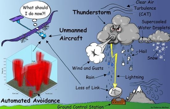
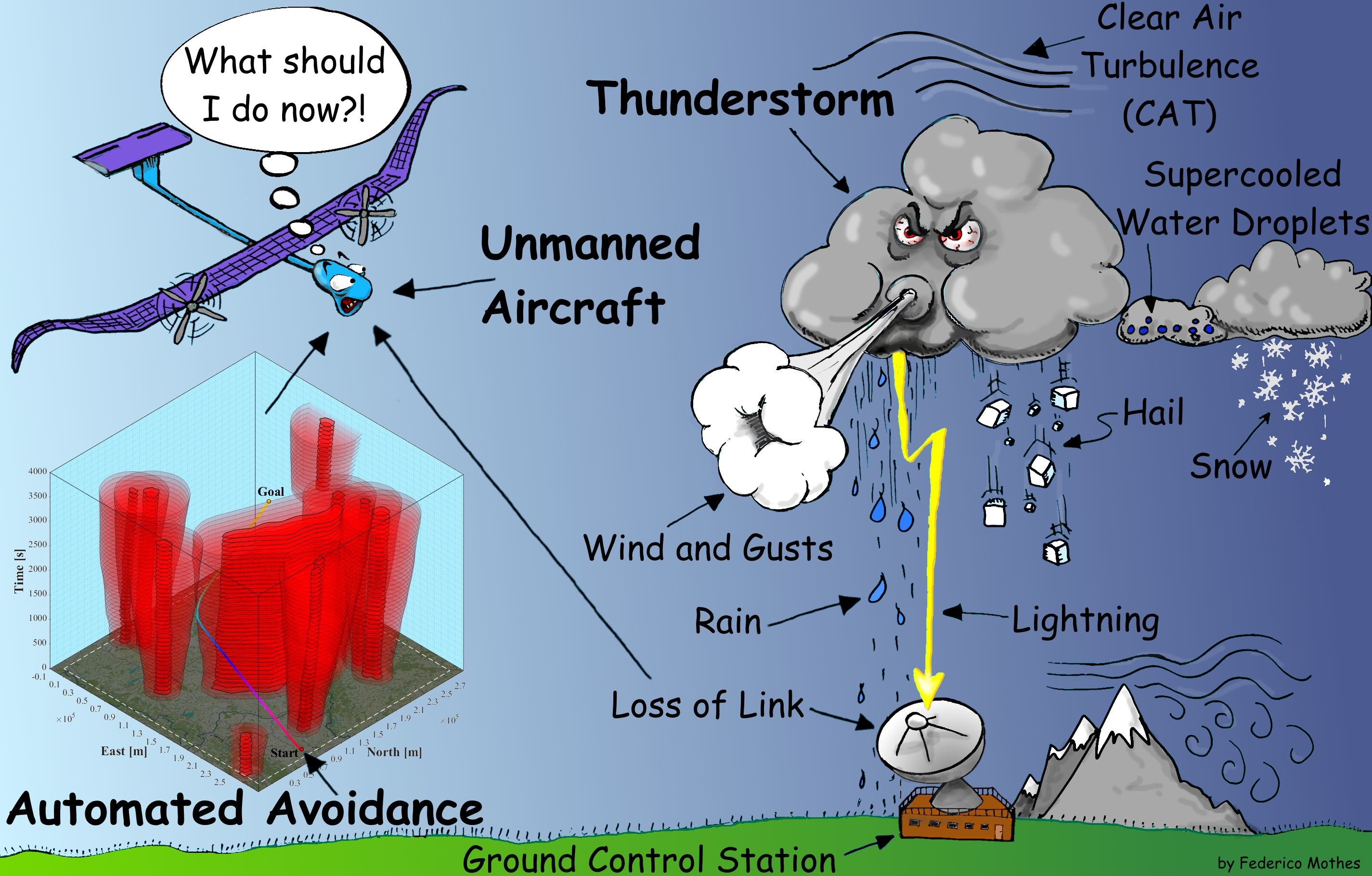
2]. Especially thunderstorms and their surroundings are dangerous, as turbulence, gusts, wind shear, lightning, hail and icing may occur. According to the Federal Aviation Administration (FAA), the philosophy of avoidance is an integral part of flight planning [
3]. This is especially true for light unmanned fixed-wing aircraft, for example high altitude pseudo-satellites [
4]. Their relatively low weight and performance increase the vulnerability to adverse weather [
5].
Thus far, the operation of these aircraft requires a considerable amount of manual effort in mission planning and execution. Many of the incurring tasks are related to tactical flight planning based on external meteorological information, as some aircraft are not equipped with an onboard weather radar. For this purpose, pilots and meteorologists have to consider a great amount of information all at once, i.e., actual and future aircraft states, airspace restrictions and time-variant forecasts under consideration of their uncertainty. However, memory capacity of humans is usually limited to 7 ± 2 chunks of information [
6], which is clearly insufficient to make optimal use of the available information. In complex scenarios with moving obstacles, this shortcoming can be partially compensated by applying quasi-static planning: Moving obstacles are avoided by an imaginary static radius of action plus an additional margin to account for uncertainty. This method works well when the aircraft is fast in relation to the obstacles. However, convective weather has a high rate of change and quasi-static avoidance is prone to cause reactive flight guidance. Reactive trajectories are suboptimal in terms of safety, mission accomplishment and energy consumption. For unmanned aircraft, a loss of link in both line of sight and beyond line of sight communication is a potential incident. The ability to continue flight in these situations, at least for a short period of time, enhances their level of autonomy and safety [
7]. The intrinsic complexity of anticipatory trajectory planning in uncertain dynamic environments calls for an automated solution. The consideration of kinematic and dynamic constraints further raises the complexity of this task [
8,
9].
The configuration
q of an aircraft is a combination of its degrees of freedom. The configuration space
C with
can be used for path planning in static environments. When dealing with moving obstacles, reactive planners use the static
C-space to perform replanning whenever the environment changes [
10,
11]. However, for anticipatory trajectory planning in the presence of moving obstacles, time has to be added to the
C-space. Therefore, even two-dimensional motion planning problems are difficult to solve as the dimensions are raised from two to three [
12]. A trajectory in this case is a path that is parameterized by monotonically increasing time and is compliant with kinematic and differential constraints of the aircraft. Erdmann and Lozano-Perez [
13] introduced the concept of configuration × time-space, which is also called state space (
X-space). Time-dependent configurations are called states
with
[
14]. Provided that a knowledge or estimate of the future obstacles exists, a sequence of states leading from start
to goal state
has to be determined. For this task, different motion planning methods exist.
An example for a control theory approach, regarding motion planning amid time-varying thunderstorms, is found in [
15]. A finite horizon reach-avoid problem formulation [
16] is used to maximize the probability of reaching a given point, while avoiding stochastic obstacles, under the consideration of uncertainties. Due to the curse of dimensionality [
17], this kind of approach is unsuitable for fast computation of problems with high degrees of freedom.
Classic robotic approaches for motion planning amid moving obstacles include sampling-based and combinatorial motion planning. Rapidly-exploring random trees (RRTs) belong to the family of sampling-based algorithms. They are extremely popular due to their ability to quickly find feasible trajectories in
X-space, for problems with high degrees of freedom and complicated constraints [
18,
19]. Examples for kinodynamic planning amidst moving obstacles can be found in [
20,
21,
22]. However, narrow passages can pose a problem, as the likelihood for a sample being in free space decreases. Furthermore, trajectories tend to be jerky and therefore require postprocessing, e.g., by B-splines, Bézier curves or clothoids [
23]. As random samples are used, the algorithm is probabilistically complete. This means that, if a trajectory exists and the number of samples approaches infinity, the probability to find the trajectory converges to one.
In [
8], a combinatorial method for kinodynamic planning is presented. The upper bound for the complexity of exact motion planning in a three-dimensional dynamic environment is given by a general algorithm with a time complexity that is double exponential in the dimension of search space [
24]. Canny [
25] introduced an algorithm where time complexity is only exponential in its dimension. A combinatorial motion planner searches a discrete topology of free space, e.g., a visibility graph, Voronoi diagram or an exact or approximate cell decomposition. The explicit representation of the search space limits the application of combinatorial methods to problems with low degrees of freedom, i.e., the number of parameters necessary to specify
q [
14]. Nonetheless, combinatorial planning offers desirable properties such as optimality, completeness and repeatable results that can be important for certification.
In this article, a combinatorial motion planner, called MPTP (see
Section 2.1), is described that computes collision-free, near-time-optimal and time-monotone trajectories from
to
similar to [
26,
27]. Global optimization is performed using an A*-search algorithm [
28]. Motion planning in the real-world is generally subject to uncertainty in environment and state predictability [
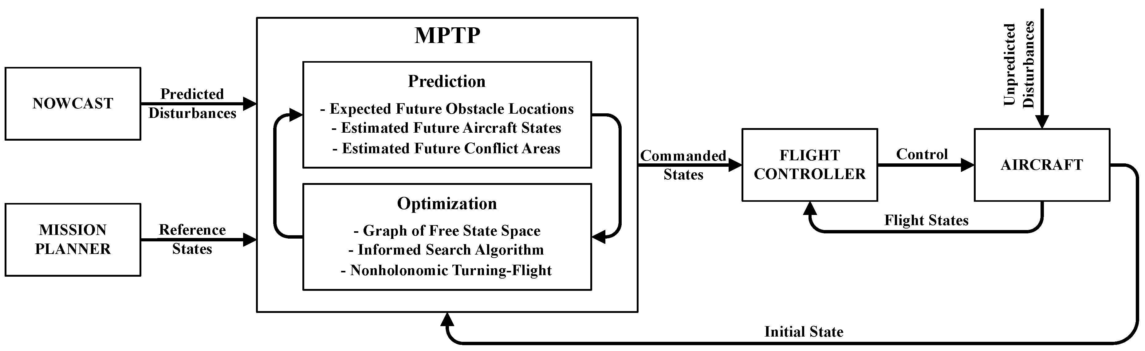
14]. In the presented setup, the planner solely relies on external environment prediction, in this case thunderstorm nowcasts. The immanent uncertainty in the environmental prediction is taken into account explicitly by bounded margins and implicitly by the closed loop of a model predictive controller (MPC). While planning takes place, information outdates in dynamic environments. This imposes a real-time decision constraint and limits the allotted time for trajectory planning [
29]. For fast convergence, the
X-space is iteratively built and its growth is restricted by a suitable heuristic. Furthermore, velocity and angle of climb are assumed to be at least piecewise constant. The planner uses a low-fidelity representation of aircraft dynamics with motion primitives. This ensures that the computed trajectories are compliant with the aircraft’s flight envelope and resulting tracking errors are small [
30].
The planner can be used as initial guess generator for gradient-based trajectory optimization in dynamic environments similar to Dubins path does in static environments to find an optimal control sequence in the homotopy class of the initial guess with a high-fidelity aircraft model [
14,
31].
The rest of this article is organized as follows. In
Section 2, the functional principle and technical details of the presented trajectory planner for dynamic environments are described.
Section 3 presents simulation results of the key capabilities, followed by the discussion (
Section 4) and conclusions (
Section 5).
4. Discussion
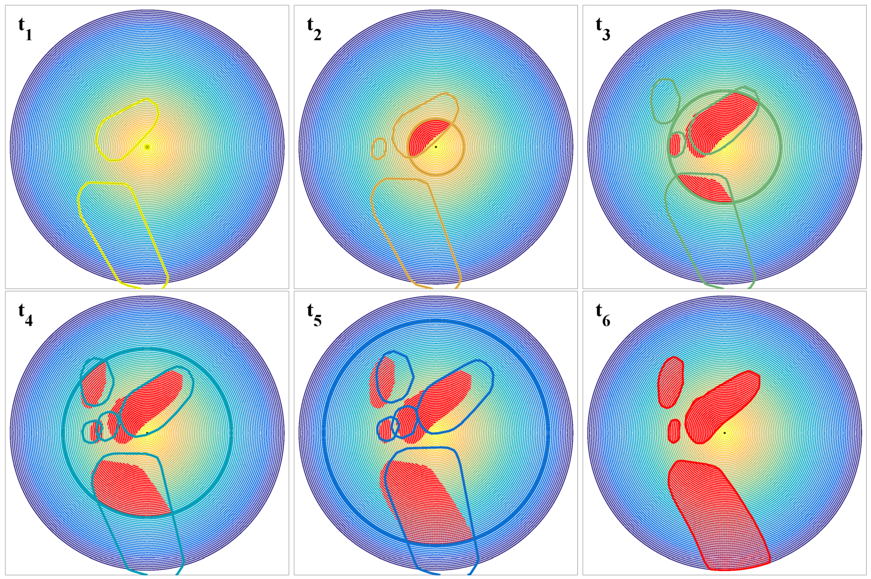
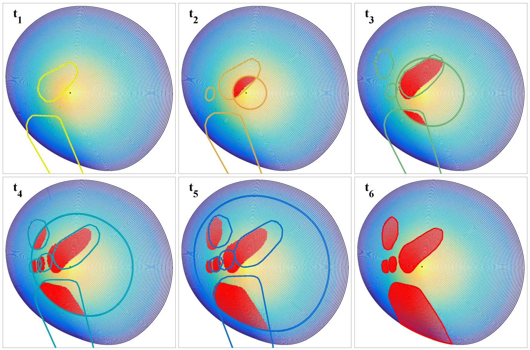
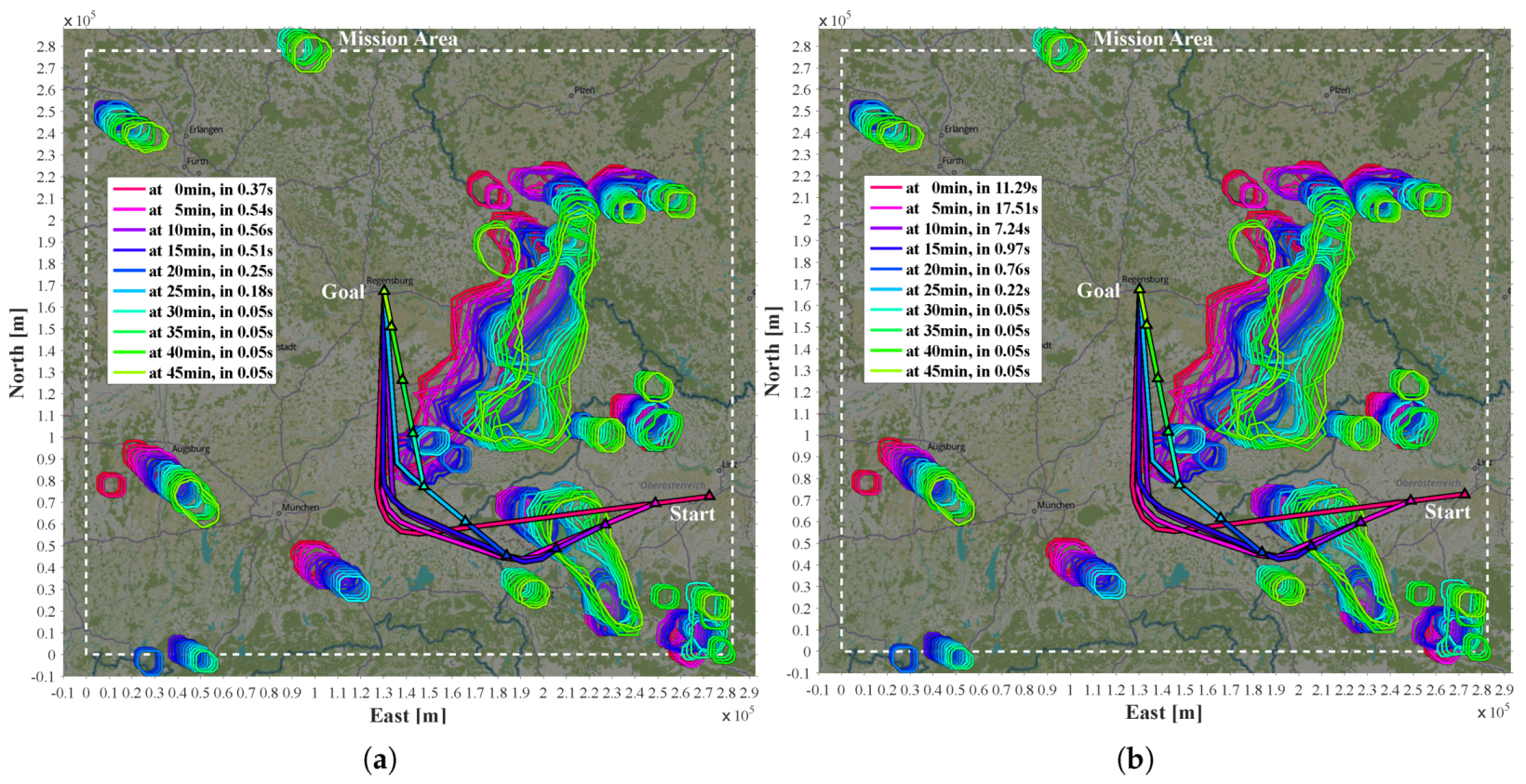
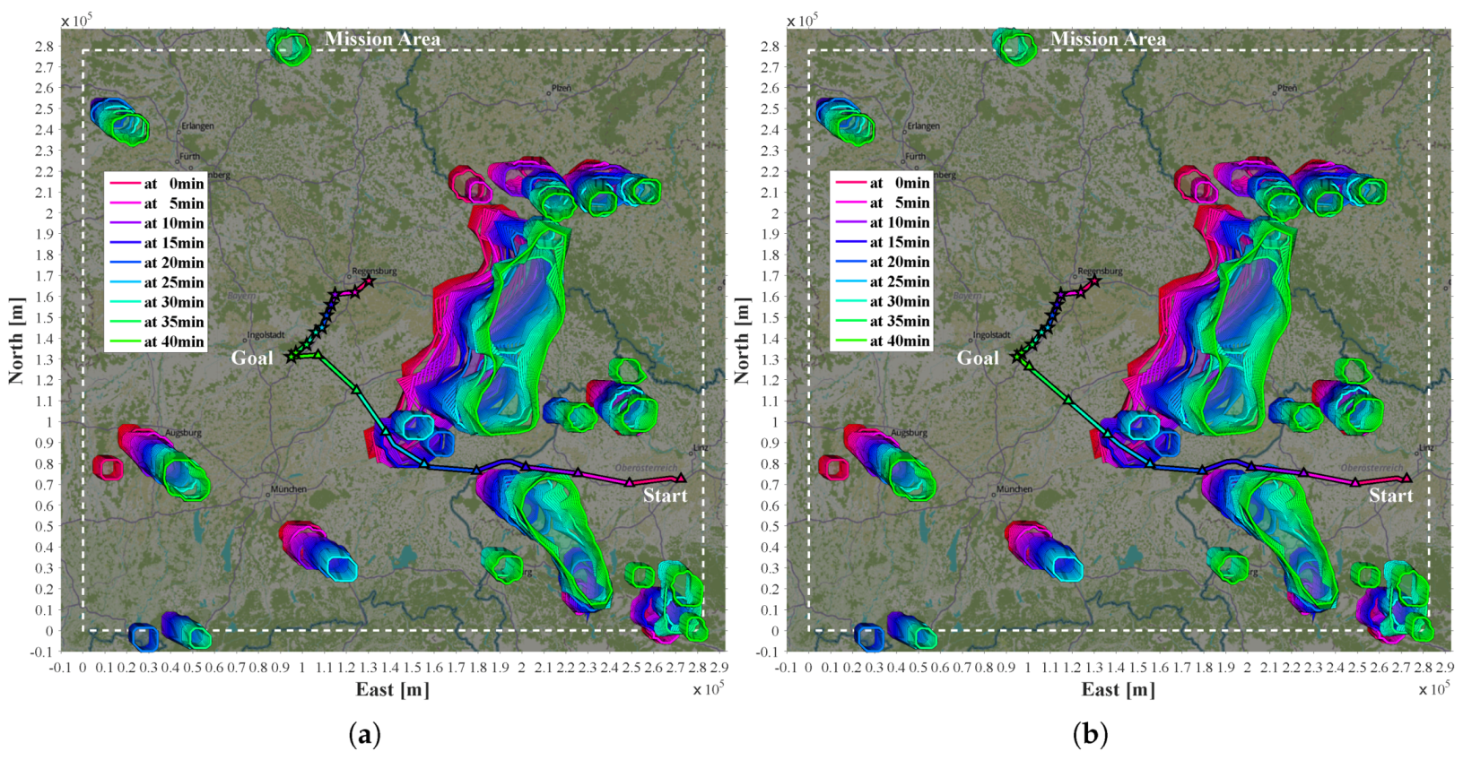
Comparing
Figure 9a,b illustrates the considerable amount of prediction uncertainty the MPTP is subjected to. This manifests in the differences between the anticipatory trajectories (monochrome lines) in
Figure 11 and
Figure 12. Although solely relying on external information by nowcast, the MPTP safely avoids thunderstorms in all presented scenarios (
Section 3.2,
Section 3.3 and
Section 3.4). The key is the implicit consideration of uncertainty by replanning a near-optimal anticipatory trajectory for the expected case with every update of the nowcast.
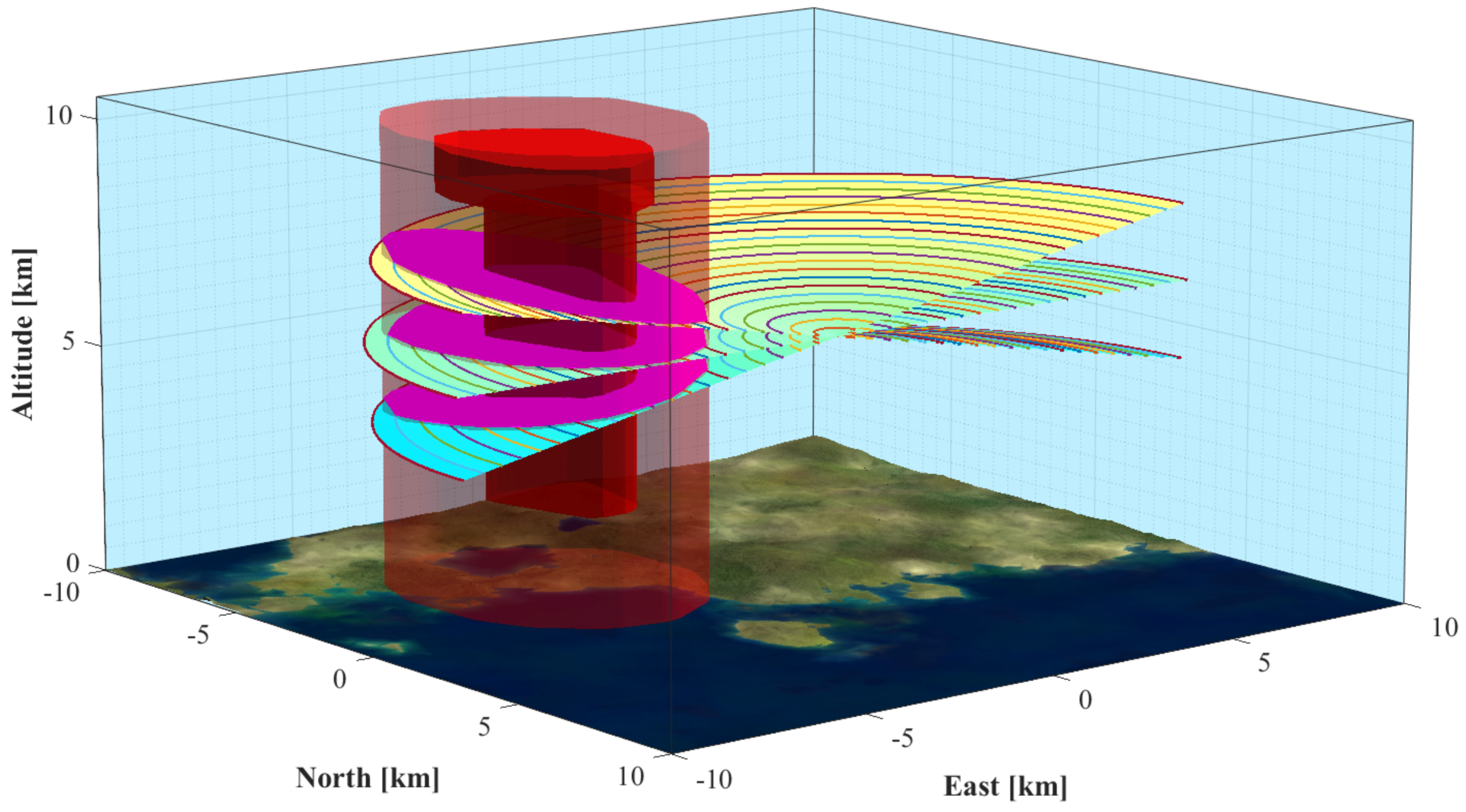
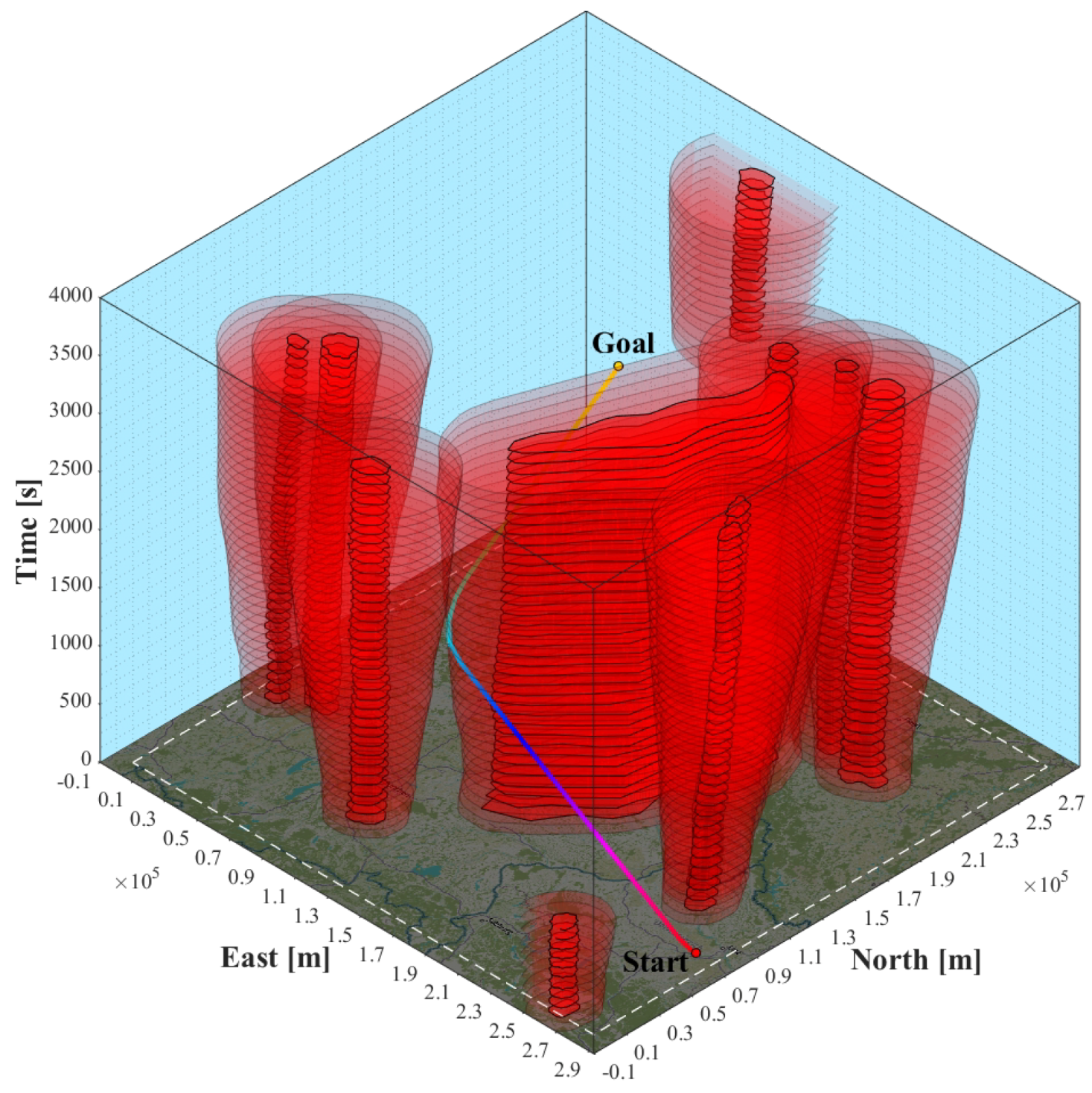
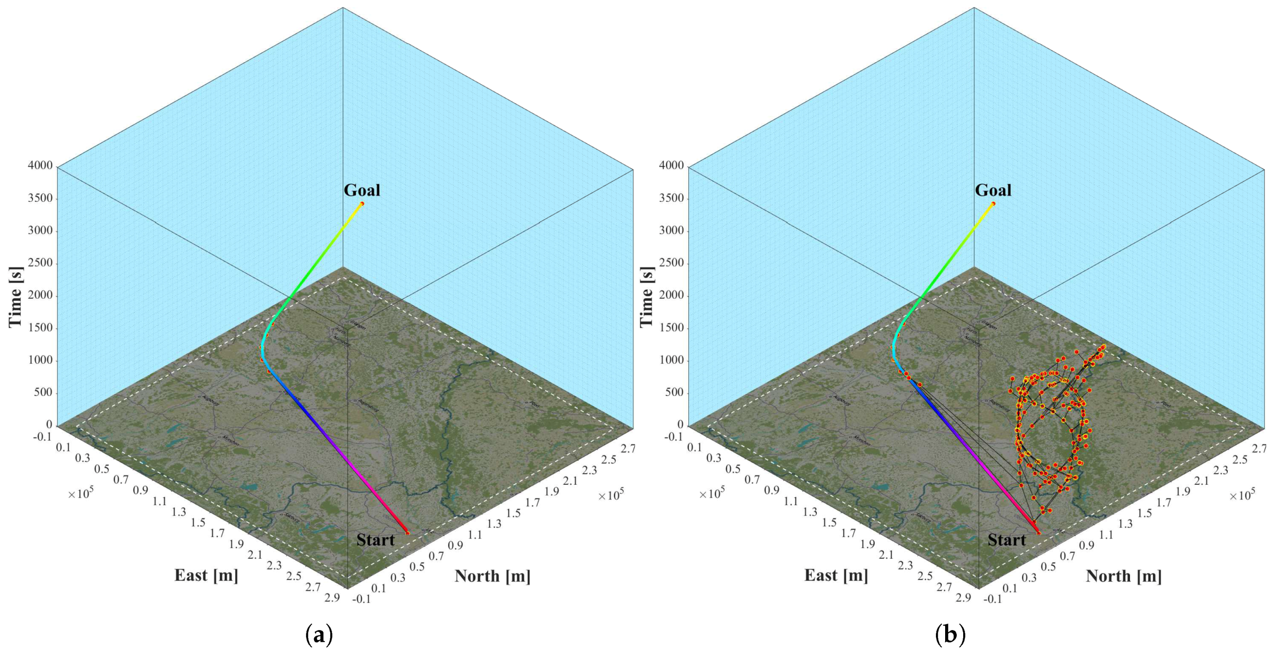
Figure 10 illustrates that the planning is done in three-dimensions as time has to be considered in dynamic environments. The anticipatory nature of the trajectory is shown by the absence of pursuit curves. It is free of conflicts and the vertical slope is always positive, which means that time is monotonically increasing. Due to the constant
the vertical slope is likewise constant.
The final trajectories from start state to goal in Scenario 1 and Scenario 2 are assembled by the first legs of the anticipatory trajectories with a duration of . As each of them is the best guess at the time, the final trajectory is in both scenarios shorter than expected in the first MPTP iteration. Probabilistic margins help to prevent the MPTP from replanning substantially diverging trajectories.
In Scenario 2, the goal lies in the direction of the moving thunderstorms (
Figure 12). At 19:05 h, the thunderstorms are moving at a ground speed ranging from
m/s to
m/s and a mean of
m/s with
to
and a mean of
direction from north. The beeline between start and goal is
km and almost in the opposite direction at
. Although uncertainty is explicitly considered in the fourth MPTP iteration, the aircraft is suddenly inside a safety margin but still outside the cell itself (fourth and dark blue triangle from the start). A robust feature is the addition of the aircraft to
if the aircraft is suddenly trapped. Thus, the algorithm is able to exit the conflict as fast as possible, while only marginally changing the course. This behavior is compliant with FAA rules [
42]. Due to the fast development of thunderstorms, the nowcast uncertainty is sometimes so large that even extended probabilistic safety margins cannot completely rule out such incidents without excessive blockage of airspace. The only way to prevent this kind of unexpected incident is the availability of an onboard radar.
The results in
Section 3.2 show that trajectory planning with unidirectional constrained turning is faster for all heuristics. This is intuitive as only one instead of two auxiliary states (
Section 2.3.4) is added into the
in each while loop of the A*-search. Although not evident from the presented results, the unidirectional constrained flight can lead to suboptimal trajectories due to unnecessary turning and even compromises convergence in some cases. However, it is important to keep the number of additional states in the
as small as possible.
The performance of A*-search with three different heuristics is compared in
Section 2.3.3. The ratio between the number of trajectory states (TRST) and the number of explored states (EXST) in order to compute the trajectory is taken as a criterion for effectiveness of the search.
If the heuristic cost
H is set to zero, A* basically becomes Dijkstra’s algorithm. As expected, this results in the lowest ratios for TRST/EXST in all iterations of both scenarios. The reason is that the priority queue basically organizes the candidate states in ascending order regarding their
G-cost. The uninformed search leads to the exploration of unnecessary candidate states. When bidirectional turning flight is allowed Dijkstra does not converge in hours which is why in both scenarios no data are presented. In this case, the minimum outdegree of each state is two. Therefore, the number of states to explore increases exponentially, which additionally slows down priority queue operations. As two newly added auxiliary states are near the actually explored state, they are high in the priority queue. This inhibits the progression of the search towards the goal. In Scenario 1, the TRST/EXST hit ratio for unidirectional turning is ≤2.2% when obstacles are in between start and goal (
Table 5). In Scenario 2, the maximum allowed deviation is larger than in Scenario 1, which causes more candidate states in the
. The TRST/EXST ratio in the first four MPTP iterations is extremely poor (
Table 13). In the third MPTP iteration number of EXST is 15,830 times that of A*-search with SSPH (
Table 16). These results indicate that Dijkstra is unsuitable for the present application in
X-space.
The A* performs better with EDH as the search is informed. Without obstacles in between start and goal, the EXST/EXST ratio with EDH is on par with SSPH in uni- an bidirectional flight (see last MPTP iterations in
Table 8,
Table 11,
Table 16 and
Table 19). Although the pruning of nontangent edges in the
prevents unnecessary candidate states, the search with EDH can be rather slow especially in crowded environments. The reason is that the beeline distance to the goal ignores obstacles. In unidirectional turning the unnecessary exploration of auxiliary states is inhibited by increasing values for Euclidean distance when performing a turn. This is why A* with EDH performs reasonably in both scenarios for unidirectional turning. In Scenario 1 (
Table 8) A* with EDH explores at most 4.46 times more states than A* with SSPH and in Scenario 2 at most 38.5 times (
Table 16). However, by adding left and right auxiliary states in every A* iteration, the inhibition of excessive exploration is abolished and the performance is unacceptable for the first MPTP iterations in
Table 11 and
Table 19. The search is unwilling to increase the
H-cost in order to fly around obstacles and instead mainly explores the auxiliary states in front of the obstacles.
The A*-search with SSPH has the highest TRST/EXST hit rate in all MPTP iterations of both scenarios as obstacles are taken into account implicitly. As only the most promising states are explored, the performance between uni- and bidirectional turning flight is almost identical. Only in Scenario 1 in the first MPTP iteration the bidirectional search explores two states more than in the unidirectional case (compare
Table 7 and
Table 10). In Scenario 2, the number of EXST is identical for all MPTP iterations (compare
Table 15 and
Table 18). The introduced SSPH is not admissible as overestimation of the heuristic cost is possible, which is why the optimality of the trajectories cannot be guaranteed. This is due to the fact that SSPH is computed in the graph of free state space from the perspective of an initial state
. Strictly speaking, the shape of the obstacles is only valid when staying on the radials outgoing from the initial state. As shortest paths for candidate states are evaluated around approximate obstacle shapes, under- as well as overestimation of the
H-cost is possible. This mainly depends on the motion of obstacles relative to the shortest static path. If it passes on the side of movement direction the
H-cost is underestimated. Underestimation slows the convergence yet leads to an optimal result and is therefore admissible. If the shortest path is on the backside of obstacle movement, the
H-cost is overestimated which can lead to suboptimal results. However, overestimation of the
H-cost is partly done on purpose by an inflation factor
as this can speed up the search [
57,
58]. In Scenario 1, in the fourth iteration of the MPTP, the computed trajectory with SSPH (
Table 7) is 200 m longer than with Dijkstra (
Table 5) or A* with EDH (
Table 6). Generally, if there is a difference between the trajectories, it is small. Compared to the large amount of nowcast uncertainty and extensive margins, these differences are negligible. The fact that Dijkstra and A*-search with EDH produce identical trajectories in 19 of the 20 presented anticipatory trajectories indicates that A* with SSPH frequently produces near-optimal results. Overall, the A*-search with SSPH is well-suited for planning in dynamic environment. It is considerably faster and more consistent compared to Dijkstra and A* with EDH. The runtime for trajectory planning is crucial for an online application. In
Section 3, the aircraft travels at
m/s. For example, in the first MPTP iteration in Scenario 2, the aircraft covers a distance of 80 m/s
s =
m using A* with SSPH vs. 80 m/s
s
m using A* with EDH while the trajectory is computed.
As it may not be possible to find a complete trajectory in an allotted time interval, an additional partial planning strategy is needed to avoid passivity [
29] and guarantee decisioning. A possible strategy is to perform holdings in free state space. The example in
Section 3.3 shows the ability of the planner to automatically plan holding patterns, e.g., if the goal is temporarily covered. This is important, as bounded margins (see
Section 2.2.1) sometimes conservatively cover free space including the goal which reduces the probability of finding a solution. As before, the final trajectory takes less time than first guessed. Due to periodic replanning (
Section 2.1) and estimation of future aircraft states (
Section 2.2.2), the planner has the innate ability to deal with a moving goal (
Section 3.4).


