Abstract
The film cooling holes in the blade of modern gas turbines have commonly been manufactured by laser drilling, Electric Discharge Machining (EDM), and Additive Manufacturing (AM) in recent years. These manufacturing processes often result in small geometric deviations, such as conical angles, filleted edges, and diameter deviations of the hole, which can lead to deviations on the distribution of adiabatic cooling effectiveness (η) values, the value of the discharge coefficient (Cd), and the characteristic of the in-hole flow field. The current study employed flat plate fan-shaped film cooling holes with length-to-diameter values (L/D) equal to 3.5 and six to investigate the effects of these manufacturing deviations on the distribution of η values, the value of Cd, and the characteristic of in-hole flow field. An Uncertainty Quantification (UQ) analysis using the Polynomial Chaos Expansion (PCE) model was carried out to quantify the uncertainty in the values of η and Cd. The statistical characteristics (mean values, standard deviation (Std) values, and Probability Density Function (PDF) values) of η and Cd were also calculated. The results show that conical angle deviations exert no visible changes on the value of η. However, the Cd value decreases by 6.2% when the conical angle changes from 0–0.5°. The area averaged adiabatic cooling effectiveness () decreases by 3.4%, while the Cd increases by 15.2% with the filleted edge deviation existing alone. However, the deviation value of is 7.6%, and that of Cd is 25.7% with the filleted edge deviation and the diameter deviation existing.
1. Introduction
Modern gas turbines are widely used for aircraft propulsion, land-based power generation, and in other industrial applications. To achieve progressively higher efficiency values and higher power, the averaged turbine inlet temperature (TIT) is raised higher with each successive engine generation, thus increasing the cooling demand of the turbine blade. Bunker [1] determined that blade life is cut in half when the temperature increases by 25 K, which demonstrated the importance of improving turbine cooling techniques. The film cooling technique is one of the most effective and beneficial cooling techniques applied to turbine cooling. The film cooling holes have commonly been manufactured by laser drilling, Electric Discharge Machining (EDM), and Additive Manufacturing (AM) in recent years. These manufacturing processes often introduce micro-geometric deviations, e.g., conical angles, filleted edges, and diameter deviations, which may change the distribution of adiabatic cooling effectiveness (η) values, the value of the discharge coefficient (Cd), and the characteristic of the in-hole flow field. Thus, the influence of film cooling hole manufacturing deviations on the heat transfer performance and aerodynamic characteristics must be determined. These deviations can be determined quantitatively by Uncertainty Quantification (UQ) analysis, which will be introduced later.
This study focuses on the slight geometry variations, such as conical angles, filleted edges, and diameter deviations of the hole, caused by manufacturing processes of fan-shaped film holes. Bunker [2] and an open report [3] from PRIMA North America, Inc. both collected the geometry deviation data by laser drilling techniques. They both pointed out that the statistical data of a film hole are subjected to a Gaussian distribution even with the most advanced laser drilling techniques (see Figure 1a). Generally, the laser beam energy is subjected to a Gaussian distribution [2,3]. Thus, the diameter of the parallel hole entrance is different from that of the exit. This will cause the film hole obtained through laser drilling or EDM to become trumpet-like in shape [4,5]. In addition, the fillet in the manufacturing root is a common feature in the real process. Conical angle deviations always exist in holes manufactured by the laser drilling method, but can be eliminated by EDM (see Figure 1b) or other manufacturing methods. However, the processing space of the blade is extremely small, especially for the blade with double-wall cooling, to apply EDM, which makes the conical angle deviations still exist in the present blade. Sridharan et al. [6] and Montomoli et al. [7] studied the effect of the filleted edge on the film cooling performance using the advanced tripod hole and fan-shaped hole, respectively, while their conclusions were a little different. In addition, Cerantola et al. [8] also studied the effect of the fillet caused by AM on the cylindrical film hole.
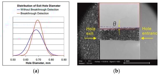
Figure 1.
Real manufacturing film hole data. (a) Hole diameter deviation distribution [3]; (b) conical angle deviations [3].
Some investigators evaluated the effect of film cooling hole geometrical deviations on the heat transfer performance and aerodynamic characteristics. Johnson et al. [9] studied the impact of geometric deviations on the distribution of adiabatic cooling effectiveness values (η) of a row of cylindrical holes using both experimental and CFD methods. These cylindrical holes were manufactured using four different manufacturing techniques. The results indicated that the manufacturing technique can have a noticeable effect, either negatively by the impedance of irregularities or positively by creating a diffusion-shaped “cylindrical” hole. Cerantola and Birk [8] compared a sample laser-drilled hole against cylindrical, nozzled, diffusing, and fileted holes assuming adiabatic walls using the CFD method. The diffusing hole was found to deliver the best film cooling due to the lowest effluent velocity and greatest amount of in-hole turbulent production; while the investigated laser-drilled hole exhibited similar cooling and discharge performance to the simplified nozzled holes. S. Haydt et al. [10] examined the potential impact of the manufacturing defect on the film cooling effectiveness for a well-characterized fan-shaped hole known as the 7-7-7 hole. The meter and diffuser of the holes were manufactured by EDM in two separated steps, which led to an offset between the meter and diffuser. Several types and sizes of the offset were studied, and the offset was generally detrimental to the cooling performance, which indicated that gas turbine manufacturers should try to minimize or eliminate the meter-diffuser offset.
Currently, the application of Uncertainty Quantification (UQ) analysis in gas turbines has been carried out by researchers due to the improvement of CFD capability [11]. UQ research on the CFD methods aims to increase and maintain engine efficiency under variability [12]. The CFD Vision 2030 Study [13] of NASA revealed that UQ will be an important direction of CFD in the future. Montomoli et al. [7] studied the effect of filleted edge variations on the distributions of the η value and the Cd values. Over 10% variations of the η and Cd values were found for the cases with the filleted edge from the cases without the filleted edge. Bunker [2] applied Monte Carlo simulations to consider the effect of geometrical parameter and operational parameter variations on thermal boundary conditions for a typical highly-cooled turbine blade. The results showed that the factors determined by the manufacturing of film holes exerted the most important impact levels on the metal temperature distribution and the aerodynamic performance of the cascade.
To extend our understanding of the influence of micro-manufacturing features on the heat transfer performance and aerodynamic characteristics, the current study investigates the impact of the small manufacturing deviations of a baseline 7-7-7 fan-shaped film hole on the distribution of adiabatic cooling effectiveness (η) values and the value of the discharge coefficient (Cd) using CFD methods. The detailed in-hole flow fields are also analyzed. To quantify the uncertainty of η and Cd values due to the manufacturing uncertainty, an UQ analysis is performed using the Polynomial Chaos Expansion (PCE) model. The statistical characteristics (mean values, Standard deviation (Std) values, and Probability Density Function (PDF) values) of η and Cd are also calculated. All the simulations in this paper used the commercial CFD code Star CCM+ with the realizable two-layer k-ε turbulence model.
2. Computational Setup and Validation
2.1. Geometry Models
Small manufacturing deviations were applied to a baseline fan-shaped hole geometry called the 7-7-7 fan-shaped hole [14,15] to study their effect on film cooling. This 7-7-7 fan-shaped hole was developed by Schroeder and Thole [14,15] as a benchmark shape of a hole. The detailed geometry of the hole is shown in Figure 2. Two different baseline 7-7-7 fan-shaped holes with L/D equal to 3.5 and 6.0 were employed in the current study to evaluate the effect of hole length.
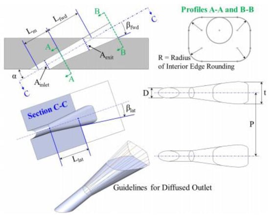
Figure 2.
Shaped hole [14,15].
Three manufacturing deviations of the fan-shaped hole, conical angles (θ), filleted edges (fillet), and diameter deviations (ΔD), as shown in Figure 3, were studied. The hole diameter deviation only occurred in the hole’s cylindrical section, which is always drilled using a low-cost manufacturing process, e.g., laser drilling. The diffuser section of the hole does not always feature this size deviation due to higher precision manufacturing processes.
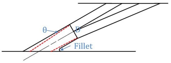
Figure 3.
The three manufacturing deviation factors of the fan-shaped hole conical angles (θ), filleted edges (fillet), and diameter deviations (D).
In order to make a clear distinction for the hole geometric model with the small geometric deviation, 0 shows the schematic of the hole geometry with hole diameter deviations (Figure 4a), conical angle (Figure 4b), and filleted edges (Figure 4c).
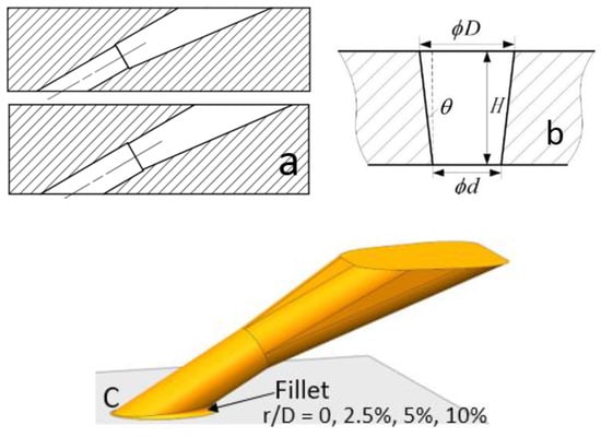
Figure 4.
Schematic of the hole geometry: (a) hole geometry with hole diameter deviations; (b) hole geometry with conical angle; (c) hole geometry with filleted edges.
The hole diameter deviation of the circular hole section resulted in a small step at the interface of the cylindrical and expansion sections. The hole diameter deviation was set to be in the range of ±10% of the diameter of the baseline geometry. The diameter deviation was assumed to be a Gaussian distribution as [2,3]. Five samples were chosen for the CFD simulation and were denoted as the cases D1–D5 (where D1, D2 < mean value of 7.75 mm; D3 is equal to 7.75 mm; and D4, D5 > mean value of 7.75 mm).
The conical angle (Figure 4b) of the fan-shaped hole deviation is defined as [3,5]:
which is determined by the hole diameter deviation along the hole central axis. Based on the maximum hole diameter deviation values, the conical angle of the drilling hole deviation was 0.95°. In the present study, conical angle values of 0°, 0.25°, 0.5°, and 0.8° were selected, and cases with these conical angle values are represented as C1, C2, C3, and C4. The filleted edge (Figure 4c) was chosen as r/D = 0, 2.5%, 5%, and 10% by referring to previous studies [7].
2.2. Numerical Method and Validation
To match the design size of the baseline 7-7-7 fan-shaped film hole, the diameter of the hole (D) was 7.75 mm. The width plenum (pitch-wise size) was 6D. The origin point was the middle of the trailing edge of the hole exit. The mainstream inlet was 10D upstream of the origin, and the mainstream outlet was 30D downstream of the origin. Other cases to be simulated will use the same mainstream domain and the same coolant domain, but different hole shapes.
Polyhedral meshes were generated using STAR-CCM+, as shown in Figure 5. The grid on the bottom wall of the mainstream was refined. Prismatic grids were distributed near all the non-slip walls to make y+ is close to 1. Three-dimensional steady viscous Reynolds-averaged Navier–Stokes equations were solved for the film cooling problems using the commercial CFD code STAR-CCM+.
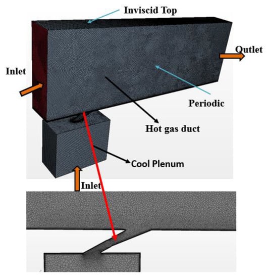
Figure 5.
The schematic of the CFD domain, the polyhedral mesh with prismatic grid near the wall, and the boundary conditions.
The boundary conditions were determined to match an experiment case done by Schroeder et al. [14]. Velocity and total temperature were set at the mainstream inlet. Static pressure was imposed at the outlet. A 10 °C difference in temperature was set between the mainstream and the coolant. The mass flow rate of the coolant was imposed on the coolant inlet to match the blowing ratio (M) as one because the 7-7-7 exhibited the largest film cooling effectiveness values with the blowing ratio equal to 1. All the walls were set as adiabatic. The detailed boundary conditions are listed in Table 1.

Table 1.
Boundary conditions.
To reduce the impact of epistemic uncertainty, numerical validation was performed against the experiment done by Schroeder et al. [14]. Several different turbulence models, such as the standard k-ε model, the realizable k-ε model, the V2F model (The V2f model is based on the standard k-ε model by adding the turbulence anisotropy to the near-wall, it also contains the non-local pressure-strain effects), the EB model, and the RST model, were employed to predict the adiabatic cooling effectiveness distributions and to compare the adiabatic cooling effectiveness distributions with the experimental data. Figure 6 plots the lateral averaged adiabatic cooling effectiveness distributions by experiment and by CFD with the standard k-ε model, the realizable k-ε model, the V2F model, the EB model, and the RST model. Figure 7 shows the adiabatic cooling effectiveness distributions. The lateral averaged η predicted by the standard k-ε model and the realizable k-ε model were in better agreement with the experimental data by Schroeder et al. [14] than those by other turbulence models. Comparing the distribution of the η on the wall between the experimental data and the data predicted by the standard k-ε model and the realizable k-ε model, the realizable k-ε equations modeled the current film cooling problem best; thus, the realizable k-ε model was applied in the CFD simulations in the current study.
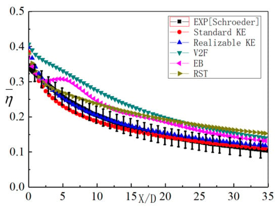
Figure 6.
Lateral averaged adiabatic cooling effectiveness distributions by experiment and by CFD with the standard k-ε model, the realizable k-ε model, the V2F model, the EB model, and the RST model.
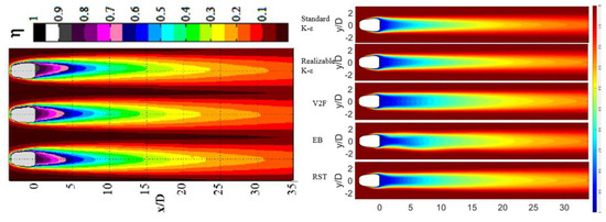
Figure 7.
Adiabatic cooling effectiveness distributions by experiment and by CFD with the standard k-ε model, the realizable k-ε model, the V2F model, the EB model, and the RST model.
Therefore, due to the agreement between the CFD results and the experimental data with the blowing ratio equal to 1 and the density ratio equal to 1.5, the geometric uncertainty analysis was conducted with the same coolant flow condition.
A grid independence test was carried out (see Figure 8) in which lateral averaged film cooling effectiveness distributions in the streamwise direction with 0.2 million, 1.1 million, and 2.5 million grid points were compared with one another and with the experimental data. With the 2.27-times grid refinement (1.1 million–2.5 million), the lateral averaged cooling effectiveness value changes were invisible. The 1.1 million mesh method was therefore employed in this study.
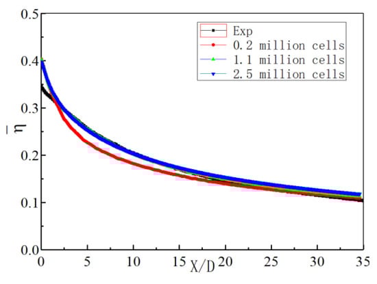
Figure 8.
Grid independency test: lateral averaged film cooling effectiveness with the 0.2 million grid, 1.1 million grid, and 2.5 million grid; M = 1.0 and DR = 1.5.
3. Uncertainty Quantification Methodology
The UQ method used in this study was the non-intrusive Polynomial Chaos Expansion (PCE). This method was first introduced by Wiener [16], using the Hermite orthogonal polynomial to build the PCE model. Xiu and Karniadakis [17] improved it and proposed a generalized polynomial chaos to deal with different distribution forms. This generalized PCE was employed in the current study.
The mathematical basis of the PCE method is polynomial theory, which is equivalent to constructing a surrogate model for random variables, and uncertainty analysis was performed on the surrogate model. Strict mathematical proofs showed that there were corresponding optimal orthogonal polynomial bases for different distribution forms and converging at exponential velocity [11].
The PCE model can be constructed by expanding the random output variable on the orthogonal polynomial basis, as follows:
where θ represents the input random variable and ψ represents the orthogonal polynomial basis.
The above formula can also be abbreviated into a common format:
In the PCE model, there is a relationship between the unknown coefficient and the dimension of the order and random variables.
in which is the dimension of the random variable and is the order of PCE truncating. Once the PCE is built, the unknown coefficients of the PCE model can be solved with projection or projection-regression.
The Stochastic Response Surface Method (SRSM) was used to solve the unknown coefficients in the PCE model [11,18]. The method was proposed by Dr. Isukapalli [19,20]. The coefficient was evaluated from the oversampling point with the least-squares approach [11]. It is generally believed that a sample with twice the number of unknown PCE coefficients can be used to obtain satisfactory results. The use of an oversampling ratio of around 2 could improve the robustness of the method. In addition, this treatment method also prevented some examples from getting a convergent solution.
Bringing the sample and the corresponding function output into the PCE model, you will get the following determinant:
The above formula can be expressed as:
To solve the PCE coefficients with the least-squares approach,
After obtaining the PCE coefficient, the PCE model was built. Then the random output variable could be obtained. One of the methods was analytical. The mean and stand deviation of the random output variable could be calculated by the formula,
Another method using the Monte Carlo (MC) method to solve the mean and stand deviation based on the PCE model was also carried out in the current study. Then, the probability density of the output variable can be obtained.
4. Results and Discussion
4.1. Film Cooling Effectiveness
4.1.1. Effect of the Conical Angle Deviation on Film Cooling Effectiveness
Figure 9 shows the laterally-averaged adiabatic film cooling effectiveness () with the drilled conical angle equal to 0°, 0.25°, 0.5°, and 0.8° adapted from the two baseline 7-7-7 fan-shaped holes with L/D = 3.5 and L/D = 6. The drilled conical angle deviation exerted no evident effect on the value of . This phenomenon was not consistent with that from an investigation with the baseline cylindrical hole geometry by Wen [3]. It was found that the existence of a conical angle may result in negative effects on the aerodynamic and heat transfer performance of the film cooling. However, for the fan-shaped hole in the current study, the impact of the conical angle deviation on the film hole heat transfer performance can be negligible. For the geometry adaption of the conical angle deviations in the current study, only the cylindrical part of the fan-shaped hole as adapted, while the diffuser part of the hole remained unchanged, which made the lateral expansion capacity of the in-hole cool air remain the same, resulting in almost a constant local blowing ratio value and jet momentum value for the holes with conical angle adaption. Therefore, η remained unchanged with conical angle adaption. As a result, the effect of the meter section offset on film holes’ heat transfer performance can be reduced if the manufacturing accuracy of the diffuser section is high. However, the adaption of conical angle deviation on the film hole geometry can be effective on the aerodynamic characteristic, e.g., discharge coefficient (Cd), which will be discussed later in the current paper.
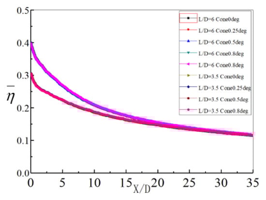
Figure 9.
Laterally-averaged adiabatic film cooling effectiveness () for the drilled conical angle deviations (0°, 0.25°, 0.5°, and 0.8°) for holes with L/D = 3.5 and L/D = 6.
Figure 10 shows the distribution of the η for the two fan-shaped hole case of L/D = 3.5 and L/D = 6 adapted with conical angle equal to 0.8°. The lateral diffusion of the cool air for the case with L/D = 6 was considerably stronger than that of the case with L/D = 3.5, which made the lateral coverage area larger, but the streamwise coverage length shorter for the case with L/D = 6 than that for the case with L/D = 3.5. The reason can be attributed to the difference in the hole exit area. With larger hole length-to-diameter ratio values, the hole exit area will be larger. According to a study by Haydt et al. [21] on the effects of area ratio on the distributions of η for the baseline 7–7–7 fan-shaped hole, η increases with the increase of the ratio of the hole exit area value to hole entrance area value. Therefore, it can be a reason why the hole with L/D = 6 features better cooling performance than that of the hole with L/D = 3.5 even with conical angle adaption.
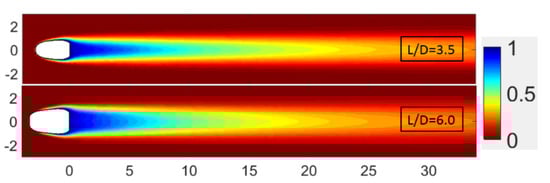
Figure 10.
Distribution of the η for the two fan-shaped hole case of L/D = 3.5 and L/D = 6 adapted with conical angle equal to 0.8°.
4.1.2. Effect of the Diameter and Filleted Edge Deviations on Film Cooling Effectiveness
The filleted edge and diameter deviation are not independent factors for the film cooling effectiveness. The two factors interact with each other.
Figure 11 presents the area averaged adiabatic cooling effectiveness () with diameter deviations of D1, D2, D3, D4, and D5 and with fillet deviations of 0, 2.5%, 5%, and 10%. The area averaged calculation was done through a rectangle of x/D = 0~30 and y/D = −3~3. For all the cases with both diameter deviations and fillet deviations, the value initially decreased and then stabilized when the radius of the filleted edge increased. Therefore, the effect of the fillet adaption on was in a certain range for the current study, and the smaller the fillet, the more evident the change by the filleted edge. For the case with no diameter adaption, the change of value due to the fillet edge can be up to 3.4%, while for the case with the D1 diameter adaption, the change of the value due to the fillet edge can be up to 7.6%.
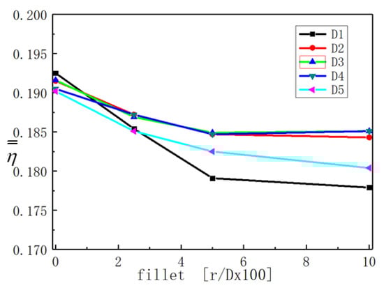
Figure 11.
Area averaged adiabatic cooling effectiveness () with diameter deviations of D1, D2, D3, D4, and D5 and with fillet deviations of 0, 2.5%, 5%, and 10% (averaged through x/D = 0~30, y/D = −3~3).
With the filleted edge radius equal to zero, the influence on the value by the diameter deviation was small. The value decreased with the diameter of the hole increasing. Cases with smaller diameters (D1,D2) than that of the baseline case acquired larger values than that of the baseline case. However, with filleted edges and diameter deviations, all the cases with diameter deviations, no matter positive or negative, featured a decrease in the value from the baseline case. With a larger radius of the filleted edge, the deviations of the value were larger. This makes it important to understand the change in the flow field with the filleted edge adaption. The in-hole flow field with different filleted edge adaptions will be discussed later.
4.2. Discharge Coefficient
4.2.1. Effect of the Conical Angles on the Discharge Coefficient
Figure 12 shows the discharge coefficient values (Cd) for the drilled conical angle deviations (0°, 0.25°, 0.5°, and 0.8°) for holes with L/D = 3.5 and L/D = 6 in the current boundary condition. Cd is a measure of the aerodynamic performance of the film hole, which is defined as:
in which Pm is the mainstream pressure and Ptc is the total pressure of the coolant.
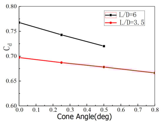
Figure 12.
Discharge coefficient values (Cd) for the drilled conical angle deviations (0°, 0.25°, 0.5°, and 0.8°) for holes with L/D = 3.5 and L/D = 6.
Though the conical angle deviation did not change the value much, it affected the film hole Cd value visibly. With a conical angle, the meter section contracted along the coolant streamline, increasing the blockage effect, thus changing the Cd value. With the conical angle deviation equal to 0.5°, the Cd value was 6.2% less than the baseline case for the case of the hole with L/D = 6. With the angle deviation equal to 1.0°, the change in the Cd value from the baseline case was up to 12.9%. For cases with L/D = 3.5, the Cd value and the change of the Cd value were smaller than those of the case with L/D = 6. It is interesting to note that the Cd value and the conical angle featured a linear relation.
With a smaller Cd value and an unchanged value by conical angle adaption, the coolant supply pressure must be increased to maintain the jet mass flow rate with the conical angle arising in the drilling film hole, or the mass flow rate of the coolant will decrease with supply pressure unchanged. It will change the distribution of pressure or the distribution of coolant mass flow rate in the blade, thus resulting in the imbalance of the surface temperature of the blade. Therefore, the existence of the conical angle should be considered in the initial design phase.
4.2.2. Effect of the Diameter and Filleted Edge Deviations on the Discharge Coefficient
Figure 13 shows discharge coefficient values (Cd) with diameter deviations of D1, D2, D3, D4, and D5 and with fillet deviations of 0, 2.5%, 5%, and 10%. The positive deviation of the diameter increased the Cd value, indicating that the discharge performance of the hole was improved. With larger flow area by the position diameter deviation, the blockage effect of the hole was decreased, and the discharge performance was improved. Thus, with negative diameter deviation, the holes featured smaller Cd values than that of the baseline case.

Figure 13.
Discharge coefficient values (Cd) with diameter deviations of D1, D2, D3, D4, and D5 and with fillet deviations of 0, 2.5%, 5%, and 10%.
With the increase of the radius of the filled edge, the Cd value increased, though the value decreased. For cases with the same diameter deviation values, the Cd value was almost linear to the radius of the filled edge. The widespread existing of the filleted edges in the real blade or in the experimental conditions can be a reason for the underestimation of the Cd value and the overestimation of the value (Adami [22]) calculated by the CFD method compared with the experimental data, as the micro-geometric features and deviations such as fillet and step are often simplified and ignored in numerical simulations.
4.3. In-Hole Flow Field with Filleted Edge
To understand the effect of the filleted edge on the heat transfer performance and discharge performance, the in-hole flow field with filleted edges are studied in the current paper. Figure 14 is the schematic of the in-hole planes (red lines) chosen to plot the velocity distributions, and Figure 15 shows the velocity distributions on the chosen planes for the case without a filleted edge and the case with a filleted edge of r/D = 10%. For the baseline case, the cool air came from the large plenum, and the flow accelerated and deflected into the hole. Thus, a counter rotating kidney vortex (CRVP) formed in the entrance of the hole, resulting in a lower velocity zone near the trailing edge of the hole. With the expansion of the flow passage in the diffuser part of the hole, the high velocity zone near the hole leading edge decelerated along the hole central axis, and the pressure gradients between the leading edge and the trailing edge were smaller in the diffuser part of the hole than that in the cylinder part of the hole, making the CRVP move up to the center of the hole and spread laterally. For the case with the filleted edge, the acceleration of the flow in the hole inlet was more gradual, and the kidney vortex was substantially weaker than the baseline case and attached to the trailing edge of the hole. Due to the small distance of the CRVP for the case with the filleted edge, the flow deflected again in the interface of the meter and diffuser sections because of the backward wall. An Anti-Counter-Rotating Vortex (ACRV) formed there and was reinforced along the streamlines, which can be beneficial to the heat transfer performance, but detrimental to the discharge performance of the hole.
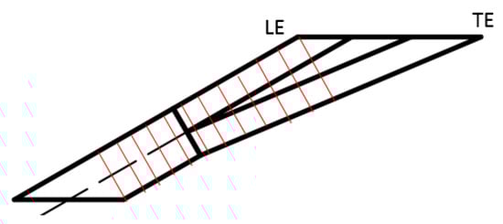
Figure 14.
Schematic of the in-hole planes (red lines) chosen to plot the velocity distributions.
Figure 15.
Velocity contour for different planes in-hole with fillet deviation only: the top is r/D = 0%; the bottom is r/D = 10%.
Figure 16 shows the velocity and vector distributions on the center plane (Y = 0) of the hole with filleted edge radius equal to 0D, 2.5%D, 5%D, and 10%D. There was “jetting region” and “separation region” inside of the holes for the four cases. There were two separation zones inside of the hole. One was due to the jetting effect in the hole inlet. The other large separation zone was in the diffuser part of the hole due to the laying back of the hole trailing edge. At the region near the hole inlet, the coolant was compressed to move near the wall of the leading edge because of the high velocity jetting region with a sharp edge or a small radius filleted edge, making the separation zone delayed in-tube for these cases. However, the low-speed region was thicker for the sharp edge case, making the turbulent mixing effect between the jetting and separation regions stronger; thus, the velocity at the hole exit near the leading edge was smaller than that in the cases with filleted edges. The mixing between the coolant and mainstream hot gas was weaker for the sharp-edge case, improving the coolant coverage. The separation region produced by the diffuser part for the cases with fillet edge was further from the trailing edge and smaller in size, making the high-speed airflow in the jetting region directly spray out of the film hole without sufficient in-hole mixing. The velocity near the leading edge of hole exit for the cases with filleted edge was higher than that of the baseline, exerting a strong reverse impulse on the mainstream. As a result, the coolant coverage for cases with fillet was worse than that for the sharp-edge case.
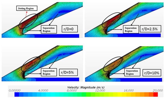
Figure 16.
Velocity distributions and vectors distributions on the Y = 0 plane with the filleted edge radius equal to 0D, 2.5%D, 5%D, and 10%D.
4.4. UQ Analysis
According to the results in Section 4.1, Section 4.2 and Section 4.3, the small geometric deviations by manufacturing process, such as conical angles, filleted edges, and diameter deviations of the hole, can change the heat transfer and aerodynamic performance of the hole visibly, which makes the performance of the film holes uncertain due to random geometry deviations. It is important to quantify this uncertainty based on the random geometry deviations and consider it in the initial design phase.
UQ analysis aims to provide a framework to calculate the effects of the input parameter uncertainty on the model output variables. This analysis is used to determine the effects of the uncertainty factors (manufacturing tolerances or boundary conditions) on the cooling system and reduce the variability in the final design. In the current study, the PCE model of the UQ analysis was constructed based on two factors: the hole diameter and the fillet radii. SRSM was used to solve the PCE model coefficients in this paper.
Figure 17 shows the 95% confidence interval distribution for the lateral averaged adiabatic cooling effectiveness () value and the adiabatic cooling effectiveness (η) value along the centerline. The hole diameter deviation distributed as , and the fillet radii r/D = 0, 2.5%, 5%, and 10%. The range of the 95% confidence interval for the for the value and the η value along the centerline were very small relative to their values, which indicates that the η value is not sensitive to the hole diameter and fillet radii deviations. This is mainly because only the cylindrical part of the fan-shaped hole was adapted, while the diffuser part of the hole remained almost unchanged. As previously mentioned, the fillet radii affected the in-hole flow field greatly, which can have greater influence on the Cd value than that on the η value.
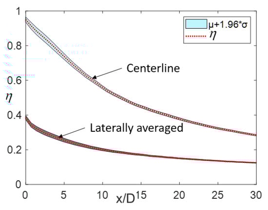
Figure 17.
The 95% confidence interval distribution of the lateral averaged adiabatic cooling effectiveness () value and the adiabatic cooling effectiveness (η) value along the centerline with the hole diameter deviation distributed as and the fillet radii r/D = 0, 2.5%, 5%, 10%.
Figure 18 shows the distributions of the statistical parameters of η: the mean value distribution and the standard deviation value distribution. The distribution of the mean value of η was almost the same as that of the baseline case. However, there were visible deviations of the η distributions. The deviation of η was larger in the near hole region, mainly near the region where the CRVP existed, which indicated that the adaption in the distribution of η was mainly due to the exists of the ACRV and the change in the structures of the CRVP, as previously informed.
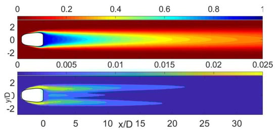
Figure 18.
Distributions of the statistical parameters of η; top: mean value; bottom: standard deviation value.
Figure 19 shows the PDF distribution of the area averaged adiabatic cooling effectiveness () and the value of Cd. The PDF of the value did not fit for the regular Gaussian distribution. It was distributed over a small range with the average value of 0.1854. The unfitting for the standard deviation was because the standard deviation of the statistics was small. This also indicates that the hole diameter and fillet radii deviations had little effect on the value.
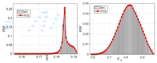
Figure 19.
PDF distribution of the area averaged adiabatic cooling effectiveness () and the value of Cd.
However, the PDF distribution of the Cd value basically still satisfied the Gaussian distribution. As mentioned previously, the variation of hole diameter satisfied the Gaussian distribution, and the fillet radii satisfied the uniform distribution for the PCE model. The Cd value was almost linear to fillet radii (which can be found in Figure 13). The coefficient of variation of Cd was 0.074, which was less than the coefficient of variation of hole diameter. All these factors resulted in the propagation characteristics of the input uncertainty variables.
5. Conclusions
This study investigates the effects of small geometric deviations on the values of η and Cd by using the baseline 7-7-7 fan-shaped hole. A detailed flow field analysis was carried out to determine the impact mechanism of geometric deviation on film cooling. To quantify the uncertainty of η and Cd values due to the manufacturing uncertainty, an UQ analysis was implemented with PCE to obtain the statistical characteristics (the mean value and Std of η and Cd), which were caused by the geometric deviations. The following conclusions were obtained.
- Conical angle deviation exerts no obvious effect on η. However, Cd decreases by 6.2% when the conical angle deviation is 0.5° and increases to 12.9 when the angle is 1.0°.
- The presence of diameter and fillet deviations produces a superposition effect. The area average η decreases by 3.4%, and Cd increases to 15.2% with the fillet deviation existing alone. However, the values are 7.6% and 25.7% when the two deviations exist.
- The decrease in Cd is mainly caused by the weakened streamwise vorticity of in-tube and the blockage effect when the hole possesses a fillet. The velocity distribution of the hole exit exerts an important impact on the change in η.
- The UQ analysis shows that the 95% confidence interval of the centerline and laterally-averaged η both are relatively small. The effects of cylindrical section deviations on η is limited, and the fillet radii mainly affects the flow field in-hole. The result also shows that the PDF of area average η does not satisfy the regular distribution, while the PDF of Cd basically still satisfies the Gaussian distribution.
Author Contributions
Writing, original draft preparation, W.S.; proofread and revise, P.C.; supervision, X.L. and H.J.; funding acquisition, J.R.
Funding
This study is supported by the National Natural Science Foundation of China (Project No. 51676106).
Acknowledgments
The authors appreciate Fenfen Xiong from Beijing Institute of Technology for the guidance on the PCE method.
Conflicts of Interest
The authors declare no conflict of interest.
Nomenclature
| EDM | Electrical Discharge Machining |
| AM | Additive Manufacturing |
| Cd | discharge coefficient |
| UQ | Uncertainty quantification |
| PCE | Polynomial Chaos Expansion |
| Std | Standard deviation |
| Probability Density Function | |
| SRSM | Stochastic Response Surface Method |
| MC | Monte Carlo |
| L | Hole Length |
| D | Hole Diameter |
| TIT | Turbine Inlet Temperature |
| BR | Blowing ratio |
| DR | Density Ratio |
| r | Fillet radius |
| EB | Elliptic Blending model |
| Pm | mainstream pressure |
| Ptc | total pressure of the coolant |
| LE | Leading Edge of hole |
| TE | Trailing Edge of hole |
| CRVP | Counter Rotating Vortex Pair |
| RST | Reynolds Stress Turbulence |
| Greek symbols | |
| Film cooling effectiveness | |
| Conical angle | |
| Subscripts | |
| w | wall |
| mainstream flow | |
| c | inlet of coolant duct |
| aw | adiabatic wall |
| entrance | |
| exit | |
References
- Bunker, R.S. Gas Turbine Cooling: Moving from Macro to Micro Cooling. ASME Conf. Proc. 2013, 2013, 94277. [Google Scholar]
- Bunker, R.S. The Effects of Manufacturing Tolerances on Gas Turbine Cooling. J. Turbomach. 2009, 131, 041018. [Google Scholar] [CrossRef]
- PRIMA North America, Inc. Laser Drilling of Cylindrical and Shaped Holes. Available online: https://slideplayer.com/slide/6880655/ (accessed on 20 September 2017).
- Wen, Z.; Pei, H.; Zhang, C.; Wang, B. Analysis of Surface Quality of Multi-film Cooling Holes in Nickel-based Single Crystal Superalloy. Mater. Sci. Technol. 2016, 32, 1845–1854. [Google Scholar] [CrossRef]
- Maina, M.R. Modeling and Control of Nd: YAG Laser Percussion Drilling of Nickel-Based Super Alloys. Master’s Thesis, Jomo Kenyatta University of Agriculture and Technology, Juja, Kenya, 2015. [Google Scholar]
- Ramesh, S.; Ramirez, D.G.; Ekkad, S.V.; Alvin, M.A. Analysis of film cooling performance of advanced tripod hole geometries with and without manufacturing features. J. Heat Mass Transf. 2016, 94, 9–19. [Google Scholar] [CrossRef]
- Montomoli, F.; Massini, M.; Salvadori, S.; Martelli, F. Geometrical Uncertainty and Film Cooling: Fillet radii. J. Turbomach. 2012, 134, 011019. [Google Scholar] [CrossRef]
- Cerantola, D.J.; Birk, A.M. Quantifying Blowing Ratio for Shaped Cooling Holes. J. Turbomach. 2018, 140, 021008. [Google Scholar] [CrossRef]
- Johnson, P.L.; Ricklick, M.; Kapat, J.S.; Zuniga, H.; Brown, G. The Impact of Manufacturing Techniques on Film Cooling Effectiveness. In Proceedings of the 49th AIAA/ASME/SAE/ASEE Joint Propulsion Conference, San Jose, CA, USA, 15–17 July 2013. [Google Scholar]
- Haydt, S.; Lynch, S.; Lewis, S. The Effect of a Meter-Diffuser Offset on Shaped Film Cooling Hole Adiabatic Effectiveness. J. Turbomach. 2017, 139, 091012. [Google Scholar] [CrossRef]
- Montomoli, F.; Carnevale, M.; D’Ammaro, A.; Massini, M.; Salvadori, S. Uncertainty Quantification in Computational Fluid Dynamics and Aircraft Engines, 2nd ed.; Springer: Cham, Switzerland, 2018. [Google Scholar]
- Seshadri, P.; Shahpar, S.; Parks, G. Aggressive Design in Turbomachinery. In Proceedings of the 7th Dresdner Probabilistic Workshop, Dresden, Germany, 9 October 2014. [Google Scholar]
- Slotnick, J.; Khodadoust, A.; Alonso, J.; Darmofal, D.; Gropp, W.; Lurie, E.; Mavriplis, D. CFD Vision 2030 Study: A Path to Revolutionary Computational Aerosciences; NASA/CR-2014-218178; NASA Langley Research Center: Hampton, VA, USA, 2014.
- Schroeder, R.P.; Thole, K.A. Adiabatic Effectiveness Measurements for a Baseline Shaped Film Cooling Hole. In Proceedings of the ASME Turbo Expo 2014: Turbine Turbine Technical Conference and Exposition, Düsseldorf, Germany, 16–20 July 2014. GT2014-25992. [Google Scholar]
- Schroeder, R.P.; Thole, K.A. Effect of high freestream turbulence on flowfields of shaped film cooling holes. J. Turbomach. 2016, 138, 091001. [Google Scholar] [CrossRef]
- Wiener, N. The homogeneous chaos. Am. J. Math. 1938, 60, 897–936. [Google Scholar] [CrossRef]
- Xiu, D.; Karniadakis, G.E. The Wiener—Askey polynomial chaos for stochastic differential equations. SIAM J. Sci. Comput. 2002, 24, 619–644. [Google Scholar] [CrossRef]
- Xiong, F.; Yang, S. Engineering Probability Uncertainty Analysis Method; Science Press: Beijing, China, 2015. [Google Scholar]
- Isukapalli, S.S. Uncertainty Analysis of Transport-Transformation Models. Ph.D. Thesis, The State University of New Jersey, New Brunswick, NJ, USA, 1999. [Google Scholar]
- Isukapalli, S.S.; Roy, A.; Georgopoulos, P.G. Efficient sensitivity/uncertainty analysis using the combined stochastic response surface method and automated differentiation: Application to environmental and biological systems. Risk Anal. 2000, 20, 591–602. [Google Scholar] [CrossRef] [PubMed]
- Haydt, S.; Lynch, S.; Lewis, S. The Effect of Area Ratio Change via Increased Hole Length for Shaped Film Cooling Holes With Constant Expansion Angles. J. Turbomach. 2018, 140, 051002. [Google Scholar] [CrossRef]
- Adami, P.; Martelli, F.; Montomoli, F.; Saumweber, C. Numerical Investigation of Internal Crossflow Film Cooling. In Proceedings of the ASME Turbo Expo 2002: Power for Land, Sea, and Air, Amsterdam, The Netherlands, 3–6 June 2002; pp. 51–63. [Google Scholar]
© 2019 by the authors. Licensee MDPI, Basel, Switzerland. This article is an open access article distributed under the terms and conditions of the Creative Commons Attribution (CC BY) license (http://creativecommons.org/licenses/by/4.0/).