Article

The Interactive Design Approach for Aerodynamic Shape Design Optimisation of the Aegis UAV

School of Aerospace, Transport and Manufacturing, Cranfield University, MK43 0AL, UK
*
Author to whom correspondence should be addressed.
Aerospace 2019, 6(4), 42; https://doi.org/10.3390/aerospace6040042
Submission received: 27 February 2019 / Revised: 1 April 2019 / Accepted: 4 April 2019 / Published: 8 April 2019
(This article belongs to the Special Issue Multidisciplinary Design Optimization in Aerospace Engineering)

Abstract

:
In this work, an interactive optimisation framework—a combination of a low fidelity flow solver, Athena Vortex Lattice (AVL), and an interactive Multi-Objective Particle Swarm Optimisation (MOPSO)—is proposed for aerodynamic shape design optimisation of any aerial vehicle platform. This paper demonstrates the benefits of interactive optimisation—reduction of computational time with high optimality levels. Progress towards the most preferred solutions is made by having the Decision Maker (DM) periodically provide preference information once the MOPSO iterations are underway. By involving the DM within the optimisation process, the search is directed to the region of interest, which accelerates the process. The flexibility and efficiency of undertaking optimisation interactively have been demonstrated by comparing the interactive results with the non-interactive results of an optimum design case obtained using Multi-Objective Tabu Search (MOTS) for the Aegis UAV. The obtained results show the superiority of using an interactive approach for the aerodynamic shape design, compared to posteriori approaches. By carrying out the optimisation using interactive MOPSO it was shown to be possible to obtain similar results to non-interactive MOTS with only half the evaluations. Moreover, much of the usual complexity of post-data-analysis with posteriori approaches is avoided, since the DM is involved in the search process.

Graphical Abstract

1. Introduction

The use of computational optimisation techniques in aerodynamic shape design processes has become conventional because with these techniques the design and development of a complex vehicle is more flexible, quicker, and easier to understand [1]. These techniques have the potential to improve the efficiency of the design process and the quality of the final design. In addition, the rapid growth in computing technology offers design engineers the opportunity to use optimisation in design of real-world applications [2]. Thus, optimisation is now a key technology in the development of innovative real-world applications. However, increasing model complexity and the limitations of even supercomputers makes it challenging to find solutions in an acceptable computation time; computations could take weeks or months to produce a solution that may not even be feasible [3,4]. This poses a serious problem within multi-objective, multi-discipline, optimisation problems, where a number of conflicting objectives must be optimised simultaneously to obtain highly optimal solutions [1,5]. In such optimisation techniques, the whole design space is explored, since no preference is provided by the Decision Maker (DM) to steer the search to the Region of Interest (ROI) once the optimisation process has been started [6,7]. In the software simulations used, this technique requires a large population size to explore the whole design space evenly [8].
However, the DM in most practical applications is interested only in a part of the Pareto front, the specific subset of good solutions. To come up with such results in a suitably short time, the DM must be part of the optimisation process rather than waiting until the process finishes. The main idea is to focus only on the ROI rather than exploring all the design space [9,10], because the benefits from trade-off solutions that lie outside the ROI are very small compared with the computational cost and the efforts required of the DM in analysing unnecessary information [11]. Involving the DM within the optimisation process periodically to provide significant information usually helps with focusing on a sub-part of the design space (see Figure 1). Consequently, computational time is reduced and an optimal solution that satisfies the DM’s preferences is more readily achieved [12,13]. In such an approach, the DM will provide its preference while the iteration is underway. This makes it possible to focus all the computation efforts on exploring only the areas of interest within the search space to identify just the preferred designs for the intended applications.
The aerodynamic design of aircraft has benefited exceptionally from the development of optimisation techniques [14], which have been integrated into the flow solvers’ software to accelerate the process of trade-off between the requirements of different disciplines [15,16]. Conventional optimisation techniques have been explored extensively to help reduce the length of the design cycle [3,17,18,19], motivated by the need to reduce the computational cost of new designs with high optimality solutions [20]. In a multi-objective optimisation problem, the target is usually to find a well-distributed Pareto front instead of a set of solutions that satisfy the DM’s requirements [21,22]. This presents many problems concerning computational cost and data analysis, since once the optimisation process is started, it is not possible for external interaction to guide the search to the ROI. However, by including human input into the optimisation process, the length of the optimisation cycle may be reduced significantly.
Over the last three decades, many researchers have focused on developing interactive multi-objective optimisation methods. The majority of these methods are based on Multi-Attribute Value Theory (MAVT) [6,23], where the performance is captured by asking the DM to compare the non-dominated solutions, either in pairs, or in groups, to formulate the required preference. Based on the DM’s preference, the optimisation problem will be formulated to find a suitable value for the objective function, satisfying the requirement of the DM [6]. The majority of these approaches are based on an Evolutionary Algorithm (EA). For example, in Deb et al.’s study, a methodology is developed to lead the DM to regions of interest depending on its preference, as obtained by using an evolutionary multi-objective optimisation algorithm [8]. Interaction with the DM helps progress towards the preferred solution after a specific number of iterations. The preference is used to model a value function, which is then used until the next interaction.
Ke Li et al. [12] derived an approximation value function to model the DM preference by scoring candidate solutions and then employing an Evolutionary Multi-objective Optimisation (EMO) algorithm to lead the DM to the ROI of its choice. An interesting work by Muberra et al. developed an interactive evolutionary algorithm for multi-objective feature selection depending on the preference-based approach [24]. The DM guides the search to the regions that contain interesting solutions. A supervised learning algorithm is used to assist with measuring the feature selection performance classification, eliminating irrelevant information, improving the time efficiency, and simplifying the optimisation search as a whole. More such evolutionary algorithms can be seen in other studies [8,25,26,27].
In contrast, there are not many studies that use Particle Swarm Optimisation (PSO) for interactive optimisation [13], even though PSO is a comparatively simple concept and is computationally faster and relatively inexpensive in terms of computer memory requirements compared with other population techniques [13,28,29]. Agrawal et al. proposed an interactive particle swarm approach for solving multi-objective optimisation problems, including a DM preference [24]. The interactivity commences only after a finitely large archive of non-dominated solutions is reached. The role of the DM is to select a preferred solution among the non-dominated Pareto solutions by making a pairwise comparison. The approach used an adaptive-grid mechanism for incubation of the particle swarm for the multi-objective optimisation. A good summary of interactive Multi-objective Optimisation Methods based on MAVT can be found in a previous study [8]. However, such methods are not yet applicable to real-world problems. Methods in this category are limited to showing information or plots for selected points in the objective space, whereas the concept of interactive optimisation is to provide enough information about the design space to the DM to be able to steer the optimisation search to the ROI efficiently [30].
The first interactive optimisation approaches based on a non-MAVT-base were presented in a previous study [13]. It used a Multi-Objective Particle Swarm Optimisation (MOPSO) algorithm to guide the particles to the ROI using DM preference by means of a heat-map-visualisation-based user interface. In this method, the DM is not required to review every individual solution to make a choice; it was necessary to focus only on small particles of interest to guide the solutions. Even though this method allowed the DM to focus only on the ROI, it required a large number of interactions [30]. A newer version of the interactive MOPSO using DM interaction was developed in a previous study [6]. It uses the idea of a visualisation-based user interface that implements the Parallel Coordinates technique, and a 2D scatter graph to articulate the DM’s preferences. The approach was used successfully on a 2D aerofoil benchmark problem used by Kipouros et al. in a previous study [31].
The published literature on using an interactive approach for aerodynamic shape optimisation is quite modest. To date, most available papers reporting the use of the interactive technique relate either to standard test problems [7,13,25] or optimisation of a wing airfoil [6]. This work introduces a preference-based framework, which incorporates the flow solver, Athena Vortex Lattice (AVL) [32] with stochastic MOPSO [6], to lead a DM to the solution of its choice using a visualisation-based user interface. The process includes simultaneous optimisation of wing and tail design variables at level flight. To demonstrate the effectiveness and superiority of this approach, we compared the interactive optimisation results obtained using I-MOPSO with the non-interactive results of an optimum design case obtained using the Multi-Objective Tabu Search (MOTS) algorithm [33,34] for the Aegis Unmanned Aerial Vehicle (UAV). The Tabu Search (TS) algorithm is considered as one of the most efficient heuristic methods in the sense of its ability to find a good quality solution in an appropriate computational time [34,35]. Use of MOTS has rapidly expanded in recent years as one of the efficient meta-heuristic techniques dealing with complex real-world problems [36]. Ghisu et al. have argued that researchers previously paid little attention towards the TS algorithm compared to other multi-objective meta-heuristics, but recently TS has gained attention for its use in aerodynamic shape design problems [37].
The results obtained confirmed the ability of the DM to use its preferences effectively to steer the search to the ROI without degrading the aerodynamic performance of the optimised configurations. Even using only half the evaluations, the DM was able to obtain results similar to, or better than, those obtained by the non-interactive use of MOTS and MOPSO. This study demonstrates the great potential of carrying out optimisation interactively at different design phases of any aircraft of any size.
The remainder of this paper is structured as follows. In Section 2, the methodology framework and particle selection scheme used to guide the interactive optimisation search is explained. Design optimisation and architecture of the design problem are described in Section 3. In Section 4, the non-interactive optimisation problem is formulated. The results and discussion for the non-interactive and interactive optimisation are presented in Section 5. Finally, conclusions are given in Section 6.

2. Materials and Methods

The aim of this section is to demonstrate the possibility of using the interactive optimisation approach to accelerate the optimisation of the design process, while retaining all the useful information in the design space. A demonstration of the applicability of the interactive approach is presented through the Aegis UAV design case.
Since most decisions of a DM in practical applications concern regions of the Pareto front, an interactive optimisation framework was proposed, where the DM was involved with the optimisation process in real time, focusing on improving the efficiency of the solutions in terms of computational cost and optimality. In this experiment, a Desktop computer with an i7-6700 CPU processor was used to install the interactive framework.
Before this, significant work was performed by automating the optimisation of the design process and greatly increasing computing power by getting access to the Cluster/Grid [38] using the Nimrod/O tool [39,40,41], as described in a previous study [42]. This enabled the designer to manipulate various combinations of the design variables and better understand different design scenarios that could be used in the initial design phase of the aerodynamic shape design problem. Once the problem was understood better, an interactive optimisation was performed on a selected design scenario focused on accelerating the optimisation process while achieving better solutions.
Details of the structure of each strategy, linking the codes and flow of the data, are explained below.

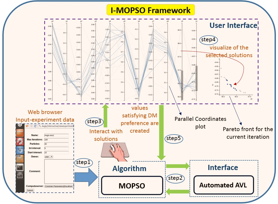
2.1. Interactive Optimisatin Framwork

Figure 2 presents the main components of the interactive optimisation framework used in this work. The primary goal was to accelerate the optimisation search, and to achieve the best optimality level by involving the DM in the overall optimisation process. The decision support framework consists of four main parts; the web browser input data, the main programme (developed in Python), Interface-AVL, and the interactive user interface.
The user-input interface is used to input parameters required for performing interactive optimisation. It is accessible from a common web browser, which is driven by a Python-based web application. This window allows the user to input the number of iterations, number of particles, and the required interactive intervals. The underlying algorithm used in this work was developed and tested by Hettenhausen et al. [6], which was a development of previous work [13], where the user interaction was based on heatmap visualisation. The framework used a posterior optimisation approach with MOPSO [43] as the method for searching and exploring the design space to obtain a set of optimal solutions.
The flow solver used for modelling and simulation of the new UAV configurations is the Athena Vortex Lattice (AVL) [32,44]. This is a low fidelity flow solver using an extended Vortex Lattice Method for generating wings and tails shapes and using slender-body theory for fuselage and nacelle modelling [44]. However, for the automatic reading and filing of this data into new files, an Interface-AVL code was developed [42]. The Interface-AVL is developed to (i) generate the configuration needed to run AVL, (ii) satisfy certain constraints that are required to complete the flight mission, and (iii) compute other quantities that are required to perform the sweep and evaluate the objective function, such as parasite drag [45] and mass properties. The parasite drag was calculated using empirical formulae called build-up techniques, since AVL code is only capable of evaluating inviscid drag [46].
To integrate the external model (Interface-AVL) with the I-MOPSO framework, the framework was amended following Tilocca [47]. Once the optimisation run was started, the DM interacted with the process periodically. The visualisation-based user interface in this framework used a Parallel Coordinates technique [48,49,50] to articulate the DM’s preferences, and provide a 2D scatter graph. Both visualisation tools enabled the DM to make the best decision by recognising the existing trend and correlations between design variables, as well as objective functions [6]. By interacting with the parallel coordinates and 2D scatter graph, it was possible to steer the optimisation search, according to the DM’s expertise and preferences, to focus on the most interesting set of solutions, or even a single solution.

2.1.1. Multi-Objective Particle Swarm Optimisation (MOPSO)

Particle Swarm Optimisation (PSO) is a stochastic population-based algorithm introduced in 1995 by Kennedy and Eberhart [51]. It was inspired by the collaborative behaviour of schools of fish or flocks of birds [29,43,52]. The PSO, initially implemented for neural network training by his authors [51], has now become a very popular global optimiser. Since the PSO is based on a simple concept and is both fast and computationally inexpensive, regarding memory requirements compared to other population techniques, many researchers have extended the algorithm to handle multi-objective optimisation problems [28,29].
The MOPSO algorithm used in this framework was initially developed by Coello Coello and Lechuga [43], then further developed and tested by Hettenhausen et al. [6]. The majority of MOPSO algorithms share the same basic approach—a swarm of a certain number is initialised randomly, and that number will remain constant until the end of the run. The swarm behaviour is bounded by the velocity equation, which is updated continuously and is dependent on both the previous weighted velocity and known good solutions, p p b e s t   and   p g b e s t , representing the individual best particle and the whole swarm, respectively [6].
The velocity equation represents the information exchanged between the particles in the swarm, and it is responsible for updating the position of the particles at each iteration, t + 1 , and can be stated as:
v t + 1 = w v i + c 1 r r ( p p b e s t x t ) + c 2 r 2 ( p g b e s t x t )
where the x t denotes the position of a particle p i in iteration   t , and it is updated using the equation:
x t + 1 ( t ) = x t + v t + 1
where c 1   and   c 2 are positive constants representing the attraction of the particle towards its own success and towards the global best, respectively; r r   and   r 2 , are uniform random weights in the range [ 0 , 1 ] , and w is the inertial weight, which takes a value of 0.4 and is used to control or define the impact of the previous particle velocity on the current particle velocity [43]. Commonly, p p b e s t   and   p g b e s t represent the archive of non-dominating solutions discovered by a specific particle during the iterations and by the whole swarm, respectively.
In order to select a leader, the search space is divided into a hypercube grid (10 × 10). The non-dominated particles are stored in the archive at each iteration and each is defined according to its objective function value. The hypercube grid containing more than one particle will be assigned a fitness equal to the number of particles divided by ten to reduce the fitness of that hypercube. Next, the leader will be selected by applying roulette-wheel selection. This process will continue until the end of the iterations [6,29].
The major difference between the algorithm presented in a previous study [43] and the one used here is the addition of further guidance to p p b e s t and p g b e s t . This is actioned by the DM and executed via “virtual guide particles”. The “virtual guide particles” enhance exploration and diversity in regions and intervals selected by the DM. The DM chooses the ranges of parameters toward which it wishes to guide the optimisation, leaving MOPSO to guide the particle in the direction of the specific interval. Values that satisfy the DM constraint are generated and listed for every dimension in the domain; these originate from identified solutions in the archive and are used to generate the “virtual guide particles”, in accordance with the following conditions.
  • When at most one point satisfying the constraints is found, a random particle is generated via a Gaussian distribution which is centred at the mid-point of the upper and lower boundaries with a standard deviation of about 10% of the separation between the upper and lower boundaries.
  • When more than one point satisfying the constraints is found, but no other boundary limits have been set by the DM, a single value is chosen at random and a small turbulence value is applied to it.
  • When more than one point satisfying the constraints is found and a specific boundary limit has been defined by the user, the value of the parameter is selected as determined by the convergence of the range:
    If the selected range has less than 80% coverage by established points, a single point is randomly selected from within the largest gap.
    If the selected range has more than 80% coverage by established points, an existing point is randomly chosen from within the range, and a small turbulence value applied to it.

2.1.2. Particles Selection Schema on I-MOPSO Interface

The user interface is focused on anticipating what the DM might need to do. It ensures an interface that is easy to access, understand, and use to facilitate the necessary actions. Steering the optimisation process towards the desired solution starts once the DM submits the number of iterations, number of particles, and the interactivity interval. Once the pre-set interval is reached, the DM can start to interact with the optimisation process. In the user interface, each parallel coordinate axis enables the DM to select a range for the designated design variable and objective functions that are assigned to that axis. This is performed by scrolling a grey bar along the desired range within the axis (see Figure 3).
Applying such constraints to multiple axes enables the DM to visualise the correlation that exists between the design variables and objective functions. By selecting a range of the desired solution along the objective axis, particles that contribute to this solution from all the design variables will be highlighted. The analysis and investigation of the highlighted and non-highlighted solutions provides an insight into the correlations that exist between the design variables and objective functions. We would like to stress here that MOPSO in this framework is generating the design variables in the interval [−1, 1]. Thus, the design variables’ values displayed on the parallel coordinates will also be in the interval [−1, 1]. However, scale and translation factors are applied to each design variable after initialisation to deliver those particles with the appropriate values to the external model (Interface-AVL) [47]. Figure 3 shows an example of DM selections that can be made with parallel coordinates, and the corresponding observations that may be obtained from it, as a location on the Pareto front. Note that the DM can select a single particle, which is shown by the colour green on the parallel coordinates and red on the scatter plot.
Experience of the above process has shown that the DM is able to interact with the optimisation process and guide the search in the desired direction. Furthermore, the location of the potential solutions within the Pareto front scatter graph provides a clear idea of the direction in which the solutions must be steered. The scatter graph is used to display the correlation existing between any two parameters in the design space. More details about using the “virtual guide particle” schema to promote those regions considered desirable by the DM can be found in a previous study [13].

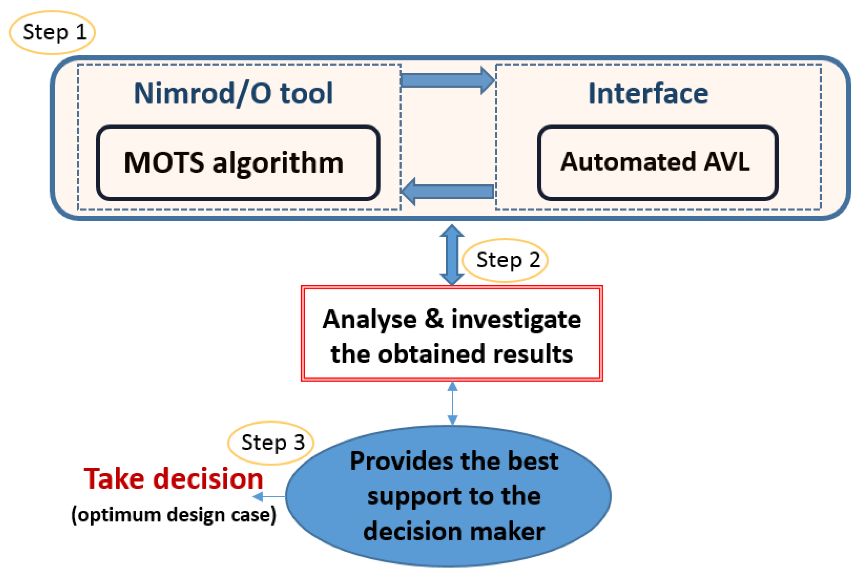
2.2. Automated Optimisation Framework (Non-Interactive)

Figure 4 summarises the components of the automated framework used in the various stages of development. It consists of three main parts: Nimrod/O design optimiser tool, optimiser algorithm (MOTS) [34,35,53], and flow solver. The flow solver used here is the AVL. Due to the fluid nature of the initial design process, it is not recommended to use high fidelity analysis design tools, such as Computational Fluid Dynamics (CFD), at this stage as they can be unnecessarily costly [4,54]. What is required is a tool that strikes a balance between sufficient accuracy and computational cost [55,56,57,58]. Piperni et al. [59] and Zhang et al. [60] have argued that the level of fidelity that should be delivered by the models is mostly determined at the development stage, which the design process aims to enhance. On the other side, the optimisation was performed using the Multi-Objective Tabu Search (MOTS) algorithm, chosen for its suitability for this type of complex aerodynamic design problem [35,36,37].
To define the new geometry for each candidate solution automatically, a code (Interface-AVL) to control the interaction was developed, as described in Section 2.1. The optimisation process required a repetitive evaluation of the objective functions for each candidate, which made the flow solver the most computationally expensive component within the optimisation framework. Thus, if the flow solver is not accurate enough and not able to capture the physical processes of this stage, the optimisation process will converge to solutions that violate the flow characteristics or display numerical errors. The quality of panel discretisation for the lifting surfaces required by the AVL input files were improved using the Sweep Method (SM) [61,62], as in previous work by the authors [42]. The reader may wish to refer to Appendix A for more details on the AVL geometry input file.
The Nimrod/O tool offers a declarative file to allow users to focus on the technical issues of the design problem instead of concerning themselves with programming details. Figure 5 shows an example of a Nimrod/O declarative file, which can be written by any editor. It consists of three main sections; each section defines a particular part of the optimisation process. The first part defines the design variables: integer, float, and text. The second section defines tasks required to be executed. The final section of the schedule file contains the optimisation method. In addition, the schedule file may include constraints, which are located after the first part. The constraints can be either hard or soft—hard cannot be violated, whereas soft can. In the case of soft constraints, penalty values should be added to the objective functions. More sections may appear in the schedule file for the named results. If such sections exist, they will be after the constraints section and linked to the multi-objective optimisation algorithms only. Such sections will specify the number of objective values that will be computed during the run. If such sections are missing, then the value of the objective function is unity. By using this file, the user can simply define the design variable characteristics, tasks to be executed, and the algorithm to be used. Using such a tool, the designer was enabled to execute a computational model over various design variables utilising the resources on a global computational grid. The tool computed the value of the objective function corresponding to different combinations of parameters, and the results were sent to a cluster of processors [31,39,63]. The design space was explored exhaustively over a range of pre-set design variables to minimise a selected objective function (endurance ratio and UAV total mass).
The optimisation started by finding the optimal number of regions and evaluations that were used mainly to define the efficiency of the MOTS algorithm. Once the number for the regions and evaluations was selected, the optimisation process started by performing various design scenarios to explore the UAV characteristics and provide the correct support for the DM to take the best decision (see Section 5.1).

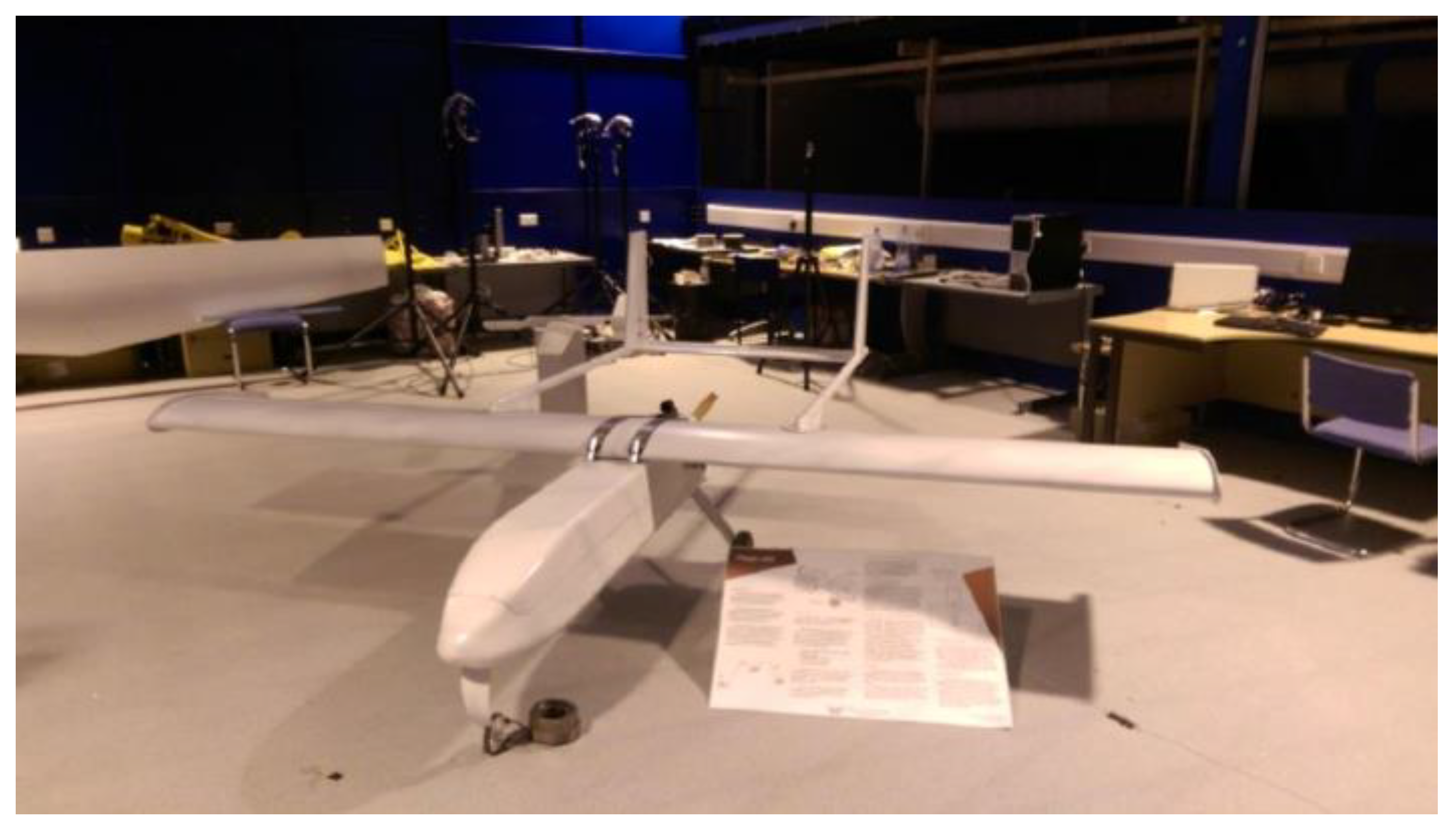
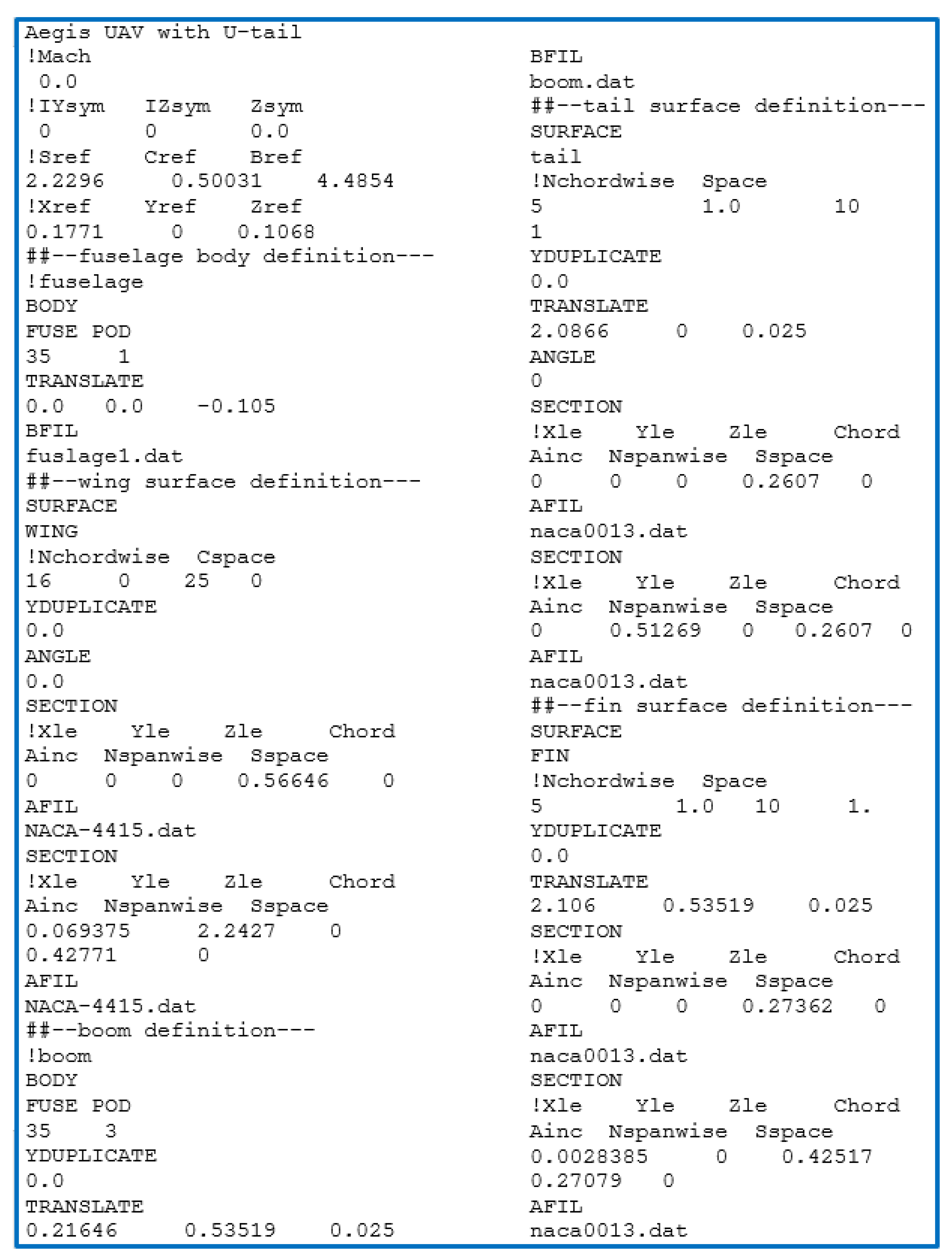
3. Description of Design Optimisation Case Study—Aegis UAV

The design test case used to demonstrate the effectiveness of using optimisations interactively within the proposed framework is the Aegis UAV. It is a project launched by Cranfield University four years ago to develop a medium altitude and long endurance UAV for surveillance missions, and an initial base design configuration was built [64,65]. The design is not yet fully optimised, and there is room for further improvement, and this will be done using optimisation techniques. This project is an integral part of that development.
Figure 6 shows a photograph of the actual model of the Aegis UAV with U-tail configuration. It is designed based upon the AAI RQ-2 Pioneer aircraft used by the USA and Israeli forces. The Aegis UAV has a twin boom pusher configuration, where the tail is mounted on two booms that extend from the wings upper surface. The aircraft utilises rectangular wings, with one of two different tail configurations: U-tail or inverted V-tail. NACA 4415 and NACA 0013 airfoil sections were used for the wing and tail lifting surfaces, respectively. The Aegis UAV with U-tail configuration has a maximum take-off mass of 66 kg, while the Aegis UAV has a weight of 64.5 kg with an inverted V-tail configuration. Both configurations are capable of carrying a 10 to 15 kg payload.
The operational altitude for the UAV is around 2000 m, while the Reynolds number is around 1.5 × 10⁶ based on the chord, and the Mach number is around 0.13. Using AVL, the lift coefficient ( C L ) for level flight was found to be 0.3044 ( C L   = 0 = 0.3044 ) at a cruise speed of 43.60 m/s for the Aegis UAV with U-tail, and 0.3047 ( C L   = 0 = 0.3047 ) at a cruise speed of 43.07 m/s for Aegis UAV with inverted V-tail.

The Architecture of the Design Problem

In a previous study [42], the authors commenced this work with the development of a non-interactive framework that combined the Nimrod/O tool with the flow solver, Athena Vortex Lattice (AVL), to enhance the aerodynamic optimisation process of any aerial vehicle platform. The Aegis UAV has been used to demonstrate the efficiency and reliability of the proposed framework at the conceptual and preliminary design phases. This framework showed efficient exploration of the design space and has established the existing relations between the objectives and the design variables using the Sweep Method (SM) [61,62]. The study and analysis of the results, with the help of visualisation techniques, were used effectively to eliminate any dysfunctions which existed in the developed framework. Then, the SM results were successfully used as feedback to redefine the constraints and re-formulate the design problem.
Two different objectives were included: maximising the endurance ratio ( C L 1.5 / C D ) , and minimising the structural mass ( UAV   mass ) . However, since all the solvers attempt to minimise the objective functions, the endurance ratio ( E ) was redefined as ( C L 1.5 / C D ) . Ideally, the endurance ratio will be an optimum, i.e., by maximising the term ( C L 1.5 / C D ) , using suitable flight conditions and configurations [66,67,68]. This is a single-point optimisation under nominal flight conditions, where the optimiser is seeking to minimise the drag coefficient ( C D ) by varying the shape design variables subject to C L = C L . The C L is the base design lift coefficient.
On the other hand, the total mass of the UAV was the sum of the masses of all the subsystems, including the frame structure, propulsion system, and payloads, and was parameterised in terms of aircraft wing, boom, and tail design variables.
In this study of the design of the Aegis UAV, the following sections will demonstrate the effectiveness of undertaking optimisation interactively through comparisons of results obtained using interactive MOPSO and results obtained using non-interactive MOTS and MOPSO.

4. Formulation of the Non-Interactive Optimisation Problem

Details of two main procedures used to optimise the Aegis UAV configurations used in this research paper, U and inverted V-tail shapes, first used only wing design variables, and then wing-tail design variables simultaneously. Initially four design cases were analysed to demonstrate the effectiveness of the non-interactive framework [42] and gain a better understanding of the design requirements for the Aegis UAV. Table 1 shows the design variables and their upper and lower bounds.

4.1. Using Wing Design Variables

In this case, only wing planform parameters were used to obtain a set of optimal wing configurations for the Aegis UAV with both U-tail and inverted V-tail for steady flight. The optimisation included the following design variables: wing span ( b w ), wing root chord ( C r _ w ), wing taper ratio ( λ w ). The formulation of the design problem was:
min .   f ( x ) =   min { C L 1.5 C D UAV   mass } ,
subject   to :   C L = C L  
  V st ( x )     V st   0
Cm ( x ) Cm
V max ( x ) +   V max   0
x l   x   x u
  x = [ b w   C r _ w   λ w ] T
Here, f ( x ) is the scalar objective function, x is a vector of n components, x l and x u are the lower and upper bounds on each of the design variables, respectively, V st and V max are the optimised UAV stall and maximum velocity, respectively, V st and V max are the base design stall and maximum velocity, respectively, and Cm is the pitching moment coefficient. The design variables were subject to the base design pitching moment ( Cm ) .

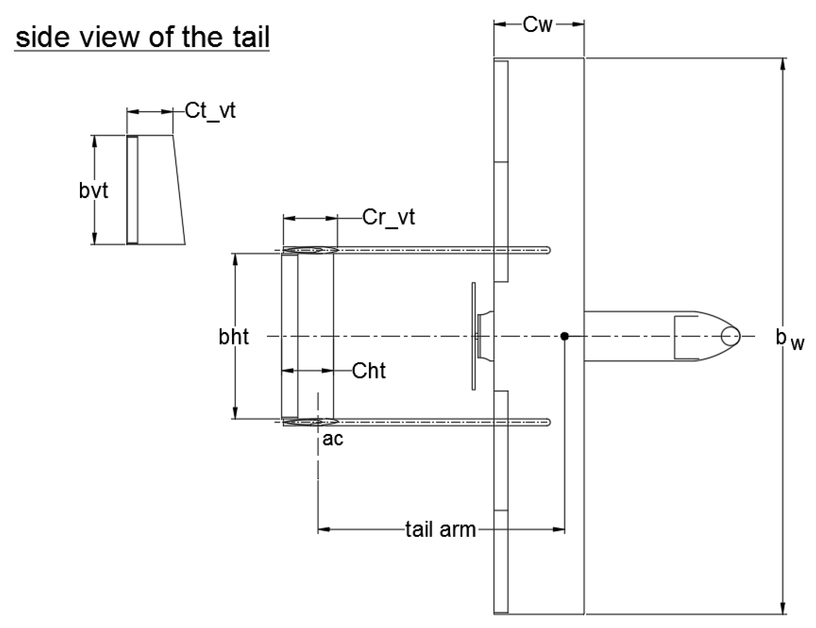
4.2. Using Wing and Tail Design Variables for Aegis UAV with U-tail Shape

In order to obtain a feasible solution for the full UAV configuration by the aerodynamic shape optimisation process, the optimisation problem should include wing and tail design variables simultaneously, since aerodynamic efficiency and stability characteristics are inter-related [66,69,70]. The trade-off in any wing-tail design is between producing the desired stability and control moments versus weight and parasitic drag. Nine design variables are used to optimise the Aegis UAV with U-tail shape: wing span ( b w ), wing root ( C r _ w ), wing taper ratio ( λ w ), horizontal tail volume ( V ht ), vertical tail volume ( V vt ), tail arm ( L t ), horizontal tail aspect ratio ( AR ht ), vertical tail aspect ratio ( AR vt ), and vertical tail taper ratio ( λ vt ) (see Figure 7).
The formulation of the design problem was as follows:
min .   f ( x ) =   min { C L 1.5 C D UAV   mass } ,
subject   to :   C L = C L
Cm ( x ) Cm
  V st ( x )     V st   0
V max ( x ) +   V max   0
bht 1.0   ( geometric   constraint )
Ct _ vt 0.24   ( geometric   constraint )
Cm α 0 ,   Cn b 0 ,   Cl b 0 ,   Cm q 0 ,   Cn r 0
x l   x   x u
x = [ b w   C r _ w   λ w   V ht   V vt   L t   AR ht   AR vt   λ vt ] T
where bht is the horizontal tail span, Ct _ vt is the vertical tail tip, Cm α is a pitching moment slip, Cl b and Cn b are the variation of rolling and yawing force coefficient with sideslip angle, respectively, Cm q is variation of pitching moment coefficient with pitch rate, and Cn r is the variation of yawing force coefficient with yaw rate.

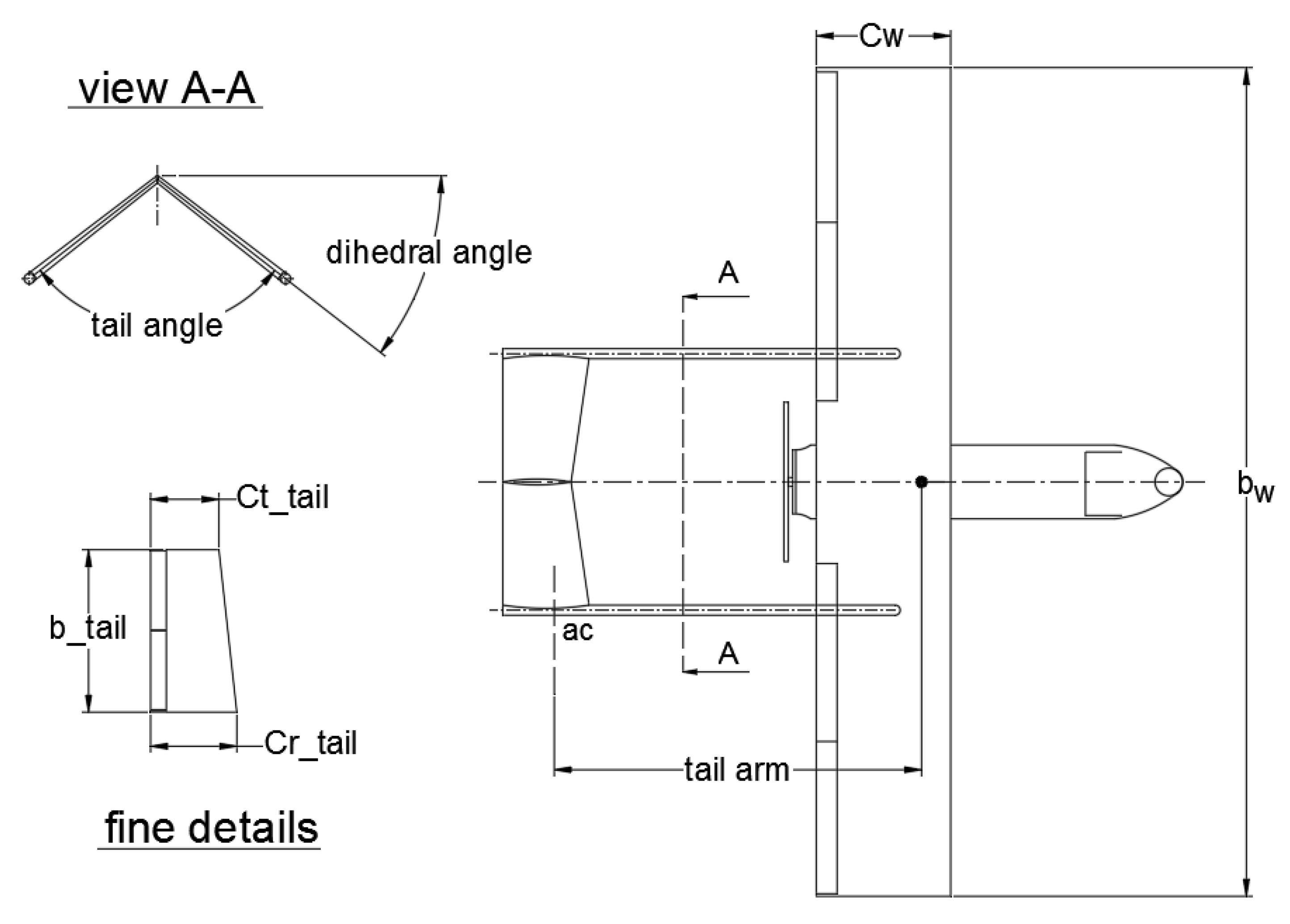
4.3. Using Wing and Tail Design Variables for Aegis UAV with Inverted V-tail Shape

We performed an optimisation in which wing-tail design variables were used simultaneously to optimise the Aegis UAV with the inverted V-tail shape. Eight design variables are used to optimise the Aegis UAV: wing span ( b w ), wing root chord ( C r _ w ), wing taper ratio ( λ w ), tail volume ( F TV ), tail arm ( L t ), inverted tail aspect ratio ( AR f ), inverted tail taper ratio ( λ f ), and inverted V-tail angle ( ϕ t ) (see Figure 8).
The problem was formulated as:
min .   f ( x ) =   min { C L 1.5 C D UAV   mass } ,
subject   to :   C L = C L
Cm ( x ) Cm
  V st ( x )     V st   0
V max ( x ) +   V max   0
  b _ hp 0.5   ( geometric   constraint )
b _ vp 0.257   ( geometric   constraint )
  b _ vp 0.445   ( geometric   constraint )
Cm α 0 ,   Cn b 0 ,   Cl b 0 ,   Cm q 0 ,   Cn r 0
x l   x   x u
x = [ b w   C r _ w   λ w   F TV   L t   AR f   λ f ϕ t ] T
where b _ hp and b _ vp are the span for the horizontal and vertical projection area for the inverted V-tail, respectively.

5. Non-Interactive and Interactive Optimisation Process

This section presents the procedure used to demonstrate the superiority of using interactive optimisation. The work started by performing a range of design scenario optimisations using the non-interactive algorithm, MOTS. The aim is to better understand the design space and provide an optimum design case for the interactive scenario (see Figure 4).

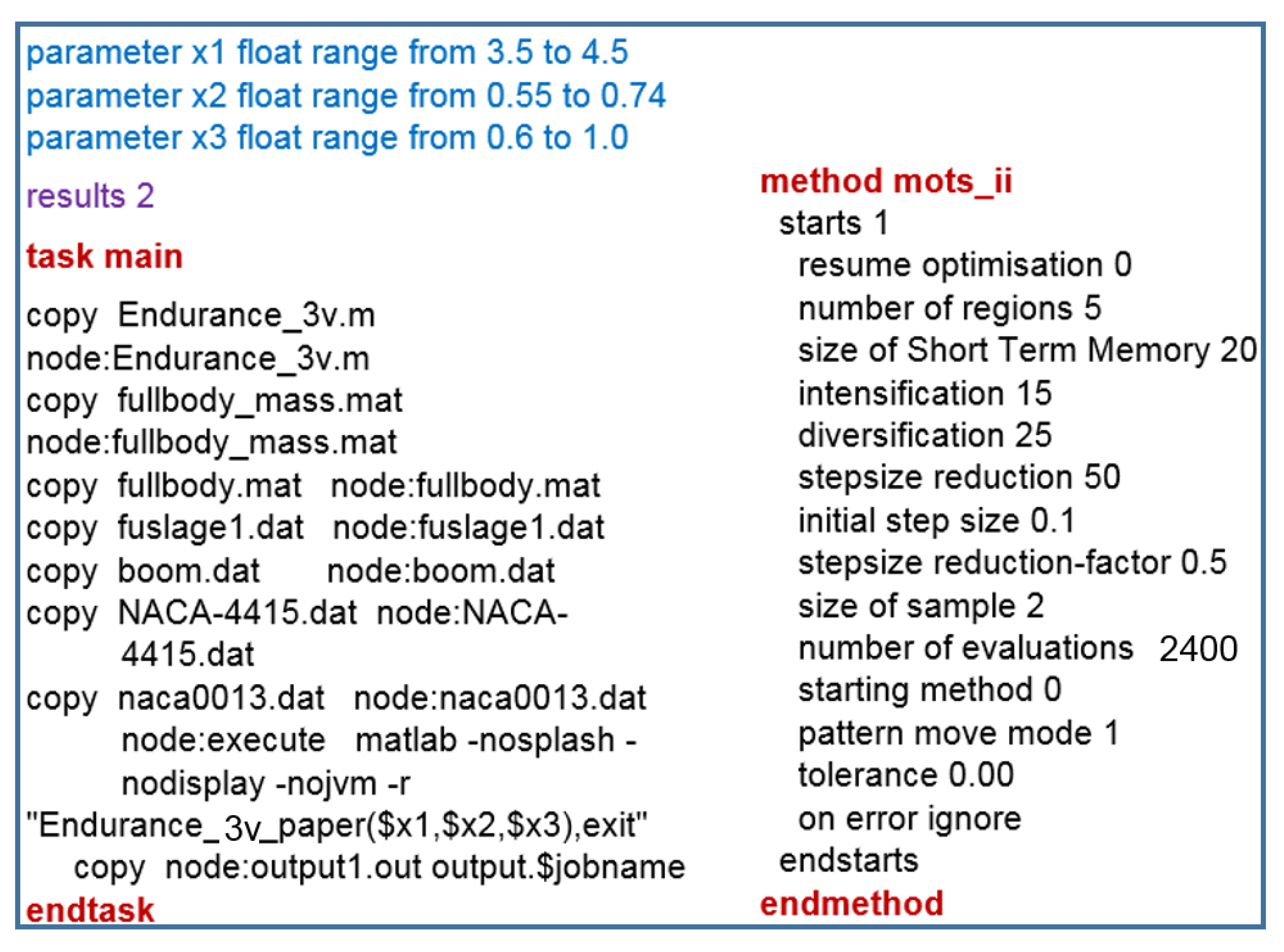
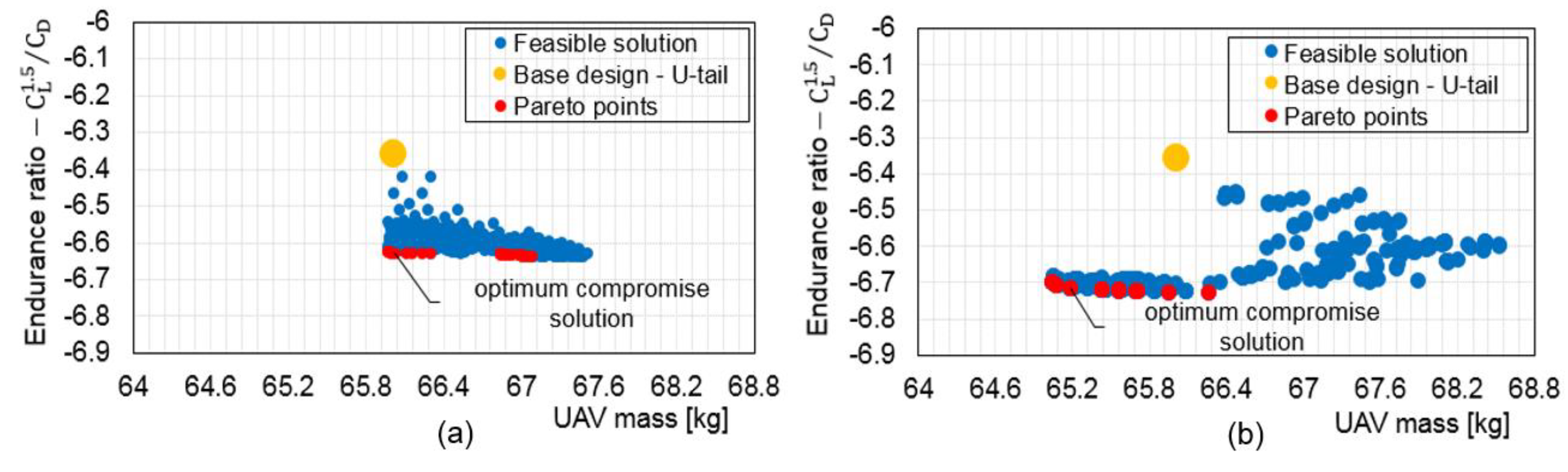
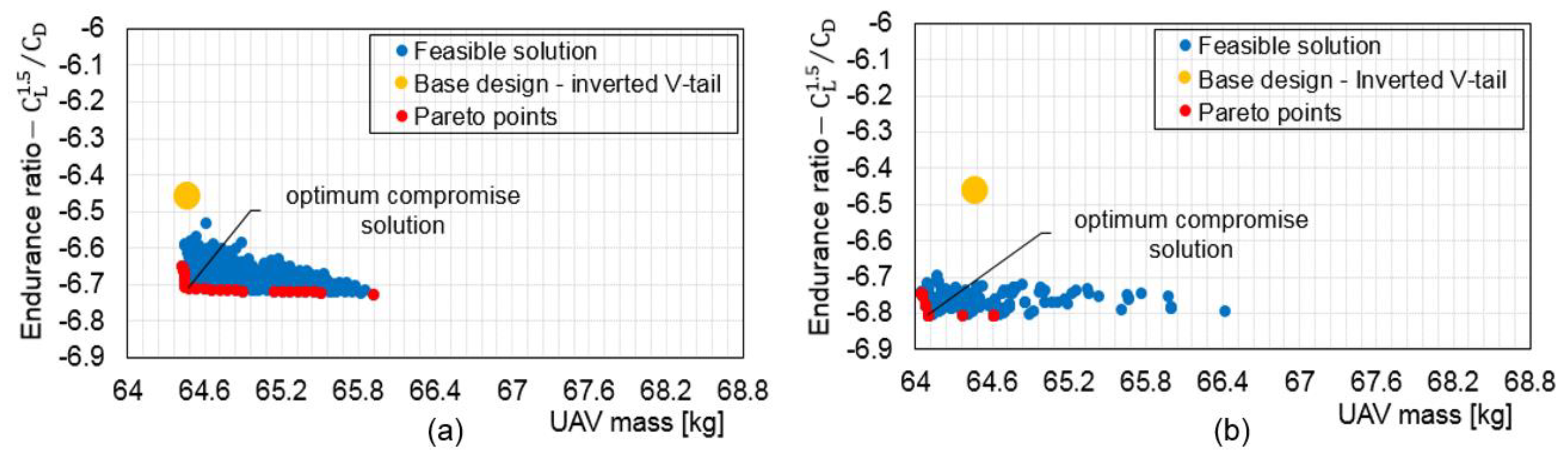
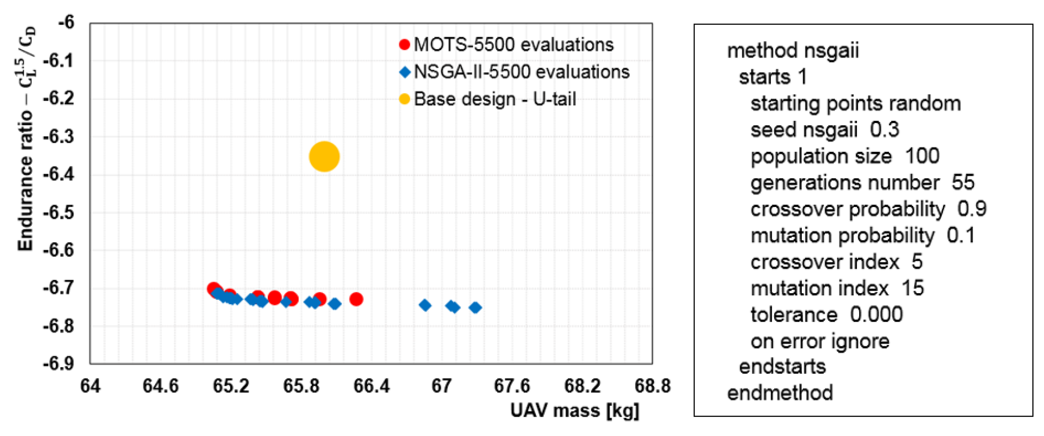
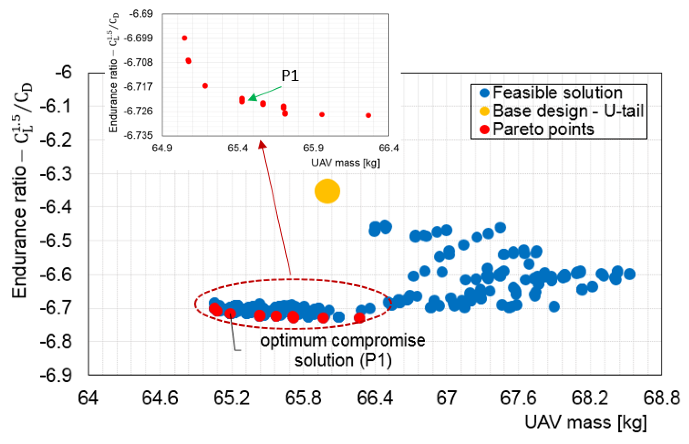
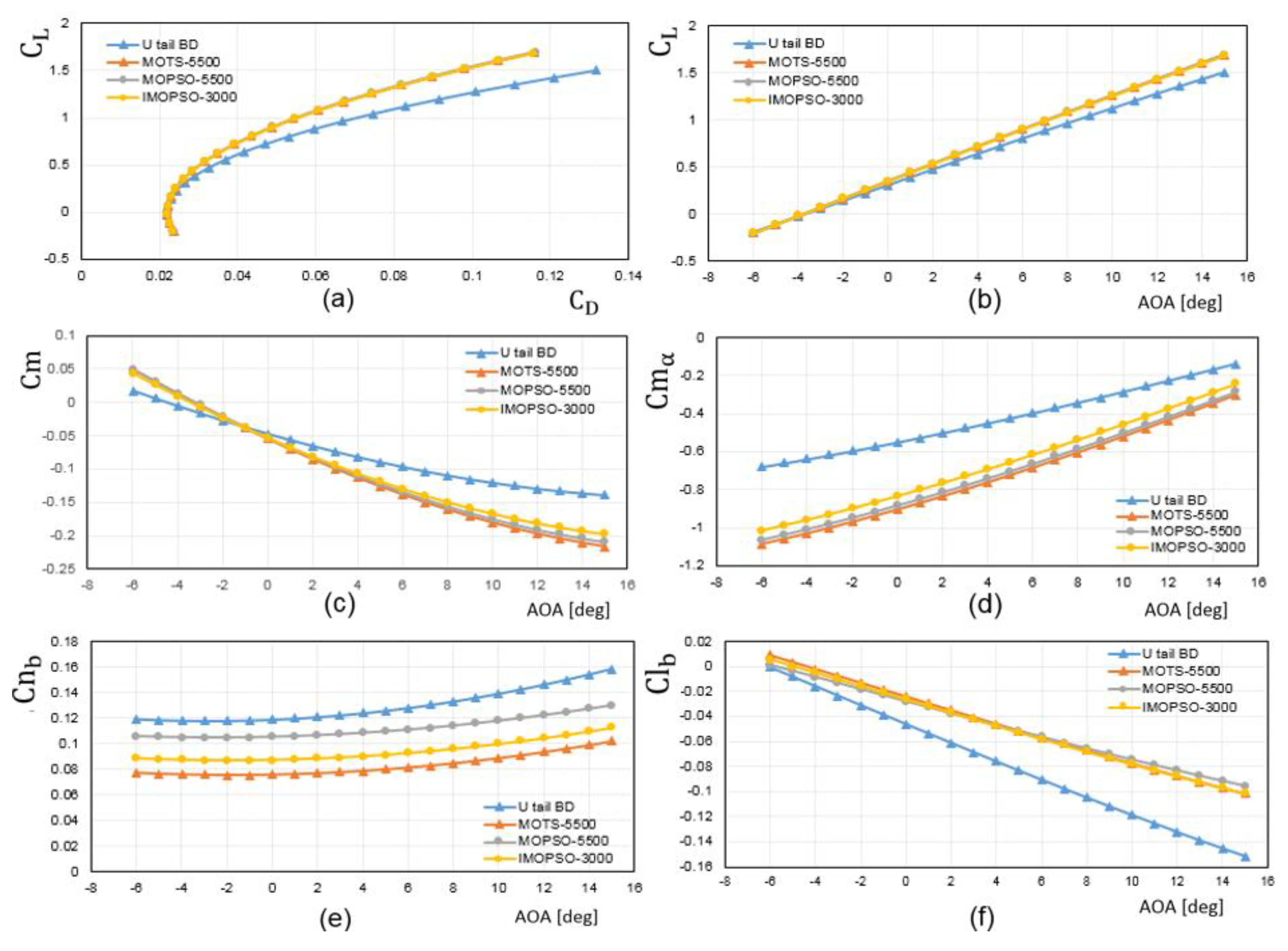
5.1. Non Interactive Optimisation (MOTS) Results and Discussion

In this section, the strategy that employs the Nimrod/O tool, as discussed in Section 2.2 and formulated in Section 4, was used to accelerate the optimisation process while exploring ranges of efficient scenarios that could be used in the aerodynamic shape design problem. This work used Nimrod/O, a tool that has previously and successfully been tested using the High-Performance Computer (HPC) at Cranfield University [38,39].
Through the non-interactive optimisation process, multiple runs were performed for each design case and the results were mostly similar, which is considered to be supporting evidence for the robustness and the suitability of using MOTS for aerodynamic shape design optimisation of aircraft in general. The MOTS algorithm setting was investigated by performing several runs with different sets of regions and evaluations [71,72]. A compromise between number of evaluations and number of regions was made. Five regions and evaluations were selected, ranging from 2400 to 5500. The compromise depended on the number of design variables.
Figure 9 and Figure 10 show the aerodynamic shape design optimisation results of the Aegis UAV with U and inverted V-tail configurations, where wing and wing-tail design variables were varied simultaneously to obtain the optimum Pareto set. The optimisation results for selected compromise solutions show that the optimised UAV with inverted V-tail shapes has a higher endurance ratio and lower mass than the optimised UAV with the U-tail shape. However, the improvements in endurance ratio and mass with respect to the base design are better in the case of the UAV with the U-tail shape. For example, the endurance ratio of the optimum compromise solutions for UAV with U-tail is improved by 4.41% and 5.83%, whereas for UAV with inverted V-tail improved by 3.89% and 5.43%, respectively, when using wing and wing-tail design variables. It is evident that combining wing and tail in the optimisation process provides better performance in both endurance ratio and UAV mass.
The improvement in the endurance ratio for the compromise solutions for both configurations of the Aegis UAV was achieved with zero reduction in the mass when the wing design variables are used. On the other side, decreases in mass of 0.91% and 0.56% were obtained with the compromise solutions for the UAV with U-tail and inverted V-tail, respectively, when the wing-tail design variables were used.
Detailed study of the obtained solutions showed that the aerodynamic design optimisation problem is highly constrained, since the number of infeasible solutions is much more than the number of feasible solutions. For example, the optimiser applied around 4903 and 4990 penalty functions on solutions that did not satisfy the constraints when the wing and tail design variables were used simultaneously to optimise Aegis UAV with U and inverted V-tail arrangements, respectively.
From the results presented in this section, we conclude that the Aegis UAV achieves the highest improvement in endurance ratio and mass with U-tail shape by optimisation of wing-tail design variables simultaneously. Thus, this case is chosen as an optimum design case to be investigated using interactive optimisation, with the aim being to reduce the computational time while retaining the high optimum solutions. However, for confirmation, the authors compared optimisation results for this design case with those obtained using the leading multi-objective Genetic Algorithmic (GA), (Non-dominated Sorting Genetic Algorithm-II (NSGA-II). Comparison supports the effectiveness of using the MOTS algorithm in such a design problem (see Figure 11).
It is obvious that both algorithms achieved almost the same quality solutions, but the non-dominated solutions obtained by NSGA-II have greater variance. On the other hand, regardless of the optimisation and search techniques used by each algorithm, the run-times for MOTS and NSGA were 135 and 142 min, respectively. This indicates that the MOTS algorithm is slightly more efficient than NSGA-II for such design problems. Overall, the MOTS algorithm exhibited better performance when compared to the leading multi-objective GA, NSGA-II.

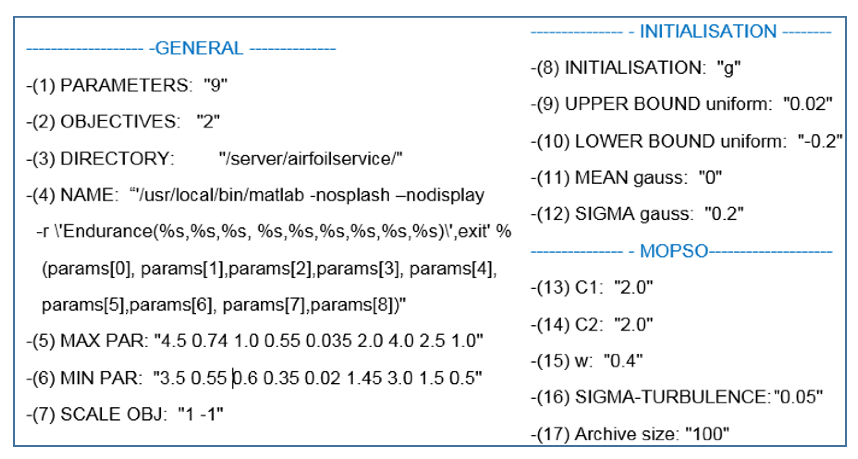
5.2. Problem Configuration of the Interactive Process

By using interactive optimisation, adding the human element to the decision-making, we aim to shorten the path for finding the optimal solution for the chosen design case. Here, we were investigating the Aegis UAV configuration with a U-tail shape by varying wing and tail design variables simultaneously (see Figure 7). This case was selected as it had the best improvement (see the right panel of Figure 9) and the highest number of design variables.
The work starts by integrating the Interface-AVL with the interactive framework, as shown in Figure 2. Two files were amended: input text file and runner.py script file. The input file is used to define the design space parameters and the algorithm characteristics, whereas the runner.py script is used to call the Interface-AVL. Figure 12 shows the input file with data used when performing the experiment interactively. To ensure a fair comparison, the experiments had the same previously used object function, design variables, upper and lower bounds, and constraints (similar to the non-interactive optimum case). For the MOPSO setting, an inertia weight of w = 0.4 and constant weightings of c 1 = c 2 = 2 were used. A Gaussian   distribution was selected to generate the initial population around the base geometry, with a mean of μ = 0.0 and a standard deviation of σ = 0.2 [6,52].
Once the I-MOPSO is executed, the code will gather the data from the input file into the various script files within the I-MOPSO framework. Next, the runner.py script will call the Interface-AVL to give the design variables after scaling and translation, and receive the values of the objective functions. The code, by default, is expected to read a list of the objectives as below.
F i n a l R e s u l t s :   [ flag   obj 1 ,   obj 2 ]
where flag can have a value of either 0 or 1, and obj1 and obj2 are the values of the objective function. The flag will be equal to 1 when the results are valid and equal to 0 when the results are invalid. An outcome is considered invalid when it does not satisfy any of the constraints. To place the invalid results far away from the valid results of the objective functions, a value of 1000 was assigned for both of the objectives when the flag was equal to zero.

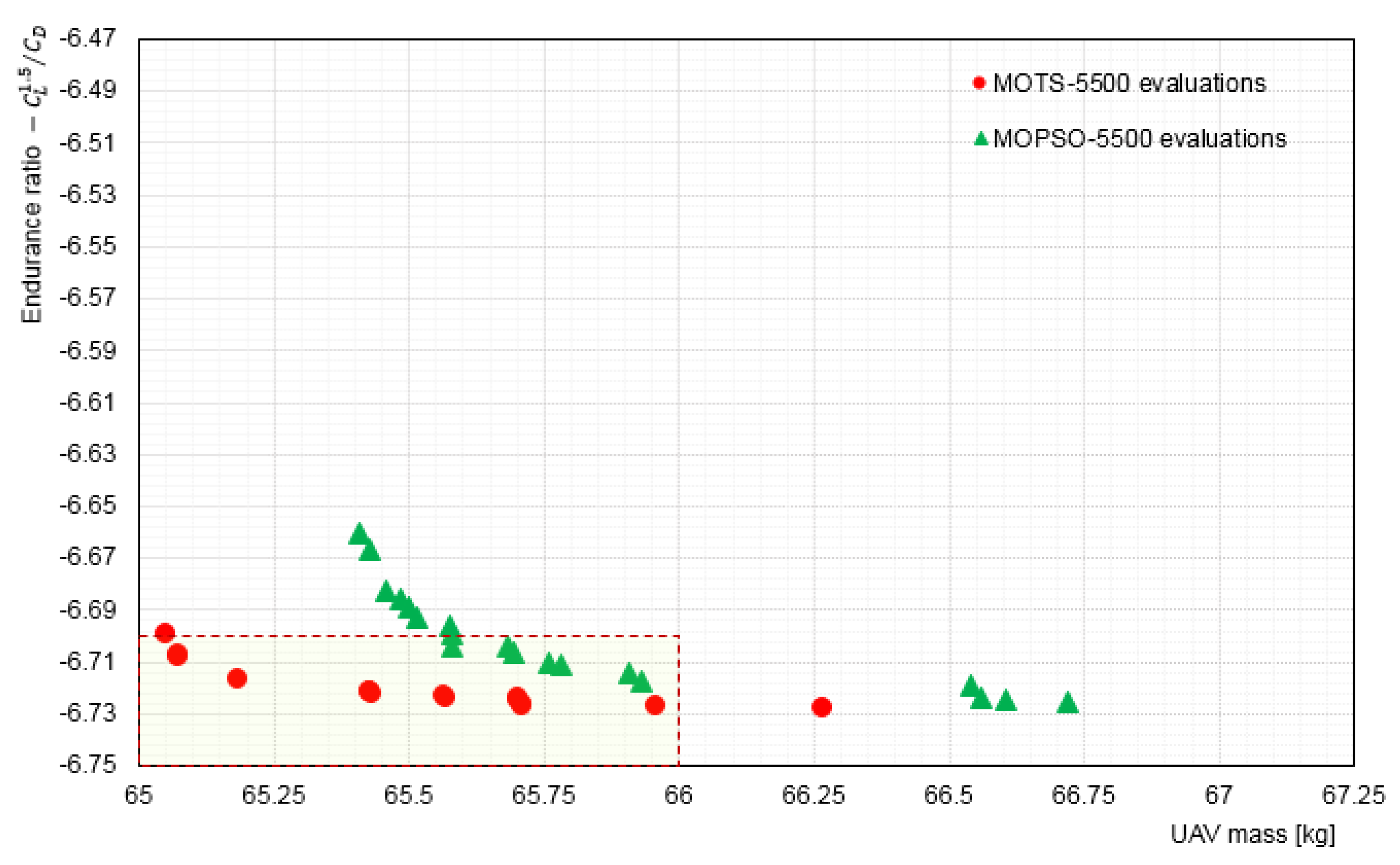
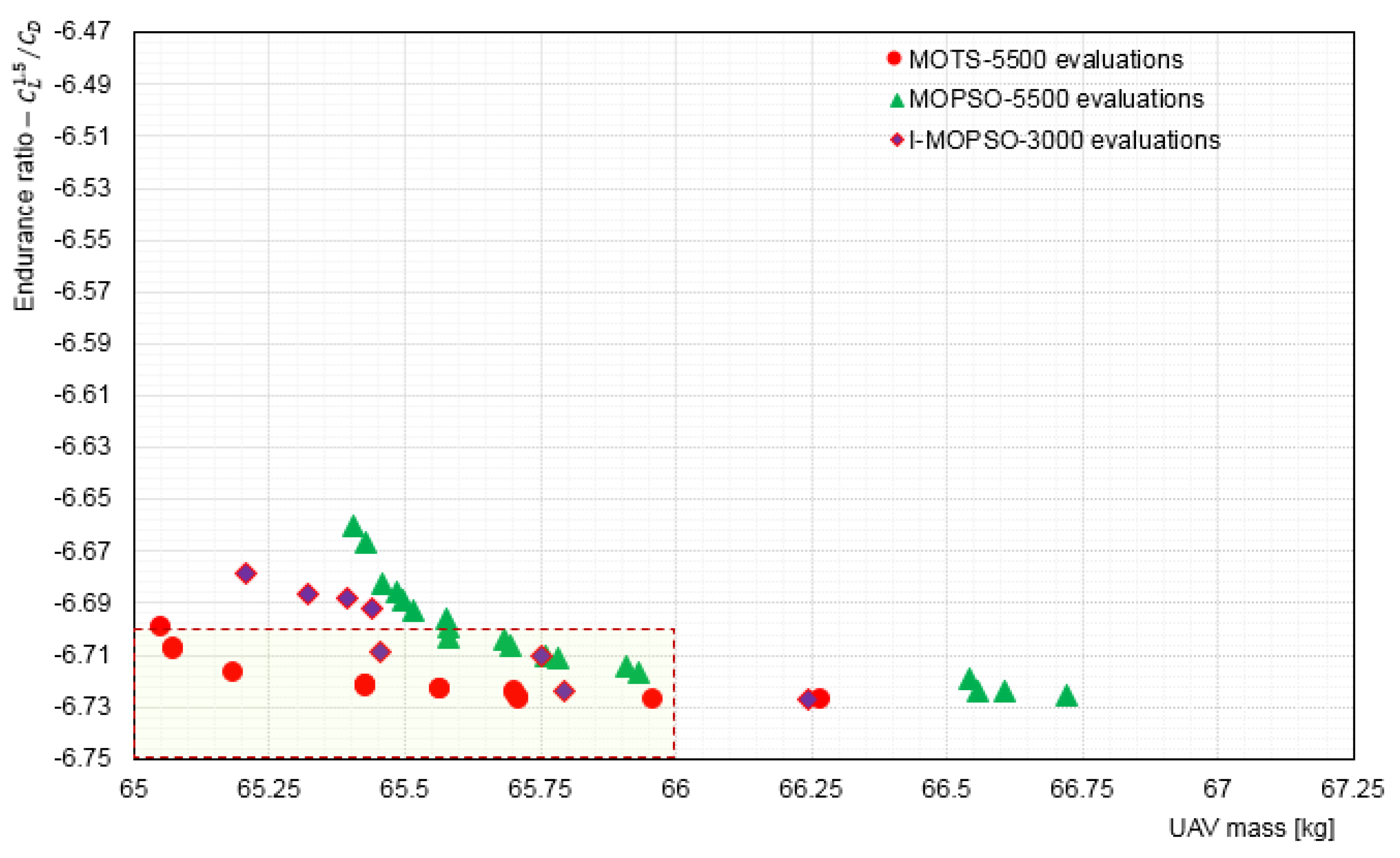
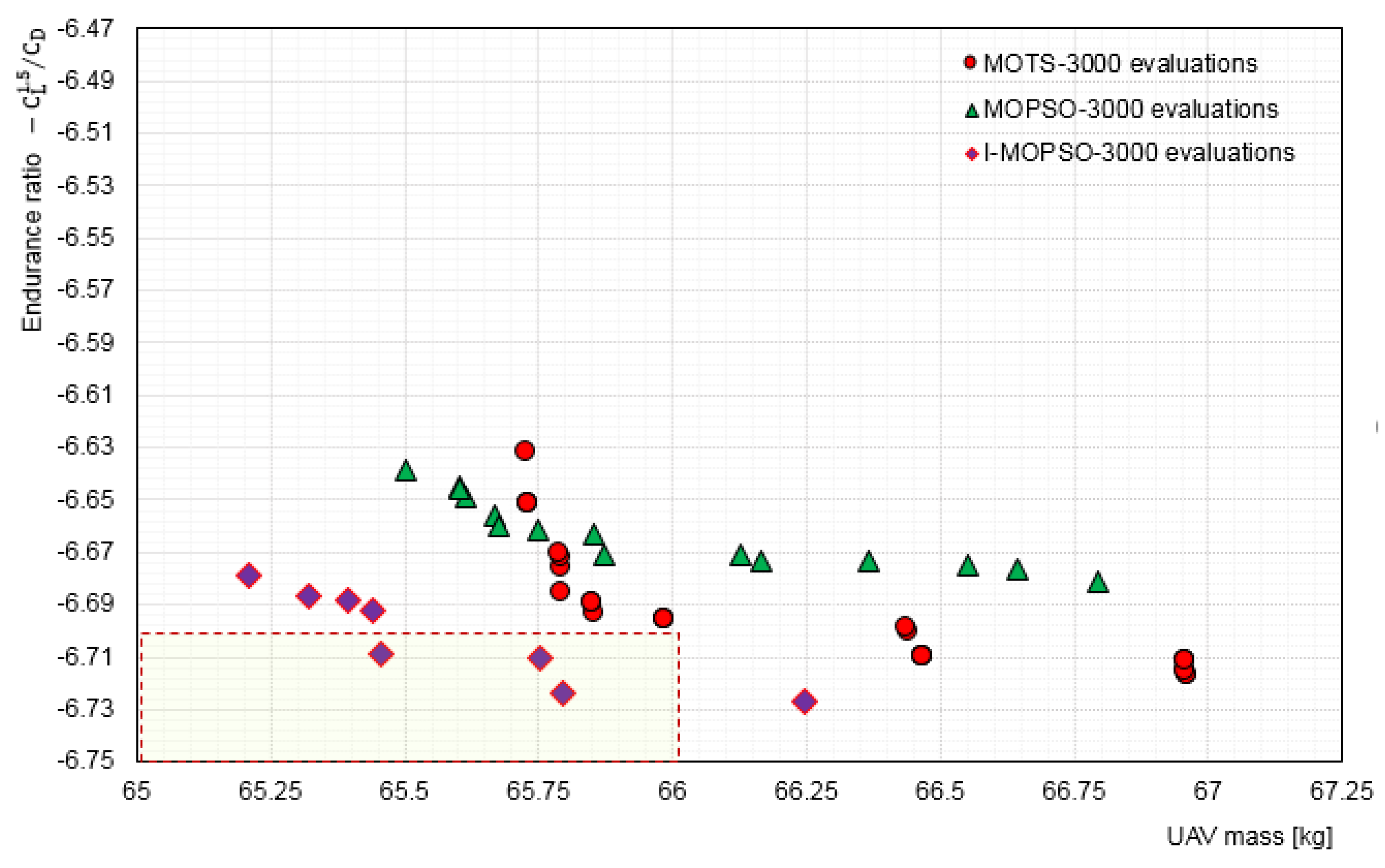
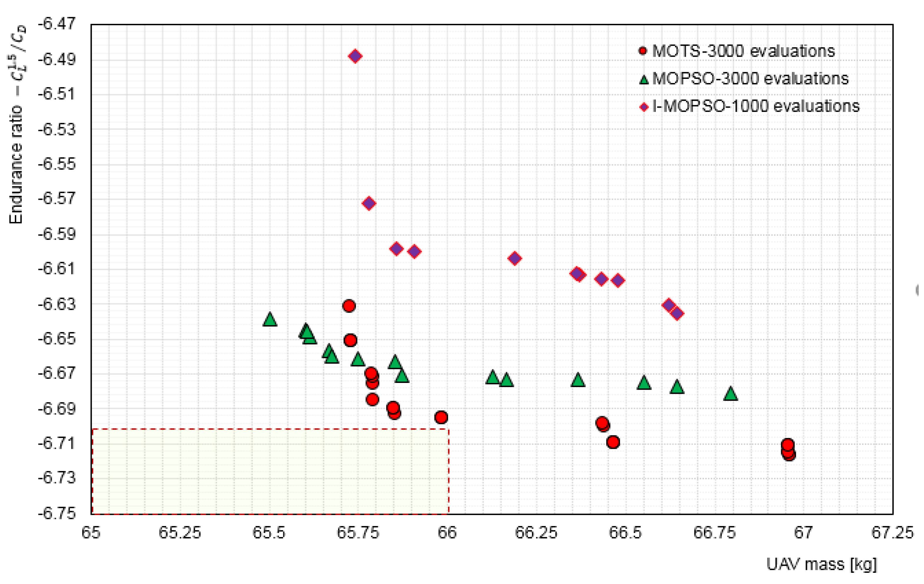
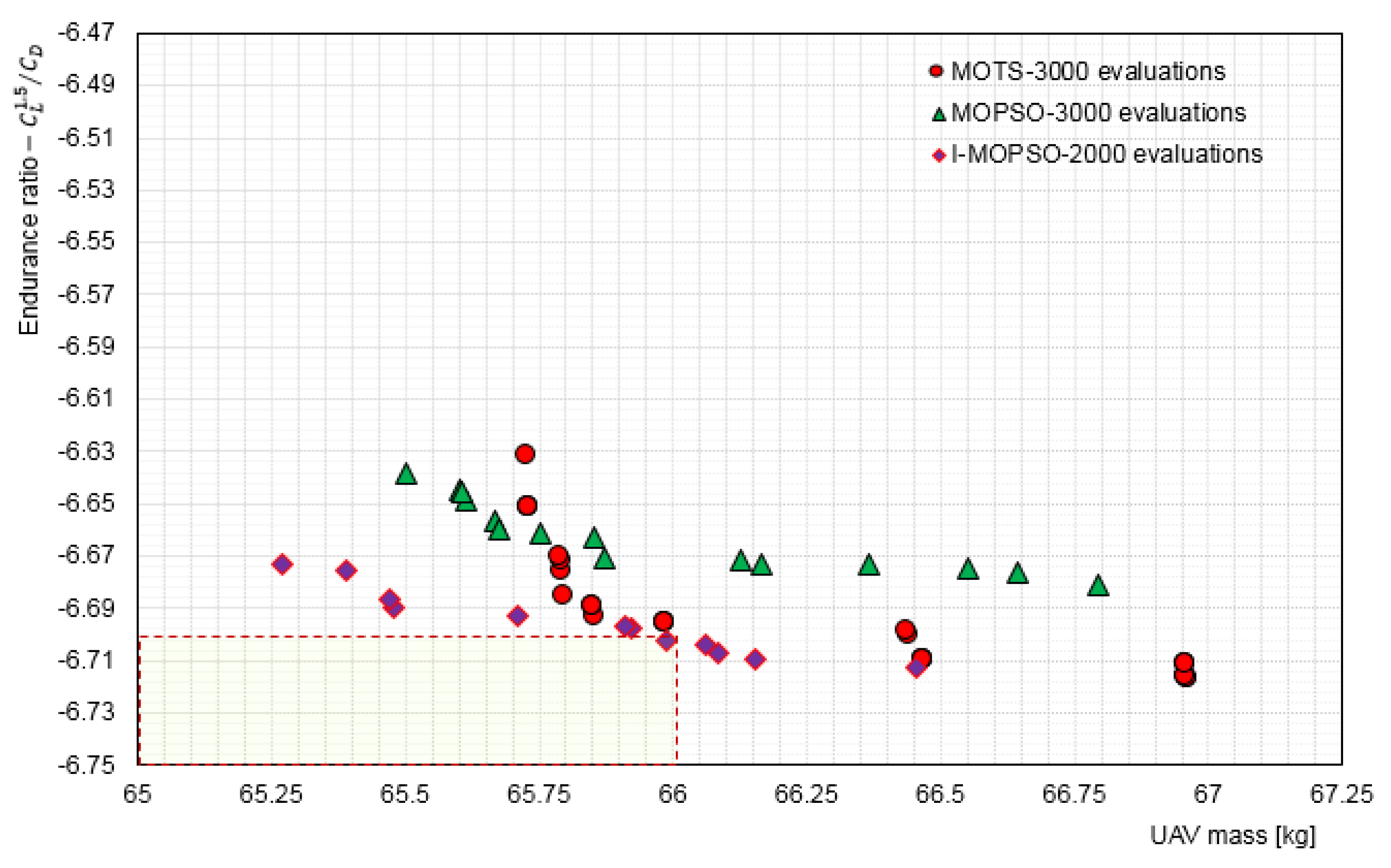
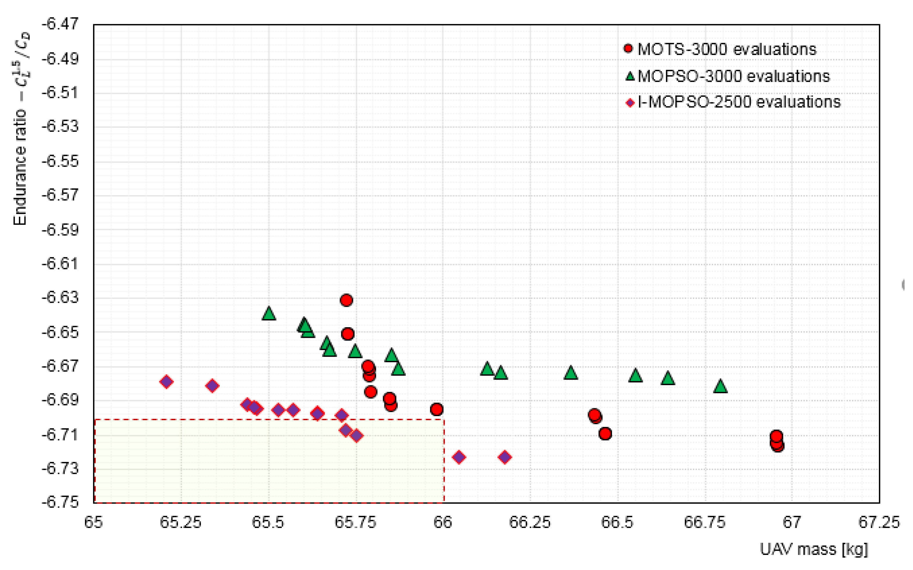
5.3. Interactive Optimisation (I-MOPSO) Results and Discussion

To demonstrate the benefit and superiority of the interactive approach (I-MOPSO), it was compared to a non-interactive approach (MOTS and MOPSO). Figure 13 shows the optimisation results obtained using the non-interactive algorithm MOTS with 5500 evaluations (see Section 5.1). From our previous results, we know that the problem is highly constrained and the number of infeasible solutions is much more than feasible solutions.
Because our algorithm, MOTS, is stochastic, we performed five runs to evaluate the optimisation performance, as shown in Figure 13. Of these five runs, on average, only 597 trial solutions were valid, and 4903 were invalid.
For the interactive runs, the DM is interested in steering the solutions to the defined ROI with a much smaller number of evaluations than used in the posterior approach (MOTS) (see Figure 13). Using fewer evaluations to find the Pareto front is very important because often each evaluation can require a significant amount of CPU time. Consequently, reducing the total number of evaluations needed has a significant impact on the time required to find an optimised design or Pareto front [71]. In this experiment, it is not suitable to compare the efficiency of the non-interactive and interactive solutions obtained using MOTS and I-MOPSO, respectively, in terms of the CPU time, since the non-interactive solutions were obtained by an algorithm running on the HPC, whereas the interactive solutions were obtained by an algorithm running on a personal computer.
The ROI was established based on our experience of optimising the Aegis UAV for different cases using the MOTS algorithm. However, obtaining similar results to Figure 13 with around half of the evaluations will be a significant result in our case. The limitations for the ROI were defined as:
f 1 = C L 1.5 C D 6.7 ( Endurance   ratio   objective )
f 2 = UAV   mass 66.0   kg   ( UAV   mass   objective )
To discover and examine the visualisation tools implemented in the obtained framework shown in Figure 2, several runs were executed, both interactive and non-interactive, using various combinations of iterations and particles. The aim is to understand all the features and controls that appear on the interactive screen, to obtain an idea of an adequate number of particles and iterations, and whether it is better to increase the number of particles or iterations during an evaluation. Even though this comparison is not the goal in this work, it was necessary to obtain an assessment of an efficient number of particles and iterations in each run for optimisation, whether interactive or non-interactive, using the MOPSO.
Once the preliminary study concerning I-MOPSO-AVL performance was completed, interactive and non-interactive optimisation results were compared in order to highlight the reduction of computational time while achieving similar or even better results. As discussed above, the DM, by interactive optimisation, attempted to deliver solutions identical to the one obtained using MOTS for 5500 evaluations with fewer evaluations. Firstly, a comparison of non-interactive MOPSO and MOTS for 5500 evaluations was performed. Considering the stochastic characteristics of the MOPSO algorithm, ten independent runs using the same algorithm setting were carried out. The non-interactive MOPSO evaluations (5500) were divided into 110 iterations with a swarm population of 50 (particles). The average run time was 195 min. Next, the best case was compared with the previous results from MOTS (see Figure 14). To some extent, the MOTS algorithm showed better performance than the non-interactive MOPSO, and it is obvious that using I-MOPSO to achieve solutions that are similar to the one obtained by MOTS with fewer evaluations will be a challenging task for the DM. In Figure 14, the red dashed box represents the ROI when performing the optimisation interactively.
The next step was to begin interactive optimisation to obtain solutions within the ROI. The interaction with the optimiser began after 15 iterations, since the non-interactive results show that only a few particles were able to satisfy the applied constraints within the first 10 iterations. By adding the human element to the interaction, we aim to shorten the path for finding the optimal solution, i.e., less time-consumed and a significant reduction in project costs. The obtained results show that when the number of evaluations reached 2000, the DM began to produce results inside the ROI. To obtain more solutions within the ROI, the number of evaluations was increased to 3000. Figure 15 compares the optimisation results using MOTS and MOPSO for 5500 evaluations, and with I-MOPSO for 3000 evaluations. With the latter, the DM, using only 3000 evaluations, was able to guide the optimisation process to within the ROI. Steering the optimisation process to the ROI prevents the algorithm wasting time exploring the whole design space. This approach consumes less time, while providing a more flexible approach for any design problem. The DM spent around 130 min to satisfy the constraints and steer the search to the ROI (33.4% reduction in the computational time compared to non-interactive MOPSO using 5500 evaluations).
An additional demonstration of the superiority of undertaking optimisation interactively is presented in Figure 16, which shows a comparison of interactive and non-interactive results for MOTS and MOPSO with I-MOPSO, all for 3000 evaluations. The superiority of interactive optimisation is evident. The non-interactive results from MOTS and MOPSO were not able to generate solutions inside the ROI, whereas including the DM in the optimisation process allows the search to focus on the area of the Pareto front that is of interest.
In fact, with interactive optimisation, the DM does not need to continue the optimisation process to the end, since it is able to stop the simulation at any iteration that gives a solution that satisfies the design requirements. Figure 17, Figure 18 and Figure 19 demonstrate the dynamic behaviour of the Pareto front at 1000, 2000, and 2500 evaluations.
It was evident that at 1000 evaluations the Pareto solutions cover a vast design space, then as the iterations increased, the solutions accelerated quickly to cover less design space. This is because the DM pushed the optimiser to focus on the solutions that appear within the correlation, and ignore other points that are not of interest. Of course, the DM benefitted from both visualisation tools available on the interface screen and Parallel and Scatter Cartesian coordinates to guide the simulation to the desired region for the interactive solutions. Furthermore, Figure 19 shows clearly that the simulation can benefit from interactive optimisation, since the solutions are within the ROI with only 2500 evaluations (simulation time was around 100 min). It is evident that interactive optimisation accelerated the optimisation process and achieved optimal results. Thus, integrating the DM with the optimisation search enabled faster convergence to the optimal solution.

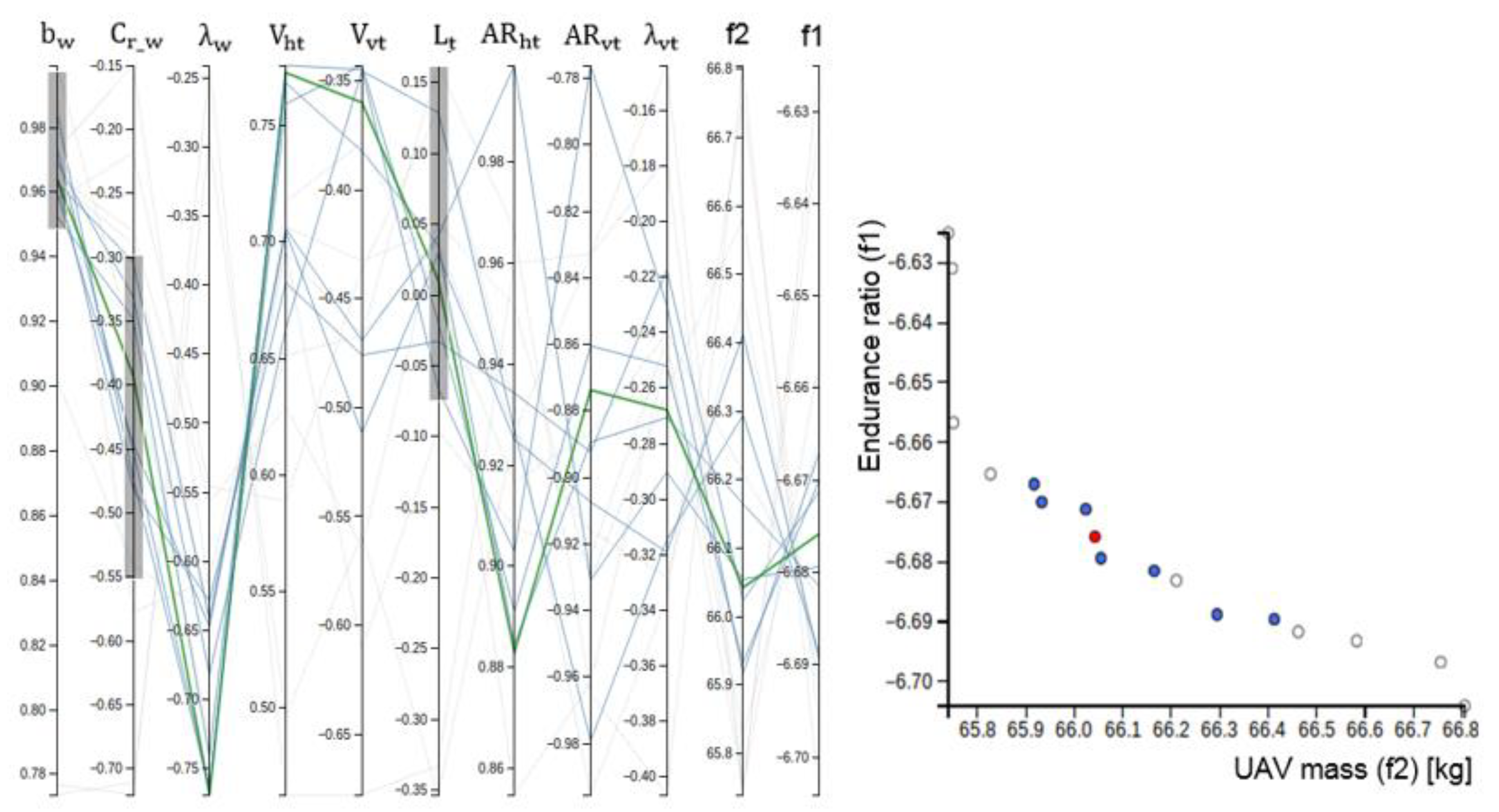
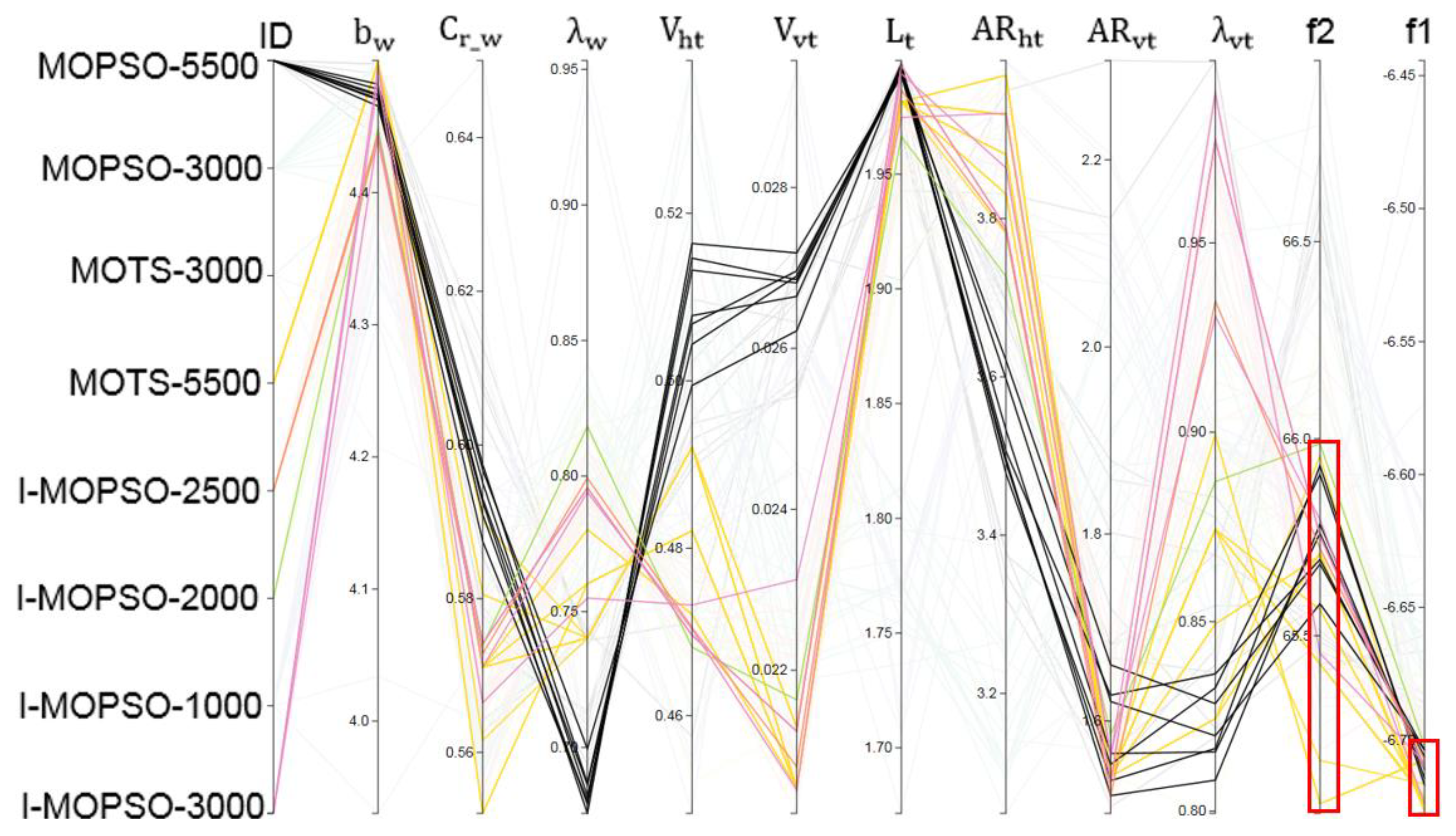
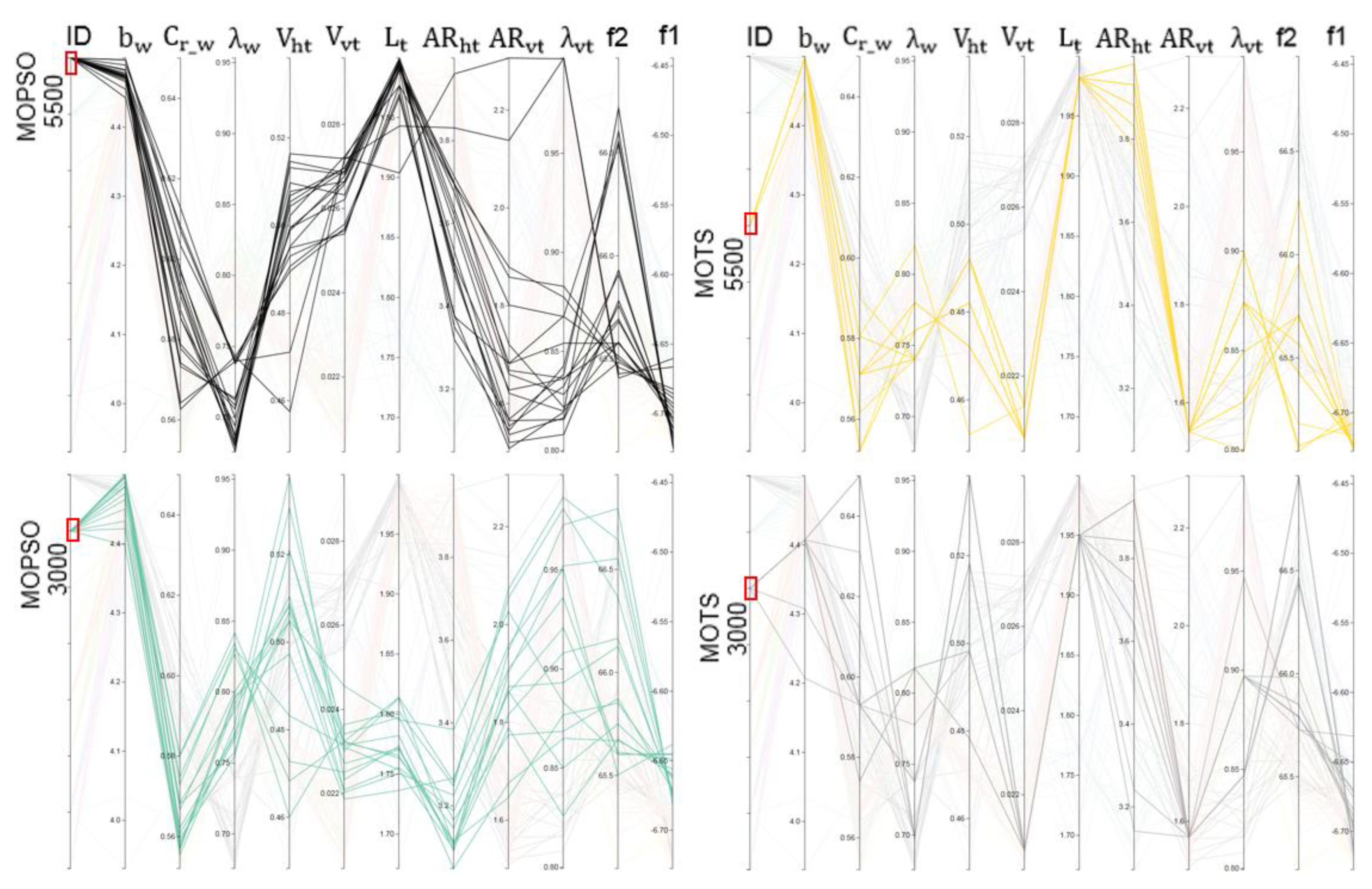
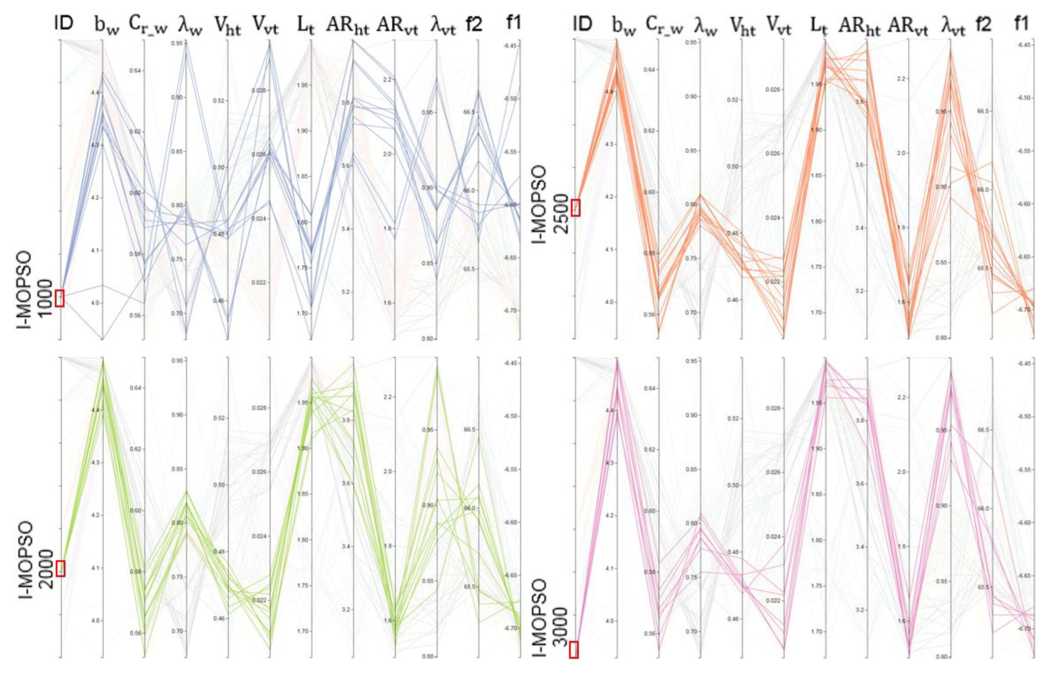
5.3.1. Visualisation of Results Using Parallel Coordinates

Parallel Coordinates has been shown to be a good technique for visualisation, analysis, and the study of large amounts of data [42]. This approach allows observation of the relations between design variables, trade-offs between objective functions, and can monitor the evaluation process [49,73,74]. Furthermore, such a visualisation tool can be used to display the characteristics of a trend, and correlations that exist among and between the design space parameters [75]. Figure 20 shows a comparison of the results for various optimisation scenarios used in this work—MOTS for 5500 and 3000 evaluations, non-interactive MOPSO also for 5500 and 3000 evaluation, and I-MOPSO for 1000, 2000, 2500, and 3000 evaluations. It is obvious that by using the Parallel Coordinates techniques, the DM can highlight the number of runs that satisfies the constraints (ROI), which are highlighted when the ROI is selected (see the two red rectangular boxes in Figure 20 that represent the objective functions).
Generally, the achieved trends display the correlation that exists between the design variables and the objectives. Besides, such an approach helps the understanding of the influence of the design variables in combination on the solutions within the ROI. Thus, the DM can now relatively easily identify the effective range for each design variable. Also, it becomes clearer which are the design variables with limited range or a range wide enough to satisfy the design requirements. In fact, it is a responsibility of the DM to select which solutions best fit the requirements for the next stage of the design.
For example, visualisation and analysis of the results displayed using Parallel Coordinates give more details about values of the design variables that participate in achieving high-performance solutions. It was clear that the maximum values of span ( b w ) and boom length ( L t ) always participated in provision of high performance (results within the ROI). However, there was more scope to vary the values of the design variables—vertical tail taper ratio ( λ v t ) , horizontal tail volume ( V h t ) , and vertical tail volume ( V v t ) —and still maintain high performance. In fact, this is the idea behind multi-objective optimisation—several conflicting objectives are optimised simultaneously as a function of various design variables and constraints to identify non-dominated solutions (since there is no single optimal solution). It is a DM’s job to analyse the non-dominated solutions to select the most appropriate solution satisfying its requirements.
To obtain optimal geometry for the UAV with respect to wing and tail design variables simultaneously, the optimiser had to find compromise solutions that included both wing surface area and tail volume [15,54]. Wing sizing is related to tail sizing, which has as its primary function the simultaneously countering of the moments that will be produced by the wing, and also satisfying stability requirements.
Visualisation of the results shows the difference in the ability of the optimisation algorithms to meet these requirements. For example, when the MOPSO for 5500 evaluations selected higher values of vertical and horizontal tail volumes (higher tail volume, i.e., surface tail area multiplied by arm length), the obtained total mass ( f 2 ) was higher than that obtained by MOTS for 5500 and I-MOPSO for 3000 evaluations. However, the optimiser in this case (MOPSO-5500) was trying to reduce the weight and improve the endurance ratio because low values for wing taper ratio ( λ w ) and vertical tail taper ratio ( λ vt ) had been selected. On the other hand, MOTS for 5500 and I-MOPSO for 3000 evaluations selected almost identical values of the design variables that satisfy the requirements of optimum objective functions. Note, however, that the vertical tail taper ratio ( λ vt ) was obviously not identical for both algorithms. The lower UAV mass ( f 2 ) obtained by MOTS for 5500 evaluations is a direct confirmation of the previous results. However, it is very evident that interactive optimisation with 3000 evaluations provided very competitive results when compared to the results obtained for 5500 evaluations using either MOPSO or MOTS.
In spite of the successes obtained using interactive optimisation, we noticed that the interactive solutions (Pareto solutions) are concentrated around certain values of each design variable, whereas non-interactive solutions were more widely spread. As a result, each Pareto solution for the non-interactive process consists of diverse values for the design variables, which is preferred by the designer [9]. In addition, the non-interactive solutions were obtained by exploring a wide range of the design spaces, whereas in the interactive approach, the search is steered by the DM once the run is started, providing solutions obtained by less exploration of the design space (see Figure 21 and Figure 22). In fact, this is the major penalty for interactive optimisation; we may miss information in the design space despite the fact that we are achieving high optimality corresponding to our design requirements in much less computational time, which is the primary focus of the DM in this case.

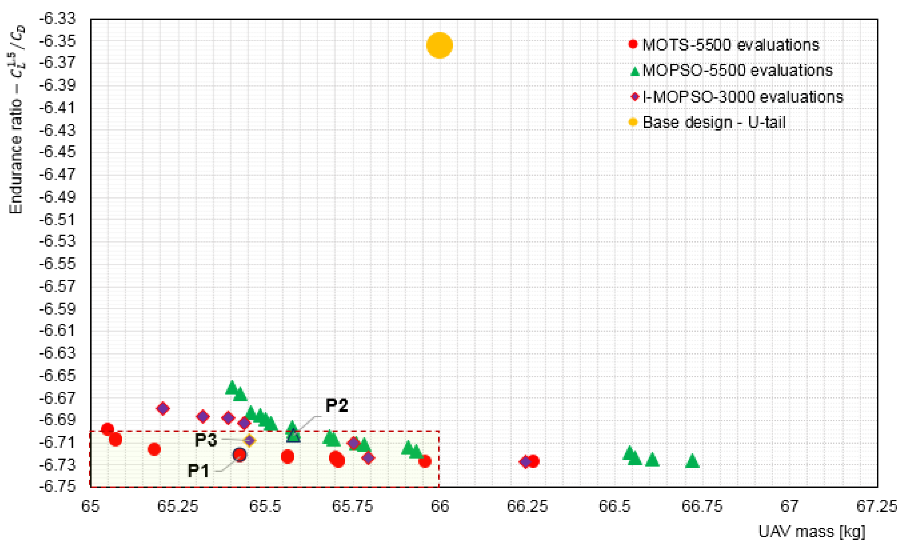
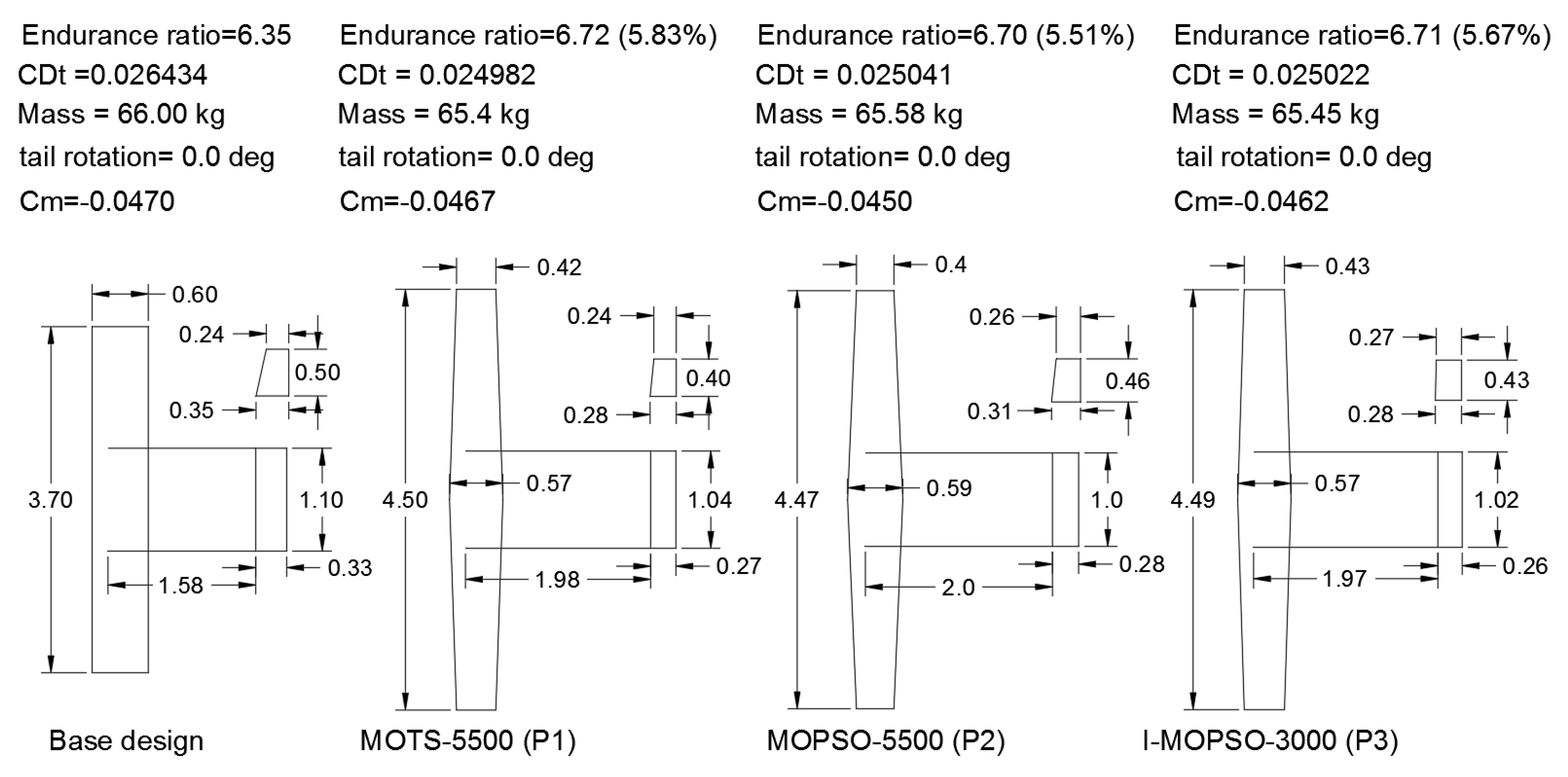
5.3.2. Investigation of Selected Configurations

Finally, selected configurations from non-dominated solutions were considered for further analysis. Figure 23 compares the full Pareto Front, obtained using MOTS and MOPSO for 5500 evaluations and I-MOPSO for 3000 evaluations. A visual inspection of the Pareto front for each run can provide useful information to DMs about the possible trade-offs between objectives. Configurations P1 (MOTS-5500), P2 (MOPSO-5500), and P3 (I-MOPSO-3000) were selected as compromise solutions, since we have the same interest in minimising both objectives. It is obvious that P3 provided better improvements than P2 in endurance ratio and UAV mass. On the other hand, P1 showed a slightly better improvement in the endurance ratio and UAV mass than P3. However, it must be kept in mind that P3 was obtained with only 3000 evaluations, compared to 5500 evaluations for P1 and P2.
Figure 24 shows the geometry of the selected compromise solutions and the performance of each one numerically. In fact, all the optimised configurations have a similar performance. The interactive compromise solution P3 has a drag 5.34% lower than that for the base design geometry, while P1 and P2, respectively, have a drag that was 5.49% and 5.27% lower than that for the base design. The drag decreased from 264.3 counts for the base design to 249.8, 250.2, and 250.4 counts, respectively, for P1, P3, and P2 at level flight. Furthermore, the optimised configurations using either I-MOPSO or MOPSO have a lower absolute value of pitching moment than the P1 configuration, and so will gain a lower increment of drag when better trimmed for level flight, which should lead to better performance.
As a further study, the aerodynamic characteristics for each of the optimised configurations and base design were simulated for different angles of attack (see Figure 25). It is obvious the configuration obtained by I-MOPSO has a high lift to drag ratio for all angles of attack, which coincides with the other optimised configurations. All configurations are stable longitudinally, laterally, and directionally. It is evident that interactive optimisation requires less computational time and does not degrade the aerodynamic performance of the optimised configurations. Appendix A provides the reader with details about the panels and planes for one configuration, as structured within the AVL setup file.

6. Conclusions

This work has investigated the efficiency and effectiveness of interactive optimisation in the design of the aerodynamic shape of the Aegis UAV with U-tail. The proposed framework is flexible and able to obtain high optimality solutions in shorter computational times. It combines I-MOPSO with a low fidelity flow solver, AVL. We compared the interactive results for I-MOPSO with non-interactive results for MOPSO and MOTS algorithms for the whole UAV with U-tail. The obtained results using interactive optimisation show the ability of the DM to use its preferences effectively to steer the search to the ROI without degrading the aerodynamic performance of the optimised configurations. Even using only half the number of evaluations, the DM was able to obtain results similar to those obtained by a posteriori approaches. An advantage was that it was possible for the DM to stop the search at any iteration, which is not possible in a posteriori approaches even when solutions do not converge or may be infeasible.
The increase in performance is accompanied by a significant reduction in computational time. For example, comparing the interactive and non-interactive results obtained using the MOPSO algorithm shows that by almost halving the number of total evaluations, the computational time has been cut by a third (33.4%). Each 5500-evaluation run (non-interactive) required about 195 min to be completed, whereas each 3000-evaluation run (interactive) took around 130 min. The computational time used by the interactive approach includes the time required by the DM to interact with the optimisation search. The fall in computational time is, in fact, remarkable.
In spite of the successes obtained using interactive optimisation, interactive solutions were concentrated within a limited range for each design variable, whereas non-interactive optimisation solutions were widely spread. Thus, there is the possibility that interactive optimisation may miss some important information regarding the design space, despite achieving high optimality corresponding to the design requirements in substantially less computational time, which was a primary aim of the DM in this case. Future work has begun on enhancing the optimisation results, using an Artificial Neural Network performing deep space exploration to retain all the useful information of the design space in adequate computational time with high optimality.

Author Contributions

Y.A. performed all the simulations and work in this manuscript. A.S. and T.K. provided the guidance and feedback on the results presented in this paper.

Funding

This research received no external funding.

Conflicts of Interest

The authors declare no conflict of interest.

Nomenclature

AOA= Angle of attack
E= Endurance ratio
UAV= Unmanned Aerial Vehicle
UAV   mass = UAV total mass
AR f , AR ht , AR vt = Inverted V-tail, horizontal tail, and vertical tail aspect ratio
ac = Aerodynamic center
b w , C r _ w = Wing span and wing root chord
bvt , bht = Vertical and horizontal tail span
b _ tail = Inverted V-tail span
b _ hp , b _ vp = Span for the horizontal and vertical projection area for the inverted V-tail
C D , C L , Cm= Drag, lift, and pitch moment coefficient
Cht = Horizontal tail chord
Ct _ vt , Cr _ vt = Vertical tail tip and root
Ct _ tail , Cr _ tail = Inverted V-tail tip and root
Cm α = Pitching moment slope
Cl b , Cn b = Variation of rolling and yawing force coefficient with sideslip angle
Cm q = Variation of pitching moment coefficient with pitch rate
Cn r = Variation of yawing force coefficient with yaw rate
C L , Cm = Base design lift and pitching moment coefficient
F TV = Inverted V-tail volume
L t = Tail arm
n/a = Not applicable
V ht , V vt = Horizontal tail and vertical tail volume
V st , V max = Optimised UAV stall velocity and maximum velocity
V st , V max = Base design stall velocity and maximum velocity
x = Design variable
x l , x u = Lower and upper bounds of the design variables
λ w ,   λ vt ,   λ f = Wing, vertical tail, and inverted V-tail taper ratio
ϕ t = Inverted V-tail angle
Γ _ tail = Dihedral angle

Appendix A

This Appendix presents an overview of AVL input file for a selected optimised configuration.
Figure A1. An explanatory geometry input file. It is a compulsory file to perform analysis in Athena Vortex Lattice (AVL). Here, it describes the Aegis UAV configuration obtained using interactive optimisation for 3000 evaluations.
Aerospace 06 00042 g0a1

References

  1. Crombecq, K.; Laermans, E.; Dhaene, T. Efficient space-filling and non-collapsing sequential design strategies for simulation-based modeling. Eur. J. Oper. Res. 2011, 214, 683–696. [Google Scholar] [CrossRef]
  2. Goertz, S.; Ilic, C.; Jepsen, J.; Leitner, M.; Schulze, M.; Schuster, A.; Scherer, J.; Becker, R.; Zur, S.; Petsch, M. Multi-Level MDO of a Long-Range Transport Aircraft Using a Distributed Analysis Framework. In Proceedings of the 18th AIAA/ISSMO Multidisciplinary Analysis and Optimization Conference, Denver, CO, USA, 5–9 June 2017; pp. 1–24. [Google Scholar] [CrossRef]
  3. Leifsson, L.; Koziel, S.; Bekasiewicz, A. Fast low-fidelity wing aerodynamics model for surrogate-based shape optimization. Procedia Comput. Sci. 2014, 29, 811–820. [Google Scholar] [CrossRef]
  4. Jameson, A. Re-Engineering the Design Process through Computation. J. Aircr. 1999, 36, 36–50. [Google Scholar] [CrossRef]
  5. Rao, R.; Rai, D.; Balic, J. A multi-objective algorithm for optimization of modern machining processes. Eng. Appl. Artif. Intell. 2017, 61, 103–125. [Google Scholar] [CrossRef]
  6. Hettenhausen, J.; Lewis, A.; Randall, M.; Kipouros, T. Interactive Multi-Objective Particle Swarm Optimisation using Decision Space Interaction. In Proceedings of the IEEE Congress on Evolutionary Computation, Cancun, Mexico, 20–23 June 2013. [Google Scholar]
  7. Branke, J.; Greco, S.; Słowiński, R.; Zielniewicz, P. Interactive evolutionary multiobjective optimization driven by robust ordinal regression. Bull. Pol. Acad. Sci. Tech. Sci. 2010, 58, 347–358. [Google Scholar] [CrossRef]
  8. Deb, K.; Sinha, A.; Korhonen, P.J.; Wallenius, J. An interactive evolutionary multiobjective optimization method based on progressively approximated value functions. IEEE Trans. Evol. Comput. 2010, 14, 723–739. [Google Scholar] [CrossRef]
  9. Nebro, A.J.; Ruiz, A.B.; Barba-González, C.; García-Nieto, J.M.; Luque, M.; Aldana-Montes, J.F. InDM2: Interactive Dynamic Multi-Objective Decision Making using evolutionary algorithms. Swarm Evol. Comput. 2018, 40, 184–195. [Google Scholar] [CrossRef]
  10. Özmen, M.; Karakaya, G.; Köksalan, M. Interactive evolutionary approaches to multiobjective feature selection. Int. Trans. Oper. Res. 2018, 25, 1027–1052. [Google Scholar] [CrossRef]
  11. Fleming, P.J.; Purshouse, R.C. Many-objective optimization: An engineering design perspective. In International conference on evolutionary multi-criterion optimization; Springer: Berlin/Heidelberg, Germany, 2005; pp. 14–32. [Google Scholar]
  12. Li, K.; Chen, R.; Savic, D.; Yao, X. Interactive Decomposition Multi-Objective Optimization via Progressively Learned Value Functions. Neural Evol. Comput. 2018, arXiv:1801.00609. [Google Scholar]
  13. Hettenhausen, J.; Lewis, A.; Mostaghim, S. Interactive multi-objective particle swarm optimization with heatmap-visualization-based user interface. Eng. Optim. 2010, 42, 119–139. [Google Scholar] [CrossRef]
  14. Ninian, D.; Dakka, S. Design, Development and Testing of Shape Shifting Wing Model. Aerospace 2017, 4, 52. [Google Scholar] [CrossRef]
  15. Lyu, Z.; Kenway, G.K.W.; Martins, J.R.R.A. Aerodynamic Shape Optimization Investigations of the Common Research Model Wing Benchmark. AIAA J. 2015, 53, 968–985. [Google Scholar] [CrossRef]
  16. Leifsson, L.; Koziel, S. Simulation-Driven Aerodynamic Design Using Variable-Fidelity Models; World Scientific: London, UK, 2015. [Google Scholar]
  17. Quagliarella, D.; Della Cioppa, A. Della Genetic algorithms applied to the aerodynamic design of transonic airfoils. J. Aircr. 1995, 32, 889–891. [Google Scholar] [CrossRef]
  18. Lyu, Z.; Martins, J.R.R.A. Aerodynamic Design Optimization Studies of a Blended-Wing-Body Aircraft. J. Aircr. 2014, 51, 1604–1617. [Google Scholar] [CrossRef]
  19. Hicks, R.M.; Murman, E.M.; Vanderplaats, G.N. An Assessment of Airfoil Design by Numerical Optimization; National Aeronautics and Space Administration; NASA Ames Research Center: Moffett Field, CA, USA, 1974.
  20. Vanderplaats, G.N.; Springs, C. Design Optimisation a Powerful Tool for the Competitive Edge. In Proceedings of the 1st AIAA Aircraft, Technol. Integr. Oper., Los Angeles, CA, USA, 16–18 October 2001; Volume 8. [Google Scholar] [CrossRef]
  21. Coello Coello, C.A.; Lamont, G.B.; Veldhuizen, D. Evolutionary Algorithms for Solving Multi-Objective Problems; Springer Science + Business Media, LLC All: New York, NY, USA, 2007; ISBN 978-0-387-33254-3. [Google Scholar]
  22. Deb, K. Multi-Objective Optimization Using Evolutionary Algorithms; John Wiley & Sons: New York, NY, USA, 2001; ISBN 047187339X. [Google Scholar]
  23. Van Herwijnen, M. Multiple−Attribute Value Theory (MAVT). Available online: http://www.ivm.vu.nl/en/images/MCA1_tcm234-161527.pdf (accessed on 23 February 2018).
  24. Agrawal, S.; Dashora, Y.; Tiwari, M.; Son, Y.J. Interactive particle swarm: A Pareto-adaptive metaheuristic to multiobjective optimization. IEEE Trans. Syst. Man Cybern. Part A Syst. Hum. 2008, 38, 258–277. [Google Scholar] [CrossRef]
  25. Deb, K.; Kumar, A. Interactive evolutionary multi-objective optimization and decision-making using reference direction method. In Proceedings of the 9th Annu. Conf. Genet. Evol. Comput.—GECCO ’07, London, UK, 7–11 July 2007; Volume 781. [Google Scholar] [CrossRef]
  26. Phelps, S.; Koksalan, M. An Interactive Evolutionary Metaheuristic for Multiobjective Combinatorial Optimization. Manag. Sci. 2003, 49, 1726–1738. [Google Scholar] [CrossRef]
  27. Fowler, J.W.; Gel, E.S.; Köksalan, M.M.; Korhonen, P.; Marquis, J.L.; Wallenius, J. Interactive evolutionary multi-objective optimization for quasi-concave preference functions. Eur. J. Oper. Res. 2010, 206, 417–425. [Google Scholar] [CrossRef]
  28. Zapotecas Martinez, S.; Arias Montano, A.; Coello Coello, C.A. Constrained Multi-objective Aerodynamic Shape Optimization via Swarm Intelligence. In Proceedings of the 2014 Conf. Genet. Evol. Comput., Vancouver, BC, Canada, 12–16 July 2014; pp. 81–88. [Google Scholar] [CrossRef]
  29. Coello Coello, C.A.; Reyes-Sierra, M. Multi-Objective Particle Swarm Optimizers: A Survey of the State-of-the-Art. Int. J. Comput. Intell. Res. 2006, 2, 1–48. [Google Scholar] [CrossRef]
  30. Hettenhausen, J.; Lewis, A.; Kipouros, T. A web-based system for visualisation-driven interactive multi-objective optimisation. Procedia Comput. Sci. 2014, 29, 1915–1925. [Google Scholar] [CrossRef]
  31. Kipouros, T.; Peachey, T.; Abramson, D.; Savill, A.M. Enhancing and Developing the Practical Optimization Capabilities and Intelligence of Automatic Design Software. In Proceedings of the 53rd AIAA/ASME/ASCE/AHS/ASC Struct. Struct. Dyn. Mater. Conf., Honolulu, HI, USA, 23–26 April 2012; pp. 1–7. [Google Scholar] [CrossRef]
  32. Drela, M.; Youngren, H. AVL 3.26 User Primer. Available online: http://web.mit.edu/drela/Public/web/avl/ (accessed on 25 November 2015).
  33. Kipouros, T.; Jaeggi, D.M.; Dawes, W.N.; Parks, G.T.; Savill, A.M.; Clarkson, P.J. Insight into high-quality aerodynamic design spaces through multi-objective optimization. Comput. Model. Eng. Sci. 2008, 37, 1–44. [Google Scholar]
  34. Pirim, H.; Bayraktar, E.; Eksioglu, B. Tabu Search: A Comparative Study; IntechOpen: London, UK, 2008; pp. 1–29. [Google Scholar]
  35. Jaeggi, D.M.; Parks, G.T.; Kipouros, T.; Clarkson, P.J. The development of a multi-objective Tabu Search algorithm for continuous optimisation problems. Eur. J. Oper. Res. 2008, 185, 1192–1212. [Google Scholar] [CrossRef]
  36. Connor, A.; Clarkson, J.P.; Shaphar, S.; Leonard, P. Engineering design optimisation using Tabu search. In Proceedings of the Des. Excell. Eng. Des. Conf. (EDC 2000), Uxbridge, London, UK; 2000; pp. 371–378. [Google Scholar]
  37. Ghisu, T.; Parks, G.T.; Jaeggi, D.M.; Jarrett, J.P.; Clarkson, P.J. The benefits of adaptive parametrization in multi-objective Tabu Search optimization. Eng. Optim. 2010, 42, 959–981. [Google Scholar] [CrossRef]
  38. Lusignani, G. Available online: https://www.cranfield.ac.uk/press/news-2017/0816-supercomputer powers up at cranfield university (accessed on 27 September 2018).
  39. Riley, M.J.W.; Peachey, T.; Abramson, D.; Jenkins, K.W. Multi-objective engineering shape optimization using differential evolution interfaced to the Nimrod/O tool. In Proceedings of the IOP Conf. Ser. Mater. Sci. Eng., Sydney, Australia, 19–23 July 2010; Volume 10, p. 012189. [Google Scholar] [CrossRef]
  40. Abramson, D.; Lewis, A.; Peachey, T.; Fletcher, C. An Automatic Design Optimization Tool and its Application to Computational Fluid Dynamics Searching for Optimal Designs. In Proceedings of the 2001 ACM/IEEE Conf. Supercomput., Denver, CO, USA, 10–16 November 2001. [Google Scholar]
  41. Abramson, D.; Peachey, T.; Lewis, A. Model Optimization and Parameter Estimation with Nimrod/O. In Proceedings of the 6th Int. Conf. Comput. Sci., Reading, UK, 28–31 May 2006; Volume 1, pp. 720–727. [Google Scholar] [CrossRef]
  42. Azabi, Y.; Savvaris, A.; Kipouros, T. Initial Investigation of Aerodynamic Shape Design Optimisation for the Aegis UAV. Transp. Res. Procedia 2018, 29, 12–22. [Google Scholar] [CrossRef]
  43. Coello Coello, C.A.; Lechuga, M.S. MOPSO: A proposal for multiple objective particle swarm optimization. In Proceedings of the 2002 Congr. Evol. Comput., CEC 2002, Honolulu, HI, USA, 12–17 May 2002; Volume 2, pp. 1051–1056. [Google Scholar] [CrossRef]
  44. Hadjiev, J.; Panayotov, H. Comparative Investigation of VLM Codes for Joined-Wing Analysis. Int. J. Res. Eng. Technol. 2013, 2, 478–482. [Google Scholar]
  45. Sadraey, M. Aircraft Performance Analysis; VDM Verlag Dr. Muller: Mannheim, Germany, 2009; ISBN 3639200136. [Google Scholar]
  46. Beaverstock, C.; Woods, B.; Fincham, J.; Friswell, M. Performance Comparison between Optimised Camber and Span for a Morphing Wing. Aerospace 2015, 2, 524–554. [Google Scholar] [CrossRef]
  47. Tilocca, G. Interactive Optimisation for Aircraft Application. Msc Thesis, Cranfield University, Cranfield, UK, 2016. [Google Scholar]
  48. Inselberg, A. Parallel Coordinates: Visilization Multidimensional Geometry and Its Applications; Shneiderman, B., Ed.; Spring Science: New York, NY, USA, 2009; ISBN 978-0-387-21507-5. [Google Scholar]
  49. Heinrich, J.; Weiskopf, D. Parallel Coordinates for Multidimensional Data Visualization: IEEE CS AIP 2015, 1521–9615. Available online: http://joules.de/files/heinrich_parallel_2015.pdf (accessed on 25 March 2016).
  50. Kipouros, T.; Inselberg, A.; Parks, G.; Savill, A.M. Parallel Coordinates in Computational Engineering Design. In Proceedings of the AIAA Multidiscip. Des. Optim. Spec., Boston, MA, USA, 8–11 April 2013; Volume 1750, pp. 1–11. [Google Scholar] [CrossRef]
  51. Poli, R.; Kennedy, J.; Blackwell, T. Particle swarm optimization. In Proceedings of the IEEE Int. Conf. Neural Netw., Perth, Australia, 27 November–1 December 1995; Volume 4, pp. 1942–1948. [Google Scholar]
  52. Coello, C.A.C.; Pulido, G.T.; Lechuga, M.S. Handling multiple objectives with particle swarm optimization. IEEE Trans. Evol. Comput. 2004, 8, 256–279. [Google Scholar] [CrossRef]
  53. Tobergte, D.R.; Curtis, S. A Multi-objective Tabu Search Algorithm for Constrained Optmisation Problems. J. Chem. Inf. Model. 2013, 53, 1689–1699. [Google Scholar] [CrossRef]
  54. Mason, W.H.; Knill, D.L.; Giunta, A.A.; Grossman, B.; Watson, L.T.; Mason, W.H.; Knill, D.L.; Giunta, A.A.; Grossman, B.; Watson, L.T. Getting the Full Benefits of CFD in Conceptual Design. In Proceedings of the 16th AIAA Applied Aerodynamics Conference, Albuquerque, NM, USA, 15–18 June 1998. [Google Scholar]
  55. Chau, T.; Zingg, D.W. Aerodynamic shape optimization of a box-wing regional aircraft based on the reynolds-averaged Navier-Stokes equations. In Proceedings of the 35th AIAA Appl. Aerodyn. Conf., Denver, CO, USA, 5–9 June 2017; pp. 1–29. [Google Scholar] [CrossRef]
  56. Iemma, U.; Diez, M. Optimal Conceptual Design of Aircraft Including Community Noise Prediction. In Proceedings of the 12th AIAA/CEAS Aeroacoustics Conf. (27th AIAA Aeroacoustics Conf.), Cambridge, MA, USA, 8–10 May 2006; pp. 8–10. [Google Scholar] [CrossRef]
  57. Reuter, R.A.; Iden, S.; Snyder, R.D.; Allison, D.L. An Overview of the Optimized Integrated Multidisciplinary Systems Program. In Proceedings of the 57th AIAA/ASCE/AHS/ASC Struct. Struct. Dyn. Mater. Conf., San Diego, CA, USA, 4–8 January 2016; pp. 1–11. [Google Scholar] [CrossRef]
  58. Nicolai, L.M.; Carichner, G.E. Fundamentals of Aircraft and Airship Design: Volume 1; American Institute of Aeronautics and Astronautics: Reston, VA, USA, 2010; ISBN 978-1-60086-751-4. [Google Scholar]
  59. Piperni, P.; DeBlois, A.; Henderson, R. Development of a Multilevel Multidisciplinary-Optimization Capability for an Industrial Environment. AIAA J. 2013, 51, 2335–2352. [Google Scholar] [CrossRef]
  60. Zhang, M.; Jungo, A.; Gastaldi, A.; Melin, T. Aircraft Geometry and Meshing with Common Language Schema CPACS for Variable-Fidelity MDO Applications. Aerospace 2018, 5, 47. [Google Scholar] [CrossRef]
  61. Abramson, D.; Bethwaite, B.; Enticott, C.; Garic, S.; Peachey, T. Parameter space exploration using scientific workflows. In Proceedings of the International Conference on Computational Science, Baton Rouge, LA, USA, 25–27 May 2009; pp. 104–113. [Google Scholar]
  62. Saxena, P.; Singh, D.; Pant, M. Problem Solving and Uncertainty Modeling through Optimization and Soft Computing Application; Information Science Reference: Harrisburg, PA, USA, 2016; ISBN 9781466698864. [Google Scholar]
  63. Peachey, T.; Abramson, D.; Lewis, A.; Kurniawan, D.; Jones, R. Optimization using Nimrod/O and its Application to Robust Mechanical Design. In Proceedings of the International Conference on Parallel Processing and Applied Mathematics, Berlin/Heidelberg, Germany, 7–10 September 2003; pp. 1–8. [Google Scholar]
  64. Keast, S. Modeling, Simulation, and Sil Testing of the Aegis UAV. MSc Thesis, Cranfield University, Cranfield, UK, 2015. [Google Scholar]
  65. Turquand, C. Aerodynamic Analysis and Optimisation of the Aegis TUAV. MSc Thesis, Cranfield University, Cranfield, UK, 2011. [Google Scholar]
  66. Gudmundsson, S. General Aviation Aircraft Design: Applied Methods and Procedures; Butterworth-Heinemann: Oxford, UK; Boston, MA, USA, 2014; ISBN 978-0-12-397308-5. [Google Scholar]
  67. Gundlach, J. Designing Unmanned Aircraft Systems: A Comprehensive Approach; American Institute of Aeronautics and Astronautics: Reston, VA, USA, 2012; ISBN 978-1-60086-843-6. [Google Scholar]
  68. Lee, J. General Aviation Aircraft Design. AIAA J. 2015, 54, 793–794. [Google Scholar] [CrossRef]
  69. Sadraey, M.H. Aircraft Design: A Systems Engineering Approach; John Wiley & Sons: Chichester, West Sussex, UK, 2012; ISBN 978-1-118-35280-9. [Google Scholar]
  70. Mader, C.A.; Martins, J.R.R.A. Computing Stability Derivatives and Their Gradients for Aerodynamic Shape Optimization. AIAA J. 2014, 52, 2533–2546. [Google Scholar] [CrossRef]
  71. Chase, N.; Rademacher, M.; Goodman, E.; Averill, R.; Sidhu, R. A Benchmark Study of Multi-Objective Optimization Methods; Multi-objective Optimization Problem; red cedar Technol.: East Lansing, MI, USA, 2009; pp. 1–24. [Google Scholar]
  72. Gendreau, M. An Introduction to Tabu Search. Handb. Metaheuristics 2003, 57, 37–54. [Google Scholar] [CrossRef]
  73. He, Z.; Yen, G.G. An improved visualization approach in many-objective optimization. In Proceedings of the 2016 IEEE Congr. Evol. Comput., CEC 2016, Vancouver, BC, Canada, 24–29 July 2016; pp. 1618–1625. [Google Scholar] [CrossRef]
  74. Novotn, M. Outlier-preserving Focus + Context Visualization in Parallel Coordinates. IEEE Trans. Vis. Comput. Graph. 2006, 12, 893–900. [Google Scholar] [CrossRef] [PubMed]
  75. Holden, C.; Keane, A. Visualization Methodologies in Aircraft Design. In Proceedings of the 10th AIAA/ISSMO Multidiscip. Anal. Optim. Conf., Albany, NY, USA, 30 August–1 September 2004; Volume 3, pp. 1–13. [Google Scholar] [CrossRef]
Figure 1. Left panel: a preference based design loop (interactive). Right panel: the conventional design loop (non-interactive).
Aerospace 06 00042 g001
Figure 2. Interactive optimisation approach methodology incorporates decision maker preference within the optimisation process.
Aerospace 06 00042 g002
Figure 3. Particle selection schema, selection of objective functions on parallel coordinates and its location highlighted on the Pareto front using a scatter plot.
Aerospace 06 00042 g003
Figure 4. Automated optimisation approach framework (posteriori approach).
Aerospace 06 00042 g004
Figure 5. A simple Nimrod/O declarative file, which consists of four main sections: design variables, results, task, and the optimisation algorithm used.
Aerospace 06 00042 g005
Figure 6. Photograph of model Aegis UAV with U-tail configuration at Cranfield University. The A1 sheet of paper gives an indication of model size.
Aerospace 06 00042 g006
Figure 7. Definition of design variables for Aegis UAV with the U-tail shape.
Aerospace 06 00042 g007
Figure 8. Definition of design variables for Aegis UAV with the V-tail shape. The Γ _ tail is the dihedral angle in the figure.
Aerospace 06 00042 g008
Figure 9. Optimisation results for the Aegis UAV with U-tail. (a): optimisation results using wing design variables with only 2400 evaluations (average run time 39 min). (b): optimisation results using wing and tail components simultaneously using 5500 evaluations (average run time 135 min).
Aerospace 06 00042 g009
Figure 10. Optimisation results for the Aegis UAV with inverted V-tail. (a): optimisation results using wing design variables using only 2400 evaluations (average run time 38 min). (b): optimisation results using wing and tail components simultaneously using 5500 evaluations (average run time 126 min).
Aerospace 06 00042 g010
Figure 11. Left panel: comparison of the optimisation results obtained using MOTS and NSGA-II for 5500 evaluations. Right panel: the parameter setting for NSGA-II.
Aerospace 06 00042 g011
Figure 12. Setting for Input file. Design variables characteristics, location of the external model, and MOPSO setting.
Aerospace 06 00042 g012
Figure 13. Feasible solutions obtained by using 5 regions and 5500 evaluations. Pareto solutions are in the zoomed graph for magnification and clarity.
Aerospace 06 00042 g013
Figure 14. Pareto front using MOTS and MOPSO for 5500 evaluations. Note that the red dashed box represents the ROI when performing the optimisation interactively.
Aerospace 06 00042 g014
Figure 15. Comparison of Pareto front for MOTS and MOPSO using 5500 evaluations, and with I-MOPSO using 3000 evaluations.
Aerospace 06 00042 g015
Figure 16. Comparison of Pareto front using MOTS and MOPSO with I-MOPSO, each using 3000 evaluations. Note the superiority of using interactive optimisation.
Aerospace 06 00042 g016
Figure 17. Comparison of Pareto front using MOTS and MOPSO for 3000 evaluations, and with I-MOPSO for 1000 evaluations.
Aerospace 06 00042 g017
Figure 18. Comparison of Pareto front using MOTS and MOPSO for 3000, and with I-MOPSO for 2000 evaluations. It is possible to view the solution at any number of iterations and assess whether or not it is converging.
Aerospace 06 00042 g018
Figure 19. Comparison of Pareto front using MOTS and MOPSO for 3000 evaluations, and with I-MOPSO for 2500 evaluations. With the interactive approach it is possible to stop the run as and when the required solutions are obtained.
Aerospace 06 00042 g019
Figure 20. Optimisation case able to satisfy the Decision Maker’s (DM’s) interest. For the region of interest see the red rectangles on f1 and f2. ID represents the various optimisation scenarios, e.g., MOPSO-5000.
Aerospace 06 00042 g020
Figure 21. Objective functions as a result of wide particle spread across the entire design space in the case of non-interactive optimisation.
Aerospace 06 00042 g021
Figure 22. Objective functions as a result of particles with limited variation in the case of interactive optimisation.
Aerospace 06 00042 g022
Figure 23. Pareto fronts for all runs and selected configurations compared with base design, it is evident that interactive optimisation provided very competitive results using only 3000 evaluations.
Aerospace 06 00042 g023
Figure 24. Comparison of detail configurations for the optimum compromise solutions obtained using MOTS for 5500, MOPSO for 5500, and I-MOPSO for 3000 with Aegis UAV base design.
Aerospace 06 00042 g024
Figure 25. Comparison of the aerodynamic performance for the I-MOPSO-3000, MOTS-5500, and MOPSO-5500 configurations with Aegis UAV base design: (a) Lift coefficient vs. drag coefficient; (b) lift coefficient vs. angle of attack; (c) pitching moment coefficient vs. angle of attack; (d) pitching moment slip vs. angle of attack; (e) variation of yawing force coefficient with sideslip angle vs. angle of attack; (f) variation of rolling force coefficient with sideslip angle vs. angle of attack.
Aerospace 06 00042 g025
Table 1. Design variables and their upper and lower bounds for Aegis UAV configurations.
ParametersLower boundsBase designUpper bounds
U-tailInverted V-tailU-tailInverted V-tailU-tailInverted V-tail
b w [m]3.53.53.73.74.54.5
C r _ w [m]0.550.550.600.600.740.74
λ w [ - ]0.60.61.01.01.01.0
V ht [ - ]0.35n/a0.43n/a0.55n/a
V vt [ - ]0.02n/a0.029n/a0.035n/a
L t [m]1.451.451.581.582.002.00
AR ht [ - ]3.00n/a3.33n/a4.00n/a
AR vt [ - ]1.50n/a1.69n/a2.50n/a
λ vt [ - ]0.50n/a0.68n/a1.00n/a
F TV [ - ]n/a0.13n/a0.19n/a0.25
AR f [ - ]n/a1.5n/a2.1n/a2.5
λ f [ - ]n/a0.65n/a0.79n/a1.00
ϕ t [deg]n/a95.0n/a104.0n/a120.0
Note: n/a = not applicable.

