Process Development for Integrated and Distributed Rotorcraft Design

Abstract

The German Aerospace Center is currently developing a new design environment for rotorcraft, which combines sizing, simulation and evaluation tasks into one toolbox. The complete environment applies distributed computation on the servers of the various institutes involved. A uniform data model with a collaboration and interface software, developed by DLR and open source, are used for exchange and networking. The tools used apply blade element methods in connection with full six degrees of freedom trim, panel methods for aerodynamic loads, different empirical models for sizing, engine properties and component mass estimation and finite element methods for structural design. A special feature is the integration of a higher fidelity overall simulation tool directly into the sizing loop. The paper describes the use of the several tools for the phases of conceptual and preliminary design. A design study is presented demonstrating the sensitivity of the process for a variation of the input parameters exhibiting a broad range for trade-off studies. The possibility to continue for analyzing and sizing of the structural properties is also demonstrated by applying a finite element approach for specific load cases. These features highlight the core of the new design environment and enable the development of goal-oriented design processes for research especially of new and unconventional rotorcraft configurations. The work presented in this paper was conducted throughout the DLR internal project, namely the Technologies for Rotorcraft in Integrated and Advanced Design (TRIAD). TRIAD is a joint project of the institutes of Flight Systems, the institute of Aerodynamics and Flow Technology, the institute of Structures and Design, the System Architectures in Aeronautics and Institute of Aerospace Medicine and receives basic founding.

1. Introduction

1.1. Background

Integrated aircraft design delivers the answer for the question how large and heavy a resulting aerial vehicle would be, depending on the top-level aircraft requirements (TLAR) specified for every individual design. If the dimensions of an aircraft are determined, its maximum take-off mass can be estimated according to the flight performance required. After once the mass of the vehicle is known, the lift producing components, which need to carry its mass, must be scaled, resulting in new dimensions. This is a highly iterative and multidisciplinary design task.

In this context the design of vertical lift aircraft and especially rotorcraft is even more complex due to a variety of additional considerations. Extending the flight envelope to vertical take-off, hover and landing implies a sophisticated prediction of performance. For instance, if it is desired to take all flow phenomena into account, even the simple looking hover condition must be treated as an unsteady aerodynamic problem. The rotor consists of airfoils forming the blade similar to a fixed wing. Beyond that several blades connected to the hub are forming the rotor. The downwash of every blade hits the fuselage, tail boom and stabilizers with every revolution. The installed power for the simplest transport helicopter must deliver a thrust to weigh ratio of more than one. This results in a high mass of the drive train, which is more sensitive to small changes in the requirements and also uncertainties in the computation.

Raymer [1] gives a short but clear extension about the particular characteristics to consider for vertical flight and rotorcraft. Here the phases of design do not differ from fixed-wing to rotary-wing design. One the other side the aerodynamics and flight mechanics have a level of physical complexity that is beyond the level for equivalent fixed-wing flight conditions.

For cruise condition the physics deal with an uneven flow velocity over the revolution of the rotor even at constant radius. At the retreating side the inner blade encounters a region of revers flow. The tip on the advancing side may encounter transonic flow at the same time. The blades exhibit a complex motion inside the rotor plane and out of it. Longitudinal and lateral motion cannot be separated that easy like for fixed-wing flight performance. The extensive trim for vertical flight, including balancing the vehicle at a thrust to weight ratio of more than one, makes the estimation of the required power and consequently the fuel mass very challenging and prevents new approaches.

1.2. Motivation

The motivation for research in integrated rotorcraft design is the evaluation of new technologies integrated into new yet not existing virtual configurations in order to improve the performance or extend the flight envelope of the new rotorcraft. The tools used today to solve the design task need to be extended or even replace in order to show the benefits and dangers between present and future configurations. Most of the contemporary rotorcraft configurations show one main rotor in connection with an anti-torque device. There is plenty of experience in performance prediction for these concepts making sizing quite easy. The design of unconventional or even unknown configurations requires a more complex approach with a more generic description of the rotorcraft. An increasing number of performance indicators used for design assessment, including flight properties and handling qualities, life cycle costs, environmental impact and many more, requires a modular design environment enabling the connection of various tools from different disciplines and exhibiting different levels of fidelity.

This is the call for a multidisciplinary toolbox with a very sophisticated development of the different computational tools considering their required input data, calculation time, robustness, and uncertainties. The core competency is the sizing of the external configuration.

1.3. State of the Art

In the last decade several research institutions conducted individual development on the field of integrated rotorcraft design. In 2009 Johnson [2] presented the NDARC (NASA Design and Analysis of Rotorcraft) code which is by now the state of the art rotorcraft design tool for US governmental investigations and university research. Example for the integration of NDARC into the overall design is presented by Sinsay [3]. The need for a modular sizing tool in connection with comprehensive analysis tool was shown by Johnson [4] where he used NDARC and CAMRAD II (Comprehensive Analytical Model of Rotorcraft Aerodynamics and Dynamics) for the design study of a lift-offset rotorcraft. Lawrence [5] presented an approach for optimizing the handling qualities by adapting the external configuration of the rotorcraft. Here the sizing and re-sizing task was also performed by NDARC.

On the European side Basset [6] presented the CREATION toolbox by ONERA (The French Aerospace Lab) focusing on the flight mechanic assessment on different levels of fidelity. Russel and Basset [7] made a joint design approach for an environmentally friendly rotorcraft. This included a brief comparison of NDARC and CREATION. The importance of a modular sizing process coupled with a higher fidelity engine model could be demonstrated. Another application area was shown by Boer [8] by applying a comprehensive analysis of the life cycle costs and conducting a resizing for design optimization.

Since 2010 DLR (German Aerospace Center) carried out investigations in order to gain knowledge about setting up design processes for rotorcraft and, in the next step, extending the design process to new configurations, see Weiand [9]. These activities involved the DLR Institute of Flight Systems, the Institute of Aerodynamics and Flow Technology, and the Institute of Structures and Design.

In 2018 DLR started the project TRIAD (Technologies for Rotorcraft in Integrated and Advanced Design) focusing on a higher modularity and the integration of new technologies into different configurations in order to examine the influence on the overall design. Here the tools from the preceding projects will be adapted, extended and ported into the new design environment IRIS (Integrated Rotorcraft Initial Sizing). This paper describes the doctrine, the development and the first results of this new design environment.

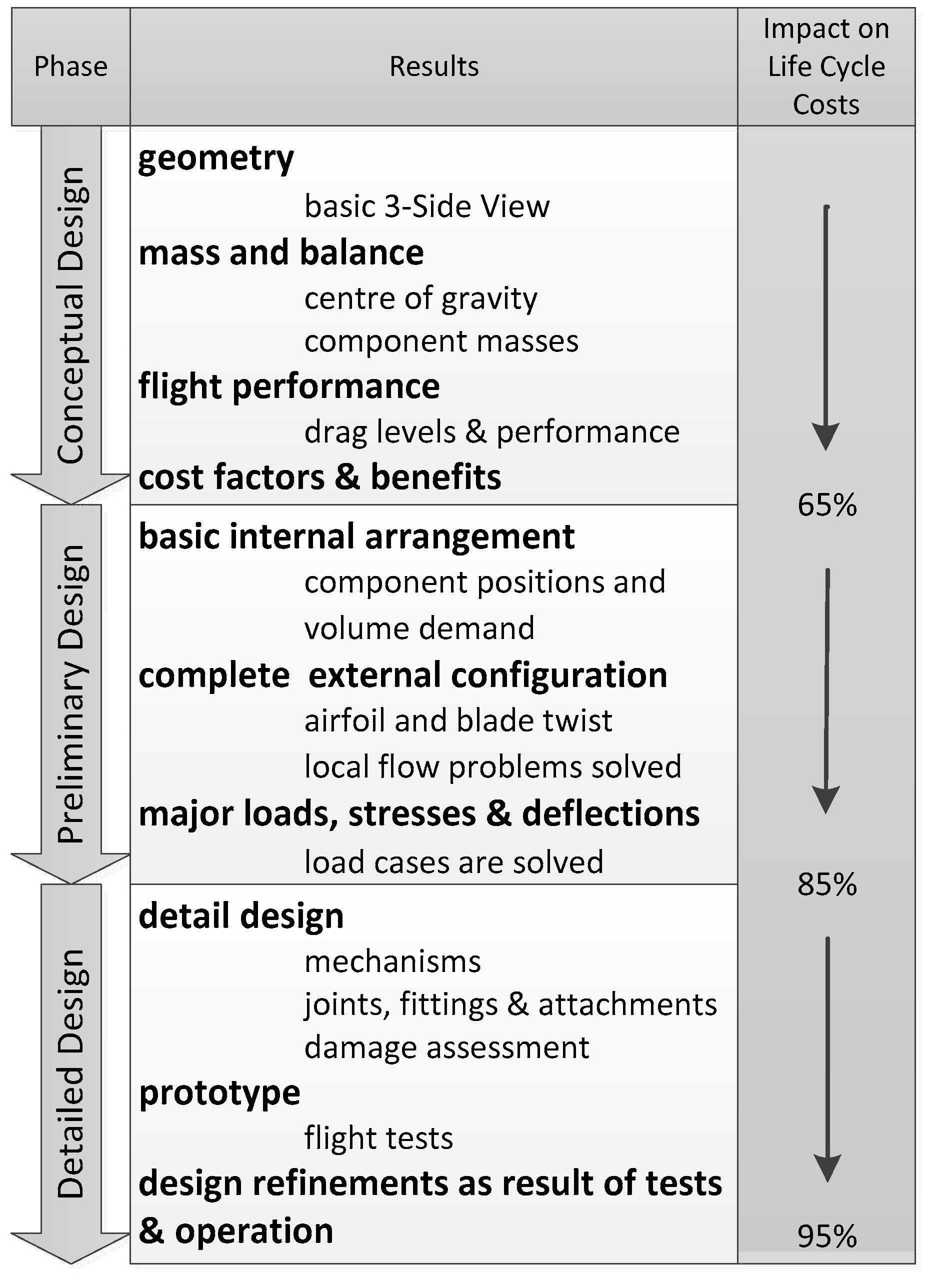
1.4. Design Theory

In the common literature the classical design process is divided into three phases. First the conceptual design, followed by the preliminary design, and finally the detailed design. Figure 1 outlines the design phases with the usual wording used for instance by Raymer [1] or Nicolai [10].

Here, the conceptual design delivers the external configuration of the vehicle determining its dimensions. The preliminary design delivers the internal configuration including component arrangement and the full description of the external shape. The detailed design is the most comprehensive phase. It includes the complete production drawings, ground testing, prototypes, etc. In some references these three phases are extended to five by a trend study at the beginning and a proposal status between the preliminary and detailed design phase, see Layton [12]. If these phases are not mentioned explicitly the trend study is conducted at the beginning of the conceptual design and the proposal status comes at the end of the preliminary design phase. The trend study gives first ideas about the economic sense of a new project and marks the first decision whether to start a project at all or to focus on a different one. The proposal is the last point to consider an execution of the project. Due to the complexity of the detailed design, there is no reasonable plan of terminating a project in the detailed design phase. Even though the small number of personnel working in the first phase compared to the second and in the second compared to the third, the results of the conceptual design already determine 65% of the life cycle costs of an aerial vehicle. By completing the preliminary design the grade of definition reaches 85% of the life cycle costs, see Roskam [11]. In traditional design approaches the design is frozen after completing each phase. New computational design methods featuring strongly networked tools allow switching between the first two phases. The working area of IRIS is the conceptual and partly the preliminary design with the ability to link the two design phases. Similar to the DLR design research on fixed-wing aircraft, presented by Liersch [13], the features of a distributed computation and a universal data model for harmonization and exchange are considered. Such modular and flexible workflows have shown to be very appropriate in civil and military fixed-wing design studies (see Liersch and Huber [14]), but are still not state of the art in rotorcraft design. This design methodology is the overall objective in the development of IRIS.

2. Design Environment

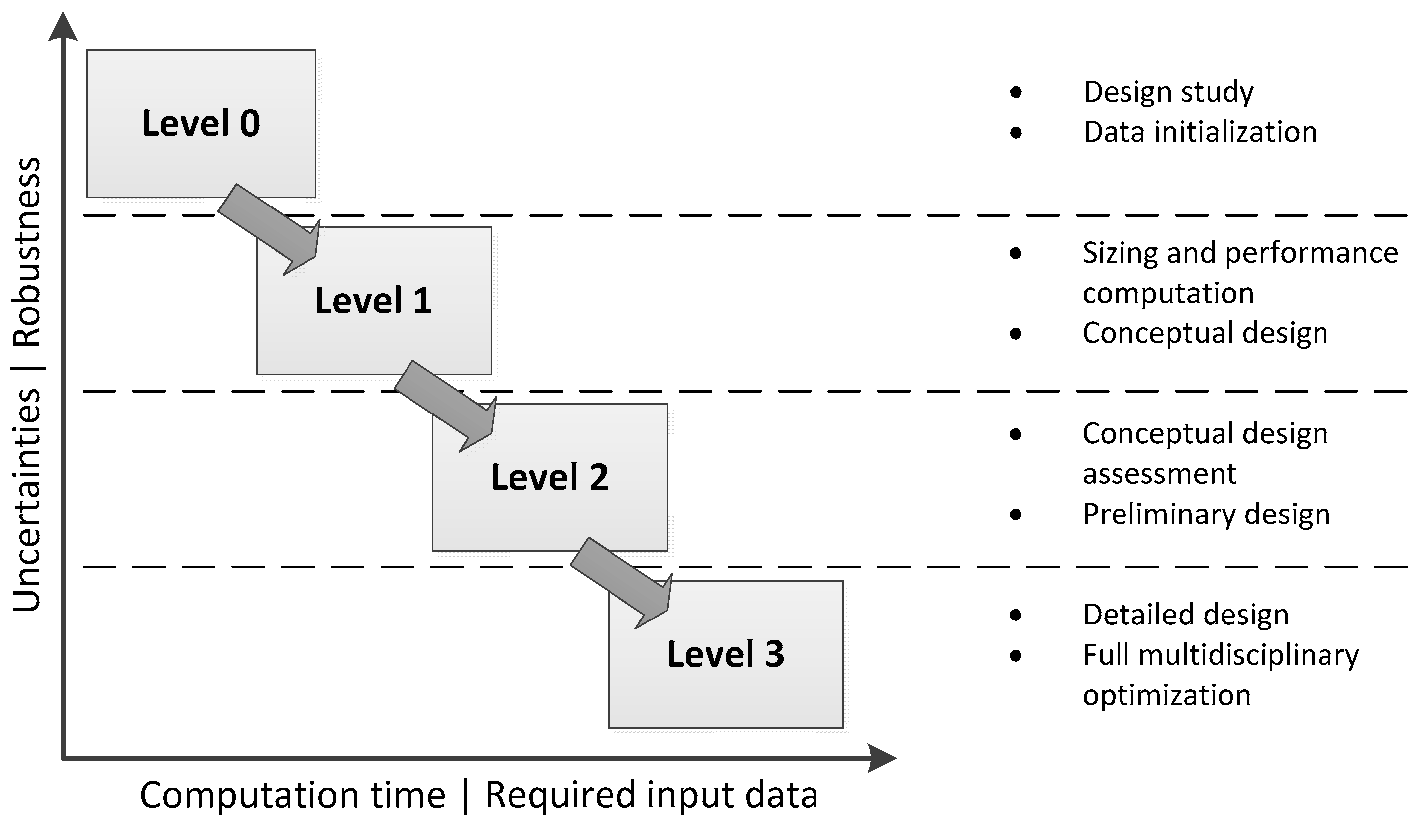
2.1. Tool Classification

The tools available differ from each other by different levels of accuracy, required input, robustness and computational time. The objective of a design process is to find a suitable arrangement of the tools in order to increase the amount of information with every step or loop and decrease the uncertainties. Therefore, the tools were divided into four groups, see Figure 2.

To evaluate individual tools the amount of input, output and the physical method have to be considered. One important characteristic is the ability to perform quick and iterative computations in a sizing loop.

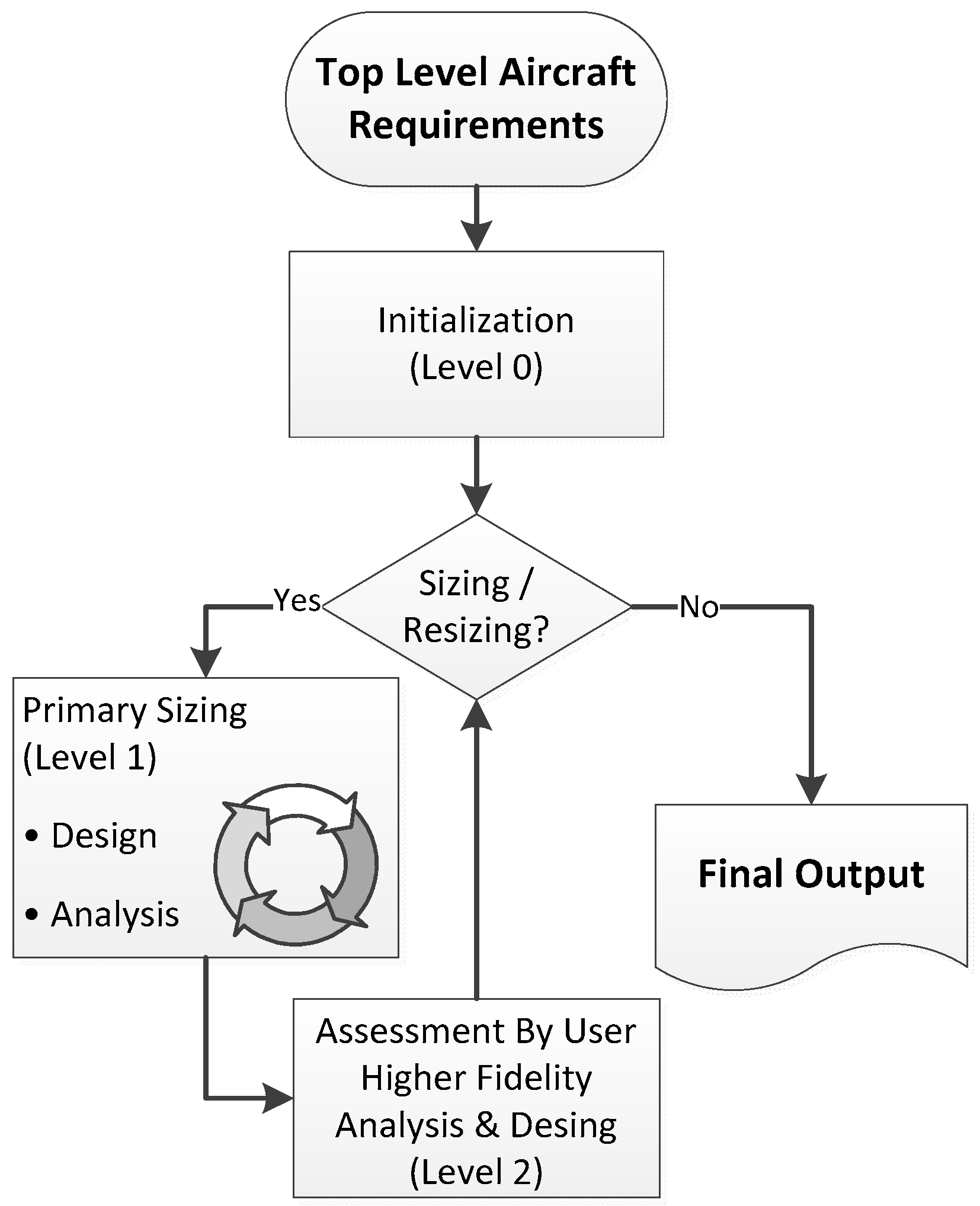
• Level 0 tools use statistical and simple physical models. No loops are performed on this level; therefore, the computation time is very low. These tools mark the first dataset based on the TLARs (Top Level Aircraft Requirements) and on knowledge-based data.
• Level 1 tools conduct the primary sizing. This procedure typically iterates the maximum take-off mass. The tools use physical models of low to medium complexity to achieve short computation time and hands-off calculation.
• Level 2 tools are characterized by a more sophisticated physical modeling. Their pre- and post-processing procedures can still be performed automatically, but the required computation time exceeds the boundaries of iterative sizing. Furthermore, a general diminishing of the robustness can be observed by increasing the accuracy of the methods. A good example is the consideration of higher order aerodynamic problems like interactions or separated flow. The possibility to see and check the plausibility of results has to be given.
• Level 3 tools have the highest fidelity and the most complex modeling. Pre- and post-processing procedures need additional input to solve necessary meshing tasks. In order to conduct full MDO (multidisciplinary design and optimization), secondary data has to be stored. The computation time is the highest. No level 3 tools are integrated into the presented design environment to date.

Dividing the several tools into different groups as presented in Figure 2 is a usual approach for building a design process, see Sinay [3] and Basset [6]. Every design approach features its individual data structure and strong points. It is difficult or even impossible to compare the tool classification, because the borders between the groups usually show strong differences from approach to approach, even for equal number of tool groups.

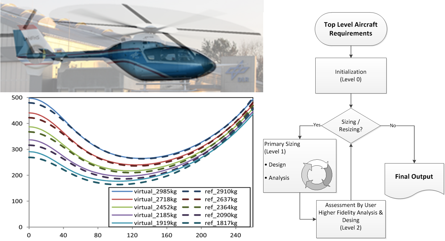
2.2. Process Architecture

According to the characteristics of the tool classification, the design process including level 0 to level 2 tools is arranged in three main sections, see Figure 3. The initialization is the first main section. Here the initial data set is computed by the level 0 tools. The second main section is the primary sizing. It is divided into a design section and an analysis section. The design section performs the sizing of the external configuration. The analysis section performs the recalculation of the initial mass fractions. Here a flight performance calculation delivering the required fuel mass and basic empty mass is computed by determining and summing up the individual component masses. The amount of data computed in the sizing loop must be sufficient to create a flight mechanic simulation model. The recalculation of the mass fractions delivers the updated maximum take-off mass and the new input for the next iteration. The convergence of the masses and external configuration derives a consistent design, which brings the mass of the vehicle, its outer dimensions and the required flight/transport performance into a plausible connection.

After sizing, the assessment and the higher fidelity computation are performed in the third main section with the level 2 tools. This may include a series of flight simulations in order to compute load cases for a finite element structural analysis (see Schwinn [15]). The results of these tools can be used to update the technology factors for the conceptual sizing loop. Changes and adaption of the design can be made. An updated data set with the need for resizing is fed back to the primary sizing loop.

2.3. Collaboration and Network

The features described above require a very sophisticated networking between the different computational tools which were usually hosted by individual specialists. Following the good experiences of DLR’s fixed-wing design summarized by Liersch [13], the approach of a distributed computation was also followed right from the beginning of the development of the rotorcraft sizing tool box. The network connection of the tools is ensured by the collaboration software RCE (Remote Component Environment) developed by DLR, see Bachmann [16] and Seider [17]. RCE is an open source software and the common resource for distributed processes in DLR projects. Tools can be stored on different servers and made available to design teams. The tools can be arranged in a graphical user interface.

The second important resource is a uniform data model to ensure the communication between the tools. The CPACS (Common Parametric Aircraft Configuration Schema) data model, see Böhnke [18] and Nagel [19], was originally developed as a communication language for fixed-wing design. CPACS has a strongly hierarchical XML structure and serves as a universal language for all integrated tools. The stored data include geometry, performance, requirements, component masses and more. The combination of CPACS and RCE has shown to be reliable (see Liersch [13]). Following the good experience with fixed-wing design CPACS was extended for rotorcraft design and implemented into the present rotorcraft design environment. The parametric description of fuselage, wings and stabilizers does not differ between the two types of aircraft. However, the description of the rotors, the mass breakdown, and flight performance requires some extensions. The further development of CPACS is an ongoing process for both fixed- and rotary-wing applications.

Since every tool uses the same CPACS data model for input and output, the process can easily be arranged. Adding and rearranging tools becomes an easy task of drag and drop and wiring the tools.

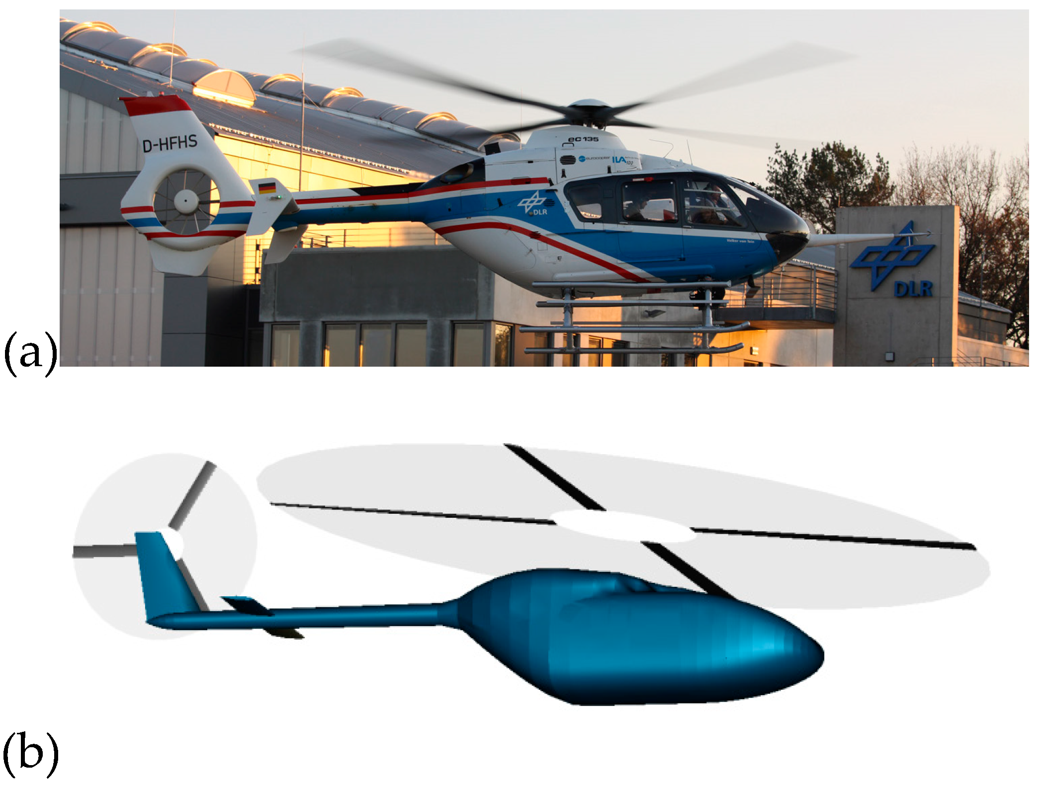
2.4. Implementation of Flight Simulation Tool

As mentioned above the ability to perform flight mechanic simulations inside the primary sizing loop determines the amount of data which has to be computed by the initialization main section and the design section. For the flight simulation and performance calculation in this design environment HOST (Helicopter Overall Simulation Tool) is used. HOST was originally designed by Airbus Helicopters (at that time Eurocopter) in the 1990s, see Benoit [20]. Its three main functions are trim calculations, time domain simulations and the calculation of linear equivalent systems.

As part of the level 1 tools the trim function is used to conduct the flight performance calculation. The flight performance calculation is part of the fuel estimation loop and is carried out in batch mode. Within this tool the pre- and post-processing procedures have to work automatically. Different shell and Python scripts are used for pre- and post-processing and for the generation of a flight mechanical model. After the calculation of the trim points the results are extracted from the simulation environment and stored in the design environment.

3. Initialization of First Data

3.1. Requirements

Generating the first data requires reading the requirements and generating the first configuration derived from those. These computations are very simple and straightforward. This computational group is assigned to level 0. The requirements usually are divided into three groups.

• The technical requirements determine the boundaries and demands for the external configuration. They describe and, if necessary, extrapolate the state of the art related to the specific design.
• The mission requirements give information about the use of the rotorcraft, which is at minimum the triplet of range, payload and flight speed.
• The performance requirements describe the flight conditions of the design mission profile and define the flight envelope.

Several approaches were conducted to find the minimum required TLARs for which the design process can be expected to generate reasonable output. This led to the question how much information could be derived from statistical regression and knowledge-based parametrization and what would be the fuzziness of the configuration with respect to the intended use of the rotorcraft. Five parameters listed in

Table 1. Minimum TLARs to start the process.

Name	Type of Parameter	Unit
Specific mission mass	real	kg
Cruise speed	real	m/s
Range	real	m
Number of main rotor blades	integer	-
Main rotor arrangement	text	-

have been found to be the minimum TLARs to initialize the process. The first three parameters are the triplet of the simplest flight performance. They determine how much useful mass shall be transported over what distance at which desired airspeed. The next two parameters determine the rotorcraft configuration. Besides the main rotor arrangement, specifying the number of main rotor blades has been found to be sensible. Additional requirements can be added in order to specify the results more clearly. This optional input may affect the sizing of the rotors with respect to a desired flight performance and the dimensions of the fuselage with respect to a required cabin layout.

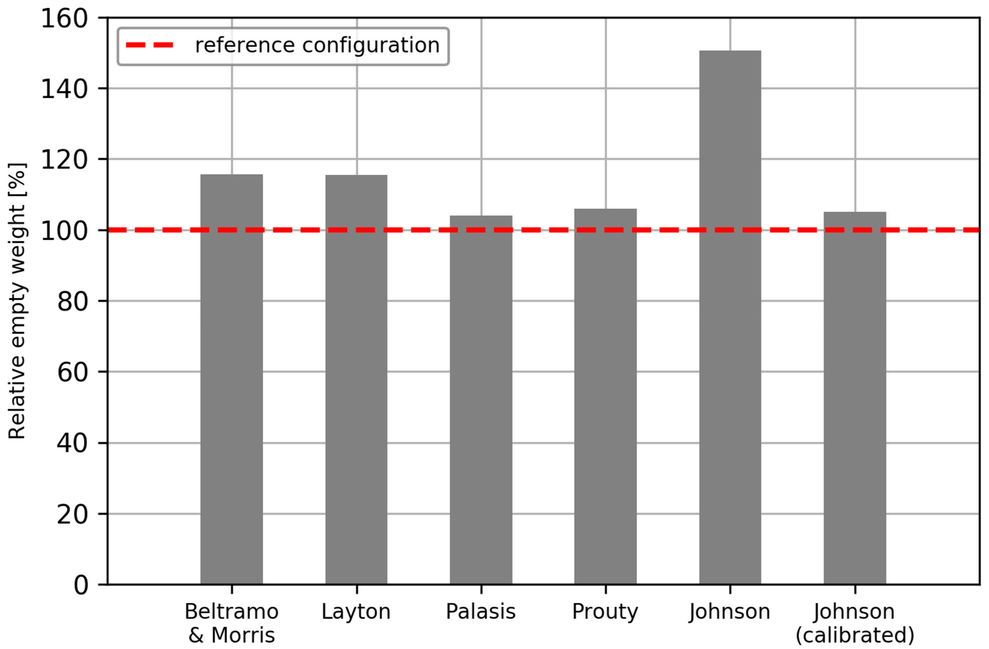
3.2. Mass Fractions

The empirical equations introduced in the following subsections to describe, e.g., the initial mass fractions or the rotor dimensions were derived from a statistical evaluation of 159 existing helicopter configurations.

The maximum take-off mass (MTOM) comprises the basic empty mass (BEM), the fuel mass (F) and the specific mission mass (SMM) given in Equation (1). The specific mission mass, as the second part of the useable load besides the fuel, is the sum of the payload (P), the operators mass (OM) and the specific mission equipment mass (EQU), see Equation (2). The result for Equation (2) has to be defined by the requirements. Computing the fuel mass and basic empty mass to solve Equation (1) is the fundamental task of the conceptual design.

$$m_{MTOM}=m_{BEM}+m_F+m_{SMM}$$

(1)

$$m_{SMM}=m_P+m_{OM}+m_{EQU}$$

(2)

Experience shows a good relation between the maximum take-off mass and the basic empty mass. The specific mission mass and the fuel mass form the useable mass. The true problem for initialization is that mission scenarios for rotorcraft are much more specific for each design than for fixed-wing. It is obvious from Equation (1) that different ratios of specific mission mass and fuel mass are possible for one maximum take-off mass. This is the fundamental reason for iterative computations in a sizing loop. In order to start such a loop an initial configuration has to be derived. The estimation of $m_{BEM}$ and $m_F$ by Equations (3) and (4) is one possibility, considering an increasing amount of equipment in Equation (2) for configurations resulting in more than 5 tons of $m_{MTOM}$.

$$m_{BEM}=2.9 \mathrm{kg} {\left(\frac{m_{SMM}}{\mathrm{kg}}\right)}^{0.9275}$$

(3)

$$m_F=4.8 \mathrm{kg} {\left(\frac{m_{SMM}}{\mathrm{kg}}\right)}^{0.6925}$$

(4)

3.3. First Dimensions of the Rotors

The maximum take-off mass $m_{MTOM}$ is the basis for the sizing of the external configuration. Most important are design properties of the main rotor or rotors in particular radius $R_{MR}$, mean cord $c_{MR}$, number of blades per rotor $N_{bl,MR}$ and tip speed $v_{tip,MR}$ as well as the ambient density $\mathsf{\rho }$. Vital parameters are the thrust coefficient $C_T$ and the rotor solidity $\mathsf{\sigma }$ given by Equations (5) and (6).

$$C_T=\frac{m_{MTOM}g}{\mathsf{\rho } {v_{tip,MR}}^2 \mathsf{\pi } {R_{MR}}^2}$$

(5)

$${\mathsf{\sigma }}_{MR}=\frac{N_{bl} c_{MR}}{\mathsf{\pi } R_{MR}}$$

(6)

The specific blade loading describes the non-dimensional thrust per blade and given by Equation (7). Values $C_T/\sigma \ge 0.12$ indicate first flow separations somewhere on the rotor disc (see van der Wall [21]).

$${\left(\frac{C_T}{\mathsf{\sigma }}\right)}_{MR}=\frac{m_{MTOM} g}{\mathsf{\rho } {v_{tip}}^2 N_{bl} c_{MR} R_{MR}}$$

(7)

Reasonable empirical approaches should not violate the aerodynamic boundaries of rotors. Suitable statistical values for the main rotor radius and solidity are given by Equations (8) and (9). For configurations with two main rotors a simple lift sharing can be applied adapting the input mass.

$$R_{MR}=0.226 \mathrm{m} {\left(\frac{m_{MTOM}}{\mathrm{kg}}\right)}^{0.392}$$

(8)

$${\mathsf{\sigma }}_{MR}=0.012 {\left(\frac{m_{MTOM}}{\mathrm{kg}}\right)}^{0.221}$$

(9)

Figure 4 shows the results of Equations (8) to (9) for a single main rotor. Density equals ground conditions with 1.225 kg/m³ and the tip speed was set to 210 m/s.

The thrust corresponds to hover with $m_{MTOM}$. The graphs show rotor radius as well as solidity increasing with $m_{MTOM}$. The resulting blade loading is slightly decreasing from 0.091 to 0.09 within reasonable values. In addition to Equations (8) and (9), the Equations (10) and (11) define the radius and solidity of a tail rotor.

$$R_{TR}=0.032 \mathrm{m} {\left(\frac{m_{MTOM}}{\mathrm{kg}}\right)}^{0.438}$$

(10)

$${\mathsf{\sigma }}_{TR}=0.018 {\left(\frac{m_{MTOM}}{\mathrm{kg}}\right)}^{0.241}$$

(11)

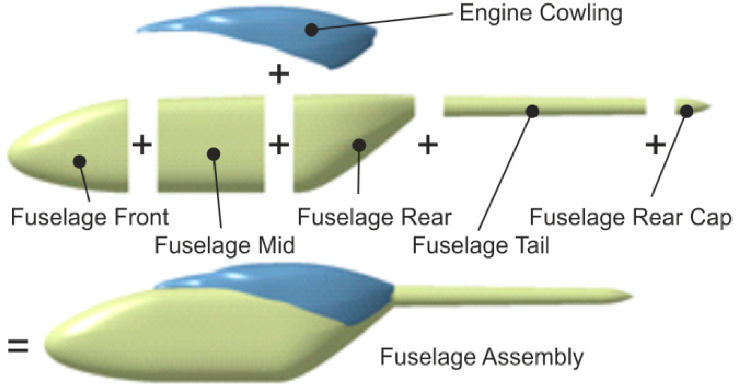
3.4. Fuselage Dimensions and Geometry Generation

With the evaluation of the TLARs a first sizing of the fuselage is performed in order to determine the dimensions of every fuselage part. The individual parts of the overall fuselage are shown in Figure 5. Basically, the fuselage comprises the body, the engine cowling and the tail boom. The body is parted into “Fuselage Front”, “Fuselage Mid” and “Fuselage Rear”. The front consists of the cockpit, the avionics and optionally a retractable nose gear. The “Fuselage Mid” part holds the cabin volume and the main landing gear if desired. The “Fuselage Rear” part can have doors, a stern ramp or a cargo hold.

If a tail boom is required, it consists of the “Fuselage Tail” and the “Fuselage Rear Cap”. The sizing starts with the cross section of the fuselage. The cross section has to consider the cabin dimensions plus additional space for structure, systems, and fuel tank. The lengths of the front and rear parts are related to the fuselage height. The length of the tail boom is defined by the position of the tail rotor and the stabilizers. The fuselage body including front, mid and rear part can be sized by using quantity equations for each dimension as functions of the payload mass. More precise results are obtained by giving additional inputs as shown in

Table 2. Optional requirements for cabin and fuselage.

Name	Type of Parameter	Unit
cabin height	continuous	m
cabin width	continuous	m
cabin length	continuous	m
cargo hold payload fraction	continuous	-

.

In addition to height, width and length of the cabin the cargo hold payload fraction gives the share of the payload, which is stored in an optional cargo hold, extending into the “Fuselage Rear” part according to Figure 5. Cargo hold payload fraction and cabin dimensions can be added independently. The parametrization of the fuselage parts is the basis for generating a 3D model.

A complex geometry generation by Kunze [22] is coupled with the commercial software CATIA V5, see the four examples given by Figure 6. Different templates for every fuselage part are saved. The templates for every part can be modified to nearly any arbitrary shape in order to conduct scaling from existing configurations or completely new ones.

Figure 6d shows an example for the arrangement of wings and propellers including a long rear part in order to minimize separation drag on the fuselage during high speed cruise. The surface model, as the basis for aerodynamic and structural computations, is saved in the CPACS file.

3.5. Calculation of Aerodynamic Coefficients

As mentioned in Section 2 the flight simulation tool HOST was implemented into the sizing loop to conduct the trim and performance calculations. To perform the complete trim an extended knowledge of the aerodynamic properties of the fuselage is essential. The algorithm inside HOST needs three force and three moment coefficients. The first option to compute the aerodynamic coefficients of the fuselage is by applying a panel method on the generated surface model described above. In the present approach a linearized 3D panel method is harmonized with the CPACS data model, see Kunze [22]. This tool is based on the commercial calculation tool VSAERO, see Maskew [23]. The code applies potential flow theory by modelling inviscid and incompressible flow. If desired, compressibility corrections can be applied. To account for the viscous drag, the approach is extended by an integral boundary layer formulation including a prediction of flow separation with an estimation of the pressure in the area behind the separation line. Figure 7 shows the streamlines on the surface of a scalable 3D model. The colorized streamlines show the estimated transition in the areas where the color changes from green to red. The streamlines end on the estimated separation line. Experience has shown that the prediction of the separation line gets coarser with increasing area of separation typically in connection with a blunt fuselage body. Here the shape of the area of separated flow sometimes does not deliver reasonable results. Reducing these errors and increasing accuracy is still part of further development of the panel code.

The results of this aerodynamic computation only take the clean surface of the fuselage into account. In order to cover further components like the rotor hub, landing gear, antennas or other attachments, a correction of the coefficients by handbook methods is required. Estimated drag areas for the rotor hub and the landing gear were derived from the investigation presented by Keys [24]. A further method of modelling the drag of the rotor hub is given by Stepniewski [25], where the rotor is divided into simple individual components for which drag areas are determined individually. For a rotor hub it is divided into blade shank, blade connection, bearing and middle section. The corresponding drag areas of the individual components are placed on the location of impact on the fuselage. All force and moment coefficients are corrected. For instance, the major impact of the hub drag is not only an increase of the force coefficient for the longitudinal axis; it also results in an apparent increase of the pitching moment.

4. Conceptual Sizing

4.1. Primary Sizing Loop

All subsequent level 1 tools are working iteratively. Here the sizing tasks and the analysis tasks, comprising the flight performance calculation and the basic empty mass estimation, are run successively. A typical convergence criterion for the maximum take-off mass is 0.5% relative deviation. Until convergence is obtained the process works hands off, including the generation of the flight mechanics model and calculation by HOST.

4.2. Sizing Tasks

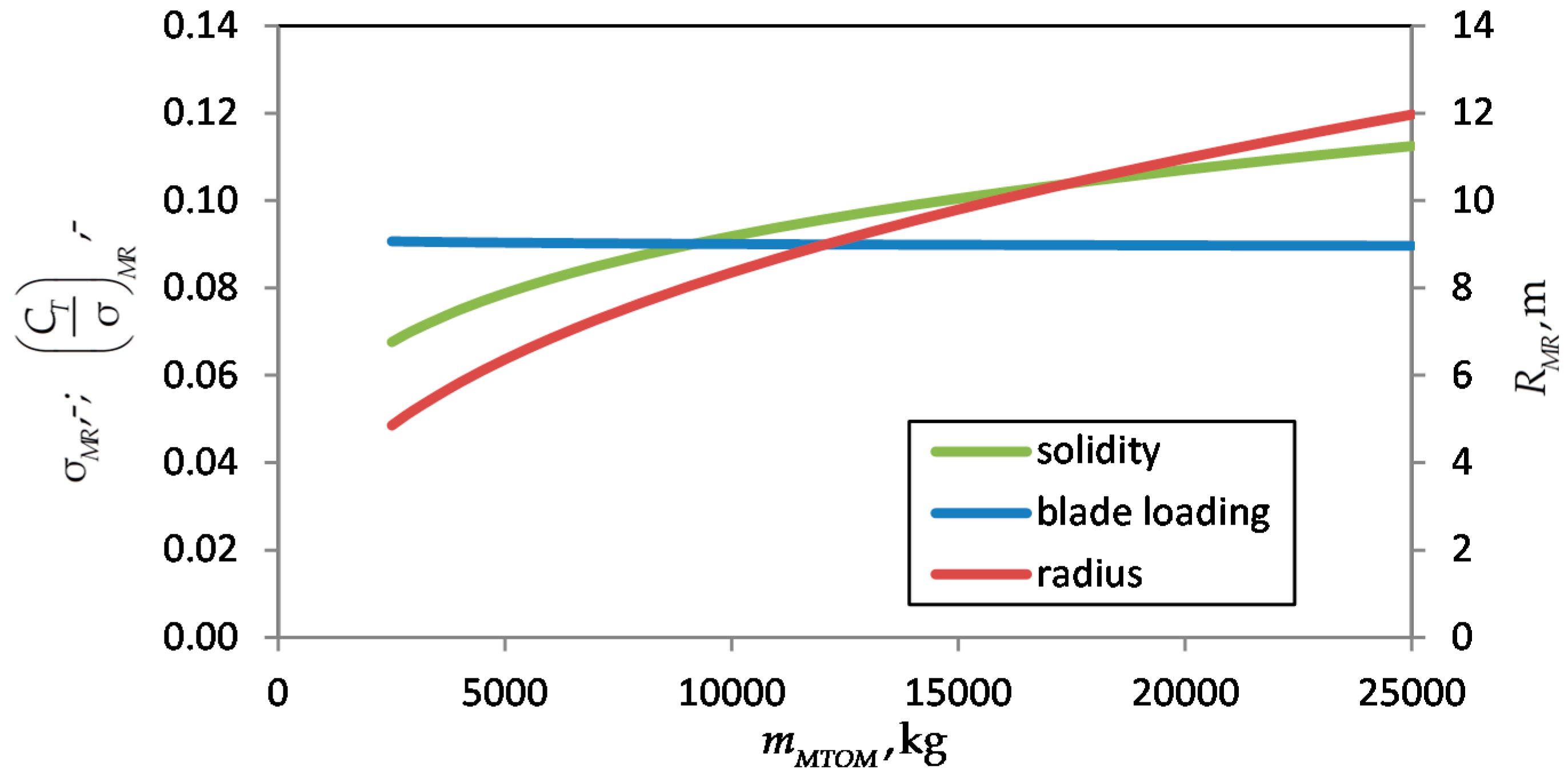
4.2.1. Rotor Sizing

There are different modes for the sizing of the main rotor(s) inside the primary loop which extend the level 0 sizing. Some of these modes can be combined with each other in order to meet with different sets of design parameters. The following features are covered for the sizing of the main rotor disc:

• Sizing with regression curves according to Equations (8) and (9).
• Sizing with a specified disc loading $DL=m_{MTOM}g/\pi {R_{MR}}^2$.
• Sizing with a specified blade loading in connection with different combinations of flight altitude and ambient temperature.
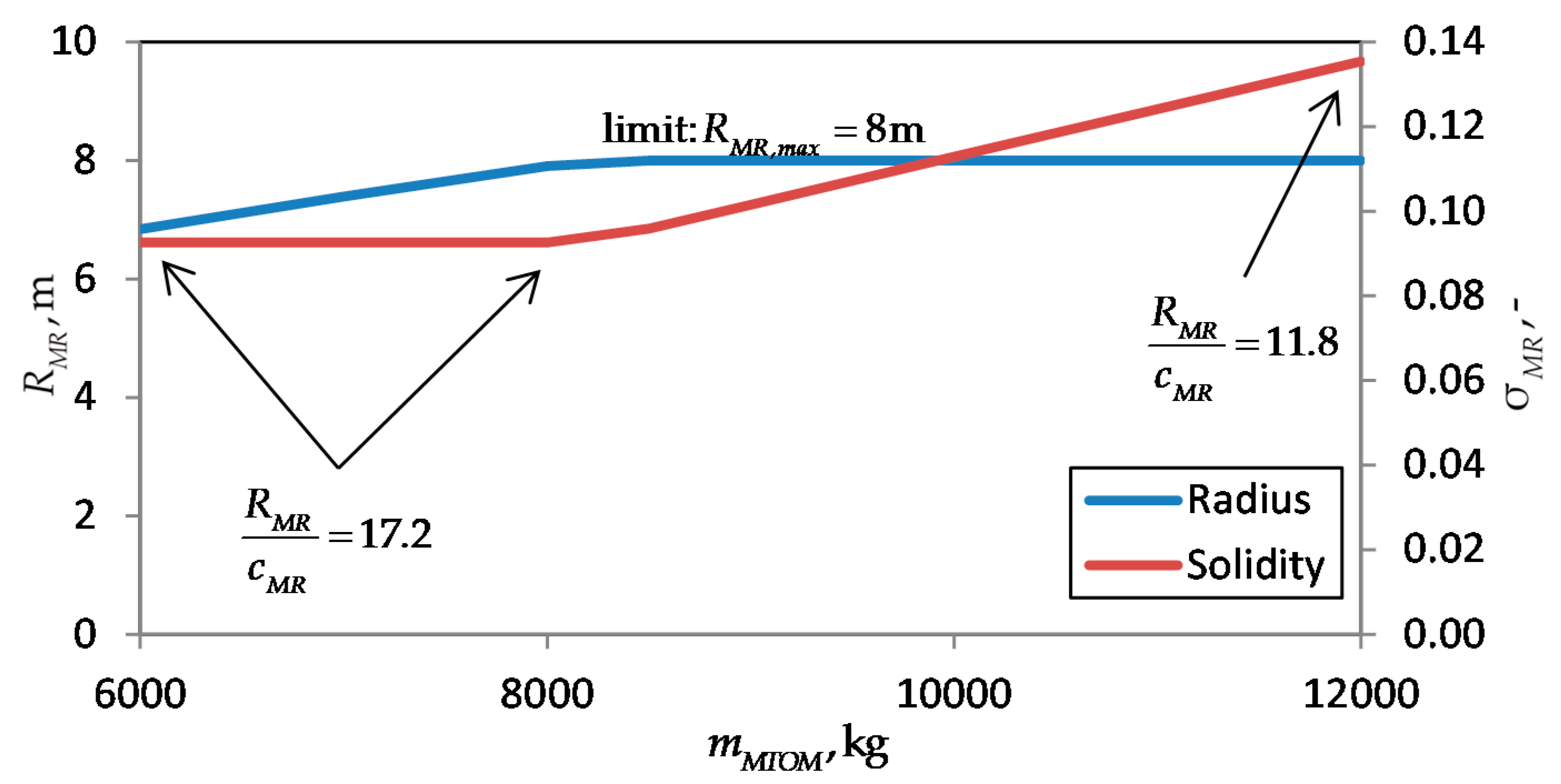
• Setting a boundary for a maximum allowed rotor radius.
• Setting a constant rotor radius and sizing the rotor solidity (constant blade loading with a variable disc loading)

A typical design approach explains the use of these modes at the following example. Assume a disc loading of 400 N/m² is given which may be the result from an assessment of the requirements and further optimization. Assume as well due to requirements for ship deck landing and hangars the maximum rotor radius maybe limited to 8 m. With respect to fast forward flight and maneuverability a suitable blade loading of 0.08 is chosen for hovering with $m_{MTOM}$ at zero altitude ISA (International Standard Atmosphere), based on previous design experiences. Figure 8 shows the radius and solidity for $m_{MTOM}$ from 6 tons to 12 tons. The single main rotor has five blades and a tip speed of 210 m/s.

With increasing take-off mass the rotor radius is increasing as well, keeping the disc loading constant. For constant thrust coefficient and a required blade loading the solidity is constant as well until the maximum radius of 8 m is reached. Now with increasing disc loading, the solidity has to be increased to meet with the blade loading requirement of 0.08. Here the aspect ratio of the blades decreases from 17.2 to 11.8. The number of blades should be reconsidered.

Beyond these analytical approaches, a knowledge-based optimization of the blade plan form as well as an optimization of the blade twist can be conducted (see Krenik [26]). An optional twist optimization minimizes the total power for a desired flight condition. A flight performance calculation requires the aerodynamic properties of the fuselage; hence, the computation of the fuselage aerodynamics and the generation of the geometry has to be carried out in a previous step.

One important parameter of aeromechanic similarity is the Lock number γ_MR which describes the ratio of aerodynamic moment to inertia moment of a rotor blade, as defined in Equation (12). To meet with the properties of a specific rotor technology it is functional to choose the Lock number as a design parameter. Equation (12) is solved for the flapping moment of inertia. Calculating the flapping moment of inertia J_β from the design Lock number and the present blade dimensions yields reasonable input for the later trim and performance calculation.

$${\mathsf{\gamma }}_{MR}=\frac{\mathsf{\rho }\cdot C_{l\mathsf{\alpha }}\cdot c_{MR}\cdot {R_{MR}}^4}{J_{\mathsf{\beta }}}\hspace{1em}\Rightarrow \hspace{1em}{J}_{\mathsf{\beta }}=\frac{\mathsf{\rho }\cdot C_{l\mathsf{\alpha }}\cdot c_{MR}\cdot {R_{MR}}^4}{{\mathsf{\gamma }}_{MR}}$$

(12)

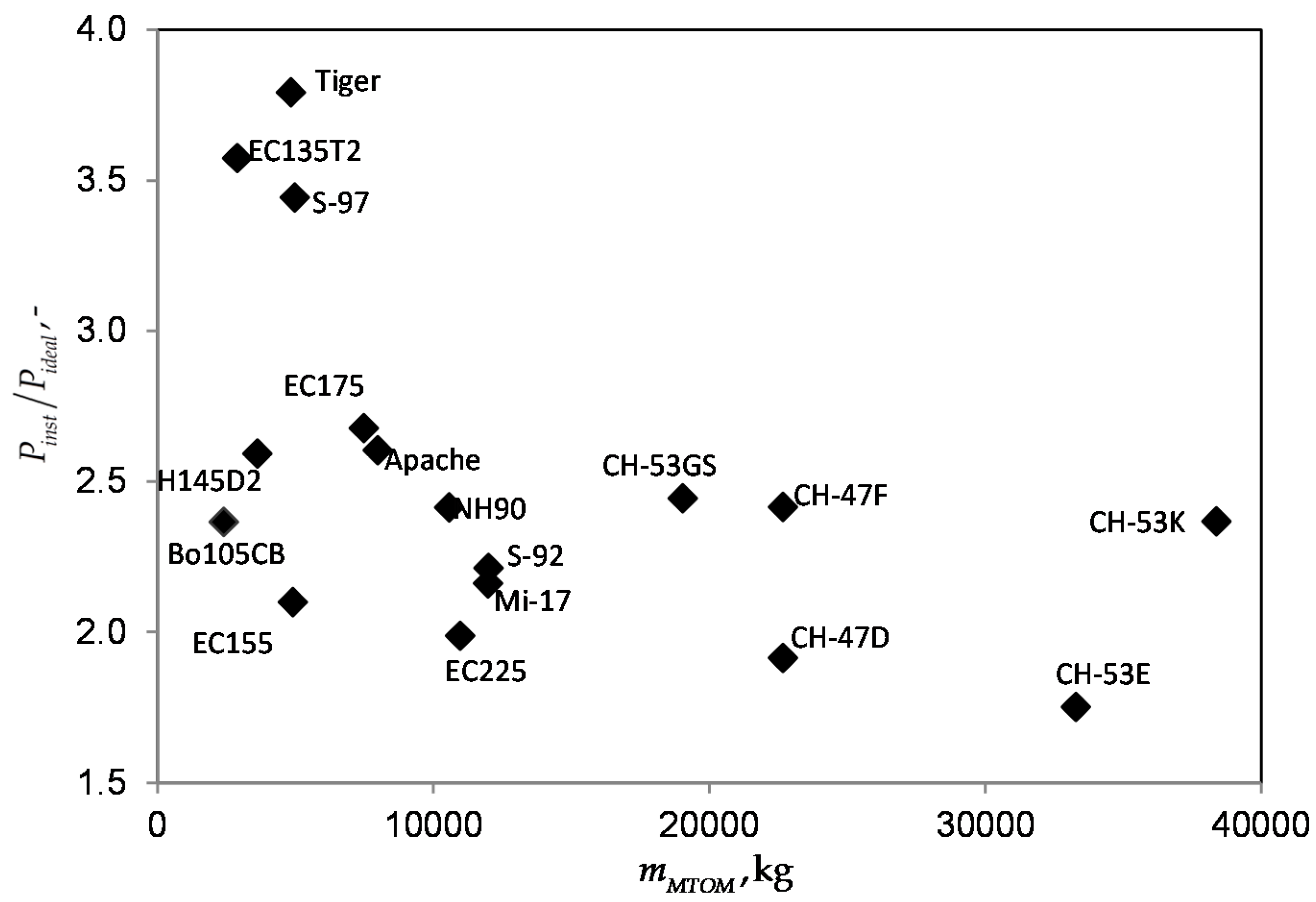
4.2.2. Installed Power

The total installed power of the engines is not only the power required to accomplish the mission. It also considers special performance requirements, such as for example hot and high flight conditions or the one engine inoperative state (OEI). A semi empirical approach showed to be very functional for the estimation of the installed power inside the sizing loop with varying disc area and maximum take-off mass. The ratio of the installed and ideal induced power is given with Equation (13). Figure 9 shows some typical values for existing helicopters considering ISA ground condition for the density $\mathsf{\rho }$.

$$\frac{P_{inst}}{P_{ideal}}=\frac{P_{inst}}{\sqrt{\frac{{\left(m_{MTOM}\cdot g\right)}^3}{2\cdot \mathsf{\rho }\cdot \mathsf{\pi }\cdot {R_{MR}}^2}}}$$

(13)

The installed power includes the 30 sec emergency power in case one engine is inoperative. The take-off and maximum continuous power ratings are lower. Most values of $P_{inst}/P_{ideal}$ range from 1.7 to 2.7 to fulfill the performance requirements with modern configurations around 2.4. The S-97 (3.44) is a compound configuration with increased flight speed and higher performance. Special requirements by operators like emergency cases for the EC135 (3.57) and survivability aspects for the Tiger (3.79) are above of this range. Considering such special configurations and boundaries the design parameters might need to be adapted.

4.2.3. Geometry Adaption

Fuselage configurations for contemporary and near future design studies differ from each other by the use of a tail boom, see for example Figure 6a,b for tail boom configurations in contrast to Figure 6c, the tandem configuration. For the standard and coaxial configuration, the cabin volume will be constant during the sizing. The variation of the rotor radius is taken into account by adjusting the length of the tail boom. For the tandem configuration a maximum overlapping ratio has to be taken into account. For instance, the overlapping of the CH-47 is 2/3 of the rotor radius. If the overlapping approaches the allowed minimum and an even larger rotor radius is required, than the mid-section of the fuselage has to be extended. The result is an increased cabin volume, larger than the required volume (see Figure 6c) and accompanied by increased mass.

4.2.4. Aerodynamic Coefficient

The scaling of the aerodynamic properties is conducted by the reference area and reference length. For the fuselage, reference area and reference length are typically given by the main rotor area and rotor radius. For wings and stabilizers, the lifting surface area and mean aerodynamic chord are allocated as reference. Since only minor changes of the fuselage geometry are conducted by iterating the maximum take-off mass, the impact on the aerodynamic coefficients of the fuselage in the level 1 computation is neglected. But a new computation of the fuselage coefficients after converged sizing and comparing with the previous coefficients may be reasonable.

4.3. Fuel Mass Estimation

4.3.1. Flight Mechanics Model Generation

Using all data calculated in the preceding modules and stored in the CPACS file, the required information is extracted to generate a simulation model. For example, necessary values are component positions, rotor dimensions, mass fractions, corrected aerodynamic coefficients of the fuselage including the rotor hub and landing gear and coefficients for the empennage. A simulation model consists of different submodels. Figure 10 shows the subdivision of a conventional main/tail rotor helicopter configuration into the different model files. With several different python scripts, the values needed are processed from the XML-paths of the CPACS file and written into the specific HOST model file. In this manner every submodel of the overall HOST model is generated.

The cell file describes the mass of the fuselage calculated during the sizing process, the position of the center of gravity (COG) and the inertia matrix.

The aero files of fuselage, horizontal and vertical stabilizer contain the translation and rotation positioning and the calculated and corrected fuselage coefficients from the preceding sizing task. Force and moment coefficients are tabulated as functions of the angle of attack and sideslip. The rotor files of main and tail rotor contain the general information, e.g., the positioning, number of blades of the rotor, mean chord and rotating speed.

The blade files describe the hub geometry with positions of prelead/lag, precone, lead/lag, flapping pitch and parameters for flapping stiffness and damping. Changes of these parameters are small from design study to design study and that is why empirical values are used. If necessary, they can be changed manually in the tool specific parametrization of the CPACS file or directly in the code.

Also, the blade geometry is defined in detail with chord and twist for every section and mass and inertia in the blade files. The swashplate files (in Figure 10 designated as platea) describe the dependencies of the commands (pedals, collective and cyclic control) to the pitch angles of the rotor blades. To synchronize the rotating directions and speeds of main/ tail rotor the motor file (in Figure 10 designated as moteur) is used. It does not represent a dynamic behavior of an engine. All models are merged in the general HOST file where the different movements, observations and interactions of the components are defined. For coaxial or tandem configurations, the simulation model contains different components like, for example, two main rotors without a tail rotor instead of one main rotor plus tail rotor.

All described model files are generated automatically during the sizing loop without the monitoring of the user. The execution of the HOST calculation is conducted in batch mode. At the end of the HOST module execution the results are post-processed and stored in the CPACS file. Python scripts are again used for this task. Typical outputs necessary for the flight performance calculation are the required power, the orientation of the rotorcraft and the command controls for the actual flight condition.

4.3.2. Calculation of Fuel Mass per Flight Segment

The computation of the fuel mass follows an iterative approach for every flight segment. This loop consists of the HOST calculation tool and a small script to adapt the fuel mass. At first the HOST calculation tool generates a simulation model as described before. HOST covers the trim and flight performance calculation at different flight conditions. Because all HOST calculations are executed in batch mode during the process, the generation of the trim condition file before every calculation is important. The parameters needed therein are: horizontal velocity (corresponds to the cruise velocity from the TLARs); first adopted orientation and control commands of the rotorcraft, and the current maximum take-off mass. The equilibrium law for the trim calculations is always six degrees of freedom calculation. Free parameters are four control commands (collective control, lateral control, longitudinal control and yaw control) and two fuselage orientations (pitch and roll angle). The four control commands are. The free orientations of the fuselage are. For the simplest mission requirement at least two trim points have to be used to calculate the actual range. These two conditions are at the beginning and at the end of a flight segment. With the required power the fuel consumption for every trim point is calculated. The total amount of fuel for the actual range is calculated by integrating the flight segment.

With the actual range $s_{RNG,actual}$ a small script adapts the initial fuel mass. First the difference $s_{RNG,dif}$ between actual and required range (segment range or at least overall range from the TLARs) is calculated. Then new fuel mass to minimize the difference is calculated with Equation (14).

$$m_{F,new}=m_F\frac{s_{RNG,dif}}{s_{RNG,actual}}$$

(14)

Convergence of the fuel mass is reached as soon as the difference between actual and required range is minimized with a change of the fuel mass less than 1%.

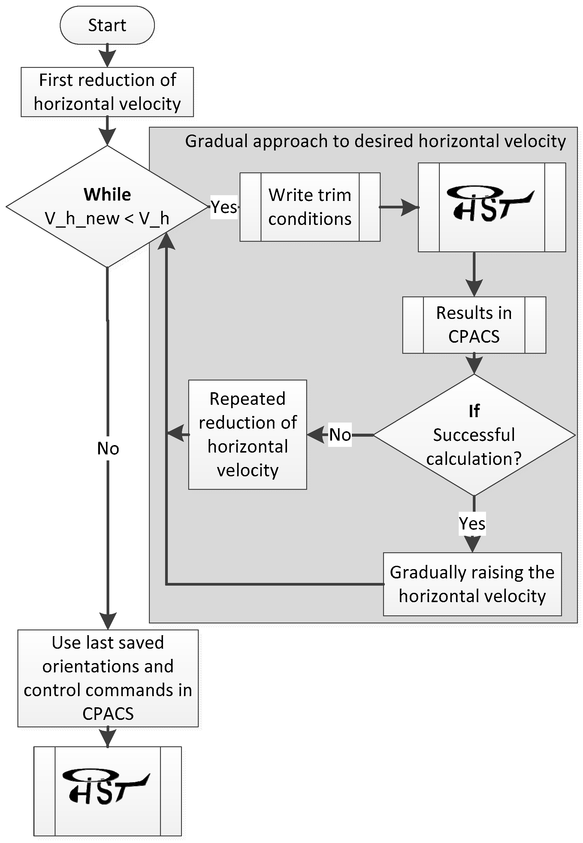
4.3.3. Special Considerations for Trim Points with High Velocities

For the design of contemporary and furthermore future rotorcraft flight conditions at the limits of the conventional rotor envelope have to be taken into account. At high flight speeds the aerodynamics of the rotor disc show increasing areas of nonlinear flow such as stall and transonic effects. These high-speed effects result in a worse convergence of the trim algorithms. Because no control commands or fuselage orientations are available as initial values before the first start of HOST, an immediate calculation of higher velocities can cause problems. There are different ways to solve such problems.

One way is to execute a trim sweep starting with hover and progressing up to the desired flight speed. Another way is to reduce the required velocity until the trim calculation obtains the equilibrium conditions and then gradually raising the velocity again until the required flight speed is reached. The results from every previous flight condition serve as the initial value for the next calculation.

This latter approach was chosen because many unnecessary calculations can be eliminated. Figure 11 shows the programmed process for the stepwise approach to a high velocity trim. The programmed process is a combination of python and shell scripts. Main part of the process is a while-loop which is executed until the velocity reaches the required end velocity $v_h$. It starts with a first reduction of the velocity to $v_{h,new}$. The amount of velocity that is reduced at this point is adjustable. At the moment 1% steps of the end velocity are used to have very small steps. This reduced velocity is the initial value for the while-loop.

First the trim condition file is written. The intermediate trim results for the six degrees of freedom are stored in CPACS file. The initial setup for these values is zero. Every time a calculation with reduced velocity was successful these values are updated and used as start values for the next calculation with an increased velocity. If the calculation is still unsuccessful, the velocity is reduced further. As soon as the velocities inside the while-loop approach the target velocity, after gradually increasing the velocity, the abort criteria is reached. A final trim calculation with the last calculated start values and final velocity is now executed delivering the final results for one trim point.

This approach is completely automatic and can be applied for every HOST calculation in the design environment to deal with flight conditions at higher velocities.

4.4. Component Mass Estimation

Mass estimation is an essential part in the conceptual design stage since the mass of the aircraft determines and influences directly and indirectly other design aspects, e.g., rotor, fuel, flight performance, airframe, etc. In general, at the early stage in the overall design process, the mass of components such as structure, systems, and propulsion can be estimated using a statistical approach that compares similar rotorcraft configurations. In addition to Equation (1) the basic empty mass can be extended by estimating and summing up the subcomponent masses (structure(struc), propulsion(propu), systems(syst)) and the operators (OM) items, as broken down in Equation (15).

$$m_{OEM}=m_{BEM}+m_{OM}=m_{struc}+m_{propu}+m_{syst}+m_{OM}$$

(15)

Therefore, statistical mass estimation methods have been integrated into the design process. Currently, the mass estimation according to the methods proposed by Beltramo and Morris [27], Palasis [28], Layton [12], Prouty [29], and the AFDD-models presented by Johnson [2] have been implemented. Johnson introduced the AFDD (U.S. Army Aeroflightdynamics Directorate) mass models that feature the highest grade of coupling of geometric and performance characteristics. Moreover, his methods provide the use of so-called technology factors that can be used to scale component masses with respect to their compositions. Figure 12 compares the implemented mass estimation methods using a Bo105 as reference configuration.

It can be observed that—except the AFDD models by Johnson—the earliest methods (Beltramo and Morris and Layton) feature a high deviation of slightly less than 20%. The methods of Palasis which are a mixture of the methods of Beltramo and Morris, and Layton, result in a very precise estimate. Prouty’s estimation is slightly higher than the one by Palasis but still very close to the real weight. The methods by Johnson show the highest deviation though being the latest method. The reason for this deviation is that for many systems (e.g., electrics, avionics, etc.) no equations are provided but only lower and upper limits specified, valid for medium weight helicopters. Linear interpolation for these systems may lead to unreasonable deviations. Therefore, it is recommended to use specific, fixed input weights which are often not yet established at early conceptual design level. Instead of applying fixed input weights the AFDD models were calibrated by using technology factors for all systems down to the subsystem level as done by Russell and Basset [7]. Since helicopter design is strongly driven by functionality, a statistical approach for those systems is merely too difficult to realize and should be handled by providing a fixed input mass (as available) to avoid large deviations. It can be observed that due to the calibration (last bar in Figure 12) the BEM drops significantly resulting in an adequate estimate close to the methods by Palasis and Prouty.

5. Example for Sizing Study

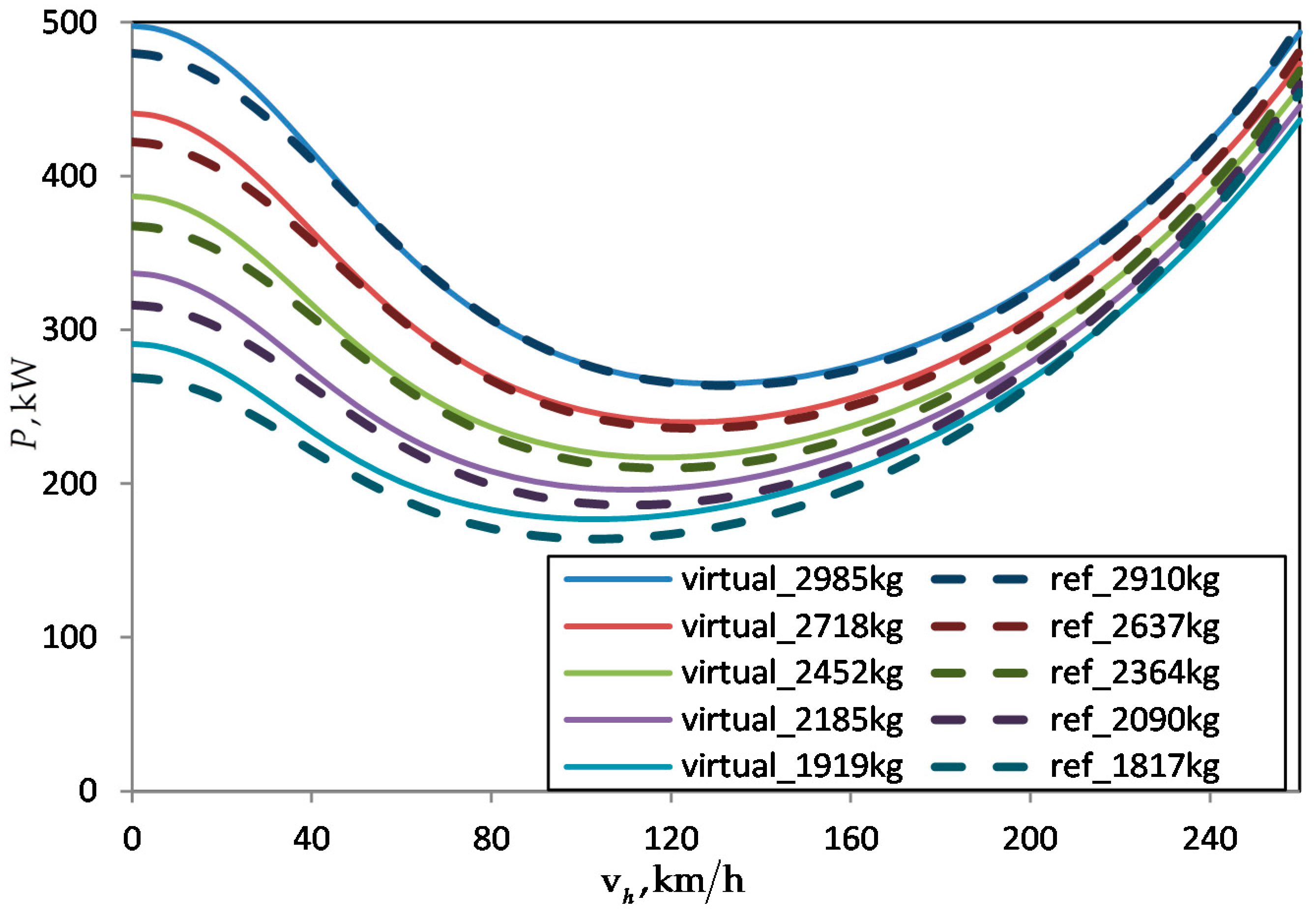
5.1. Evaluation by Short Design Study

DLR has gained extensive experience with its research helicopter ACT/FHS (Advanced Control Technology/Flying Helicopter Simulator). This is a highly modified variant of an EC135, a typical option for HEMS (Helicopter Emergency Medical Services) operations below 3 tons maximum take-off mass (see Figure 13a and Kaletka [30]). A validated HOST model for the ACT/FHS is available. Experience has shown that it is a good reference for a design study.

Table 3. Minimum TLARs identified for the ACT/FHS research helicopter.

Parameter	Value
Payload mass	809 kg
Cruise speed	65 m/s
Range	615 km
Number of main rotor blades	4
main rotor arrangement	standard

shows the minimum TLARs identified by DLR for the ACT/FHS.

The cabin volume was averaged to a cubic shape; reasonable requirements for the interior were derived and listed in

Table 4. Additional requirements for the cabin of an ACT/FHS like rotorcraft.

Parameter	Value
Cabin height	1.25 m
Cabin width	1.5 m
Cabin length	1.7 m
Cargo hold payload fraction	0.2

. Here only the room behind the two cockpit seats is considered.

Computation was started with the input from Table 3 and Table 4. Fuselage templates were chosen with a simplified shape of the ACT/FHS. Figure 13 compares the external configurations by a photograph of the ACT/FHS (a) with the 3D model (b) from the design output. For the present design study, a three-bladed tail rotor was chosen, since the complete scalable model of a Fenestron including collector, rotor, stator and diffuser is not implemented at the moment.

The resulting dimensions of the configuration are listed in

Table 5. Characteristic parameters of the reference configuration and the case study.

Parameter	ACT/FHS Reference	IRIS Virtual	Deviation
$m_{MTOM}, \mathrm{kg}$	2910	2985	2.58%
$m_{BEM}, \mathrm{kg}$	1544	1652	6.99%
$m_F, \mathrm{kg}$	557	524	−5.92%
$R_{MR}, \mathrm{m}$	5.10	5.20	1.90%
$c_{MR}, \mathrm{m}$	0.289	0.286	−1.04%
$l_{FUS}, \mathrm{m}$	10.21	9.92	−2.80%
$DL, \mathrm{N}/{\mathrm{m}}^2$	349	345	−1.22%
${\mathsf{\Omega }}_{MR}, \mathrm{rad}/\mathrm{s}$	41.4	40.40	−2.29%
${\mathsf{\sigma }}_{MR}, -$	0.072	0.070	−2.68%
$C_T/\mathsf{\sigma }, -$	0.089	0.091	2.38%

. The parameters mainly show a good agreement. The most significant divergences are recognized between the basic empty mass and the fuel mass. Obviously, these parameters are the main outputs of the conceptual sizing and therefore the sum of all uncertainties. Luckily for this case study these errors nearly cancel each other.

The useable mass, i.e., the sum of fuel and specific mission mass, of the virtual configuration is 1333 kg and 2.42% less the useable mass of the reference aircraft (1366 kg). In order to find reasonable trim masses for a comparison of the flight performance curves the ratio of the usable mass with respect to the flight mass was varied from 20%, to 100% in increasement of 20% for the virtual and the reference configuration. The sum of useable mass and basic empty mass resulted in slightly different flight masses as indicated in the legend of Figure 14 where the power required is shown for the ACT/FHS model of HOST (reference) and the virtual configuration.

The power required is the sum of the main rotor and the anti-torque power. Gear losses and systems power are not included in this graph. The solid lines represent the performance curves of the virtual configuration and the dashed lines represent the reference. Induced power and airfoil power are slightly higher for the virtual configuration. As seen in the labels of Figure 14 the flight masses of the virtual configuration are higher compared to the reference. The airfoils used for the sizing during the design study are NACA 23012 which have a worse lift/drag ratio then the airfoils actually used on the reference and show an increased airfoil drag in comparison to the original airfoils developed by Airbus.

On the other side the parasite drag of the virtual fuselage is a little bit lower since the aerodynamic computation of the fuselage does not take all attachments on the surface into account. This results in closing the gap between two required power curves of comparable useable load at higher flight speeds.

A breakdown of the basic empty mass is given in

Table 6. Breakdown of the component masses for the virtual configuration.

Mass Component	mcomp, kg
Rotor group	220
Engines	201
Transmission	23
Fuselage	266
Empennage	15
Landing gear	131
Nacelle	44
Air-condition & anti-icing	17
Auxiliary power	42
Avionics	133
Electrics	130
Flight controls	55
Fuel system	55
Furnishing	193
Hydraulics	15
Instruments	48
Load handling	65
Basic empty mass Σ =	1652

. The validation of the individual component masses is difficult because of the lack of access to reliable reference data. For instance, the mass of the transmission listed in Table 6 seems to be very low. However, summing up all components results in a basic empty mass 6.99% higher than the reference.

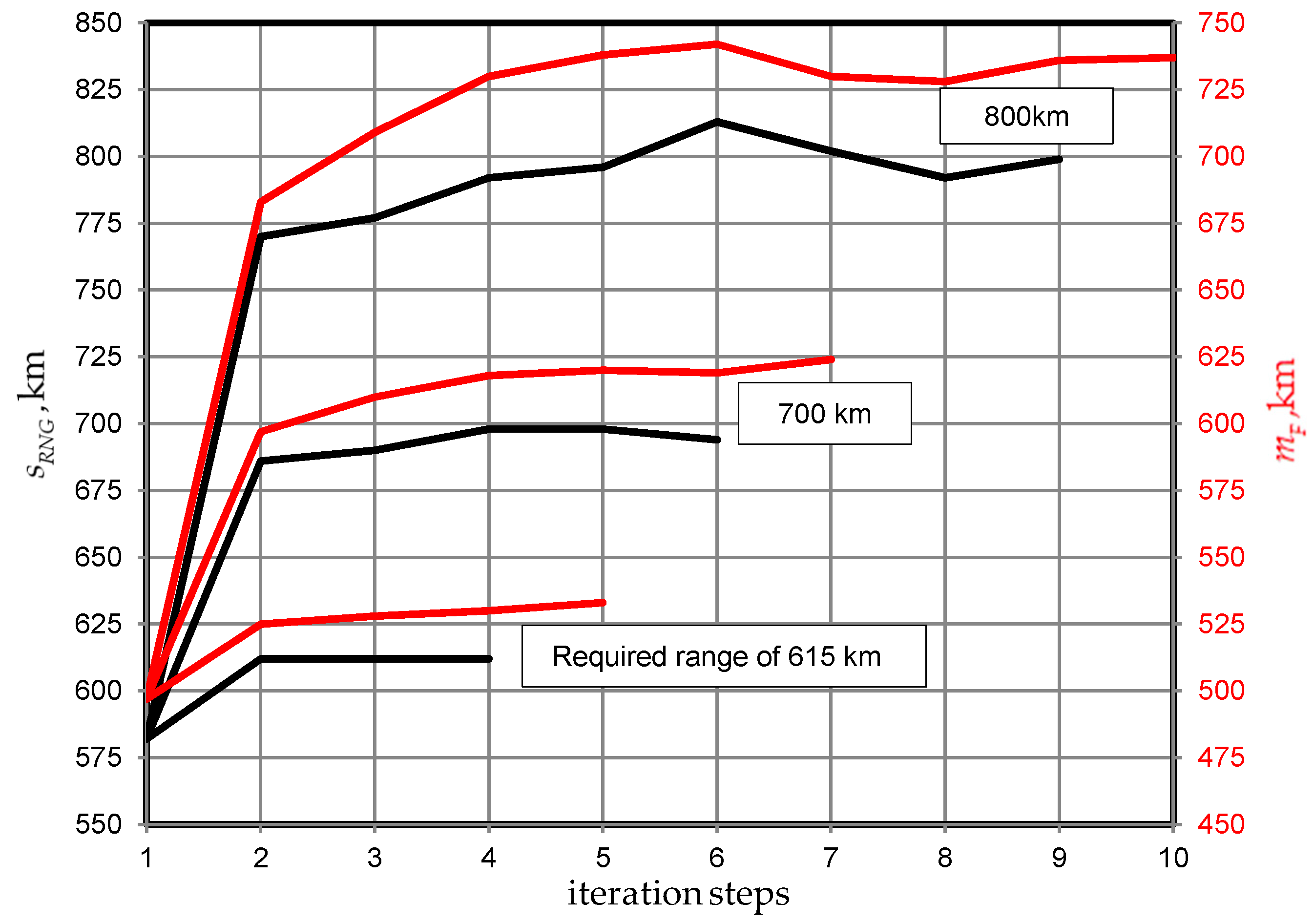
5.2. Variation of Flight Range

Three different flight ranges were chosen and the impact on the overall configuration was examined. The range for the first calculation was set to 615 km as specified in Table 3. For the second and third calculation, ranges of 700 km and 800 km were chosen, while all the other TLARs remain fixed. The resulting fuel masses corresponding to the three ranges are shown in Figure 15.

The results show the actual range (black) and fuel mass (red) versus the iteration steps during the fuel estimation loop. Only the last results point of the curves shows the fuel mass for the given range, indicating results have converged at this point. To cover up the range difference the fuel mass has to be increased. After the fuel calculation has ended the whole sizing loop continues and iterates until the maximum take-off mass converges. When the required range becomes larger more calculations are necessary to approach the range and finally converge the fuel mass.

The result of the calculation with a required range of 615 km shows a fast approach to the range and, after a first jump, a smooth increase of the fuel mass to convergence after four calculations. For a required range of 615 km the process ends with a fuel mass of 534 kg.

For a required range of 700 km the fuel mass converges after six calculations. The required range is reached after four calculations. The fuel mass changes afterwards are small and only wait to finish until the maximum take-off mass of the whole sizing loop converges.

That is why six calculations are carried out although the required range is reached after four calculations. At the end the calculation finishes with 624 kg fuel mass.

The results of the last calculation with a required range of 800 km in Figure 15 show a similar behavior resulting in a fuel mass of 737 kg. The general results, including the disk and blade loading, of the three different calculations are listed in

Table 7. Characteristic parameters of the reference and virtual configuration with 3 design ranges.

Parameter	ACT/FHS	615 km	700 km	800 km
$m_{MTOM}, \mathrm{kg}$	2910	2985	3069	3240
$m_{BEM}, \mathrm{kg}$	1544	1652	1635	1694
$m_F, \mathrm{kg}$	557	534	624	737
$R_{MR}, \mathrm{m}$	5.10	5.20	5.25	5.35
$c_{MR}, \mathrm{m}$	0.289	0.286	0.291	0.300
${\mathsf{\Omega }}_{MR}, \mathrm{rad}/\mathrm{s}$	41.35	40.40	40.03	39.23
$DL, \mathrm{N}/{\mathrm{m}}^2$	349	345	348	353
$C_T/\mathsf{\sigma }, -$	0.089	0.091	0.091	0.092

, together with the parameters of the reference helicopter.

It is seen that not only the fuel mass changes because of a variation of the required range. The higher fuel mass leads to an increased basic empty mass and a higher blade mass calculated by the mass estimation module, which results in a bigger maximum take-off mass at the end of the sizing loop. Also, the rotor sizing responds because of the higher disk loading for a higher required range, which results from a higher maximum take-off mass. The radius and mean chord increase to compensate the higher mass, too.

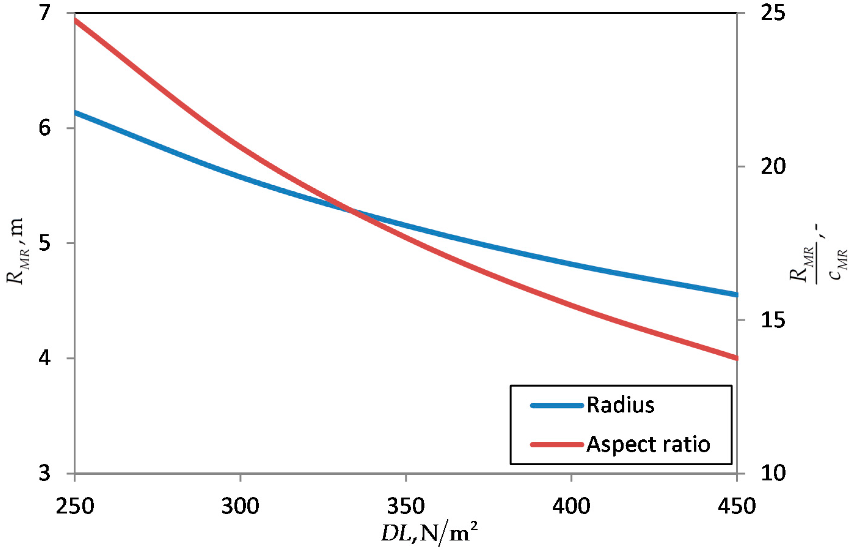
5.3. Variation of Design Parameters

The sensitivity of the tools is demonstrated with a further variation of the design parameters. Here a variation of the disc loading is conducted while keeping a constant blade loading. Table 5 shows values for the disc loading about $DL\approx 350 \mathrm{N}/{\mathrm{m}}^2$ and blade loadings around $C_T/\mathsf{\sigma }\approx 0.09$. The disc loading is now varied to four additional levels, two above and two beyond the baseline. The resulting mass contributions for $DL=250 \mathrm{N}/{\mathrm{m}}^2$ to $DL=450 \mathrm{N}/{\mathrm{m}}^2$ are shown in

Table 8. Primary mass contributions for a variation of the disc loading.

DL	250 N/m2	300 N/m2	350 N/m2	400 N/m2	450 N/m2
$m_{MTOM}, \mathrm{kg}$	3029	2999	2988	2987	2996
$m_{BEM}, \mathrm{kg}$	1718	1677	1653	1636	1629
$m_F, \mathrm{kg}$	502	513	526	541	558

.

The maximum take-off mass has a minimum between $DL=350 \mathrm{N}/{\mathrm{m}}^2$ and $DL=400 \mathrm{N}/{\mathrm{m}}^2$. It can be shown how the basic empty mass decreases with increasing disc loading, while the fuel mass increases. Figure 16 shows the rotor radius and blade aspect ratio over the disc loading.

For the baseline design the blade of the ACT/FHS has a radius of 5.1 m with an aspect ratio of 17.6. By increasing the disc loading the aspect ratio decreases from 24.8 to 13.8 resulting in a significantly increased blade mass with disc loadings below 350 N/m². The fuel mass is computed for a single flight segment of 615 km at 65 m/s flight speed resulting in a low induced power for the design point. Considering a certain hover efficiency, it seems a disc loading of more than 350 N/m² would lead to a strong increase of the required fuel mass at off-design flight conditions.

Another variation of design parameters is applied by including additional performance requirements for hot and high flight conditions. The most popular design criterion for hot and high operations is safe hovering out-of-ground effect at an altitude of 1830 m with a temperature of 35°C (the Army Hot Day: 6000 ft and 95 °F). Experience has shown that rotorcraft should not be operated with a blade loading of more than 0.11 to ensure take-off, hover and safe control in case of potential disturbances. This may lead to a $C_T/\mathsf{\sigma }\le 0.09$ at sea level depending on the resulting air density for the required condition.

The power available from the engines, due to one engine inoperative requirements resulting in a high installed power (see Figure 9), is considered to be sufficient. The mission requirements will not be affected. A comparison of the baseline configuration with the “hot & high” capable configuration is shown in

Table 9. Variation of the rotor design parameters for hot and high performance requirements.

Parameter	Baseline Vehicle	Hot & High Variation	Deviation
$m_{MTOM}, \mathrm{kg}$	2988	3061	2.43%
$m_{BEM}, \mathrm{kg}$	1653	1705	3.14%
$m_F, \mathrm{kg}$	526	547	3.96%
$R_{MR}, \mathrm{m}$	5.15	5.22	1.20%
$c_{MR}, \mathrm{m}$	0.291	0.322	10.51%
${\mathsf{\Omega }}_{MR}, \mathrm{rad}/\mathrm{s}$	40.7	40.3	−1.08%
${\mathsf{\sigma }}_{MR} , -$	0.072	0.079	9.20%
$C_T/\mathsf{\sigma }, -$	0.090	0.083	−8.60%
$m_{SMM}/m_{MTOM}, -$	0.27	0.26	−2.38%

. The most recognizable deviation is the increased mean chord and rotor solidity. The blade loading for ground conditions with maximum take-off mass drops from 0.09 to 0.083. The resulting rise of airfoil power causes an increase of required fuel and of the maximum take-off mass in connection with a higher basic empty mass.

6. Preliminary Design of the Fuselage Structure

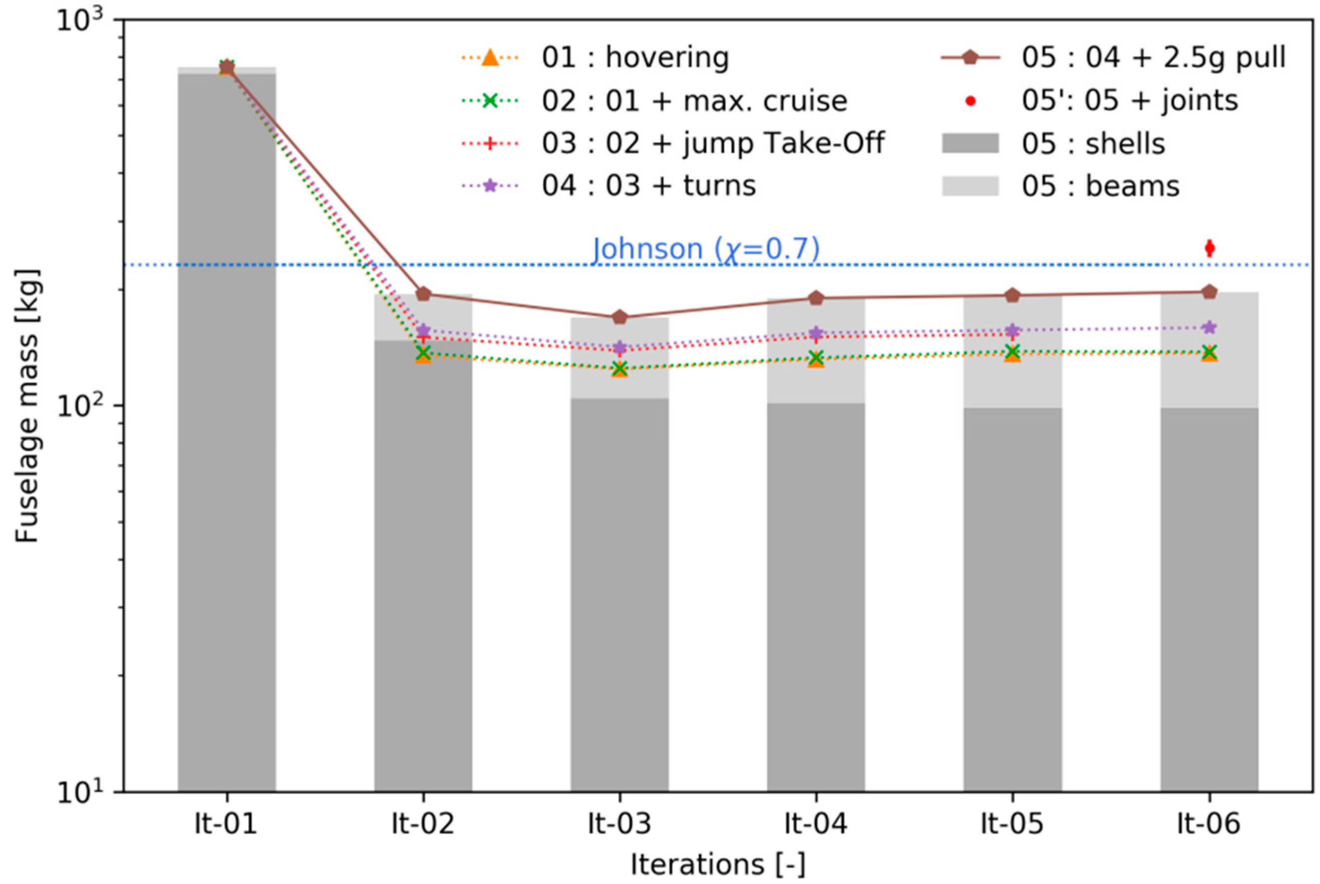
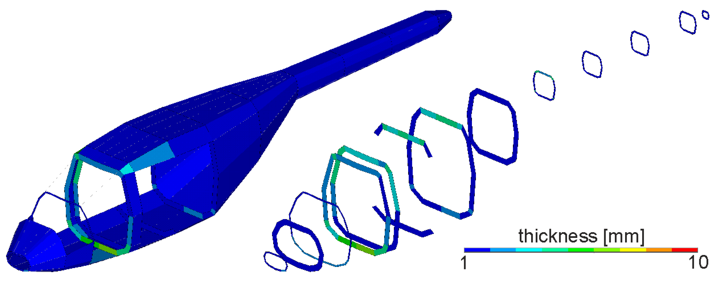
6.1. Computational Mass Estimation

As mentioned in Section 4.4, the conceptual design approach to estimate the fuselage mass depends on statistics and gives only a rough estimate. It often does not take into account specific performance requirements like flight maneuvers, or specific configurations, such as compound configurations that feature additional lifting surfaces.

Due to the continuously increasing computational power nowadays, a finite element (FE) analysis module was integrated into IRIS. This tool requires more input, than the conceptual design tools mentioned above. The computational time and the time required for the processing of input and output are also higher. Therefore, it is considered as Level 2 tool, representing preliminary design stage. Subsequently the model generation, the analysis, and an implemented sizing routine for static and quasi-static load cases will be introduced.

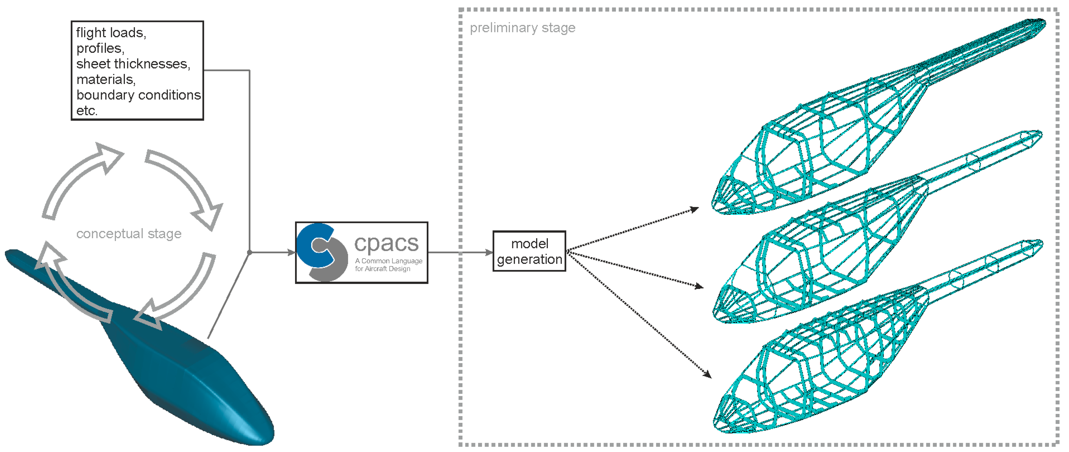
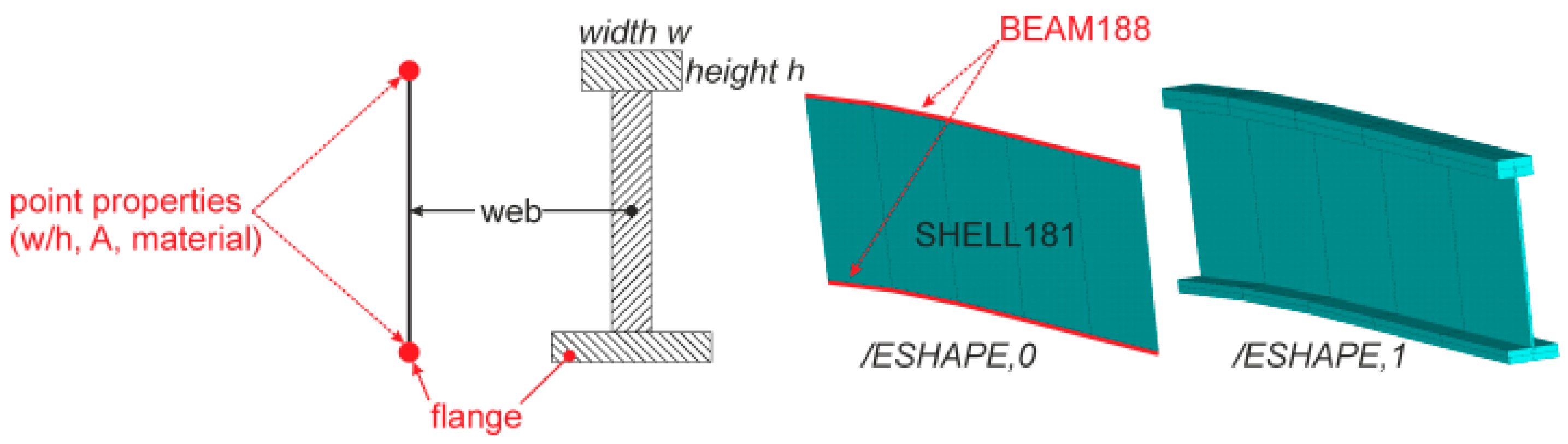
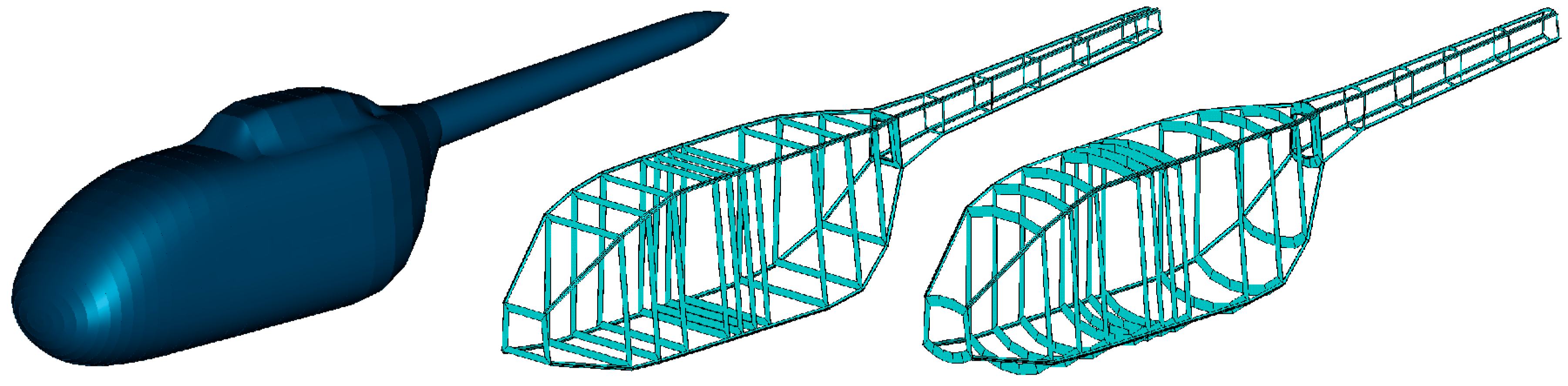
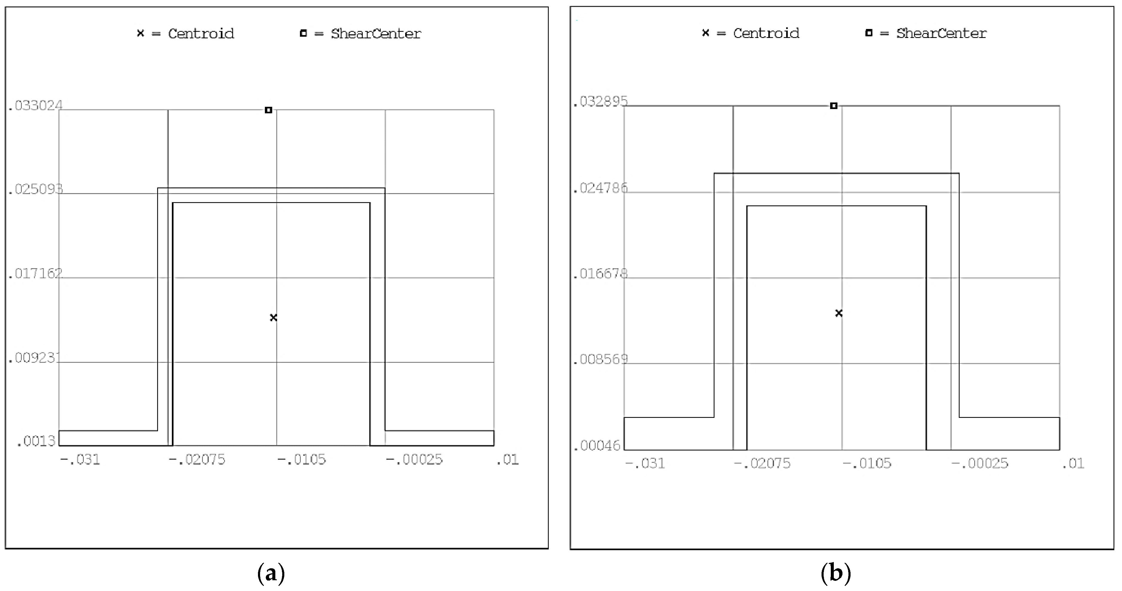
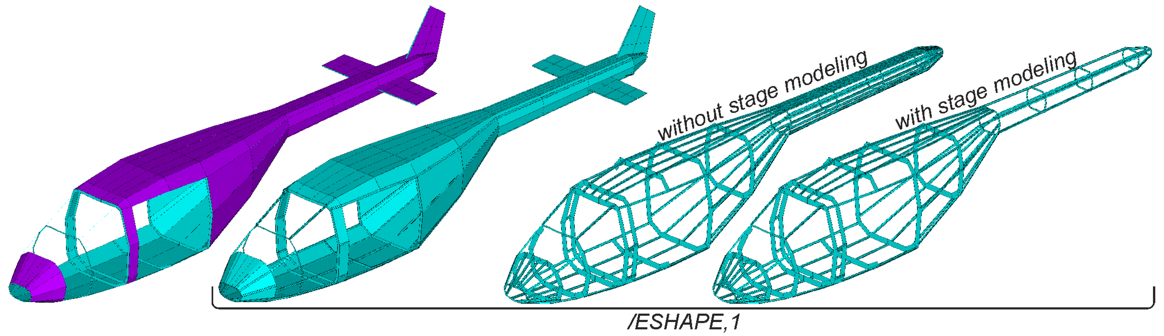
6.2. Model Generation

Taking the outer loft that has been determined during the conceptual design stage as base, a first distribution of the primary structure (frames, stringers, and skin panels) can be conducted. Knowledge based design criteria are used to distribute the skin reinforcements (frames and stringers). For example, cutouts are reinforced to distribute the loads around the cutouts. Additionally, structure must be reinforced where so-called hard points are attached that are used to integrate key components to the fuselage, such as the rotors, gear box, or the alighting gear. Figure 17 schematically presents the process flow for the initial stiffness distribution. During the conceptual design stage, the outer fuselage shape has been elaborated, shown in turquois. Additional information gained in this design stage is stored to the CPACS file, e.g., the flight loads. Other required information, such as the available structural profiles or materials, has to be determined at this stage at the latest and is also stored to the CPACS file. The intended structural distribution is then also saved in the CPACS file for subsequent usage with higher fidelity tools. Exemplary, four different configurations for one fuselage loft are shown in Figure 17, representing four different operational approaches.

Subsequently, the generation of an FE model is conducted. Currently ANSYS is implemented using an APDL (ANSYS Parametric Design Language) approach. The airframe is modeled using an approach introduced by Hunter [31]. Frames are discretized as extruded profiles using elastic shell elements that can be reinforced with additional beam elements along their edges to account for flanges, as shown in Figure 18. Stringers are discretized as beam elements with arbitrary cross sections allowing a direct transfer of the profile data as it is described in CPACS.

By default, the structural mesh is of global quality (GFEM) which means that each bay (being defined by two adjacent stringers and frames) forms one shell element representing a skin panel. An algorithm analyzes the frames and stringers and calculates their intersections. At each intersection an interpolation point is generated serving as node in the following model generation. So-called structural elements (consisting of profiles and material properties) are extruded either in longitudinal (stringers) or circumferential (frames) direction. Considering the stringers this approach would lead to an unreasonable stiffness and weight increase of the tail boom. Therefore, a virtual dummy structural element type none was implemented in the model generation. Dividing a structural member, i.e., stringer or frame, into several stages allows applying different structural elements to one structural member. This approach is called stage modeling and allows the provision with the virtual dummy element. This method is used to virtually reduce the stringers of the tail boom representing a realistic stiffness distribution and weight for the tail. Moreover, stage modeling is used to describe cutouts for passenger or cargo doors. Figure 19 exemplary shows an FE model of a generic utility helicopter airframe with cutouts for the windshield and doors as well as the impact of stage modeling on a tail boom.

The detail level in the preliminary design phase is not well suited for modeling of joint elements, e.g., cleats that connect frames and stringers to each other as well as to the skin panels. In order to take this additional weight into account, an additional weight is added to the fuselage weight, scaled according to the fuselage mass. Shanley [32], for instance, estimates the weight increase due to joints in the range of 20% - 40% of the ideal minimum weight for metallic structures.

As mentioned above, the interpolation points determine the airframe structure. Splines are generated connecting the interpolation points of a structural member. These splines are then used as extrusion path for the beam and shell elements of the stringers and frames. The more interpolation points are available the better a fuselage loft can be created. Virtual dummy elements can be used to artificially increase the amount of interpolation points thus in turn allowing for a more realistic geometrical modeling of an airframe. Figure 20 shows an exemplary airframe with only four stringers defined in the CPACS file. On the left the fuselage outer loft of a generic helicopter is shown. It resembles a Bo105 shape featuring a comparably soft curvature. The structural FE model in the middle shows the approach without any virtual elements leading to a comparably coarse geometry. The model on the right shows the same airframe with additional stringers featuring the virtual dummy elements at the top and bottom side of the fuselage leading to more interpolation points. It can be seen that this model features a smoother bottom and top surface representing the fuselage loft more precisely.

More details on the modeling approach and on specific options, such as the structural element type none, cutouts, and stage modeling are given by Schwinn [33].

The component masses that have been estimated using statistical methods during the conceptual design phase are modeled as lumped masses at additional nodes. They are constrained to the airframe over a user-specified region. External forces and moments generated at the rotors are applied at the nodes describing the rotors. Figure 21 exemplary shows the airframe of a generic fuselage (for visibility reasons the skin panels have been removed) and the two nodal masses representing the main and tail rotor. The red arrows represent the acting forces (lift and anti-torque force) while the magenta lines represent the constraints introducing the load into the structure. Gravity is modeled as an acceleration field acting on all nodes and elements. The loads calculation uses the fuselage weight which has been estimated during the conceptual design phase for the calculation of the required lift forces. A more detailed description of the loads calculation process as it is currently implemented is given by Schwinn et al. [15].

The model is fixed in space at a node close to the computed center of gravity (COG). Potentially remaining forces due to little load inconsistencies during trim are compensated using the inertia relief option. This approach allows the calculation of stresses and strains without dynamic analyses by introducing artificial boundary conditions for equilibrium of forces and moments.

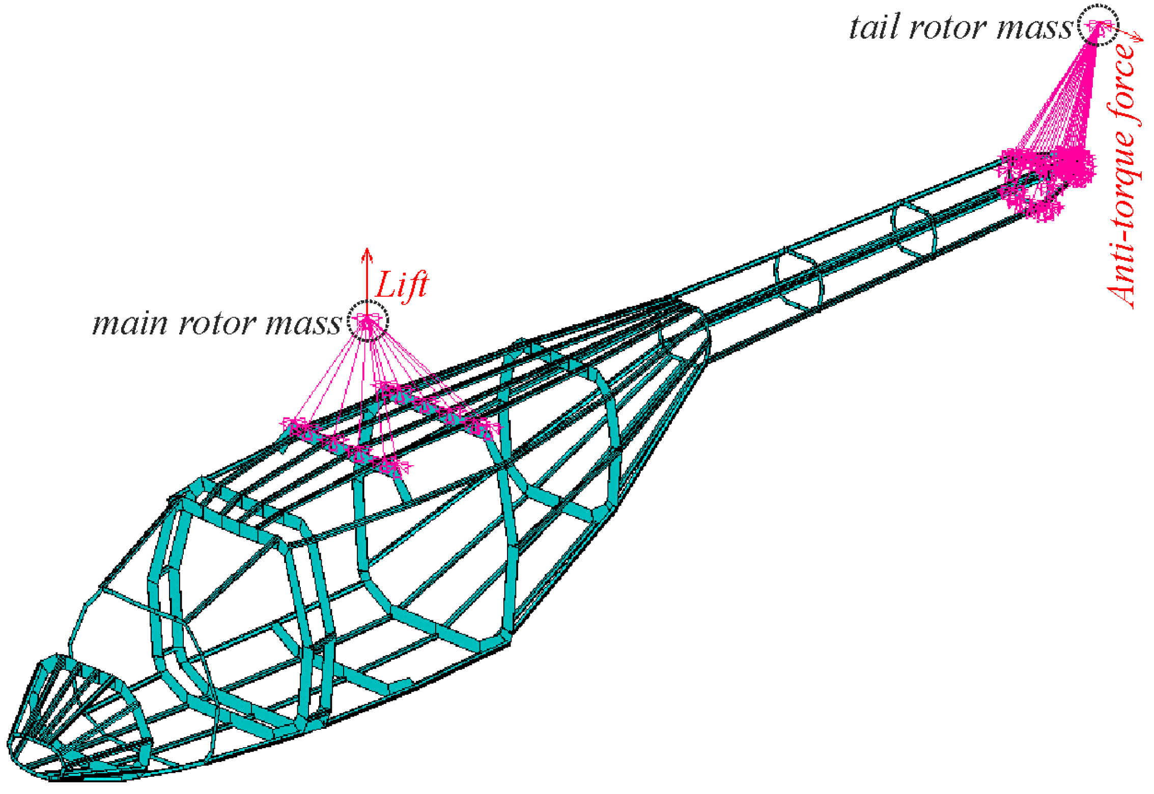
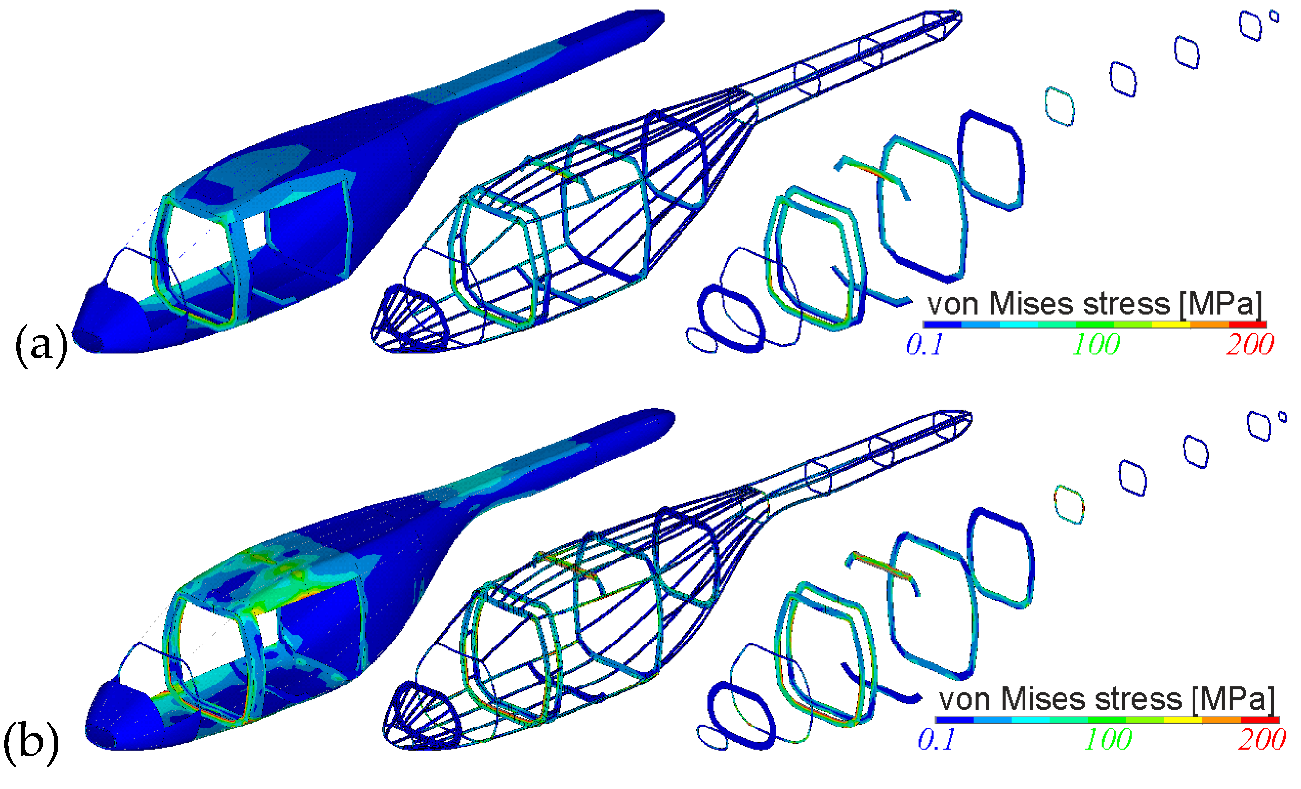
6.3. Static Analysis

Static analyses are conducted using the linear-elastic solver in ANSYS. Exemplary, a hovering analysis of a generic utility rotorcraft with cutouts for two pilot doors, two cabin doors and for the windshield is shown in Figure 22. The complete airframe is made of aluminum 2024 with material properties as given in

Table 10. Aluminum 2024—material properties.

Parameter	Value
Young’s modulus [GPa]	67.7
Density, kg/m3	2800 [kg/m3]
Poisson’s ration, -	0.248
Yield strength, MPa	320

. The stringers feature a hat shaped profile with a constant sheet thickness of $t_{stringer}$ = 1.4 mm. The frames are flat featuring different heights. The thickness of the frames ranges from $t_{stringer}$ = 1.4 mm to $t_{frames,\max }$ = 1.6 mm, while the skin panels all feature a thickness of $t_{skin}$ = 1.0 mm.

The fuselage on the left shows the complete airframe. For visibility reasons the skin panels have been removed in the middle figure allowing a closer look on the frames and stringers. The stringers have been removed in the figure on the right enabling a clearer examination of the frames.

It can be observed from Figure 22a that the highest stresses arise where the heaviest masses are located and the external loads from the rotors are introduced. Especially the center frame where the lift of the main rotor is introduced into the airframe is highly stressed. It can also be seen that due to the fuselage cutouts the load is transferred around the cutout in the adjacent frames while the highest stress is located in the center frame of the cutout where the main rotor is located. Additionally, it can be observed that the lateral (anti-torque) force generated by the tail rotor (to compensate the torque of the main rotor) leads to a stress increase at the transition frame between fuselage cabin and tail boom. The tail boom can be considered as a beam under bending respectively torsional load clamped at the aforementioned transition frame.

Applying a finer discretization in detailed FEM (DFEM) quality to the same model, as shown in Figure 22b, a mesh dependent behavior can be observed. This dependence verifies that the (GFEM) mesh is not fine enough to calculate local stress peaks, so the stresses are averaged over the larger areas, i.e., the larger element sizes. Therefore, localized stress concentrations cannot be adequately shown with the coarse GFEM approach. However, it shall be noted that for preliminary purposes, the GFEM approach is considered as sufficient because of the faster pre- and post-processing, faster computations, and smaller file sizes in relation to the required level of detail.

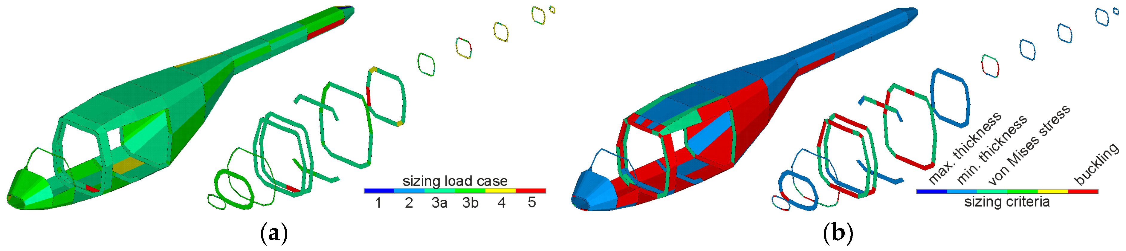
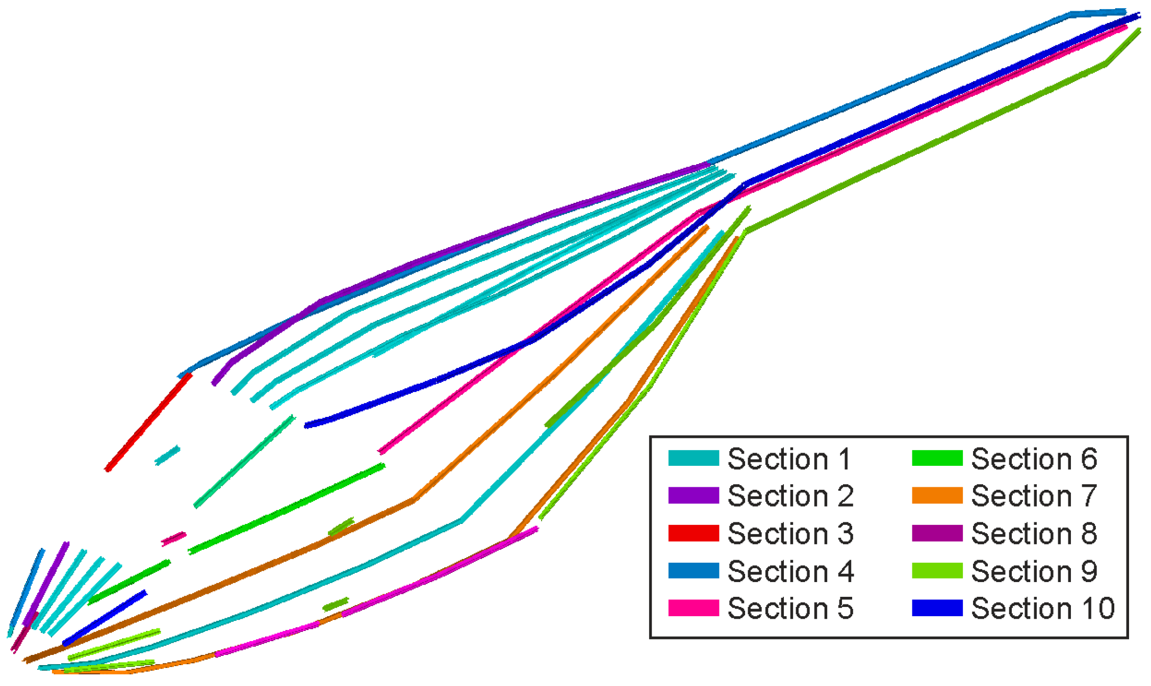
6.4. Sizing Approach

Structural sizing is conducted using an APDL based sizing module that has originally been developed for sizing of aircraft wings (see Nagel [34]), enhanced to size transport aircraft fuselages (see Scherer [35]) and finally extended for the use of rotorcraft (see Schwinn [36]). Strength evaluation is based on fully stressed design (FSD) principles. To guarantee sufficient safety against stability failure, local compressive and shear buckling methods as provided by Bruhn [37] have been implemented. For each element the equivalent stress ${\mathsf{\sigma }}_{eqv}$ is computed. This stress value is then used to individually size the element with a scaling factor $sf$ according to Equation (16).

$$sf=\frac{{\mathsf{\sigma }}_{eqv,\max ,a}}{{\mathsf{\sigma }}_{eqv}}$$

(16)

Here ${\mathsf{\sigma }}_{equ,\max ,a}$ describes the maximum allowable equivalent stress, as specified by the material or stability limits (in the CPACS file). Shell elements are sized by their thickness. Beam elements are sized by a common scale factor for their individual sheet thicknesses. This process is repeated for each specified load case and the maximum required element thickness (respectively sheet thicknesses) are stored. The stress levels in all elements are then recalculated with the updated stiffness distribution until convergence is achieved. The final thicknesses and cross sections are saved in the CPACS file as well as the updated mass breakdown due to the new values for structural mass $m_{struct}$, basic empty mass $m_{BEM}$, and maximum take-off mass $m_{MTOM}$. This step allows feedback to the conceptual design loop to allow a resizing of the external configuration with respect to special performance requirements affecting the structural design. An exemplary sizing process for a light utility helicopter, as illustrated in Figure 21 and Figure 22, is displayed in Figure 23. The load cases that were used for the sizing are listed below in

Table 11. Load case description.

Model Number	Load Case (Added)
01	Hovering
02	01 + maximum cruise velocity
03	02 + jump take-off
04	03 + turns
05	04 + 2.5g pull

.

Figure 23 shows the development of the fuselage mass in logarithmic scale versus the iterations for an increasing number of considered load cases. In general, the sizing process converges after five to six iterations. It can be seen, that the fuselage mass increases with the addition of new load cases. The highest fuselage mass is required when the 2.5 g pull maneuver is taken into account. However, it must be noted that the calculation of this case alone cannot be seen sufficient for the structural sizing since different load cases determine the strength at different locations of the airframe.

The weight estimated using the calibrated AFDD models is represented by the dashed line. The red marker in the converged iteration number six (It-06) with the error bars represents the additional mass denoting the joints (applied to model 05) as proposed by Shanley indicating good agreement of the statistical and the numerical approach at this early design stage. The stringer sizing allowed a wide range, potentially scaling the sheet thicknesses t of each stringer $S_i$ in a range of

$$0.5\cdot t_{Si,original}\le t_{Si,new}\le 5.0\cdot t_{Si,original}$$

(17)

Figure 24 shows the resulting thickness distributions for the shell elements (representing the frames and the skin panels). For visualization reasons the skin panels have been removed on the right figure. It is observable that the skin panels are mostly kept at minimum allowed thickness since the load is taken by the surrounding frames and stringers.

As mentioned above, the airframe is sized due to the influence of different load cases at different areas. Figure 25a shows the shell elements of the airframe and their dependence on the specified load case. The numbers that are specified in the legend refer to the number depicting the individual load case as given in Table 11 and Figure 23 (with load cases 3a and 3b representing different turns). Figure 25b shows the relevant sizing criteria for the shell elements. It can be observed that most of the elements are sized either according to strength limits (maximum von Mises stress), shell bucking criteria, and the minimum thickness criteria. The minimum thickness criterion is applied since the surrounding stringers take a significant share of the load.

Figure 26 visualizes the stringer sizing using different colors displaying the new sheet thicknesses t*. The original model before sizing had an identical stringer distribution, i.e., all stringers had the same material properties and cross section with the thickness $t_0$.

It can be observed in Figure 26 that the original section is kept only at the front below the windshield cutout. The two middle stringers running along the roof of the fuselage were reduced while the stringers marking the edge of the fuselage (running along the tail boom) were increased up to a factor of f = 4.5. The stringers marking the lower edges of the door cutouts feature sizing factors in the range of $2.0\le f\le 2.9$ highlighting the need of cutout reinforcements.

Section 1 (S₁) represents the original stringer profile, as depicted in Figure 27a. Exemplary, section 2 (S₂) is illustrated in Figure 27b. As mentioned above, beam elements are sized by equally scaling their sheet thicknesses. The sheet thicknesses of section 2 correspond to Equation (18).

$$t_{S2}=2.2\cdot t_{S1}$$

(18)

It can be seen that section 2 shows similar but scaled sheet thicknesses compared to the shape of the original omega-hat-shaped geometry S₁.

7. Summary

7.1. Lessons Learnt

The experiences gained during and after the preceding projects lead to the restructuring of the sizing process and development of DLRs rotorcraft design environment IRIS. In the following some major finding and properties are listed, which were directly implemented or led to significant changes in the design environment:

• The design environment needs certain breakpoint between the different computational levels. These give the engineer the opportunity to check consistency of the virtual configuration under investigation.
• Last design studies have proven the general feasibility of integration a flight simulation tool, like HOST in the present case into the design environment. However, a reliable integration of such an extensive tool is a great effort. Numerous extensions have to be implemented, for instance the stepwise approach of the velocity to the trim point, in order to ensure reliable computation in batch-mode and convergence of the trim algorithm.
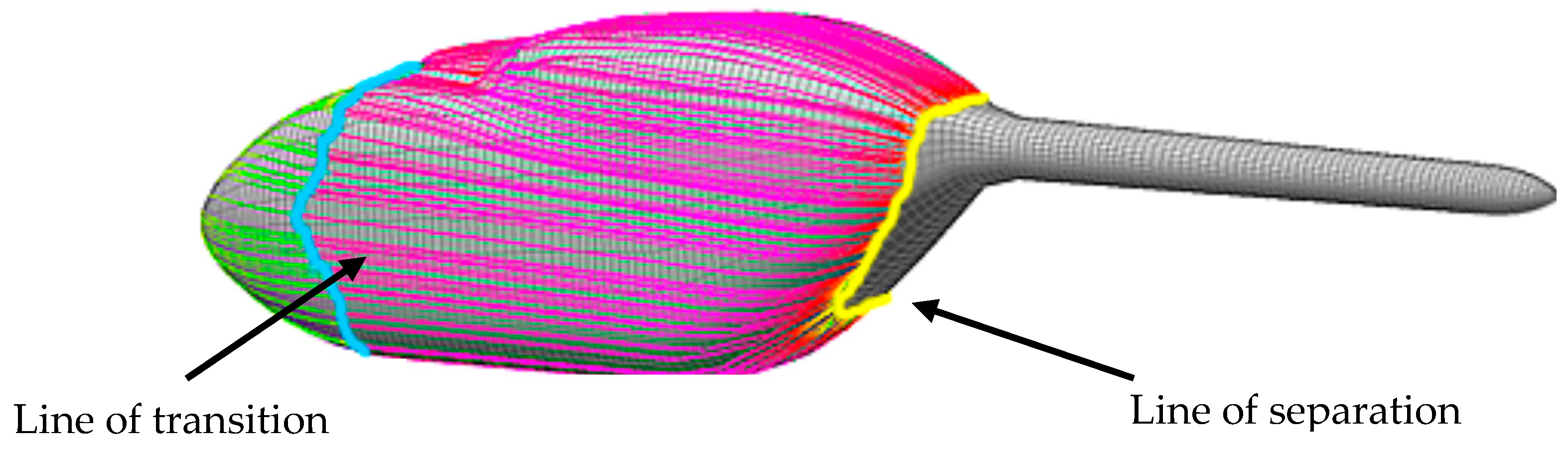
• In the first approach the calculation of the aerodynamic coefficients was conducted inside the level 1 sizing loop. This could also take into account the minor changes of fuselage length. Otherwise the panel method exhibited irregular problems by predicting and handling the area of separated flow on the rear part of fuselage. The computation of the longitudinal force showed a good agreement with reference data from different flight simulation models, but the moment coefficient around all three axes showed errors compromising the trim and performance calculation.
• At the beginning the tool levels were classified by the characteristics of accuracy or uncertainties and computation time. The amount of required input showed to be proportional to the computation time and was added in the next step. Finally, the robustness was added proportional to the uncertainties. The evaluation of the latter showed to be not less important, sometimes even more important than the other three characteristics.
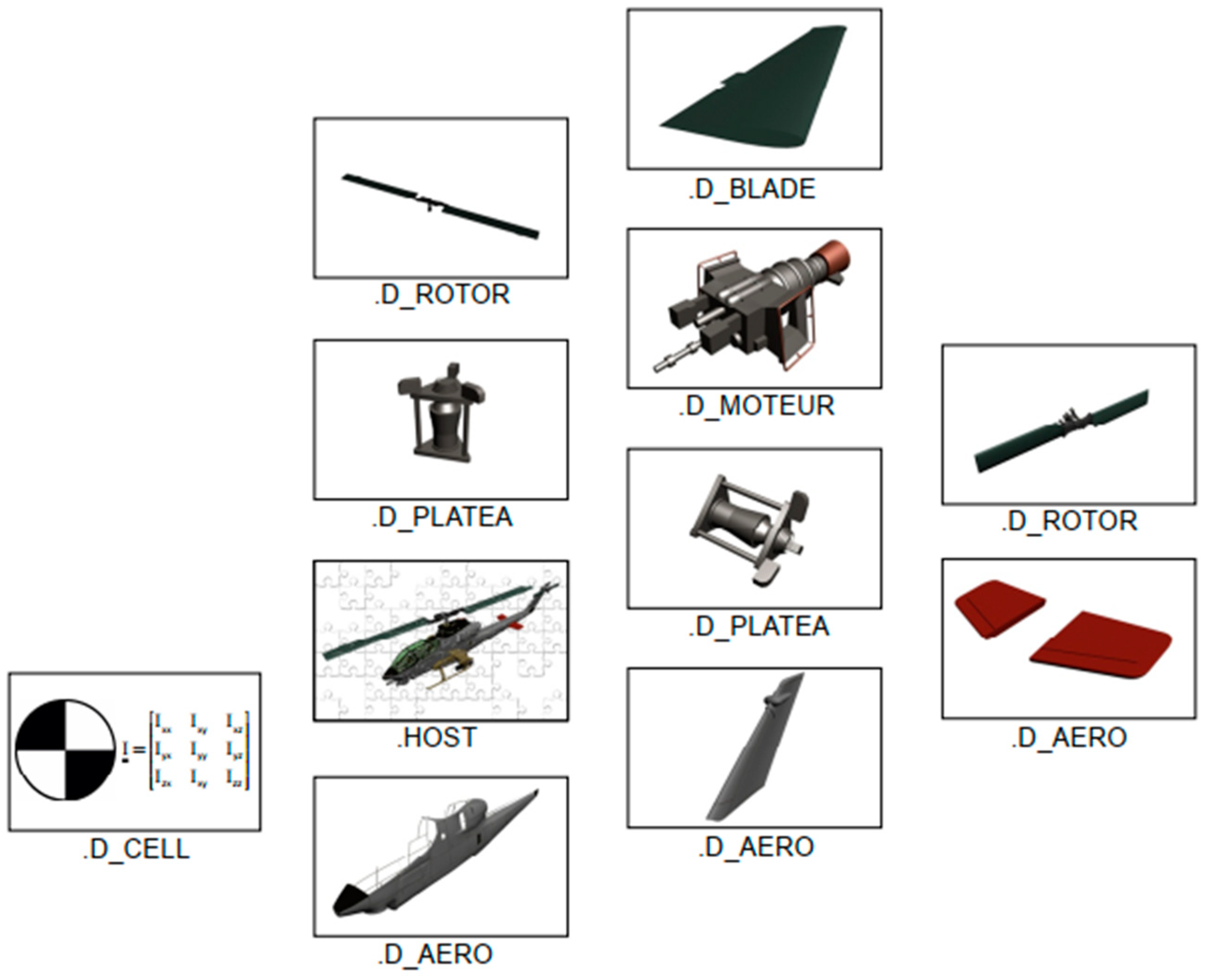
• Applying a uniform data model for every tool leads, sooner or later, to the problem of redundant data, which is an inherent source of errors. The tool specific data in the CPACS model allows the storage of temporary data for every tool. There is still intermediate data which is subsequently processed by other tools. Due to the fact that this data is valid but not final it has to be stored at a different process specific location for temporary data. One example for such data are the dimensions of the fuselage components that are required for the generation of the 3D geometry model.

7.2. Conclusions and Outlook

The features shown in this paper mark the core of the new design environment IRIS. It was essentially possible to follow the guidelines of fixed-wing design in order to show a substantial overlap in the DLR doctrine for aircraft and rotorcraft design. The following capabilities showed to be highly beneficial:

• A high grade of modularity allowing an easy integration, rearrangement and coupling of tools. Now it is an easy task to build different workflows for rotorcraft design including tools developed by different partners and located on different servers.
• The sizing task and especially the flight performance computation is conducted with a sophisticated level of fidelity due to the integration of the higher fidelity overall simulation tool HOST into the workflow. Now the sizing task and the comprehensive analysis are using the same codes for computation. This results in a considerable reduction of uncertainties.
• The integration of the uniform data model CPACS in connection with the collaboration software RCE into the design environment allows an unlimited change between different levels of design. This virtually merges the phase of conceptual design with a wide range of the preliminary design phase. The ability to couple the conceptual design with a variety of comprehensive analysis tools for optimization is now available and outperforms the previous approaches.
• The second benefit in the harmonization with the CPACS data model is the easy coupling of the workflows with workflows of other institutes also using CPACS, which, however, are not integrated into the rotorcraft design project. This DLR doctrine allows the bringing together of independently working projects.

The prospective research objectives for next generation rotorcraft configurations include distributed thrust and lift, new control laws and new propulsion concepts and show the need for more sophisticated and highly modular sizing approach. Besides of the flight physics today there are other assessment and optimization goals in terms of product life cycle management for instance life-cycle costs and environmental impact. The DLR institute for Maintenance, Repair and Overhaul in Hamburg already expressed the demand for modular design environment operation with the CPACS data model to couple design chains with life cycle assessment. Therefore, since the conceptual design is the basis for every short or extensive design study, the further development will build on the present toolbox and extend it.

References

- Raymer, D.P. Aircraft Design. A Conceptual Approach, 5th ed.; AIAA Education Series; AIAA American Institute of Aeronautics and Astronautics: Reston, VA, USA, 2012. [Google Scholar]
- Johnson, W. NDARC—NASA Design and Analysis of Rotorcraft; NASA/TP–2009-215402; Ames Research Center: Moffett Field, CA, USA, 2009.
- Sinsay, J.D. Re-imagining Rotorcraft Advanced Design. In Proceedings of the Rotorcraft Virtual Engineering Conference, Liverpool, UK, 8–10 November 2016. [Google Scholar]
- Johnson, W.; Moodie, A.M.; Yeo, H. Design and Performance of Lift-Offset Rotorcraft for Short-Haul Missions; American Helicopter Society Future: San Francisco, CA, USA, 2012. [Google Scholar]
- Lawrence, B. Handling Qualities Optimization for Rotorcraft Conceptual Design. In Proceedings of the Rotorcraft Virtual Engineering Conference, Liverpool, UK, 8–10 November 2016. [Google Scholar]
- Basset, P.-M.; Tremolet, A.; Cuzieux, F.; Reboul, G.; Costes, M.; Tristrant, D.; Petot, D. CREATION the Onera Multi-Level Rotorcraft Concepts Evaluation Tool: The Foundations. In Proceedings of the Future Vertical Lift Aircraft Design Conference, San Francisco, CA, USA, 18–20 January 2012. [Google Scholar]
- Russell, C.; Basset, P.-M. Conceptual Design of Environmentally Friendly Rotorcraft—A Comparison of NASA and ONERA Approaches. In Proceedings of the AHS 71st Annual Forum, Virginia Beach, VA, USA, 5–7 May 2015. [Google Scholar]
- Boer, J.-F.; Stevens, J. Helicopter Life Cycle Cost reduction through pre-design optimisation. In Proceedings of the 32nd European Rotorcraft Forum, Maastricht, NL, USA, 12 September 2006. [Google Scholar]
- Weiand, P.; Krenik, A. A multi-disciplinary toolbox for rotorcraft design. Aeronaut. J. 2018, 122, 620–645. [Google Scholar] [CrossRef]
- Nicolai, L.M.; Carichner, G.E. Fundamentals of Aircraft and Airship Design; AIAA Education Series; AIAA American Institute of Aeronautics and Astronautics: Reston, VA, USA, 2010. [Google Scholar]
- Roskam, J. Airplane Cost estimation. Design, Development, Manufacturing and Operating, 3rd ed.; Roskam Aviation and Engineering Corporation: Lawrence, KS, USA, 2006. [Google Scholar]
- Layton, D.M. Introduction to Helicopter Design; AIAA Professional Studies Series; AIAA: Salinas, CA, USA, 1992. [Google Scholar]
- Liersch, C.M.; Hepperle, M. A distributed toolbox for multidisciplinary preliminary aircraft design. CEAS Aeronaut. J. 2011, 2, 57–68. [Google Scholar] [CrossRef]
- Liersch, C.M.; Huber, K.C. Conceptual Design and Aerodynamic Analyses of a Generic UCAV Configuration. In Proceedings of the 32nd AIAA Applied Aerodynamics Conference, Atlanta, GA, USA, 16 June 2014. [Google Scholar]
- Schwinn, D.; Weiand, P.; Schmid, M.; Buchwald, M. Structural sizing of a rotorcraft fuselage using an integrated design approach. In Proceedings of the 31th Congress of the International Council of the Aeronautical Sciences, Belo Horizonte, Brazil, 9–14 September 2018. [Google Scholar]
- Bachmann, A.; Kunde, M.; Litz, M.; Schreiber, A. Advances in Generalization and Decoupling of Software Parts in a Scientific Simulation Workflow System. In Proceedings of the 4th International Conference on Advanced Engineering Computing and Applications in Sciences—ADVCOMP 2010, Florence, Italy, 25–30 October 2010. [Google Scholar]
- Seider, D.; Fischer, P.M.; Litz, M.; Schreiber, A.; Gerndt, A. Open Source Software Framework for Applications in Aeronautics and Space. In Proceedings of the IEEE Aerospace Conference, Big Sky, MT, USA, 3 March 2012. [Google Scholar]
- Böhnke, D.; Litz, M.; Rudolph, S. Evaluation of Modeling Languages for Preliminary Airplane Design in Multidisciplinary Design Environments. In Proceedings of the 2010 Deutscher Luft-und Raumfahrtkongress, Hamburg, Germany, 31 August–3 September 2010. [Google Scholar]
- Nagel, B.; Böhnke, D.; Gollnick, V.; Schmollgruber, P.; Rizzi, A.; La Rocca, G.; Alonso, J.J. Communication in Aircraft Design: Can we establish a common language? In Proceedings of the 28th International Congress of the Aeronautical Science, Brisbane, Australia, 23–28 September 2012. [Google Scholar]
- Benoit, B.; Dequin, A.-M.; Kampa, K.; Grünhagen, W.; von Basset, P.-M.; Gimonet, B. HOST, a General Helicopter Simulation Tool for Germany and France. In Proceedings of the American Helicopter Society 56th Annual Forum, Virginia Beach, VA, USA, 2–4 May 2000. [Google Scholar]
- Van der Wall, B.G. Grundlagen der Hubschrauber-Aerodynamik, 1st ed.; VDI-Buch; Springer: Berlin/Heidelberg, Germany, 2015. [Google Scholar]
- Kunze, P. Parametric Fuselage Geometry Generation and Aerodynamic Performance Prediction in Preliminary Rotorcraft Design. In Proceedings of the 39th European Rotorcraft Forum, Moscow, Russia, 3–6 September 2013. [Google Scholar]
- Maskew, B. Program VSAERO Theory Document—NASA CR-4023; NASA: Redmond, WA, USA, 1987.
- Keys, C.N.; Wiesner, R. Guidelines for Reducing Helicopter Parasite Drag. J. Am. Helicopter Soc. 1975, 20, 31–40. [Google Scholar] [CrossRef]
- Stepniewski, W.Z. Rotary-Wing Aerodynamics. In Dover Books on Aeronautical Engineering; Dover Publications: Newburyport, MA, USA, 2013. [Google Scholar]
- Krenik, A.; Weiand, P. Aspects on Conceptual and Preliminary Helicopter Design. In Proceedings of the 2016 Deutscher Luft-und Raumfahrtkongress, Braunschweig, Germany, 13–15 September 2016. [Google Scholar]
- Beltramo, M.N.; Morris, M.A. Parametric Study of Helicopter Aircraft Systems Costs and Weights—NASA-CR-152315; NASA: Moffett Field, CA, USA, 1980.
- Palasis, D. Erstellung eines Vorentwurfsverfahrens für Hubschrauber Mit Einer Erweiterung für das Kipprotorflugzeug; VDI-Verlag: Düsseldorf, Germany, 1992; Volume 201. [Google Scholar]
- Prouty, R.W. Helicopter Performance, Stability, and Control; Krieger: Malabar, FL, USA, 2005. [Google Scholar]
- Kaletka, J.; Kurscheid, H.; Butter, U. FHS, the new research helicopter: Ready for service. Aerosp. Sci. Technol. 2005, 9, 456–467. [Google Scholar] [CrossRef]
- Hunter, E. A Process Enabling High Fidelity Airframe Sizing and Optimization for Conceptual Design. In Proceedings of the 49th AIAA/ASME/ASCE/AHS/ASC Structures, Structural Dynamics, and Materials Conference, Schaumburg, IL, USA, 7 April 2008. [Google Scholar]
- Shanley, F.R. Weight-Strength Analysis of Aircraft Structures, 2nd ed.; Dover Publ: New York, NY, USA, 1960. [Google Scholar]
- Schwinn, D.B. Applied parametrized and automated airframe modeling methods in the preliminary design phase. Int. J. Model. Simul. Sci. Comput. 2015, 6, 1550037. [Google Scholar] [CrossRef]
- Nagel, B.; Kintscher, M.; Streit, T. Active and Passive Structural Measure for Aedrolastic Winglet. In Proceedings of the 26th International Congress of the Aeronautical Sciences, Anchorage, AK, USA, 14–19 September 2008. [Google Scholar]
- Scherer, J.; Kohlgrüber, D.; Dorbath, F.; Sorour, M. A Finite Element Based Tool Chain for Structural Sizing of Transport Aircraft in Preliminary Aircraft Design. In Proceedings of the 2013 Deutscher Luft-und Raumfahrtkongress, Stuttgart, Germany, 10–12 September 2013. [Google Scholar]
- Schwinn, D.; Weiand, P.; Schmid, M. Structural Analysis of a Rotorcraft Fuselage in a Multidisciplinary Environment. In Proceedings of the NAFEMS World Congress, Stockholm, Sweden, 11–14 June 2017. [Google Scholar]
- Bruhn, E.F. Analysis and Design of Flight Vehicle Structures; Jacobs Publishing: Indianapolis, IN, USA, 1973. [Google Scholar]