Model-Based Fault Detection and Diagnosis for Spacecraft with an Application for the SONATE Triple Cube Nano-Satellite


Abstract
1. Introduction
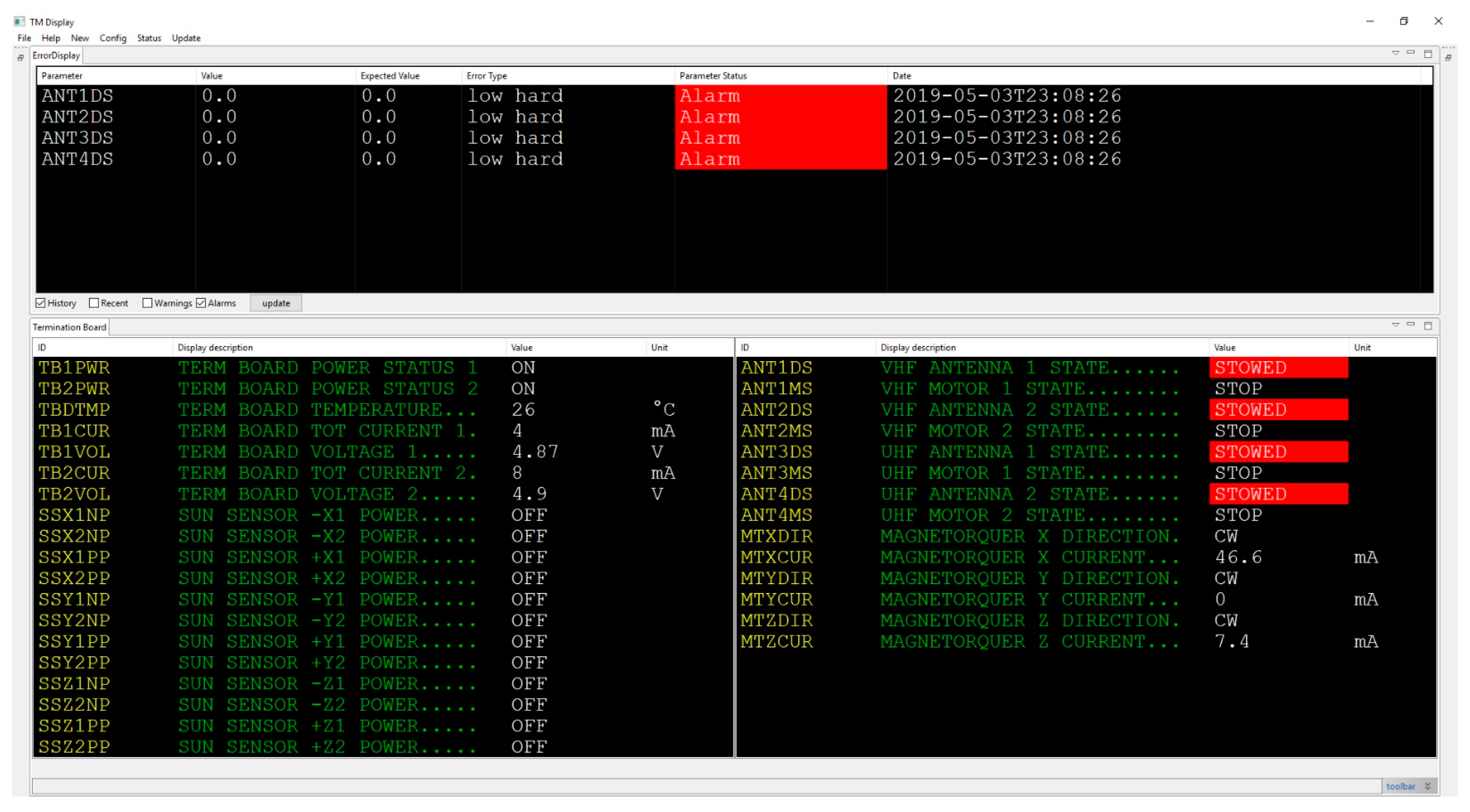
2. Classical Health Monitoring and Fault Detection
3. Model-Based Diagnosis
3.1. Model and Simulator
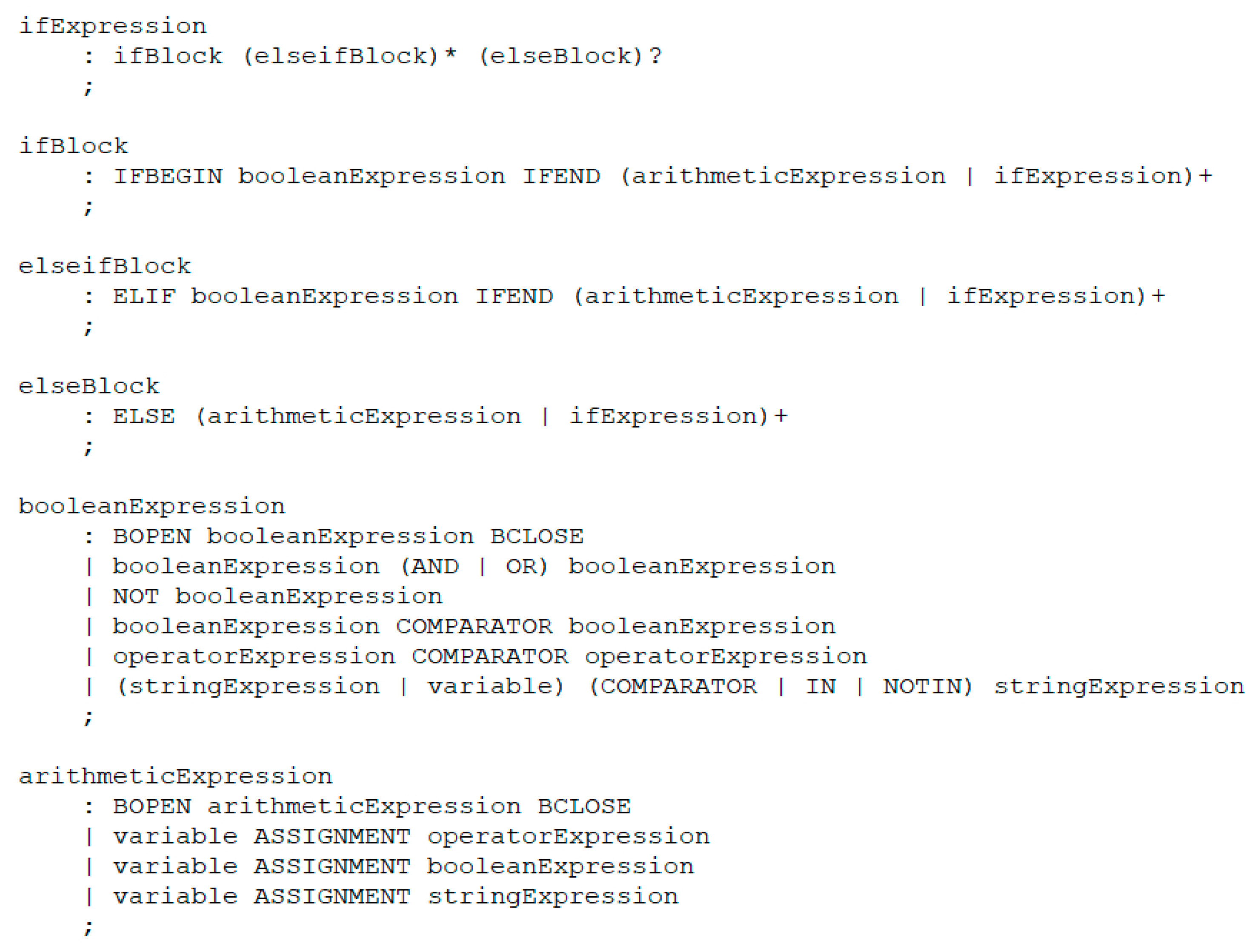
3.1.1. Model Editor
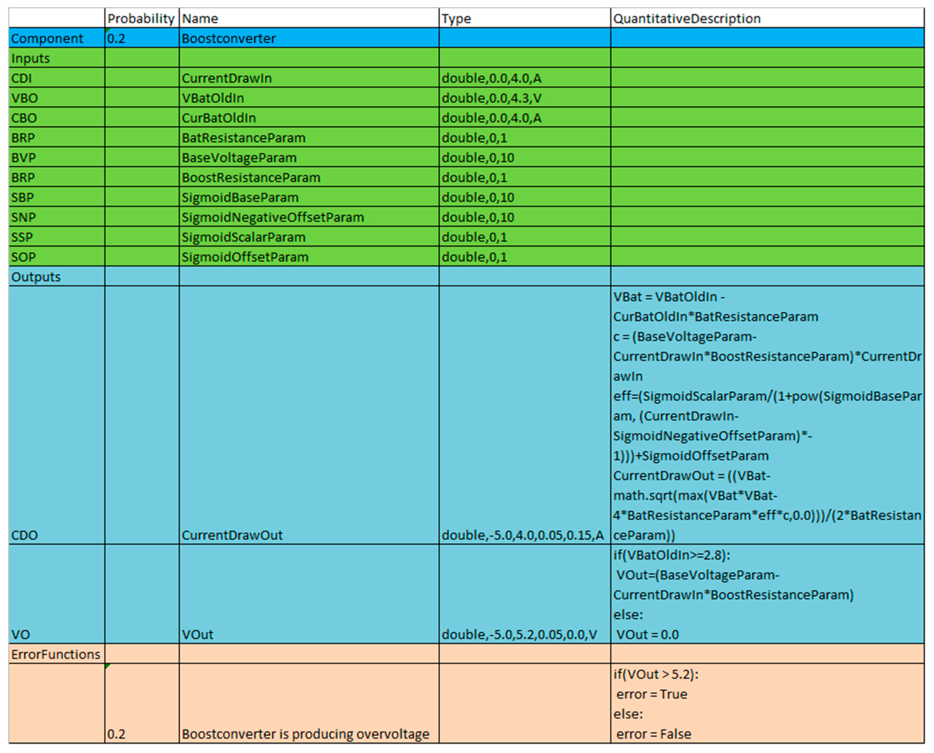
3.1.2. Component Class Format
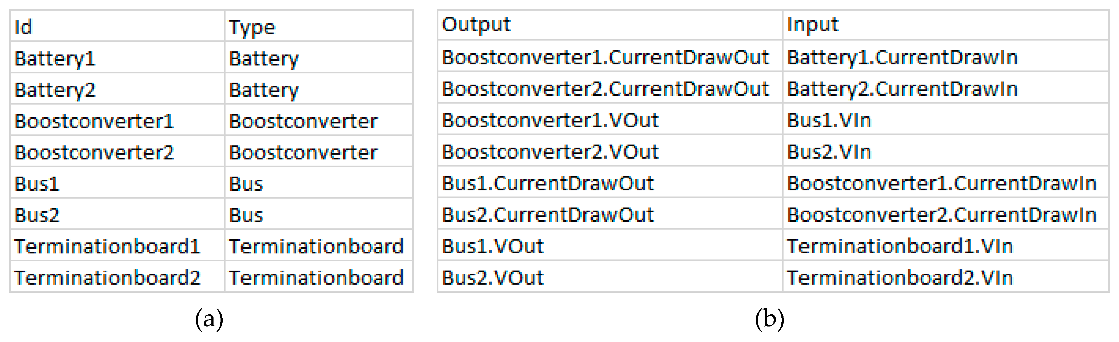
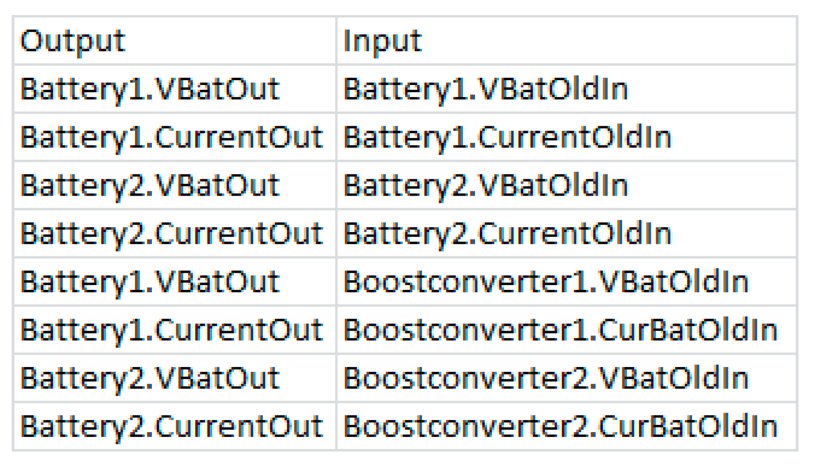
3.1.3. Connector Format
3.1.4. Port Dependencies
- The static port dependencies map each outport of each component to the inports that are needed to compute a value for the corresponding outport, independent of the actual inport values. These port dependencies are all inports, which are part of the quantitative description of the corresponding outport. When the outport of a component is simulated, it is first checked, if the values for all inports on which the outport is dependent are available.
- The dynamic port dependencies are used for the computation of conflict sets during the diagnosis. These port dependencies map each outport of each component to the inports on which the corresponding outport is dependent during the current time step, given the available values for the inports. These port dependencies are updated after each simulation, since the port dependencies can change in respect to the values of the inports.
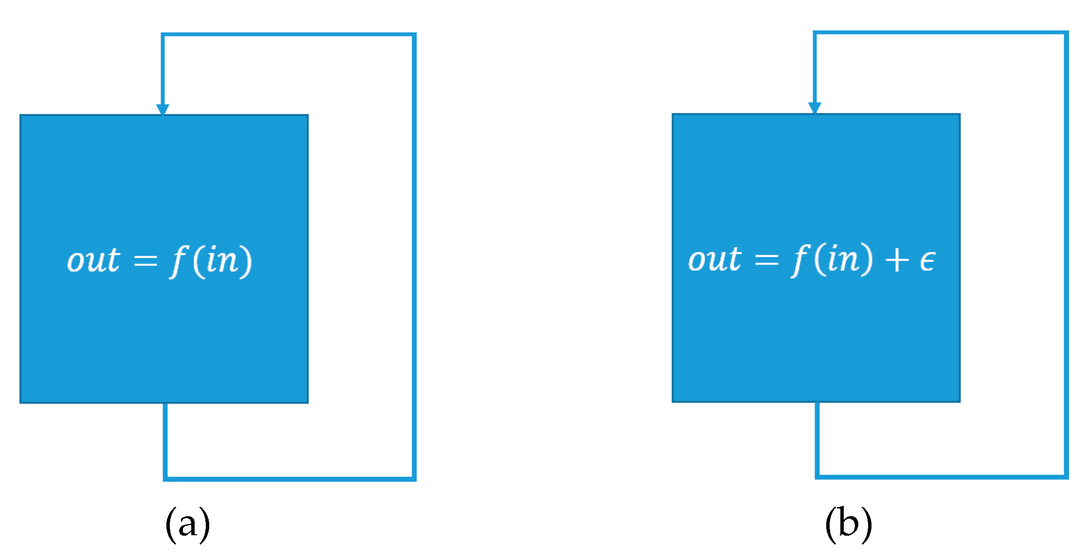
3.2. Simulation
| Algorithm 1. Pseudo code of the SimulateInitial-function of the simulator, used to perform initial computations e.g., the simulation of emitters and to initialize the necessary data structures for further simulation of the model. |
| ALGORITHM: SimulateInitial INPUTS: The set of simulated outputs from the previous iteration: The set of measured inputs from the current iteration: The set of measured outputs from the current iteration: The set of model components: The set of forward connections: The set of backward connections: OUTPUTS: The set of simulated outputs: 1. Map outputs from to inputs , using 2. Let be an empty set of input values. Merge and into 3. Map all outputs from to inputs, using and merge them with 4. Let be an empty set of output values 5. Let be an empty set of components to consider for simulation 6. Let be an empty map of components to sets of ports to keep track which ports of which components have been simulated already 7. Determine the set of components , that cannot be simulated during the current iteration of the simulation 8. Simulate all emitter components, map their outputs to inputs and merge them with . Add all components connected to them that are not in to 9. Check and add all components, that have at least one and are not in to 10. IF THEN SimulateRecursive(, , , , , ) ELSE RETURN |
| Algorithm 2. Pseudo code of the SimulateRecursive-function of the simulator, used to perform the simulation of model components in a recursive fashion. |
| ALGORITHM: SimulateRecursive INPUTS: The set of all input values: The set of forward connections: The set of unsimulatable components: The set of current candidates: The map of currently simulated components: The set of currently simulated outputs: OUTPUTS: The set of simulated outputs: 1. Let be an empty set of components to consider for simulation 2. FOR EACH IF has ports that are simulatable and are not contained in THEN simulate new simulatable ports Merge into Map to inputs, using and merge them with IF contains all outports of THEN is finished and won’t be considered again for simulation Add all components connected to to 3. IF THEN SimulateRecursive(, , , , , ) ELSE RETURN |
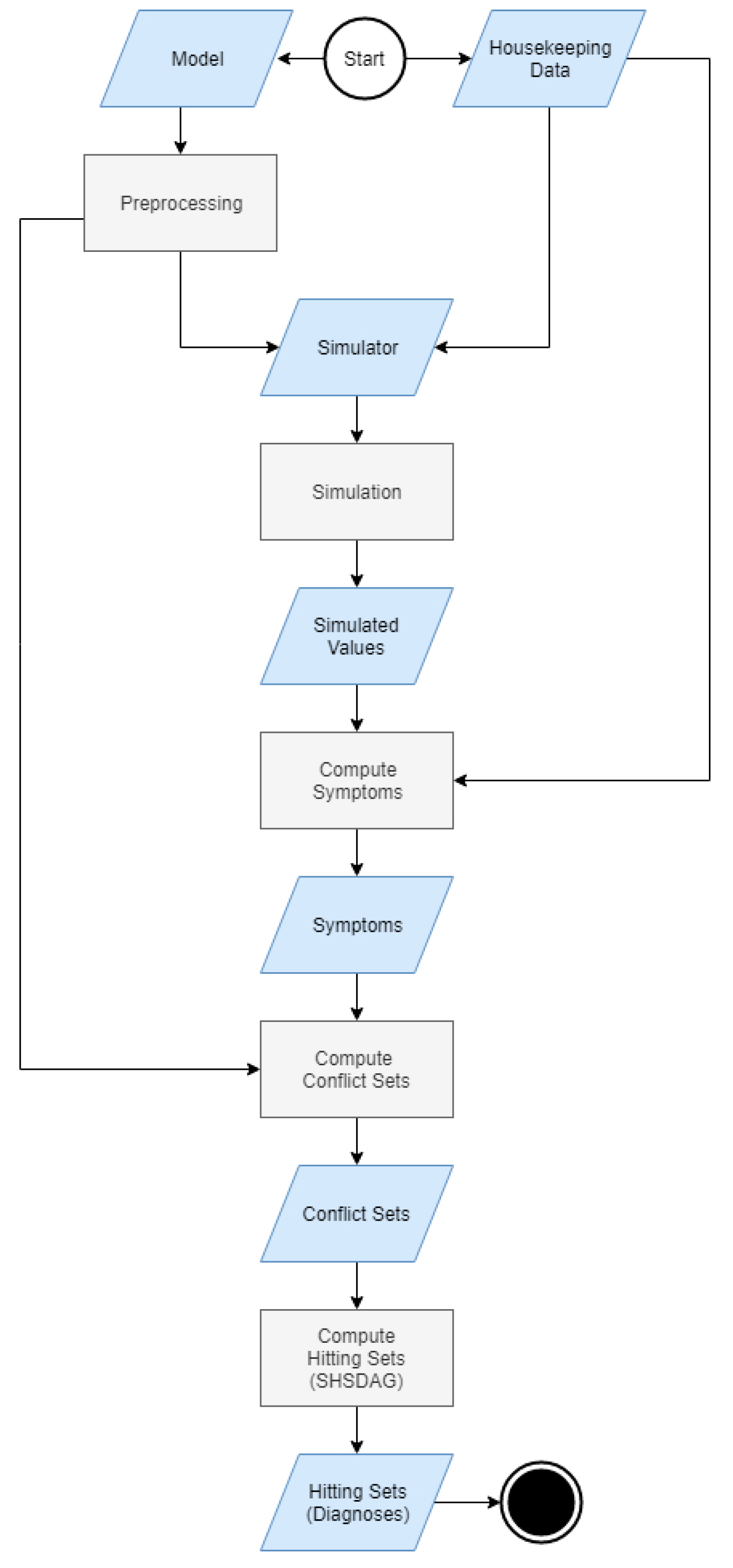
3.3. Diagnostic Algorithm
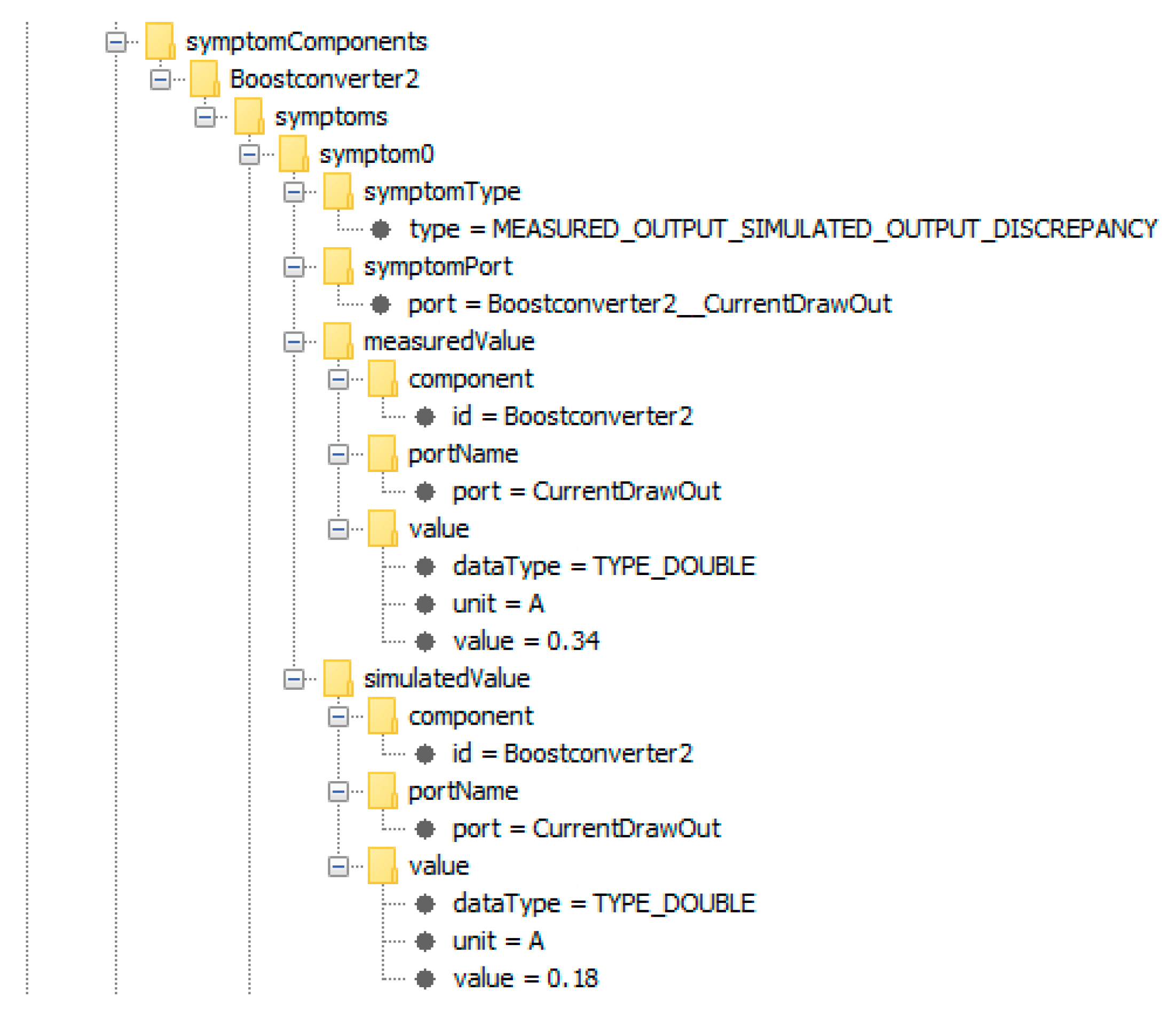
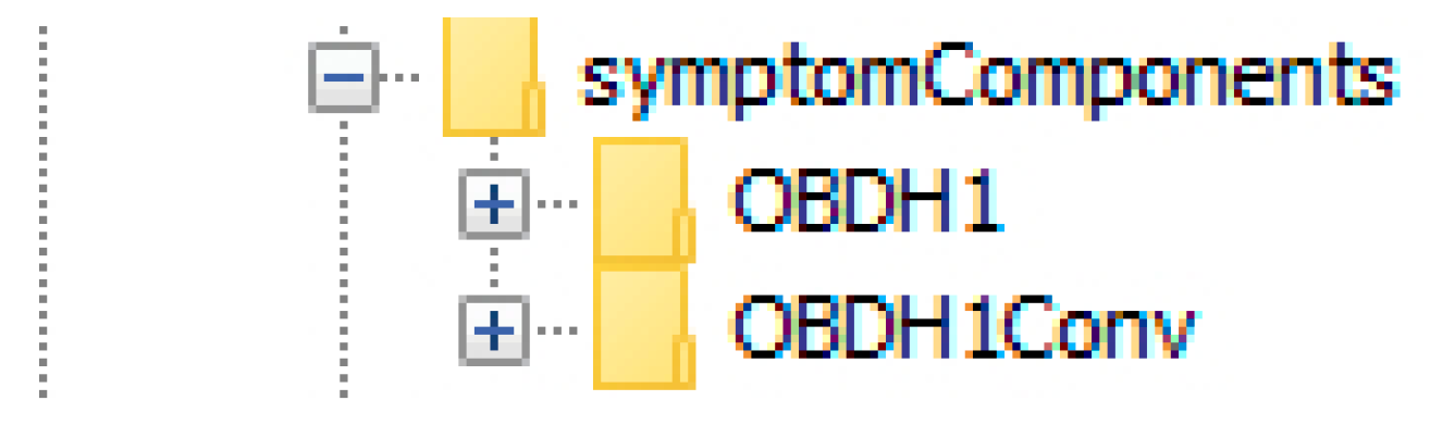
3.3.1. Symptoms
- The measured value of an outport is smaller than its lower threshold limit
- The measured value of an outport is greater than its upper threshold limit
- The deviation of the measured value of an outport from its corresponding simulated value violates its tolerance intervals
3.3.2. Computation of Conflict Sets
| Algorithm 3. Pseudo code of the ComputeConflictSet-function used to compute a conflict set, given a symptom component, so that a malfunction of a component of the conflict set would explain the observed symptoms of the symptom component. |
| ALGORITHM: ComputeConflictSet INPUTS: The symptom component to compute a conflict set for: The dynamic port dependencies: The set of measured outputs of the current iteration: The model graph: The set of all symptom components: The set of all excluded components: The model state of the previous iteration: OUTPUTS: The conflict set corresponding to and the map of components to sets of suspecting components 1. Let be an empty set of output ports. Merge the symptom ports of the symptoms associated with into 2. Let be an empty map of components to sets of suspecting components 3. Use to compute for each the inputs on which is dependent and use to identify the output ports , which are connected to the input ports of . Search the whole model graph using a backwards directed breadth-first search. Replace with before continuing with the next level. Before visiting a component through an output port , take an action based on the following conditions:
4. RETURN and |
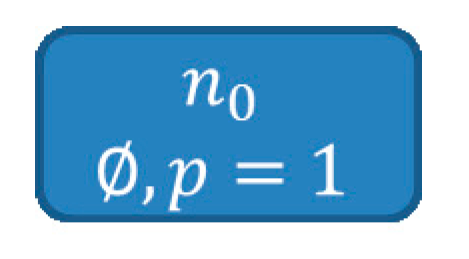
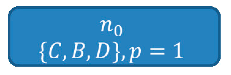
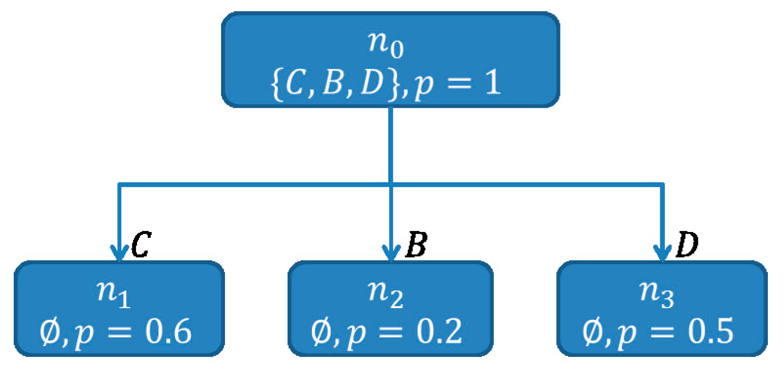
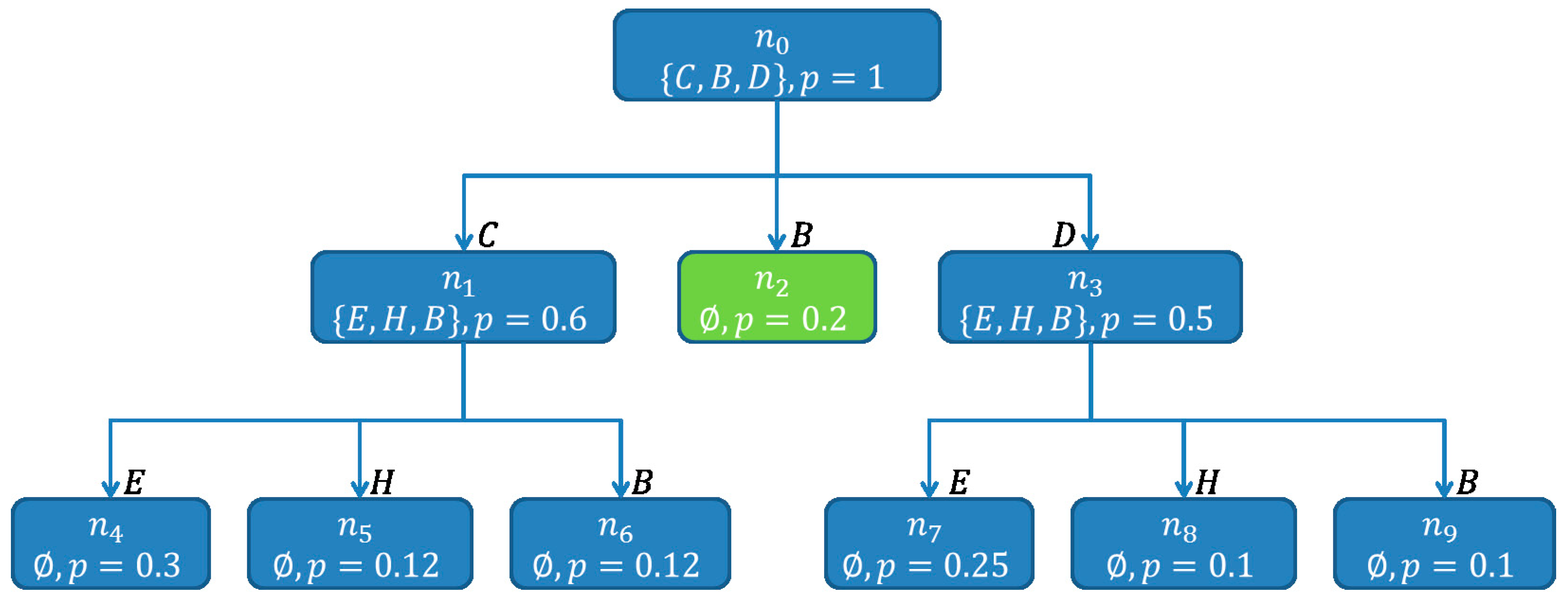
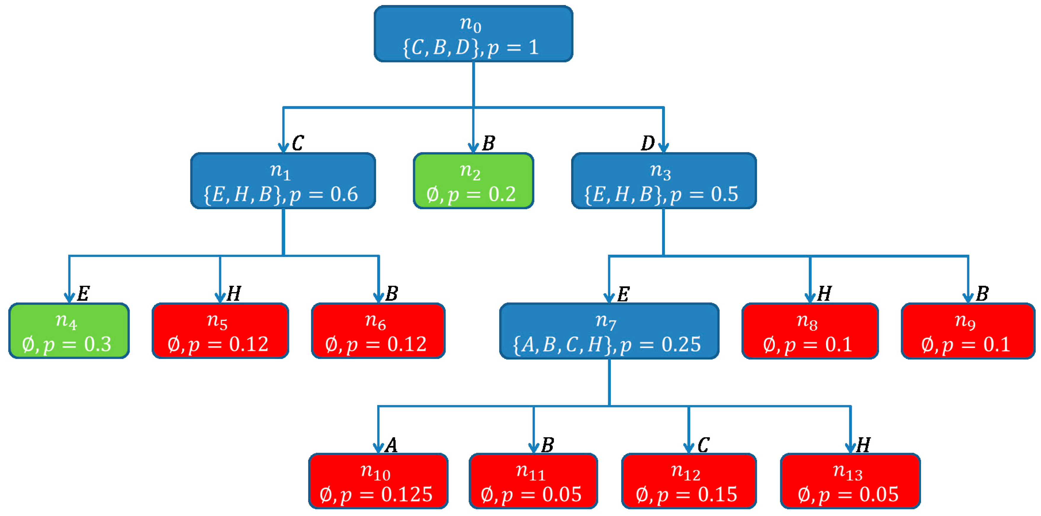
3.3.3. Computation of Hitting Sets
| Algorithm 4. Pseudo code of the BuildSHSDAG-function used to build a Scored Hitting Set Directed Acyclic Graph (SHSDAG) and therefore to compute the minimal hitting sets, given a set of conflict sets. |
| ALGORITHM: BuildSHSDAG INPUTS: The set of all conflict sets: OUTPUTS: The SHSDAG: SHSDAG 1. Use logical absorption on the 2. Sort ascending by cardinality 3. Let be the empty root node of the SHSDAG 4. Let be an empty list of nodes 5. Let be an empty list of nodes 6. Add to 7. WHILE is not empty FOR EACH Let be the set of edge labels of the path from to FOR EACH IF THEN Label with BREAK IF was labeled with THEN FOR EACH Let be an empty node with state Add as child node to Set the path of to Label the edge from to with Compute a score for based on its new path Add to ELSE Set the state of to Set to Set to an empty list of nodes 8. RETURN the SHSDAG |
- , when has child nodes
- , when the path from to is a dead end and does not correspond to a hitting set
- , when the path from to corresponds to a minimal hitting set
- If a new child node for a node is to be created, due to a component , while there exists a node , with , then is not created, but is added to the child nodes of .
- If the SHSDAG contains a node after a node has been created, with , then close
- If the score cut-off is used with a cut-off factor and the score of a newly created node is , then close node
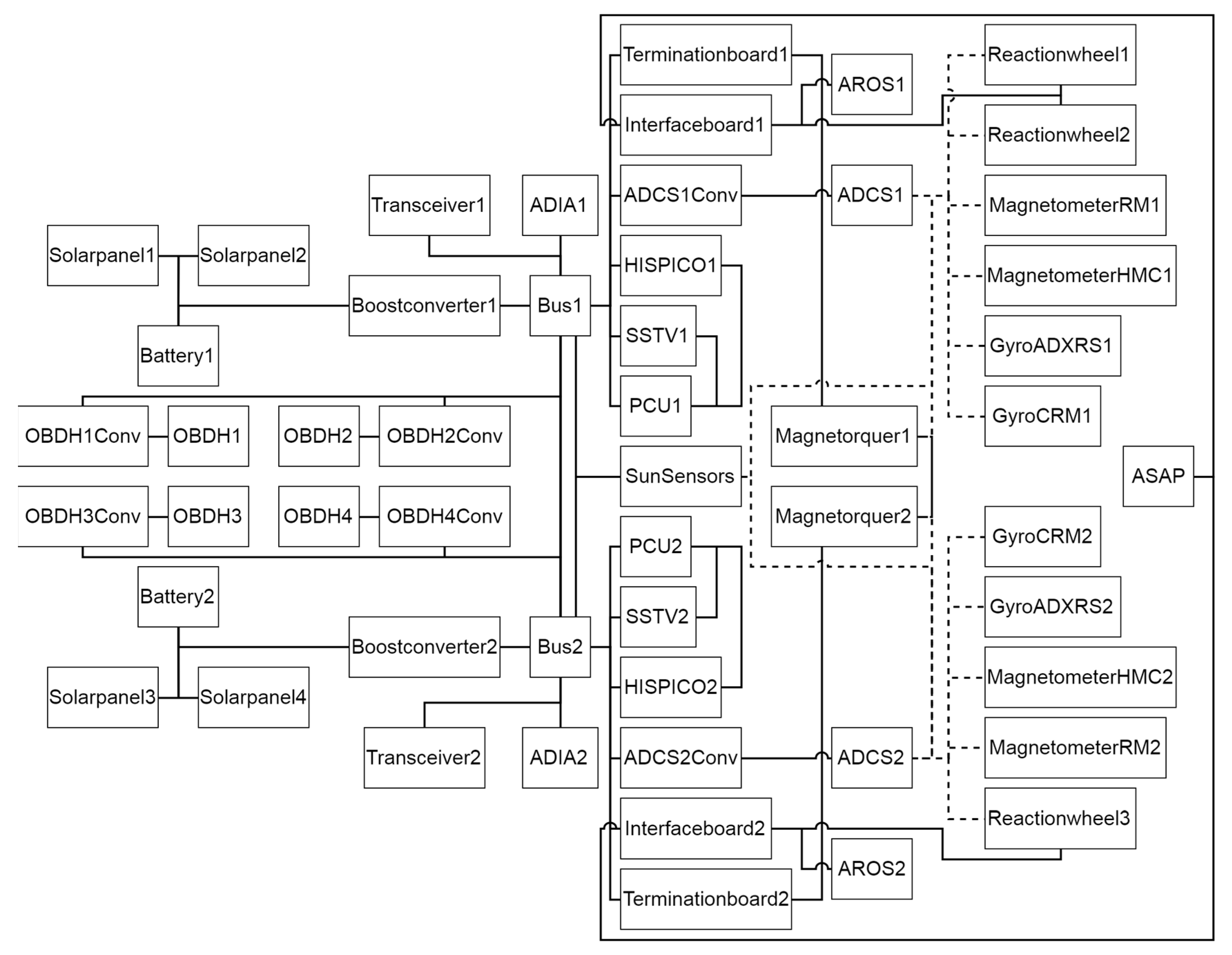
4. Satellite Model
4.1. Model Calibration
4.2. Data and Interfaces
5. Experiments
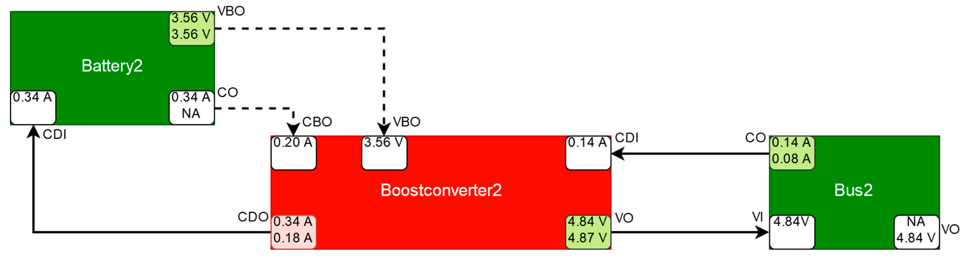
5.1. Boost Converter Malfunction
5.2. Transceiver Malfunction
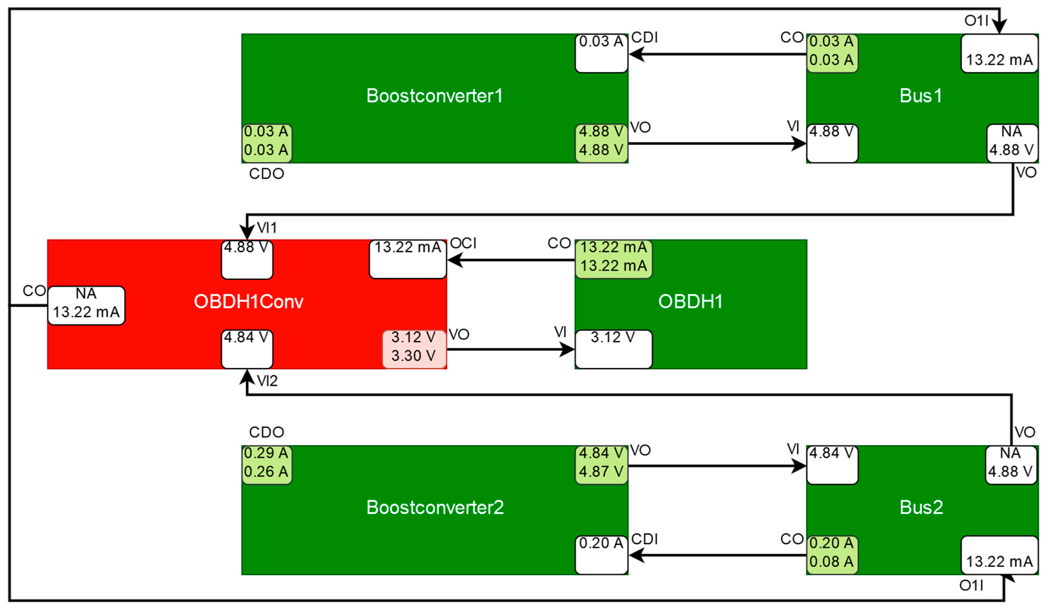
5.3. OBDH Voltage Converter Malfunction
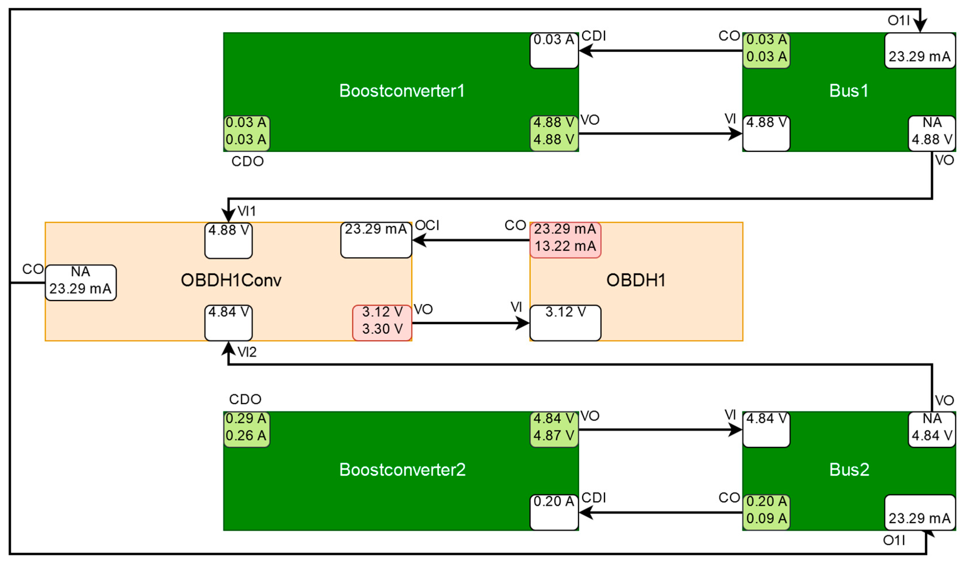
5.4. OBDH Voltage Converter and OBDH Malfunction
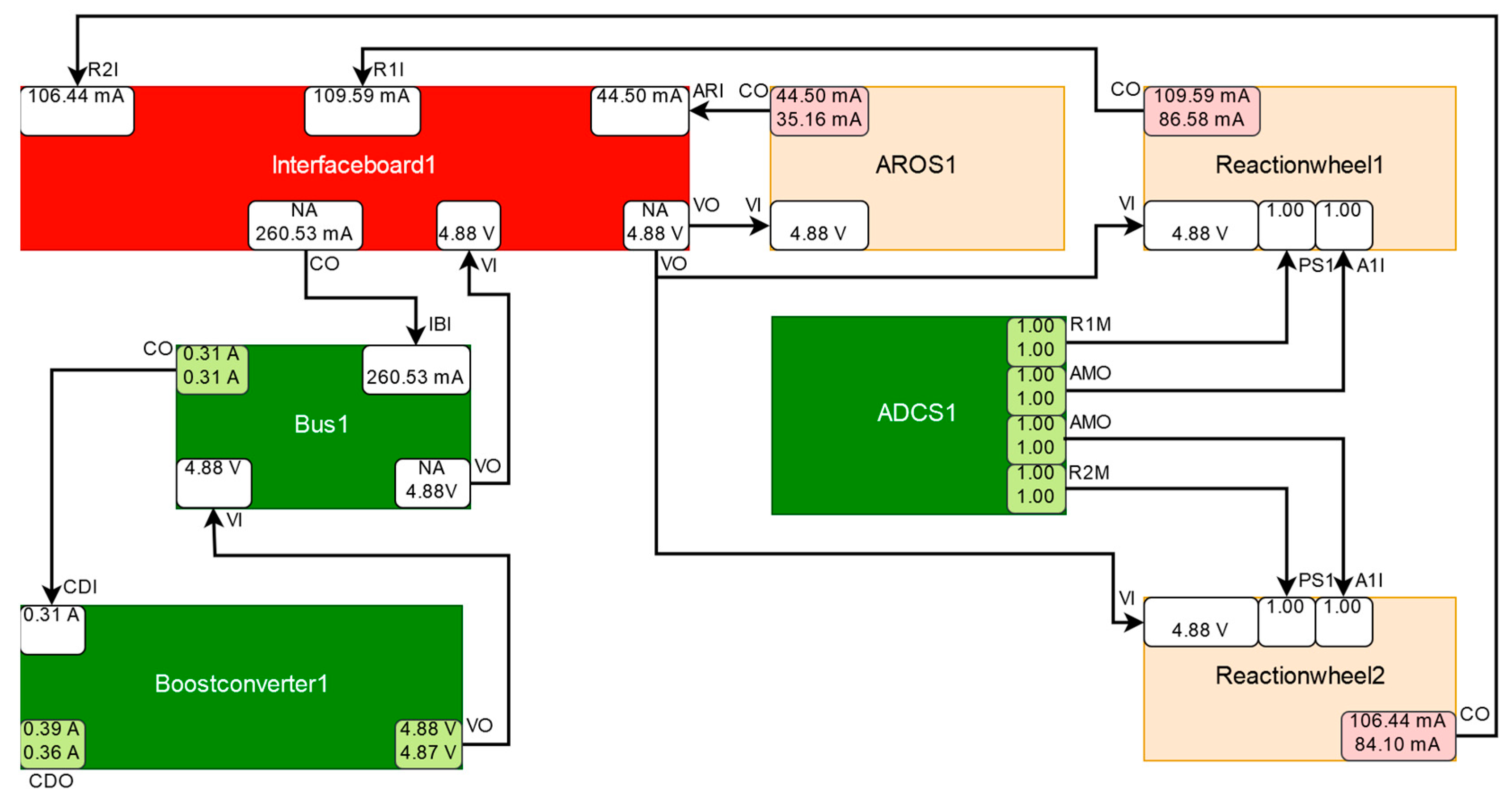
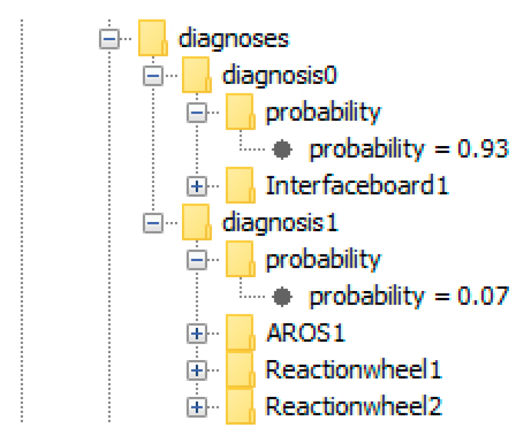
5.5. Interface Board Malfunction
5.6. Summary of Results
6. Discussion
7. Conclusions
Author Contributions
Funding
Conflicts of Interest
References
- Shim, D.; Yang, C. Optimal Configuration of Redundant Inertial Sensors for Navigation and FDI Performance. Sensors 2010, 10, 6497–6512. [Google Scholar] [CrossRef]
- Bouallègue, W.; Bouslama Bouabdallah, S.; Tagina, M. Causal approaches and fuzzy logic in FDI of Bond Graph uncertain parameters systems. In Proceedings of the IEEE International Conference on Communications, Computing and Control Applications (CCCA), Hammamet, Tunisia, 3–5 March 2011. [Google Scholar]
- Venkatasubramanian, V.; Rengaswamy, R.; Yin, K.; Kavuri, S. A review of process fault detection and diagnosis: Part I: Quantitative model-based methods. Comput. Chem. Eng. 2003, 27, 293–311. [Google Scholar] [CrossRef]
- Thirumarimurugan, M.; Bagyalakshmi, N.; Paarkavi, P. Comparison of fault detection and isolation methods: A review. In Proceedings of the 2016 10th International Conference on Intelligent Systems and Control (ISCO), Coimbatore, India, 7–8 January 2016. [Google Scholar] [CrossRef]
- Patton, R.; Uppal, F.; Simani, S.; Polle, B. Robust FDI applied to thruster faults of a satellite system. Control Eng. Pract. 2010, 18, 1093–1109. [Google Scholar] [CrossRef]
- Falcoz, A.; Henry, D.; Zolghadri, A. Robust Fault Diagnosis for Atmospheric Reentry Vehicles: A Case Study. IEEE Trans. Syst. Man Cybern. Part A Syst. Hum. 2010, 40, 886–899. [Google Scholar] [CrossRef]
- Reiter, R. A theory of diagnosis from first principles. Artif. Intell. 1987, 32, 57–95. [Google Scholar] [CrossRef]
- de Kleer, J.; Williams, B. Diagnosing multiple faults. Artif. Intell. 1987, 32, 97–130. [Google Scholar] [CrossRef]
- Fellinger, G.; Dietrich, G.; Fette, G.; Kayal, H.; Puppe, F.; Schneider, V.; Wojtkowiak, H. ADIA: A Novel Onboard Failure Diagnostic System for Nanosatellites. In Proceedings of the 64th International Astronautical Congress 2013, Beijing, China, 23–27 September 2013. [Google Scholar]
- Picardi, C. A Short Tutorial on Model-Based Diagnosis. 2005. Available online: https://pdfs.semanticscholar.org/e3e7/fbf0581d05aeff0e213641f5b36886264dbd.pdf?_ga=2.250857024.778130362.1569288585-1114982217.1569288585 (accessed on 7 August 2019).
- De Kleer, J.; Kurien, J. Fundamentals of model-based diagnosis. In Proceedings of the Fifth IFAC Symposium on Fault Detection, Supervision and Safety of Technical Processes (Safeprocess), Washington, DC, USA, 23–27 June 2003. [Google Scholar]
- De Kleer, J.; Mackworth, A.; Reiter, R. Characterizing diagnoses and systems. Artif. Intell. 1992, 56, 197–222. [Google Scholar] [CrossRef]
- Fröhlich, S. Model-Based Error Detection and Diagnostics in Real Time Using the Example of a Fuel Cell (Modellbasierte Fehlererkennung und Diagnose in Echtzeit am Beispiel einer Brennstoffzelle). Ph.D. Thesis, University of Kassel, Kassel, Germany, 2009. [Google Scholar]
- Dang Duc, N. Conception and Evaluation of a Hybrid, Scalable Tool for Mechatronic System Diagnostics Using the Example of a Diagnostic System for Independent Garages (Konzeption und Evaluation eines Hybriden, Skalierbaren Werkzeugs zur Mechatronischen Systemdiagnose am Beispiel eines Diagnosesystems für freie Kfz-Werkstätten). Ph.D. Thesis, University of Würzburg, Würzburg, Germany, 2011. [Google Scholar]
- Dang Duc, N.; Engel, P.; de Boer, G.; Puppe, F. Hybrid, scalable diagnostic system for independent garages (Hybrides, skalierbares Diagnose-System für freie Kfz-Werkstätten). Artif. Intell. 2009, 23, 31–37. [Google Scholar]
- Williams, B.C.; Nayak, P.P. A model-based approach to reactive self-configuring systems. In Proceedings of the Thirteenth National Conference on Artificial Intelligence (AAAI-96), Portland, OR, USA, 4–8 August 1996. [Google Scholar]
- Hayden, S.; Sweet, A.; Shulman, S. Lessons learned in the Livingstone 2 on Earth Observing One flight experiment. In Proceedings of the Infotech@Aerospace, Arlington, VA, USA, 26–29 September 2005. [Google Scholar]
- Sweet, A.; Bajwa, A. Lessons Learned from Using a Livingstone Model to Diagnose a Main Propulsion System. In Proceedings of the JANNAF 39th CS/27th APS/21st PSHS/3rd MSS Joint Subcommittee Meeting, Colorado Springs, CO, USA, 1–5 December 2003. [Google Scholar]
- Kolcio, K. Model-Based Fault Detection and Identification System for Increased Autonomy. In Proceedings of the AIAA SPACE 2016, Long Beach, CA, USA, 13–16 September 2016. [Google Scholar]
- Cordier, M.; Dague, P.; Levy, F.; Montmain, J.; Staroswiecki, M.; Trave-Massuyes, L. Conflicts versus Analytical Redundancy Relations: A Comparative Analysis of the Model Based Diagnosis Approach from the Artificial Intelligence and Automatic Control Perspectives. IEEE Trans. Syst. Man Cybern. Part B (Cybern.) 2004, 34, 2163–2177. [Google Scholar] [CrossRef]
- Kayal, H.; Balagurin, O.; Djebko, K.; Fellinger, G.; Puppe, F.; Schartel, A.; Schwarz, T.; Vodopivec, A.; Wojtkowiak, H. SONATE—A Nano Satellite for the in-Orbit Verification of Autonomous Detection, Planning and Diagnosis Technologies. In Proceedings of the AIAA SPACE 2016, Long Beach, CA, USA, 13–16 September 2016. [Google Scholar]
- Fellinger, G.; Djebko, K.; Jäger, E.; Kayal, H.; Puppe, F. ADIA++: An Autonomous Onboard Diagnostic System for Nanosatellites. In Proceedings of the AIAA SPACE 2016, Long Beach, CA, USA, 13–16 September 2016. [Google Scholar]
- Havelka, T.; Stumptner, M.; Wotawa, F. AD2L-A Programming Language for Model-Based Systems (Preliminary Report). In Proceedings of the Eleventh International Workshop on Principles of Diagnosis (DX-00), Morelia, Mexico, 8–10 June 2000. [Google Scholar]
- Fleischanderl, G.; Havelka, T.; Schreiner, H.; Stumptner, M.; Wotawa, F. DiKe—A Model-Based Diagnosis Kernel and Its Application. In Proceedings of the KI 2001: Advances in Artificial Intelligence, Vienna, Austria, 19–21 September 2001; pp. 440–454. [Google Scholar] [CrossRef]
- Koitz, R.; Wotawa, F. SAT-Based Abductive Diagnosis. In Proceedings of the 26th International Workshop on Principles of Diagnosis, Paris, France, 31 August–3 September 2015. [Google Scholar]
- Zhao, X.; Zhang, L.; Ouyang, D.; Jiao, Y. Deriving all minimal consistency-based diagnosis sets using SAT solvers. Prog. Nat. Sci. 2009, 19, 489–494. [Google Scholar] [CrossRef]
- Pill, I.; Quaritsch, T.; Wotawa, F. From conflicts to diagnoses: An empirical evaluation of minimal hitting set algorithms. In Proceedings of the 22nd International Workshop on Principles of Diagnosis (DX-2011), Murnau, Germany, 4–7 October 2011. [Google Scholar]
- Greiner, R.; Smith, B.; Wilkerson, R. A correction to the algorithm in reiter’s theory of diagnosis. Artif. Intell. 1989, 41, 79–88. [Google Scholar] [CrossRef]
- Djebko, K.; Fellinger, G.; Puppe, F.; Kayal, H. Cyclic Genetic Algorithm for High Quality Automatic Calibration of Simulation Models with an Use Case in Satellite Technology. Int. J. Model. Simul 2019. under review. [Google Scholar]
- Holland, J. Adaptation in Natural and Artificial Systems; University of Michigan Press: Ann Arbor, MI, USA, 1975. [Google Scholar]
- Russel, S.; Norvig, P. Artificial Intelligence: A Modern Approach, 3rd ed.; Prentice Hall: Upper Saddle River, NJ, USA, 2009. [Google Scholar]


| Component | Instances | Description |
|---|---|---|
| Battery | 2 | A battery pack consisting of 4 single batteries. The main power source of the satellite. |
| Solarpanel | 4 | A single solar panel, explicitly modelled as a sensor component |
| Boostconverter | 2 | The PCUs boost converter is used to generate a stable bus voltage. Since most consumers need a voltage higher, than the main power supply can provide, each of the two power supply busses uses one of these converters. |
| Bus | 2 | The power supply bus is used to connect the consumers to the main power supply via a boost converter. |
| Magnetorquer | 2 | The magnetorquer component combines three actual magnetorquers. A ferrite core coil (X-direction) and two air core coils (Y- and Z- direction) are used. |
| Terminationboard | 2 | Connects three single physical magnetorquers in either positive or negative X-, Y-, Z-direction to a power supply bus. |
| Reactionwheel | 3 | A single experimental reaction wheel. |
| ASAP | 1 | The ASAP-payload. |
| AROS | 2 | The AROS-payload. |
| Interfaceboard1 | 1 | Connects two reaction wheels, an AROS unit and ASAP to a power supply bus. |
| Interfaceboard2 | 1 | Connects a reaction wheel, an AROS unit and ASAP to a power supply bus. |
| ADCSConv | 2 | The voltage converter of the attitude determination and control system. |
| ADCS | 2 | The attitude determination and control system. |
| Magnetometer | 4 | The magnetometer of the ADCS. |
| Gyro | 4 | The gyro of the ADCS. |
| Transceiver | 2 | The transceiver of the satellite. |
| HISPICO | 2 | A single HISPICO device. |
| SSTV | 2 | A SSTV device. |
| PCU | 2 | The dedicated microcontroller of the PCU. |
| ADIA | 2 | The ADIA-payload. |
| OBDHConv | 4 | The voltage converter of the on board computer. |
| OBDH | 4 | The on board computer of the satellite. |
| SunSensor | 1 | The SunSensor component combines 12 actual sun sensors. |
| Ex. | Malfunctioning Components | Detected Discrepancies | Identified Diagnoses (Probability) | Result |
|---|---|---|---|---|
| 1 | Boostconverter2 | CDO at Boostconverter2 | Boostconverter2 (100%) | Cause of discrepancy correctly diagnosed. |
| 2 | Transceiver1 | CO at Transceiver1 | Transceiver1 (100%) | Cause of discrepancy correctly diagnosed. |
| 3 | OBDH1Conv | VO at OBDH1Conv | OBDH1Conv (100%) | Cause of discrepancy correctly diagnosed. |
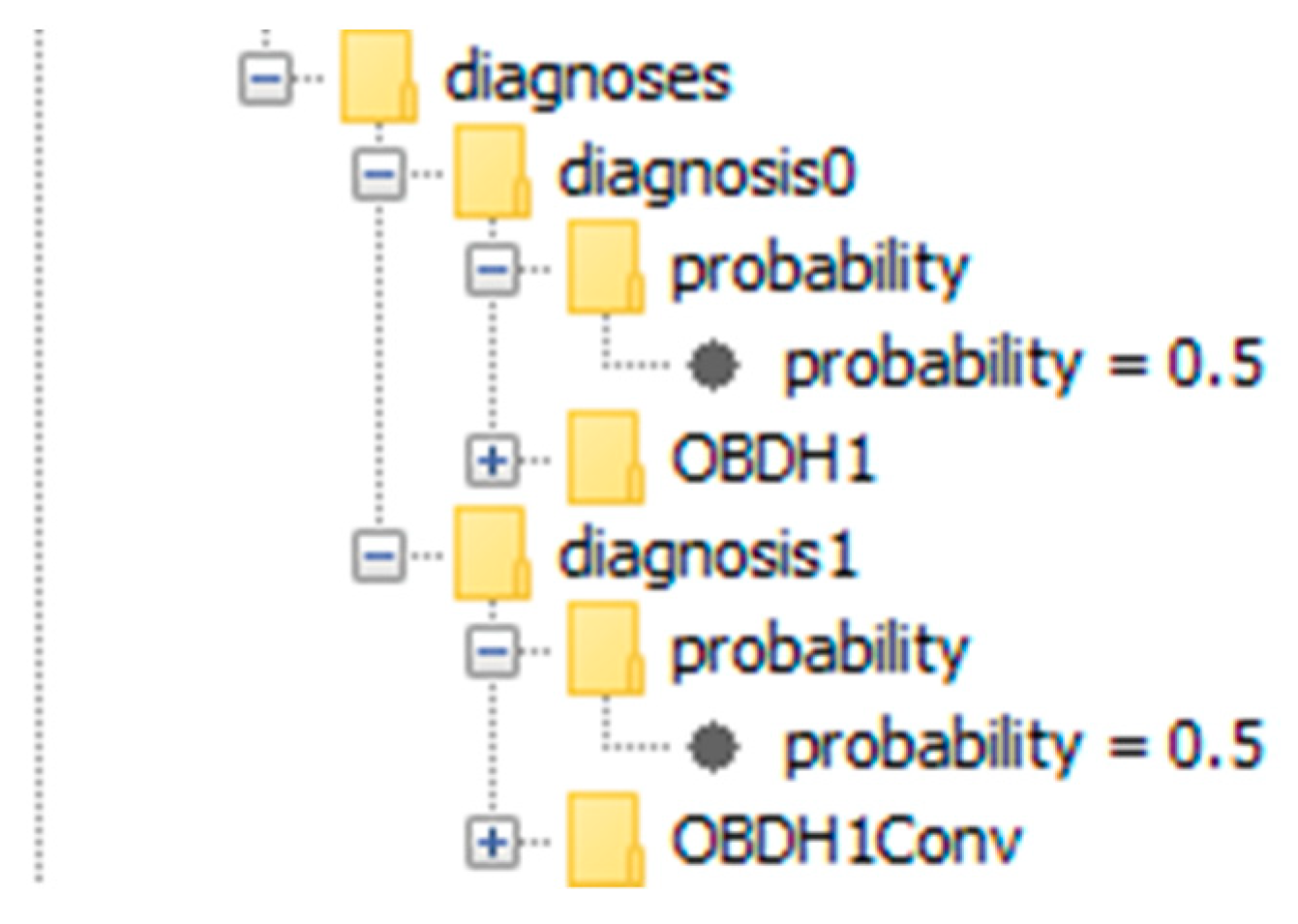
| 4 | OBDH1Conv | VO at OBDH1Conv, CO at OBDH1 | OBDH1Conv (50%)/OBDH1 (50%) | Both discrepancies detected. Cyclical relationship identified and most viable diagnoses computed. |
| 5 | Interfaceboard1 | CO at AROS1, CO at Reactionwheel1, CO at Reactionwheel2 | Interfaceboard1 (93%)/AROS1, Reactionwheel1, Reactionwheel2 (7%) | Discrepancies caused by not directly observable malfunction detected. Root cause determined and plausible probabilities assigned to diagnoses. |
© 2019 by the authors. Licensee MDPI, Basel, Switzerland. This article is an open access article distributed under the terms and conditions of the Creative Commons Attribution (CC BY) license (http://creativecommons.org/licenses/by/4.0/).
Share and Cite
Djebko, K.; Puppe, F.; Kayal, H. Model-Based Fault Detection and Diagnosis for Spacecraft with an Application for the SONATE Triple Cube Nano-Satellite. Aerospace 2019, 6, 105. https://doi.org/10.3390/aerospace6100105
Djebko K, Puppe F, Kayal H. Model-Based Fault Detection and Diagnosis for Spacecraft with an Application for the SONATE Triple Cube Nano-Satellite. Aerospace. 2019; 6(10):105. https://doi.org/10.3390/aerospace6100105
Chicago/Turabian StyleDjebko, Kirill, Frank Puppe, and Hakan Kayal. 2019. "Model-Based Fault Detection and Diagnosis for Spacecraft with an Application for the SONATE Triple Cube Nano-Satellite" Aerospace 6, no. 10: 105. https://doi.org/10.3390/aerospace6100105
APA StyleDjebko, K., Puppe, F., & Kayal, H. (2019). Model-Based Fault Detection and Diagnosis for Spacecraft with an Application for the SONATE Triple Cube Nano-Satellite. Aerospace, 6(10), 105. https://doi.org/10.3390/aerospace6100105