Article

Effects of Nozzle Pressure Ratio and Nozzle-to-Plate Distance to Flowfield Characteristics of an Under-Expanded Jet Impinging on a Flat Surface

Thermal-Hydraulic Research Laboratory, Department of Nuclear Engineering, Texas A& M University, College Station, TX 77845, USA
*
Author to whom correspondence should be addressed.
Aerospace 2019, 6(1), 4; https://doi.org/10.3390/aerospace6010004
Submission received: 2 December 2018 / Revised: 27 December 2018 / Accepted: 4 January 2019 / Published: 6 January 2019
(This article belongs to the Special Issue Under-Expanded Jets)

Abstract

:
The current work experimentally investigates the flowfield characteristics of an under-expanded turbulent jet impinging on a solid surface for various nozzle-to-plate distances 2.46 D j , 1.64 D j , and 0.82 D j ( D j is the jet hydraulic diameter), and nozzle pressure ratios (NPRs) ranging from 2 to 2.77 . Planar particle image velocimetry (PIV) measurements were performed in the central plane of the test nozzle and near the impingement surface. From the obtained PIV velocity vector fields, flow characteristics of under-expanded impinging jets, such as mean velocity, root-mean-square fluctuating velocity, and Reynolds stress profiles, were computed. Comparisons of statistical profiles obtained from PIV velocity measurements were performed to study the effects of the impingement surface, nozzle-to-plate distances, and NPRs to the flow patterns. Finally, proper orthogonal decomposition (POD) analysis was applied to the velocity snapshots to reveal the statistically dominant flow structures in the impinging jet regions.

Graphical Abstract

1. Introduction

The impinging jet configuration has received many considerations from researchers due to its widespread use in many industrial applications. For example, the impinging jets can be used for cooling of hot surfaces such as turbine blade (Saddington et al. [1], Hadžiabdić and Hanjalić [2]), as rocket engine or vertical and short take off and landing aircraft (Krothapalli et al. [3], Cabrita et al. [4], Saddington et al. [5,6], Wilke and Sesterhenn [7]), and as torque generator in turbomachinery system.
The flow characteristics of impinging jets, despite the geometrical simplicity, are very complex and have posed challenges to numerical simulations, particularly for turbulence modelling (Hadžiabdić and Hanjalić [2]). The jet flow configurations discussed in this paper are under-expanded, subsonic and supersonic free jets, i.e., jets exhaust in a quiet medium, and jets impinging on a solid surface, that are commonly found in aerospace engineering applications and turbomachinery systems. An under-expanded jet may occur when the jet nozzle releases a fluid at a pressure greater than the ambient pressure. A comprehensive review of free under-expanded jets can be seen in Franquet et al. [8]. The flow configuration of supersonic impinging jet has rich and complex flow structures (Henderson [9]) that are originated from the compressibility and turbulent flows (Weightman et al. [10]). Besides, the supersonic impinging jet is a highly resonant flowfied that is governed by a well-known aeroacoustics feedback loop (Weightman et al. [10], Uzun et al. [11], Akamine et al. [12]). The feedback loop initiates as instability waves in the jet shear layer, then grow into large-scale vortices as they travel downstream (Brown and Roshko [13], Tam and Ahuja [14], Henderson and Powell [15]). The impact of the large-scale vortices on the solid surface produces pressure fluctuations and acoustic waves propagating upstream (Krothapalli et al. [3], Henderson [16], Henderson et al. [17], Sinibaldi et al. [18], Gojon et al. [19]). These upstream propagated waves reach the nozzle outlet and generate the instability waves, closing the feedback loop (Henderson and Powell [15], Ho and Nosseir [20], Nosseir and Ho [21]).
In the current communication, we experimentally study the under-expanded turbulent impinging jets featuring in many important applications of turbomachinery and aerospace engineering. Particularly, the test model is a convergence-divergence nozzle, which is typically installed in turbomachinery systems of many power plants in United States. When in operation, the nozzle will exhaust gas (air and/or steam) to the turbine blades and induce rotations for the turbomachinery shaft. It should be noted that at this stage, the flow configuration presented in this paper is unheated, under-expanded air jets impinging on a flat surface that can be considered as a simplified version of the practical system. Nevertheless, it is still a valuable benchmark to gain a proper understanding of the flow mixing between the subsonic and supersonic jet flows and an ambient surrounding fluid with and without the presence of the impinging surface.
Researchers at Texas A&M University have conducted isothermal velocity measurements of subsonic and supersonic under-expanded free jets and impinging jets. The general purpose of these tests is to perform high-spatial resolution measurements of the velocity fields for different flow configurations of under-expanded jets. The experimental activities provide an experimental database of velocity measurements suitable for validating system-level codes and developing the computational fluid dynamics (CFD) models that are currently considered for subsonic and supersonic jet flows.
The objective of our study is to investigate the flow characteristics of under-expanded turbulent jets impinging on a solid surface with various nozzle pressure ratios (NPRs) ranging from 2 to 2.77 , and different values of nozzle-to-plate gaps. These spatial distances are e = 10 (mm), 20 (mm), and 30 (mm), that are typical in the practical turbomachinery systems. The resulted non-dimensional gap spacings, defined as e / D j ( D j is the jet hydraulic diameter), are 0.82 , 1.64 , and 2.46 , respectively. The flowfield characteristics in the central plane of the test nozzle and near the impingement surface are obtained by using the two-dimensional two-component (2D2C) particle image velocimetry (PIV) technique. The PIV measurements will provide the full-field flow characteristics of the flow mixing between the under-expanded free jets, impinging jets and surrounding areas. The obtained experimental results at high-spatial resolutions can be then used for validation of theoretical and CFD models, and for providing technical supports to the system design. The structure of this paper is as followed. The experimental facility of impinging jet configuration and PIV experimental setup to acquire the velocity are presented in Section 2. From the obtained PIV velocity vector fields corresponding to various spatial gaps and NPRs, statistical results including the first- and second-order flow statistics, such as mean velocity, root-mean-square fluctuating velocity and Reynolds stress, are discussed in Section 3. Effects of the impingement surface and NPRs to the flow patterns and comparisons of statistical profiles are discussed in Section 3.2. Finally, proper orthogonal decomposition (POD) analysis is applied to reveal the statistically dominant flow structures that play important roles to the flow dynamics and acoustic characteristics of impinging jets. Results from the velocity decomposition are discussed in Section 4, followed by the conclusions in Section 5.

2. Experimental Facility and Particle Image Velocimetry (PIV) Experimental Setup

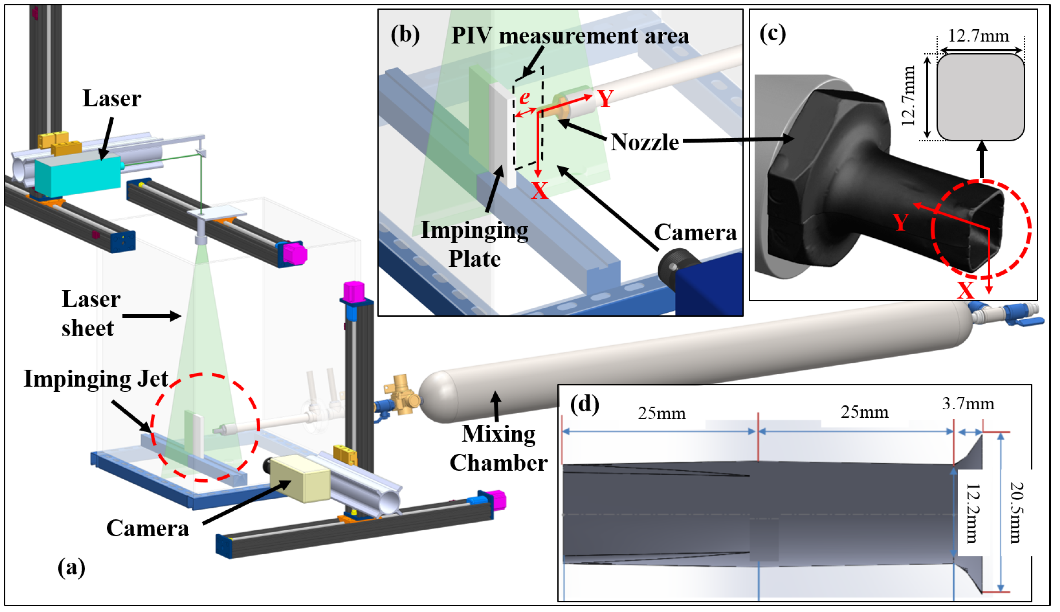
2.1. Experimental Facility of Impinging Jet

In this section, we describe the experimental facility of an under-expanded turbulent jet impinging on a solid surface. Figure 1a shows the experimental rig, while Figure 1b illustrates the PIV experimental setup, and Figure 1c,d depict a close-view and dimensions of the test nozzle used in this study. It is noted that the test model is a convergence-divergence nozzle, which has been removed from a turbomachinery system used in a power plant. The test nozzle, therefore, had few minor geometrical distortions due to mechanical stresses from the installation, maintenance and operating conditions of the system. The jet nozzle had a throat diameter of 12.2 mm, a square cross-section outlet with rounded edges, and an overall length of 50 mm as shown in Figure 1c,d. The hydraulic diameter of the test nozzle was estimated using the throat diameter D j = 12.2 (mm).
The governing parameters of an under-expanded turbulent jet impinging on a surface are the nozzle pressure ratio (NPR), defined as N P R = p e x i t / p a m b , in which p e x t and p a m b are the pressures of the jet exit and ambient air, D j is the nozzle hydraulic diameter, and e is the nozzle-to-plate distance (Henderson [9], Ho and Nosseir [20]). The experimental test rig consisted of a cylindrical mixing chamber with an internal diameter of 152.4 mm and a length of 1778 mm. The mixing chamber was placed horizontally and its inlet was connected to a laboratory air compressor. For the experiments considered here, this source of compressed air (100 psi) was capable of maintaining a constant inlet flow rate and pressure throughout each time. The air flow rate was controlled manually using a ball valve and a pressure regulator. The compressed air was accumulated in the mixing chamber, whose pressure was adjusted using a pressure regulator maintaining the pressure at the jet exit, p e x i t . The mixing chamber was instrumented with a thermocouple and a pressure transducer that were connected to a National Instrument Data Acquisition system to provide information on the stagnation conditions. The outlet of the mixing chamber was attached to a circular pipe with a length of 914.4 mm and a diameter of 19.05 mm, and the test nozzle. The pipe length was chosen so that it exceeded 10 hydraulic diameters of the nozzle to ensure fully developed turbulent flow at the nozzle exit (Kays [22], Solovitz et al. [23]).

2.2. PIV Experimental Setup

Figure 1 illustrates the experimental setup of two-dimensional two-component (2D2C) PIV measurements of the impinging jet flow configuration. For the current PIV measurements, the measured flow area was illuminated by the laser sheet and located at the center plane of the test nozzle, as shown in Figure 1b. The origin of the coordinate system was at the center of the nozzle exit, in which, x-direction is normal to the jet centerline, and negative y-direction is the jet axis. The jet Reynolds number is defined as
R e j = V j D j / ν ,
in which, V j is the jet velocity at the nozzle outlet, D j is the jet hydraulic diameter, and ν is the kinematic viscosity of air. The velocity components corresponding to the x and y directions were U and V for the time-averaged velocity, and u and v for the fluctuating velocity, respectively. In this paper, velocity measurements in the central plane of the test nozzle for the configurations of under-expanded free jets and impinging jets with various nozzle-to-plate gaps e = 10 mm, 20 mm, and 30 mm, are discussed.
The 2D2C PIV system consisted of a dual-head Nd:YAG laser, a digital charge couple device (CCD) camera, a synchronizer, and a computer. Each laser beam of the double-pulsed laser was capable of 200 mJ at a wavelength of 532 nm. These beams were adjusted by using an optical system of cylindrical and spherical lenses to form a 1-mm-thick laser sheet. For all the experiments, the laser sheet was positioned at the central plane of the test nozzle. For the current experimental configurations, it is expected that the impinging jet possessed three-dimensional flow structures that produced particle displacements perpendicular to the laser sheet (Nguyen et al. [24], Nguyen and Souad [25]). For the 2D2C PIV measurements, these out-of-plane particle displacements could make the loss of pairs significant, which could strongly reduce the correlation peaks computed from image cross-correlation calculations, and then reduce the possibility of searching a valid peak from the correlation map. To mitigate this difficulty, we followed suggestions of Raffel et al. [26] to choose an appropriate laser sheet thickness and the time interval between the image recordings to accommodate the out-of-plane displacements of particles. The laser sheet thickness of 1 mm was therefore optimized to be thin enough to guarantee an adequate particle image intensity but thick enough to reduce the loss of image pairs due to out-of-plane particle displacements. The PIV double-pulsed image pairs were acquired using the CCD camera 4MP, which had a maximum resolution of 2336 × 1752 and a pixel size of 5.5 × 5.5 μ m 2 , at a sampling rate of 15 Hz. The Zeiss camera lens had a 105-mm focal length and an f/5.6 aperture. A droplet generator was used with Di-Ethyl-Hexyl-Sebacat liquid to generate particles with a mean diameter of 1 μ m to seed the inlet of the mixing chamber and the jet. Depending on the estimated jet velocity for various NPRs, the time intervals between the first and second image exposures varied from 3 μ s to 1 μ s, yielding maximum particle displacements of 45 pixels. For velocity measurements of high-speed flows using laser-based techniques, Scarano [27], Alvi et al. [28], and Mitchell et al. [29] discussed the importance of seeding particles because particle lag could occur in flow regions of very high velocity gradients, such as shock waves and wall jets. Following the discussions in Raffel et al. [26] and in the study of Sinibaldi et al. [18], particle response to a constant flow acceleration is defined by
τ p = d p 2 ρ p 18 μ
where d p and ρ p are the diameter and density of the seeding particle, and μ is the dynamic viscosity of the air. The Stokes number ( S t k ) is defined as the ratio between the particle relaxation time τ p and the characteristics flow timescale τ f . Samimy and Lele [30] suggested an estimation of the flow timescale by assuming the particle maximum slip velocity as V j (Sinibaldi et al. [18]), as follow
τ f = 10 D j V j .
The seeding particles can be considered to follow the flow properly if the particle relaxation time τ p is much smaller than the flow timescale τ f , i.e., Stokes number S t k 1 (Erdem et al. [31], Ragni et al. [32]). Providing the properties of the DEHS particles, air properties, and jet velocity for each experimental measurement in the current study, one can obtain the particle response time is τ p = 2.82 × 10 6 s and τ f = 3.81 × 10 4 s. This yields the Stokes number S t k 0.031 , thus ensuring reliable fluid flow detection based on the seeding particles and laser illumination (Sinibaldi et al. [18]). Table 1 shows typical flow conditions calculated at the nozzle exit for the free jets and impinging jets at various nozzle-to-plate gaps and various values of NPRs.
For the specific values of NPRs and spatial gaps between the nozzle and impinging plane, sequences of image pairs, ranging from 350 to 1600 pairs, were recorded during multiple experimental runs. All 12-bit depth PIV double-exposure images were processed by the advanced multi-pass, multi-grid robust phase correlation (RPC) algorithms (Eckstein et al. [33], Eckstein and Vlachos [34]). The PIV image processing had four iterations, which started from 196 × 196 pixels and ended at 32 × 32 pixels, respectively. Particle displacements initially calculated from the previous iteration were used to shift the interrogation window in the next iteration. All PIV iterations had a 50 % window overlap, yielding the final spatial gap between two adjacent vectors of 0.3 mm. In all the PIV iterations, particle displacements were computed from the correlation map with a Gaussian peak fit for sub-pixel accuracy (Raffel et al. [26]). Within each iteration, statistical validations were performed to identify and replace erroneous vectors. We applied the median filter, proposed by Westerweel [35], and used the standard deviations of the neighboring vectors to filter out spurious vectors. The resulted blanks were then filled by velocity interpolation. For all the tests presented in this paper, the percentage of erroneous vectors, which were defined as the numbers of vectors failed the validation process in the final iteration, and averaged over the number of velocity snapshots, was less then 5 % . The overall uncertainty in the PIV velocity measurements was estimated approximately 0.1 pixels, yielding less than 1 % to 2 % of the mean jet velocity. Performance and uncertainty of the PIV post-processing using RPC algorithm were evaluated in studies of Timmins et al. [36], Wilson and Smith [37], Charonko and Vlachos [38], and Boomsma et al. [39].

3. Results from PIV Measurements of Under-Expanded Free Jets and Impinging Jets

The collections of PIV experimental images were processed, and the obtained PIV velocity vectors were used to compute the flow statistics for various configurations of free jet and impinging jet. In this section, we present the first-order statistics, i.e., mean velocity, and second-order flow statistics, such as root-mean-square (RMS) fluctuating velocity, Reynolds stress, and turbulent kinetic energy, computed for the configurations of free jets and impinging jets with various nozzle-to-plate distances of e = 30 mm, 20 mm, and 10 mm. In addition, statistical results corresponding to different values of NPRs, i.e., N P R 1 = 2 , N P R 2 = 2.2 , N P R 3 = 2.5 , and N P R 4 = 2.77 , are compared. From the obtained instantaneous 2D2C PIV velocity vector fields, the flow statistics, including mean velocity, RMS fluctuating velocity, Reynolds stress and turbulent kinetic energy, are calculated as follows. The mean velocity components U and V are computed as
U = 1 N i = 1 N u i V = 1 N i = 1 N v i ,
and the RMS fluctuating velocities, u r m s and v r m s , and Reynolds stress, u v , are calculated as
u r m s = 1 N i = 1 N u i 2 v r m s = 1 N i = 1 N v i 2 u v = 1 N i = 1 N u i U v i V .
Because the current 2D2C PIV measurements were able to measure two velocity components, turbulent kinetic energy, k, is computed as
k = 1 2 N i = 1 N u i 2 + v i 2 .
In Equations (4)–(6), u and v are the instantaneous velocity components along x and y directions, u and v are the fluctuating velocity components, and N is the number of instantaneous velocity snapshots.

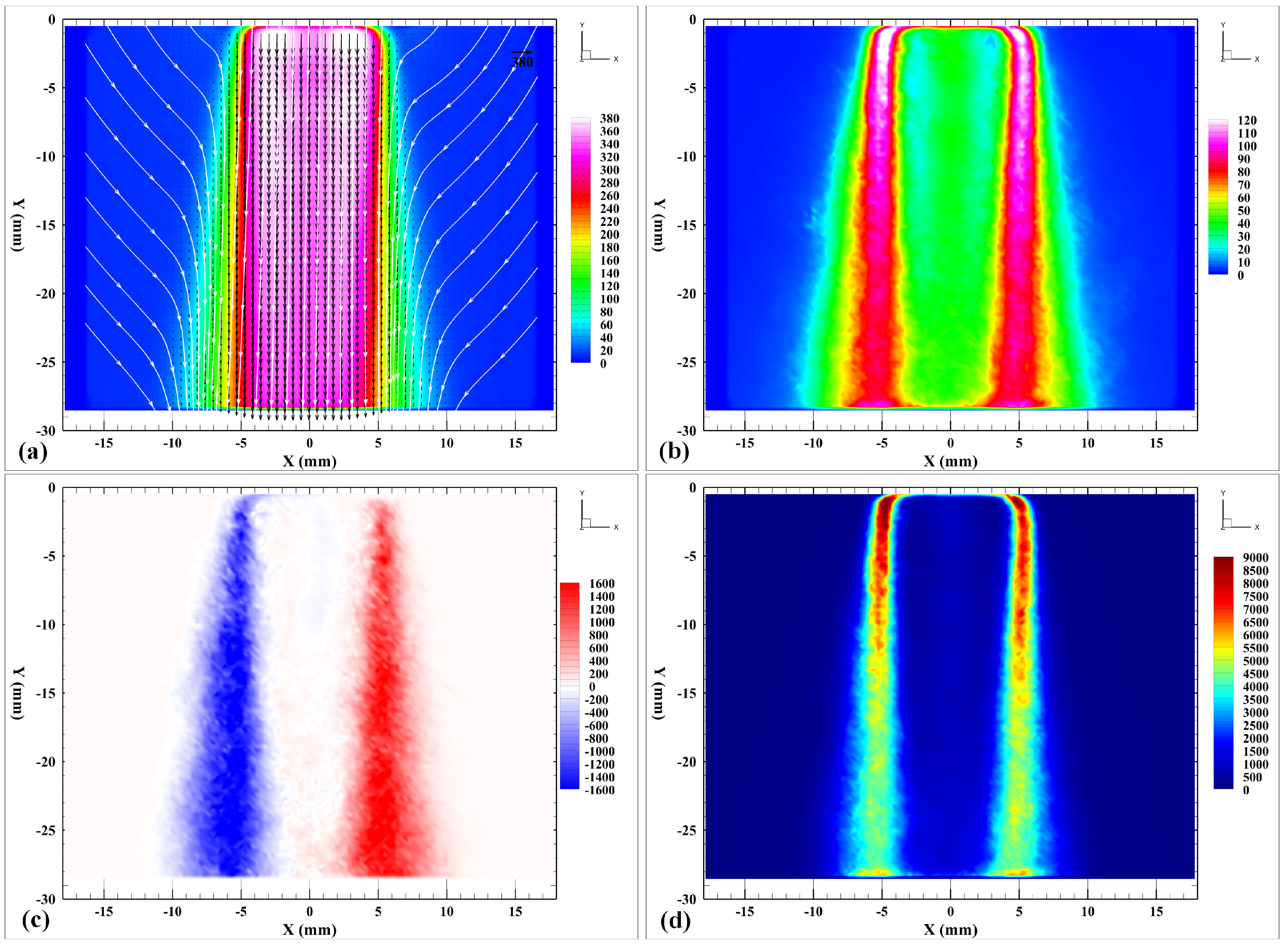
3.1. Experimental Results of Under-Expanded Free Jets for Various Values of NPRs

For the free jet configuration, velocity measurements were performed on the center plane of the test nozzle without the presence of the impingement surface for various NPRs. Figure 2 illustrates the results obtained from the 2D2C PIV measurements of the free jet for N P R 4 = 2.77 . These are the mean in-plane velocity vectors and color contour of velocity magnitude, color contours of RMS fluctuating axial velocity v r m s , Reynolds stress u v , and turbulent kinetic energy k. The color contours illustrated the near-field zone of the under-expanded jet. The near-field zone can be divided into two regions, i.e., the core region and the mixing layer (Franquet et al. [8]). The core region is separated from the surround fluid region and its characteristics are expressed by the compressible effects. In the mixing layer, the flow entrainment between the discharged fluid and the surrounding region is characterized by vortical flow structures. Color contour of velocity magnitude depicted that the jet core region was at supersonic up to approximately 1 D j . Contours of RMS fluctuating velocity v r m s and turbulent kinetic energy k showed the jet shear layers formed between the core region and surrounding flow region. Besides, color contour of Reynolds stress, u v , illustrated the development of the mixing layer in the downstream direction.
In Figure 3, the first- and second-order flow statistics, such as mean velocity, RMS fluctuating axial velocity, Reynolds stress and turbulent kinetic energy obtained along three lines, i.e., Line 1 ( y = 2.54 ) mm, Line 2 ( y = 12.7 ) mm, and Line 3 ( y = 25.4 ) mm, were compared. In the comparisons, the mean axial velocity, V, and RMS fluctuating axial velocity v r m s , were normalized by the sonic velocity c, while the Reynolds stress, u v , and turbulent kinetic energy, k, were normalized by c 2 .
In the comparison of normalized mean axial velocity, V / c , it can be seen that velocity profiles for N P R 1 and N P R 2 had their maximum values along the jet centerline. On the other hand, velocity profiles for N P R 3 and N P R 4 near the nozzle exit (Line 1) showed the maximum velocity along the nozzle perimeter. For N P R 3 and N P R 4 , the mean axial velocities obtained at the nozzle exit were 343 m/s and 353 m/s, respectively, which were greater than sonic velocity c. This phenomenon indicated that the jet flows at higher NPRs expanded to atmospheric pressure and experienced the shock in vicinity of the nozzle exit. For all the values of NPRs, the jet velocities along the center line reduced further downstream, and only profiles of V / c at high NPRs showed the maximum peaks along the jet perimeter. The mean axial velocity outside the jet core reduced gradually and became flatter in the region further downstream, indicating the entrainment mechanisms outside the jet. For the low-speed cases of under-expanded free jet, the maximum jet velocity is along the centerline, the flow entrainment was driven by the centerline jet velocity, which transferred the flow energy to the turbulent eddies in the jet shear layers (Saffaraval and Solovitz [40]). For the high-speed cases, the jet velocity remained supersonic in the core region while on either side, the surrounding velocity is subsonic.
In Figure 3b, profiles of normalized RMS fluctuating axial velocity v r m s / c for N P R 1 and N P R 2 had two local peaks on both sides of the jet flows around X / D j = 0.33 to 0.36 , while profiles of v r m s / c for N P R 3 and N P R 4 had two local peaks at X / D j = 0.4 and an additional local peak at X / D j = 0 . Similar observations can also be seen in profiles of turbulent kinetic energy, k / c 2 . The appearances of additional peaks at X / D j = 0 in the profiles of v r m s / c and k / c 2 can be attributed by the formation of shock cell at a higher-pressure ratio N P R 4 . It is noted that profiles of Reynolds stress, u v / c 2 obtained for N P R 3 and N P R 4 revealed very low turbulence levels in the jet core region.

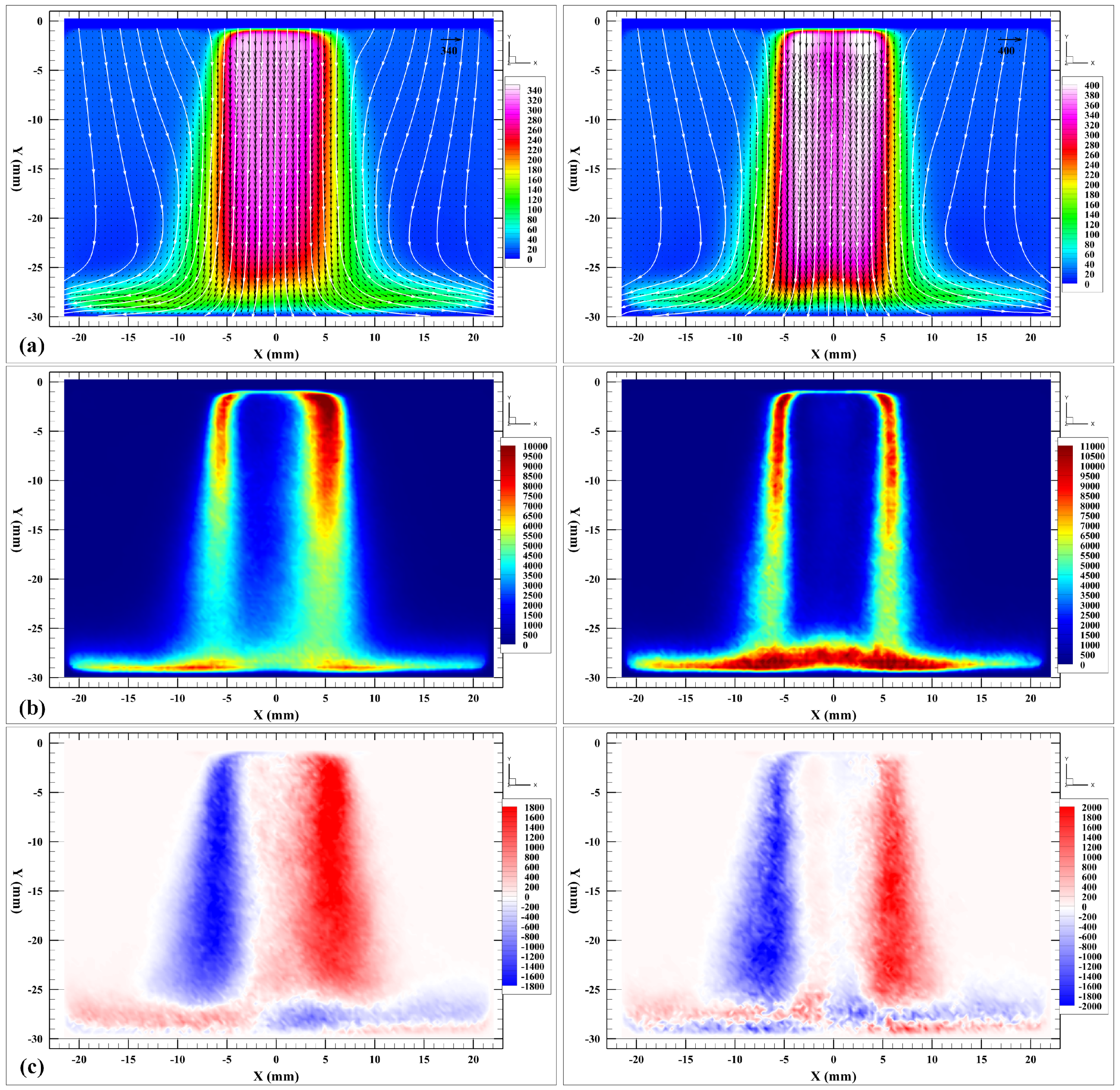
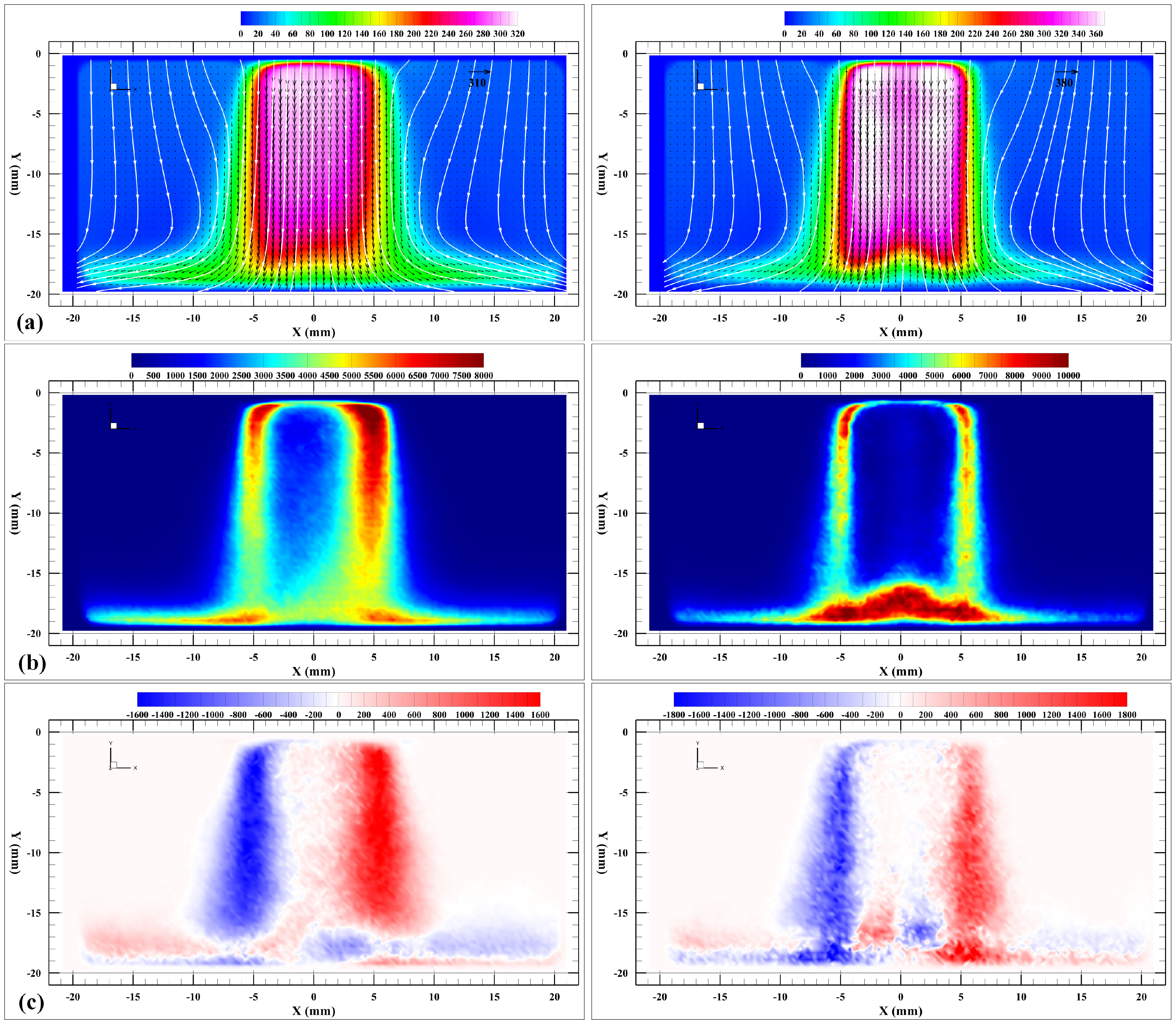
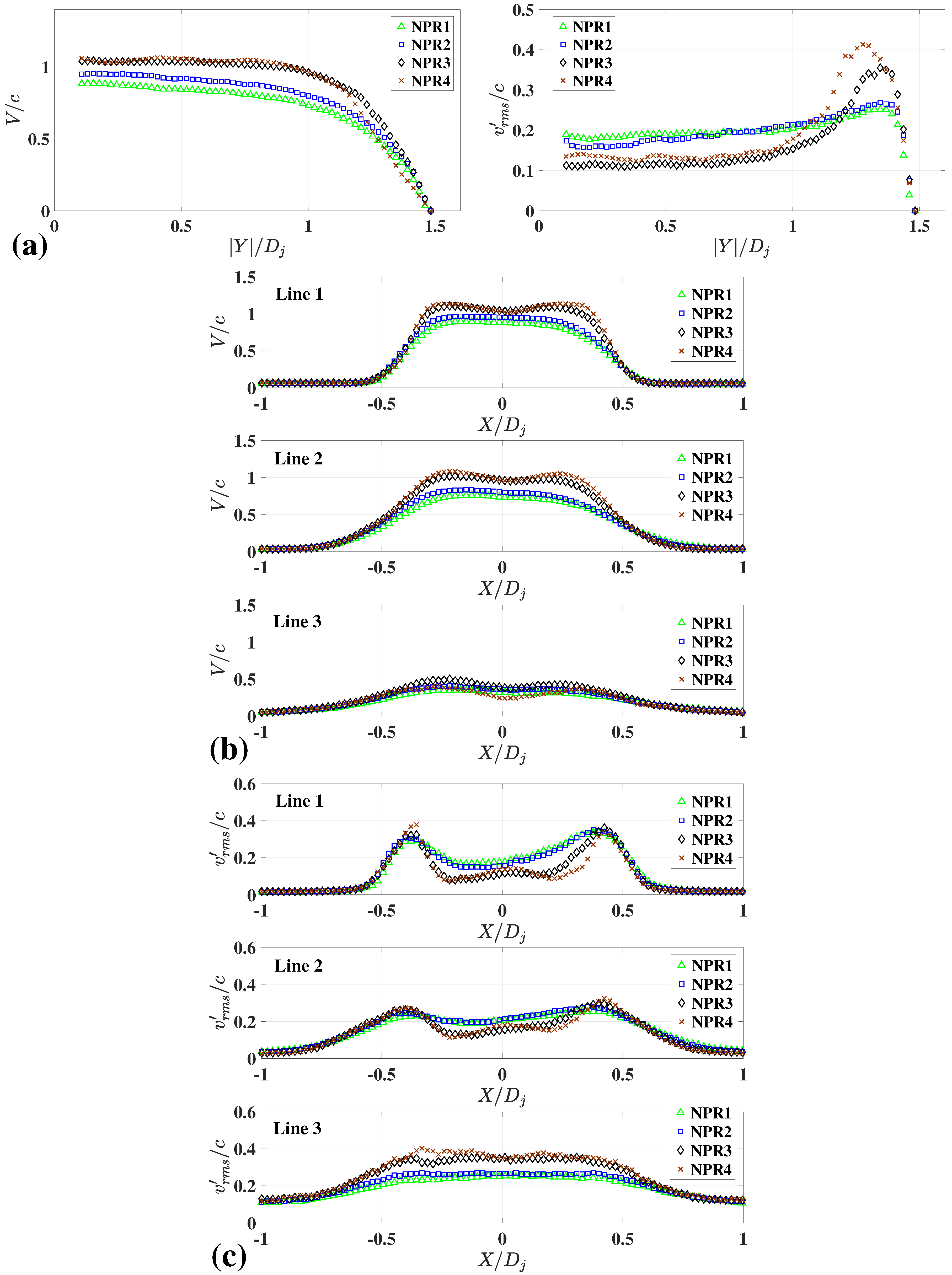
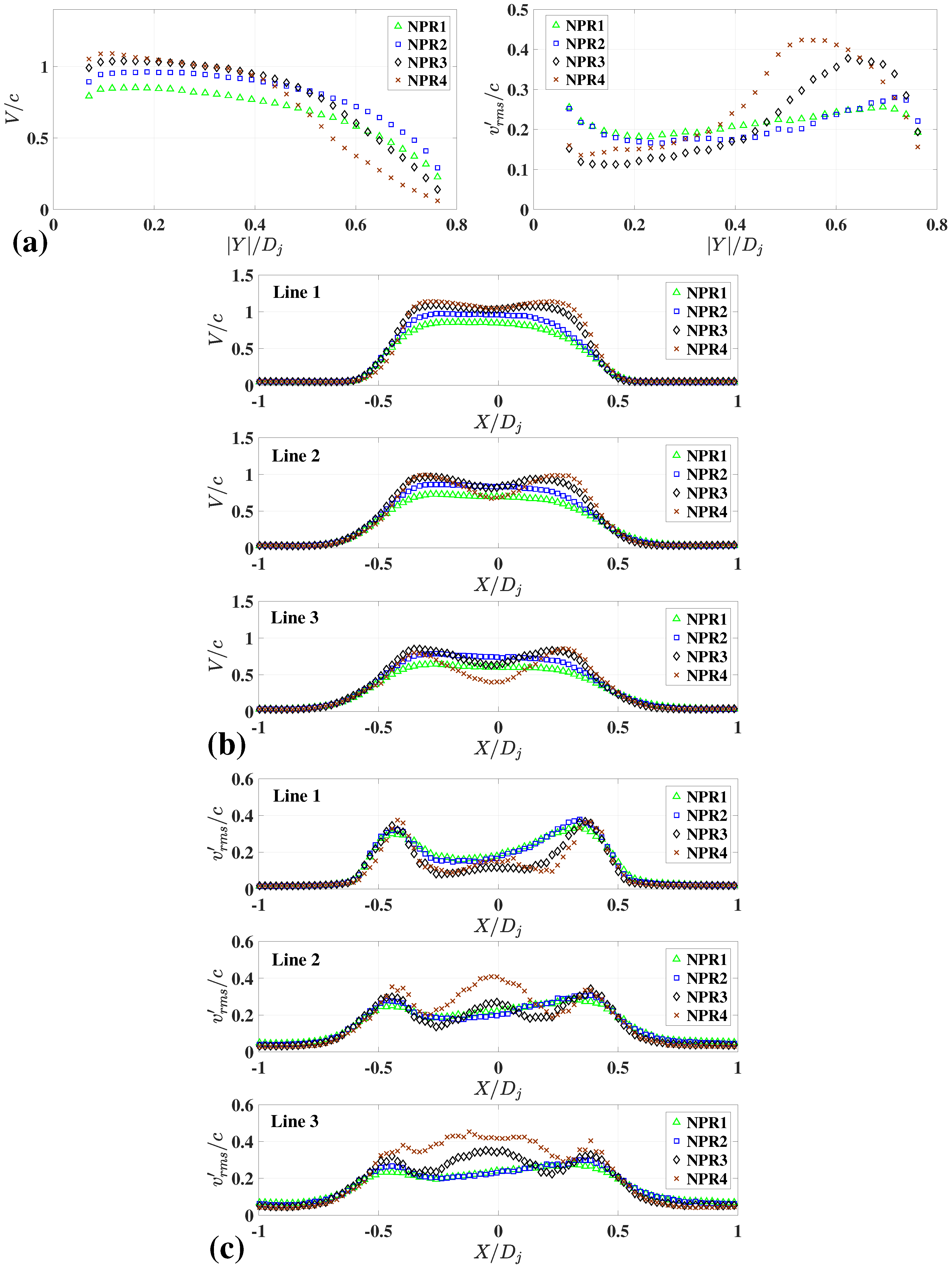
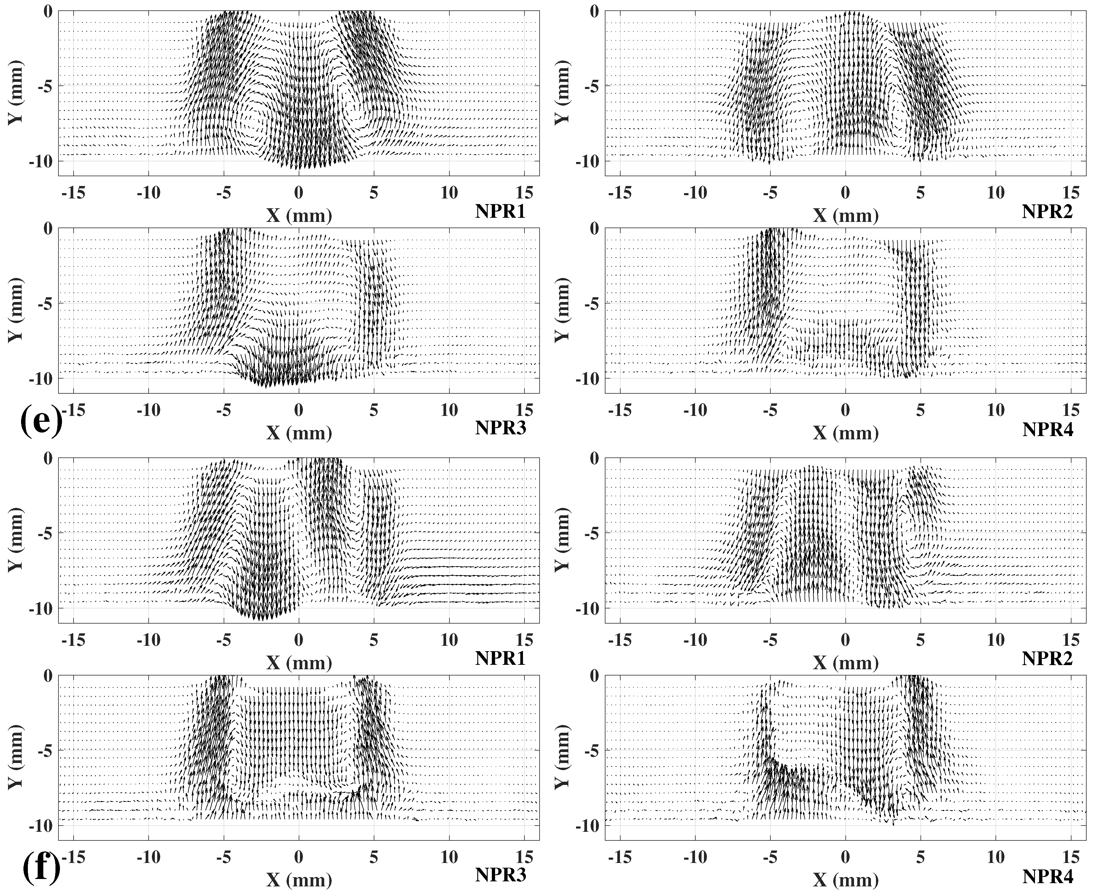
3.2. Experimental Results of Under-Expanded Impinging Jets for Various Nozzle-to-Plate Gaps and NPRs

In this section, we present the statistical results obtained from the 2D2C PIV measurements of under-expanded impinging jets for various nozzle-to-plate gaps e = 30 mm, 20, and 10 mm, and various values of NPRs, i.e., N P R 1 = 2 , N P R 2 = 2.2 , N P R 3 = 2.5 , and N P R 4 = 2.77 . Figure 4, Figure 5 and Figure 6 show the color contours of mean velocity fields, turbulent kinetic energy, and Reynolds stress for e = 30 mm, 20 mm, and 10 mm, respectively. In addition, for each specific spatial gap e, comparisons of the first- and second-order statistical profiles computed from the PIV measurements for various NPRs are presented in Figure 7, Figure 8 and Figure 9. Detailed discussions on the obtained results are followed.
As discussed in many previous studies, for examples those of Henderson [9], Sinibaldi et al. [18], Snedeker et al. [41], Donaldson et al. [42], Alvi and Iyer [43], and Wilke and Sesterhenn [7], the configuration of a turbulent jet impinging on a surface has a complex flow field, which can be roughly described as three regions. These include an upstream region, where the flow has behaviors like a free jet; an impingement region, where the flow structure is affected by the presence of the impingement plane; and a wall jet region, where the flow develops in the radial direction along the impingement surface. The flow field characteristics of these three regions depend on the values of NPRs and nozzle-to-plate distance e (Sinibaldi et al. [18]).
Figure 4(left), Figure 5(left) and Figure 6 illustrate the statistical results of under-expanded impinging jets with the nozzle-to-plate distances e = 30 mm, 20 mm, and 10 mm, respectively, that were obtained from velocity measurements at a low-pressure ratio N P R 2 = 2.2 . It is seen that the mean velocity fields at N P R 2 = 2.2 depict the potential core of the jet, and the deceleration of the jet flow in the axial direction due to the presence of the impingement plane. Besides, the impinging surface caused a deflection of the jet flow in the radial direction, which was immediately accelerated after the stagnation location. The radial wall jets were then formed and the wall boundary regions were established downstream from the impingement along the lateral direction. Due to a sudden expansion in the lateral direction at the nozzle outlet, shear layers were created from the nozzle edge and traveled further downstream until they impinged on the perpendicular surface. Color contours of the turbulent kinetic energy have shown dominant levels along the jet shear layers near the nozzle exit and on top of the surface where the shear layers impinged to the plane. The slight asymmetric feature seen in the k contours could be caused by the minor geometrical distortions of the nozzle outlet. It is noted that the test nozzle, which was removed from a practical system, had few minor distortions due to mechanical stresses from the installation, maintenance and operating conditions. Inside the shear layers, the maximal turbulence level reached almost 12 % of the mean jet velocity U j at the streamwise location y 1 = 1.5 (mm) near the nozzle exit. The turbulence levels reduced gradually until the shear layers reached the surface, and peaked again when the flow decelerated and developed as the wall jets. The negative and positive peaks in color contours of Reynolds stress u v appeared along the shear layers and their signs indicated the rotational signs of a contour-vortex pair formed downstream of the nozzle outlet.
Figure 4(right), Figure 5(right) and Figure 6 illustrate the statistical results of under-expanded impinging jets with the nozzle-to-plate distances e = 30 mm, 20 mm, and 10 mm, respectively, that were obtained from velocity measurements at a high-pressure ratio N P R 4 = 2.77 . It is noticeable that the color contours of velocity magnitude revealed the presence of a stand-off shock (normal shock) accompanied with a stagnation bubble in the impingement region. As the nozzle-to-plate distance decreased, the jet potential core ended in the region of flow deflection, where the axial and radial velocity components significantly decreased and increased, respectively. This region is also called stagnation flow region. In addition, color contours of turbulent kinetic energy clearly depict the peak values in the region of the stand-off shocks rather than in the shear layers as previously shown for the low-pressure ratio measurements. Such observation suggests that the turbulence fields can be also used as the indicator for the location of the stand-off shock (Cabrita et al. [4]). Krothapalli et al. [3] performed experimental studies of flow field and noise characteristics of an axisymmetric supersonic jet issuing from a sonic and a Mach 1.5 converging-diverging nozzle and impinging on a ground plane. These authors found that the stand-off shock was not always present in their experimental conditions with e / D j < 8 . In fact, Krothapalli et al. [3] discussed that the size, shape and presence of stand-off shock strongly depended on the values of NPRs and e / D j . Their experimental results of flow and acoustic characteristics have shown that the appearance and disappearance of the stand-off shock and the stagnation region could importantly contribute to the local aerodynamics and acoustic fields created by the sonic and supersonic impinging jets. In the experimental investigation by means of acoustic, velocity and wall pressure measurements of under-expanded impinging jets for NPRs from 2 to 3 and e / D j = 2 , 3, and 4, Sinibaldi et al. [18] described that behind the stand-off shock wave, there were a subsonic region and a supersonic region, and those were separated by a sonic line. In case that the pressure in the impingement region is small enough and the jet flow cannot overcome the maximum pressure, the jet flow is deflected and impinged at a certain distance from the surface to the stagnation region, which is formed by the outwards radial flow separating from the solid surface. In the mean flow field and turbulent kinetic energy obtained from PIV measurements in this study, it can be observed that the axial extension of the stand-off shock from the impingement surface increased when the nozzle-to-plate distance decreased.
Statistical profiles obtained from PIV measurements of under-expanded impinging jets various nozzle-to-plate distances e = 30 mm, 20 mm, and 10 mm, are compared in Figure 7, Figure 8 and Figure 9, respectively. The statistical results were computed from velocity vector fields corresponding to different values of NPRs, i.e., N P R 1 = 2 , N P R 2 = 2.2 , N P R 3 = 2.5 , and N P R 4 = 2.77 , and interpolated along the jet centerline and three radial lines.
Figure 7a, Figure 8a and Figure 9a show the centerline axial velocity variation with downstream distance for various configurations of impinging jets. For the impinging jets at N P R 4 = 2.77 , the mean centerline velocities remained nominally constant up to | Y | / D j = 1.82 , 0.93 , and 0.32 for e = 30 mm, 20 mm, and 10 mm, respectively. Further downstream, the axial velocity gradually reduced, which indicated the deceleration of the flow approaching the impingement plate. The presence of the stand-off shock in vicinity of the impingement surface is shown by the appearances of maximum peaks in profiles of v r m s / c . It can also be seen that for e = 30 mm, axial locations of v r m s / c peaks obtained for all values of NPRs are almost identical. However, when the nozzle-to-plate distance reduced to e = 20 mm and 10 mm, the axial locations of v r m s / c peaks were found to move further away from the solid surface at higher values of NPRs. For instance, peaks of v r m s / c were found at | Y | / D j = 0.72 , 0.62 , and 0.53 for PIV measurements of e = 10 mm with N P R 1 , N P R 3 , and N P R 4 , respectively.
In comparisons of normalized mean axial velocity, V / c , and normalized RMS fluctuating axial velocity, v r m s / c , along radial lines, it can be seen that these statistical profiles along Line 1 ( y = 2.54 ) mm did not reveal significant difference compared to those obtained from velocity measurements of free jets. This indicates that the flow structure near the nozzle outlet was not strongly influenced by the presence of the impingement surface. Further downstream of the nozzle outlet, the comparisons of statistical profiles showed an increase in RMS fluctuating velocity, and particularly the presence of local peaks at the jet centerline. An explanation for such observation could be the oscillation of the stand-off shock appeared on the solid surface (Sinibaldi et al. [18]).

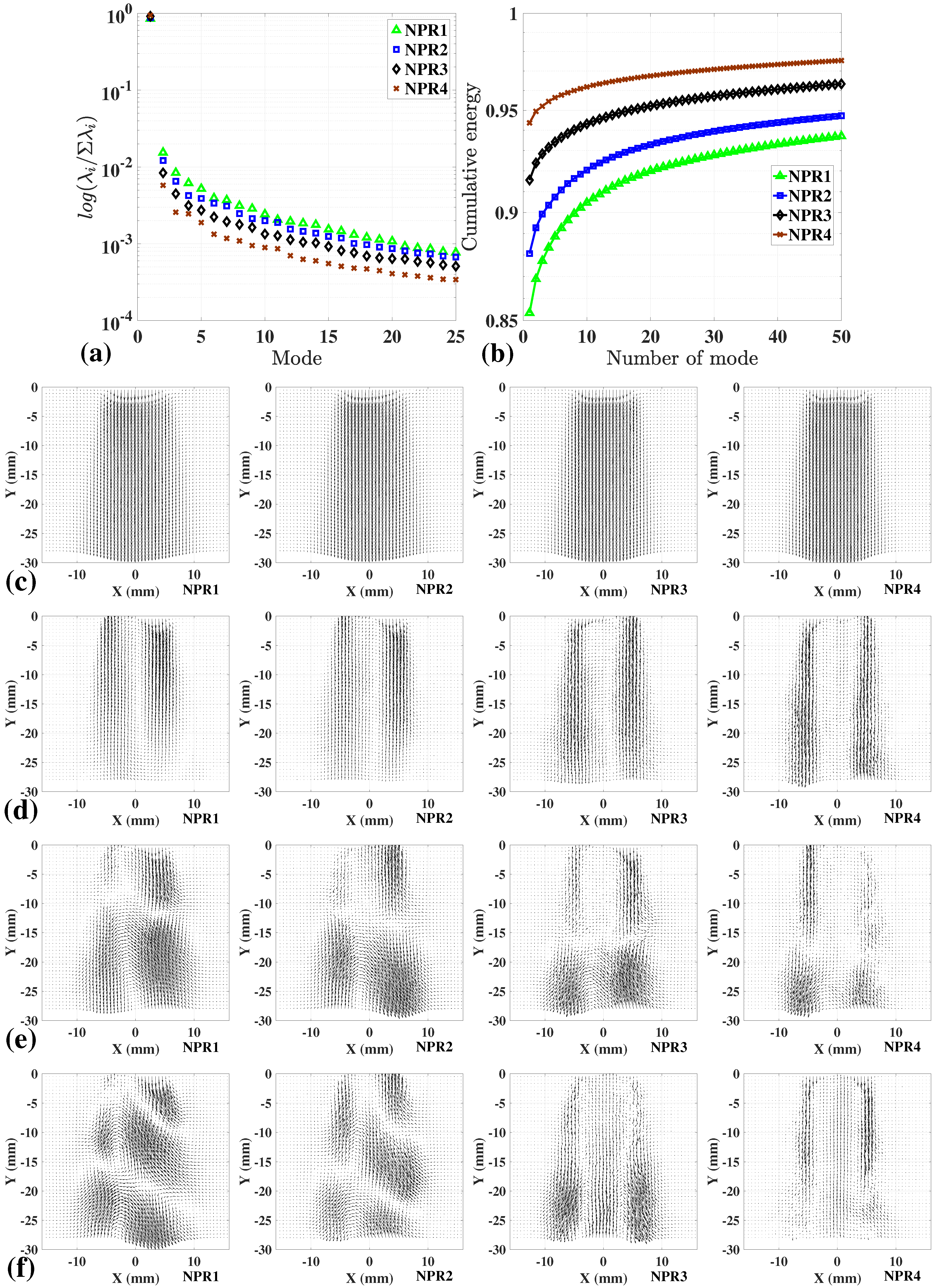
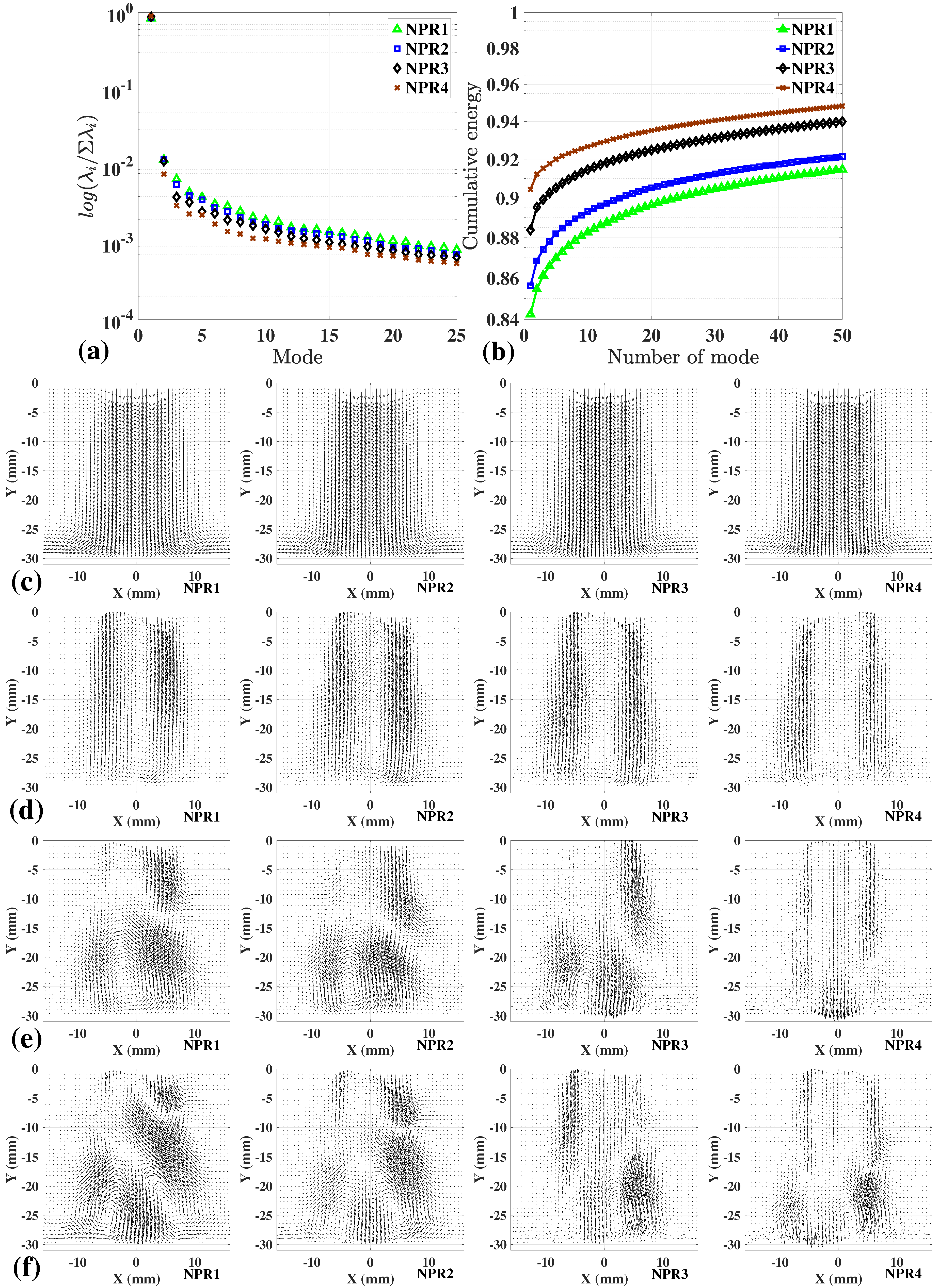
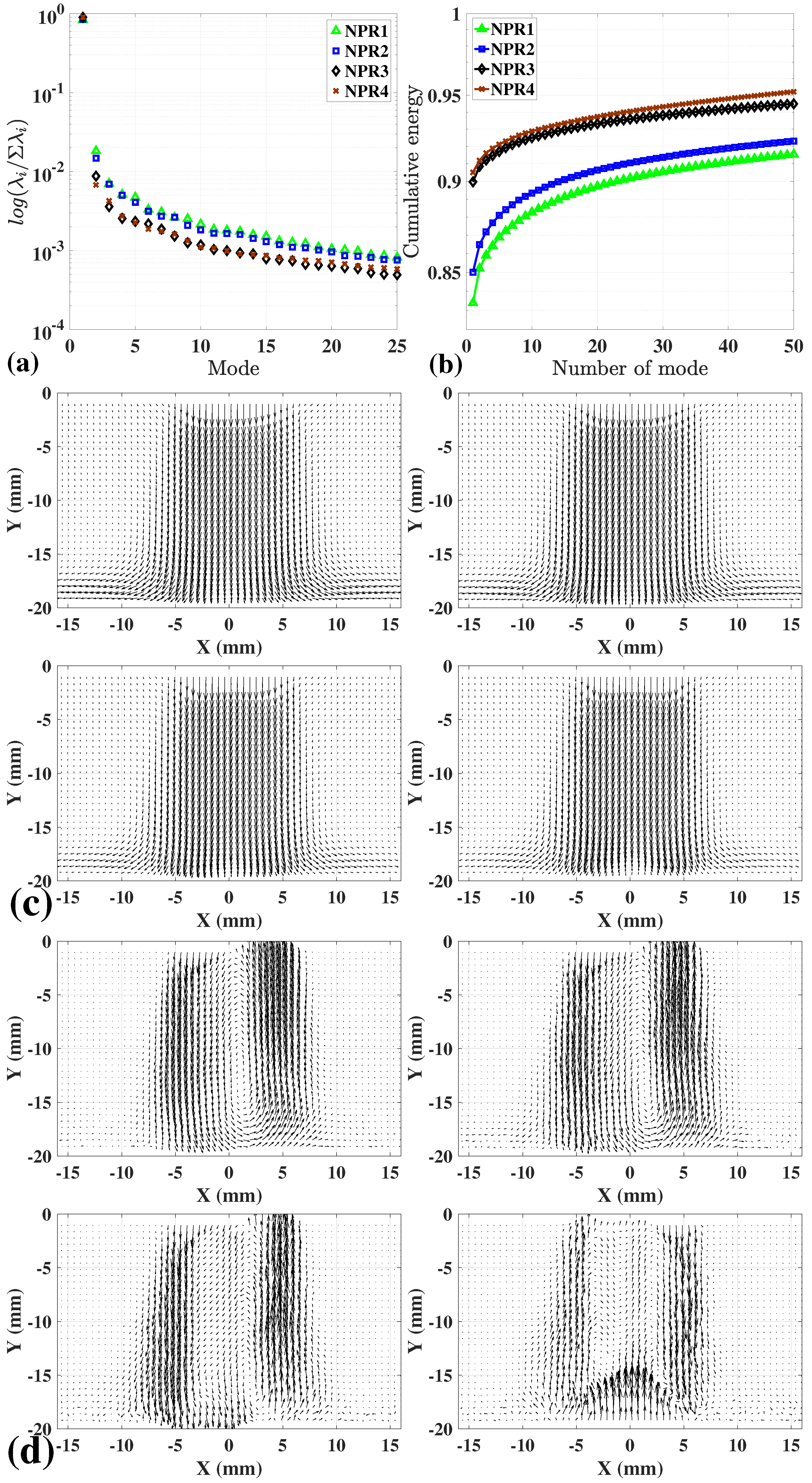
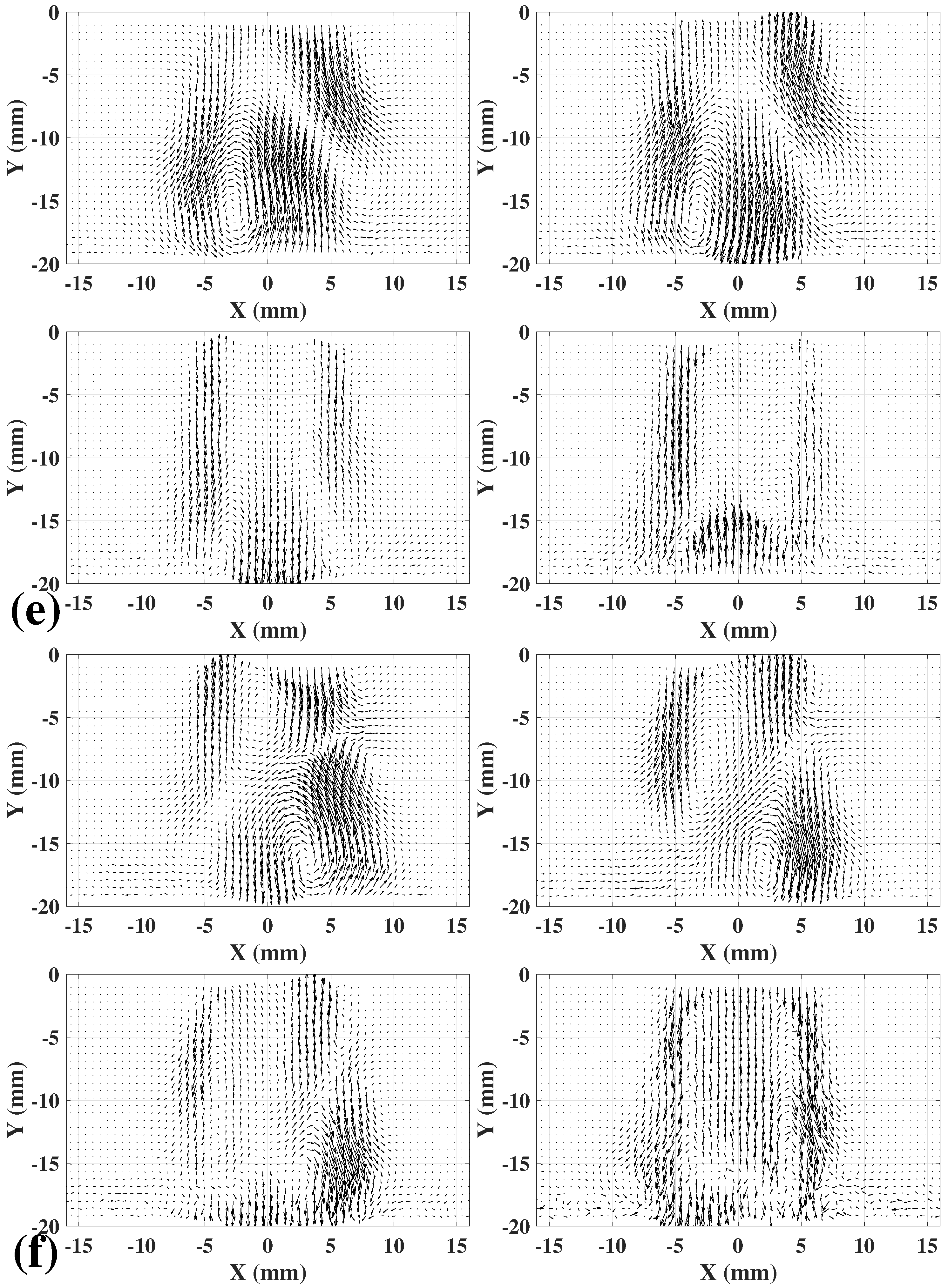
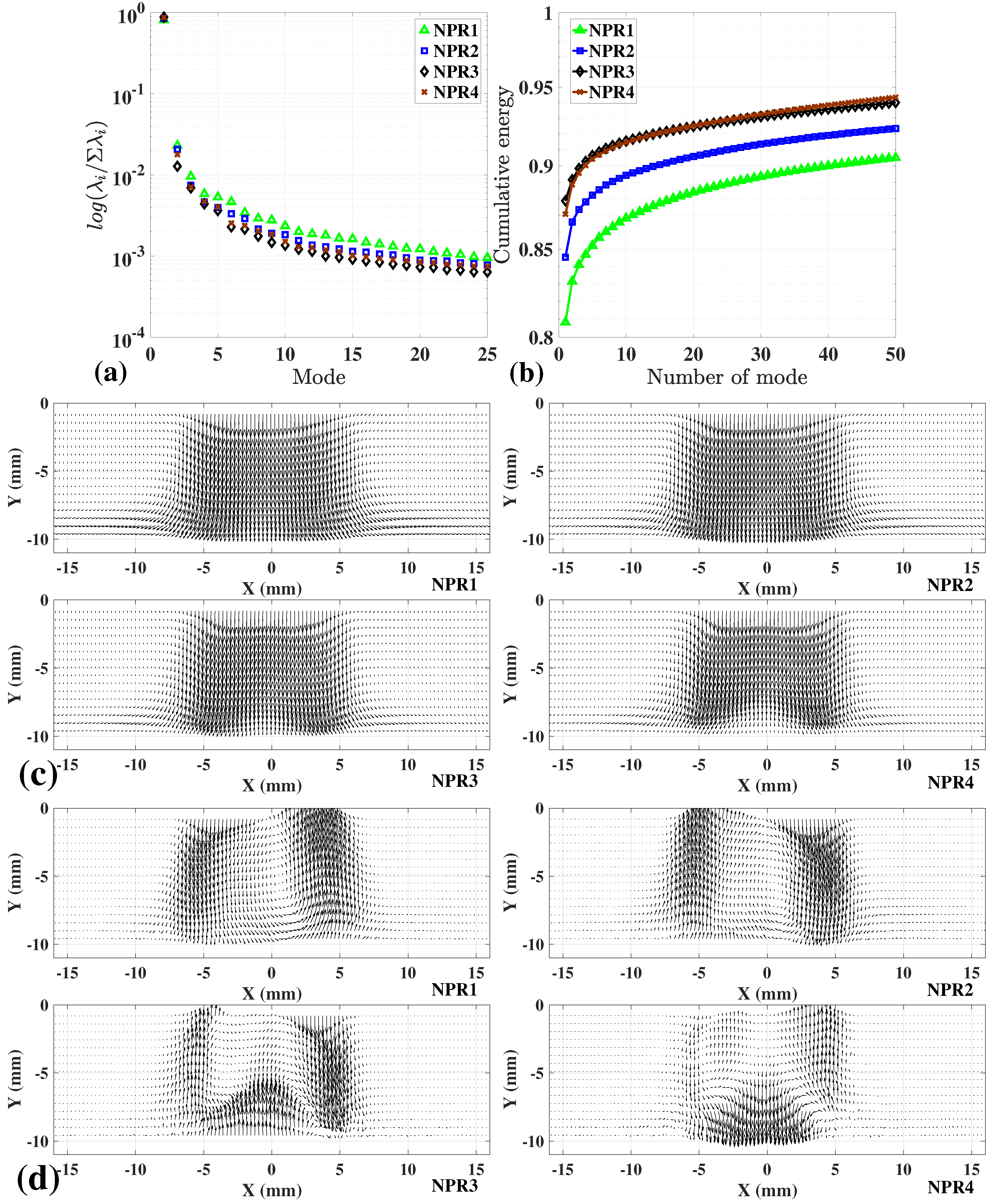
4. Proper Orthogonal Decomposition Analysis to the Free Jet and Impinging Jet Flows

This section describes the proper orthogonal decomposition (POD) analysis of the 2D2C PIV velocity snapshots using to extract the dominant flow structures that play important roles in the flow dynamics and acoustic characteristics of under-expanded free jets and impinging jets. The velocity vector fields were obtained from the flow measurements of free jets and impinging jets for various values of NPRs and nozzle-to-plate distances.
Lumley [44] introduced POD, i.e., also called or Karhunen-Loéve decomposition, into turbulence flow studies to identify statistically dominant flow features (coherent structures) in acquired experimental data and numerical simulations. For a given flow, the velocity field u ( x ) is decomposed into a set of spatially orthogonal modes and a set of temporal coefficients, which vary, respectively, only in space and time (Nguyen et al. [45]). The POD modes extracted from the velocity vector fields yield an optimal representation of the flow field such that, for any given number of modes, the two-norm of the truncation error between the original velocity data and the projection of the original velocity data onto such modes is minimized (Berkooz et al. [46], Holmes et al. [47]). In addition, the original velocity fields can be approximated or reconstructed using the few lowest-order POD modes that capture the highest amount of flow kinetic energy and the associated temporal coefficients (Nguyen et al. [48]). Detailed descriptions of the POD analysis can be reviewed in Berkooz et al. [46], Holmes et al. [47], and Sirovich and Kirby [49]. A brief review of the snapshot POD of the velocity fields is provided here. A POD analysis of a given velocity vector field u ( x , 0 t T ) (T is a finite time direction) can be described as
u ( x , t ) k = 1 N ζ k ( t ) ψ ( x ) ,
where N is the number of velocity snapshots, ζ k ( t ) and ψ ( x ) are the POD temporal coefficients and POD basis functions, respectively. ψ ( x ) are the eigenfunctions of a two-point correlation matrix R ( x , x ) defined as
R ( x , x ) = 1 T 0 T u ( x , t ) · u ( x , t ) d t .
It is common that velocity vector fields obtained by experiments and numerical simulations are discrete, the snapshot POD (Sirovich and Kirby [49]) is usually used. In the current study, we apply the snapshot POD analysis to the collections of 2D2C PIV velocity vector fields obtained from PIV measurements of free jets and impinging jets corresponding to various values of nozzle-to-plate distances e and NPRs. First, a correlation matrix is defined as
C i j = 1 N u ( x , t i ) · u ( x , t j ) d x ,
and the POD temporal coefficients and POD basis functions are computed as
Ψ k ( x ) = i = 1 N α k i u ( x , t i ) ζ k ( t j ) = N i = 1 N α k i C i t j .
In the above equations, coefficients α k i are defined as
α k i = υ i k N m = 1 N r = 1 N υ m k υ r k C m r ,
where υ i k is the ith element of the eigenvector υ k associated to the eigenvalue λ k of the matrix C . The correlation matrix C is built from instantaneous velocity snapshots, therefore, a derived eigenvalue λ k associated with a POD mode k represents the flow kinetic energy contained by that mode.
In our POD calculation, the eigenvalue λ associated with each POD mode is proportional to the kinetic energy contained in that mode. The decomposition yields statistically dominant flow structures in the few lowest-order POD modes. These modes capture most of the flow’s kinetic energy and are typically associated with large-scale structures. Besides, the POD basis functions computed from these velocity snapshots yield an optimal representation of the flow field in the sense that, for any given number of basis functions, the Hilbert norm of the truncation error between the original velocity data and the projection of the original velocity data onto these basis functions is minimized. The present PIV setup allows us to capture several hundred instantaneous velocity fields. A set of few hundreds PIV realizations suffice for a POD analysis to reveal the statistically dominant structures of the flow (Nguyen et al. [24]).
Figure 10, Figure 11, Figure 12 and Figure 13 illustrate results from the POD analysis of velocity fields obtained from 2D2C PIV measurements of free jets and impinging jets for various nozzle-to-plate distances of e = 30 mm, 20 mm, and 10 mm, respectively. The results are also presented for various values of NPRs. Figure 10a,b, Figure 11a,b, Figure 12a,b and Figure 13a,b show the energy spectra and the cumulative kinetic energy computed from the POD analysis of PIV instantaneous velocity vector fields for N P R 1 , N P R 2 , N P R 3 , and N P R 4 . In addition, the kinetic energy fractions contained in low-order POD modes 1–4, i.e., Ψ 1 Ψ 4 , are listed in Table 2 for different nozzle-to-plate distances e and for values of N P R 1 , N P R 2 , N P R 3 , and N P R 4 .
In all the POD analysis to the PIV velocity fields of under-expanded free jets and impinging jets, the kinetic energy fractions contained in the first POD modes were found to increase when the NPRs increased. It is noted that the first POD modes are considered approximately equivalent to the time-averaged velocity fields and such observations can be confirmed in the representation of POD Mode 1 displayed in Figure 10c, Figure 11c, Figure 12c and Figure 13c. For instance, in the POD analysis of impinging jets with e = 30 mm ( e / D j = 2.46 ), the kinetic energy in the first POD modes increased from 84.5 % to 90.4 % when NPRs increased from 2 to 2.77 . In comparisons among the first POD modes of the velocity decomposition for the free jets and impinging jets with different spatial gaps e, it is seen that for the same values of NPRs, POD Mode 1 of the under-expanded free jets had the highest energy fractions. Besides, it is found that the POD Mode 1 captured lower levels of the flow kinetic energy when the spatial gaps e reduced from 30 mm to 10 mm. For all the POD velocity decompositions of under-expanded free jets and impinging jets, the kinetic energy levels of the low-order POD modes 2, 3, and 4 were less than 3 % . This observation indicates that the flow fields of the free jets and impinging jets in this study are highly turbulent and the flow kinetic energy is widely distributed over many flow-structures whose scales are smaller than the time-averaged flows.
For the under-expanded free jets, the total flow kinetic energy levels contained in the first 100 low-order POD modes varied between 96.4 % and 98.3 % when NPRs increased from N P R 1 = 2 to N P R 4 = 2.77 . Analogously, for the under-expanded impinging jets, these values ranged from 94.5 % to 96.1 % with e = 30 mm, from 95.4 % to 96.7 % with e = 20 mm, and from 94.6 % to 96.17 % with e = 10 mm when N P R s increased from 2 to 2.77 , respectively. Sirovich and Kirby [49] suggested a 99 % of total flow energy as a cutoff to accurately represent the flowfield, while Palacios et al. [50] discussed that a 75 % of total flow energy could be sufficient for a reasonable representation of the system. Moreno et al. [51] applied POD analysis to PIV velocity vectors obtained from experimental measurements of supersonic rectangular convergence-divergence jet at a Mach number of 1.44 . The authors quantified the accuracy of low-order flow reconstruction using the first two POD modes capturing 90 % of the total flow energy. They reported the mean square error of less than 1.2 % , thus concluded that the reconstructed flowfield using two modes is a good representation of the flowfield (Moreno et al. [51]). In the current study, it is found that for the under-expanded free jets, the total flow kinetic energy captured by the first two POD modes are 87.15 % , 89.92 % , 92.6 % , and 94.95 % corresponding to N P R 1 = 2 , N P R 2 = 2.2 , N P R 3 = 2.5 , and N P R 4 = 2.77 , respectively. These values are comparable to those reported in the study of Moreno et al. [51].
Figure 10c–f, Figure 11c–f, Figure 12c–f and Figure 13c–f show the in-plane components of the low-order POD modes 1, 2, 3, and 4 extracted from the POD velocity decomposition for the under-expanded free jets and impinging jets with e = 30 mm, 20 mm, and 10 mm, respectively. In these figures, results from the POD analysis of velocity fields for various N P R s are also illustrated for comparisons. It is noted that in the current POD velocity decomposition, the POD spatial functions, i.e., POD modes, were non-dimensional.
It is obviously seen that the first POD modes displayed flow structures that are statistically similar to the time-averaged velocity fields for all the studied cases. For the specific values of the spatial gap e and NPR, lower-order POD modes illustrated the statistically dominant flow structures with larger shapes and sizes compared with those structures depicted by the higher-order POD modes. In addition, for a specific value of e, while the spatial flow structures illustrated by POD mode 1 are similar when NPRs increased, the dominant flow structures revealed by POD modes 2, 3, and 4 were not entirely analogous. One may also find that for results from the POD analysis to velocity fields of N P R 1 = 2 and N P R 2 = 2.2 , the extracted dominant flow structures are the same, while those extracted from the POD analysis to velocity fields of N P R 3 = 2.5 and N P R 4 = 2.77 are quite similar. This indicates the differences in large-scale flow structures and transition of energy-contained eddies when the under-expanded free jet and impinging jet flows have undergone from near sonic to supersonic conditions.
It is noticed that the presence of stand-off shock is captured in the visualization of POD mode 2, especially for the value of N P R 4 = 2.77 . Additionally, one may find that the POD modes 2, 3, and 4 obtained for lower N P R values displayed the large-scale flow structures with considerable large shapes and sizes compared to the nozzle diameter D j and spatial gaps e. Furthermore, spatial locations of these structures are found to distribute within the jet core and the inner sides of the shear layers. On the other hand, for higher values of NPRs, the statistically dominant flow structures depicted by the low-order POD modes 2, 3, and 4 were likely the resemblances of stand-off shock near the impingement surface and the jet shear layers. Such observations confirmed the discussions on the characteristics of flow fields and acoustics of the supersonic impinging jets in many of previous studies, for examples studies of Krothapalli et al. [3], Tam and Ahuja [14], Henderson and Powell [15], Henderson [16], Sinibaldi et al. [18], Ho and Nosseir [20], Nosseir and Ho [21], Wilke and Sesterhenn [52], and Wilke and Sesterhenn [7], to name a few. In their experimental and numerical investigations, these authors studied and described the mechanism of acoustic generation as a feedback loop in supersonic flows. For instance, Tam and Ahuja [14] and Henderson and Powell [15] discussed that the instability waves appeared in the jet shear layers supplied the energy for the feedback loop. Generated by acoustic excitation in the vicinity of the nozzle outlet, these waves propagate further downstream and grow in size as the large-scale flow structures that are captured in flow visualizations of Krothapalli et al. [3], and in our experimental velocity vector fields. Moreover, Krothapalli et al. [3], Henderson [16] and Sinibaldi et al. [18] suggested that when these large-scale vortical structures impinging on the solid wall, they generate coherent pressure fluctuations, yielding acoustic waves at significant strengths. Later, the resulted acoustic waves travel in the upstream direction and eventually reach the nozzle outlet. Such interactions excite the jet shear layers and cause the generation of instability waves, thus close the feedback loop (Krothapalli et al. [3]). Using direct numerical simulations of subsonic and supersonic impinging jets, Wilke and Sesterhenn [52] and Wilke and Sesterhenn [7] have intensively shown that primary vortices are generated in the jet shear layers and initially transported with the flows. The impact of the jet shear layers to the solid surface generates new vortices (secondary vortices) that pair with the primary ones. Wilke and Sesterhenn [53] also discussed that the formation of primary and secondary vortices is a periodical phenomenon associated with a characteristic frequency. The flow mode can be distorted due to interactions between large-scale flow structures in the jet and shear layers, and the feedback waves resulted from the impingement.
Although the current 2D2C PIV measurements were not able to provide the temporal evolution of the large-scale structures, their existences can be confirmed in Figure 10, Figure 11, Figure 12 and Figure 13 as the results of velocity decomposition via POD analysis. The results from the POD velocity decomposition have revealed the appearances of statistically large-scale flow structures in the regions of stand-off shock, i.e., in the vicinity of impingement surface, and in the regions of jet shear layers. It is found that the first POD modes representing the mean flow fields of the free jets captured higher kinetic energy levels than those of the jet impinging on the solid surface. However, the flow kinetic energy levels contained in the low-order POD modes, presenting the coherent large-scale structures, increased when the nozzle-to-plate distances decreased. The statistically dominant large-scale structures with considerable sizes and shapes are found within regions between the jet core and shear layers for lower NPRs. However, for higher NPRs, the large-scale structures are resemblances of the stand-off shock near the solid surface and the jet shear layers.
It is noted that in this study, the velocity snapshots were obtained from PIV measurements with a sampling rate of 15 Hz, facilitating the POD analysis to the statistically independent snapshots to form the POD spatial basis functions. The current experimental setup, however, is not able to provide transient behavior of the flowfield and acoustic characteristics of under-expanded supersonic free jets and impinging jets. Even at moderate supersonic speeds, it is still a challenge for current time-resolved PIV systems to obtain large enough numbers of velocity snapshots that could enable low-dimensional analysis (Berry et al. [54]). An experimental setup combining a PIV system for velocity measurement and microphone system for acoustic measurement could provide details about the flowfield and noise characteristics of supersonic free jets and impinging jets. Experimental measurements of flowfield and acoustics as can be reviewed in numerous studies of Krothapalli et al. [3], Henderson [16], Henderson et al. [17], Sinibaldi et al. [18], Alvi and Iyer [43], and Guariglia et al. [55], to name a few. With the recent improvement in digital imaging cameras, high-speed schlieren is enable to acquire large datasets of time-resolved flowfield information (Berry et al. [56]), although the measured quantities are scalars derived from density gradients (Berry et al. [54]). The statistical dominant flow structures and dynamical evolution of large-scale flow structures can be extracted from the time-resolved schlieren images or from the time-resolved velocity fields obtained from large-eddy simulations using POD (Weightman et al. [10], Berry et al. [54], Nair et al. [57], Berry et al. [58], Weightman et al. [59]), spectral POD (Karami and Soria [60]), and dynamic mode decomposition (DMD) (Berry et al. [56]) techniques.

5. Conclusions

In this paper, we obtained 2D2C PIV measurements of free jets and impinging jets with various nozzle pressure ratios (NPRs) ranging from 2 to 2.77 . The velocity profiles, RMS fluctuating velocity, and Reynolds stress distributions were obtained for different values of nozzle-to-plate distances e = 10 mm, 20 mm, and 30 mm. The mean axial velocity profiles obtained at low NPRs had maximum values along the jet centerline, while those at high NPRs showed the maximum velocity along the nozzle perimeter. Profiles of RMS fluctuating axial velocity for N P R 1 and N P R 2 had two local peaks on both sides of the jet shear layers, while profiles of v r m s for N P R 3 and N P R 4 had an additional peak at X / D j = 0 . Results obtained from the PIV measurements of impinging jets have shown the jet flow deflection caused by the impinging surface. The jet shear layers were created from the nozzle outlet and traveled further downstream until they impinged on the solid surface. The turbulent kinetic energy contours illustrated significant high levels along the shear layers near the nozzle exit and on top of the solid surface, where the jet shear layers impinged. At the high NPRs, the presence of a stand-off shock and a stagnation region was observed in the color contours of velocity magnitude, and the peaks of turbulent kinetic energy was found in the region of stand-off shock. In comparisons of statistical profiles obtained from PIV measurements of impinging jets for various values of spatial gaps and NPRs, the presence of stand-off shock was shown by the appearances of maximum peaks of v r m s profiles in the vicinity of impingement surface. Such phenomena were caused by the oscillation of stand-off shock appeared on the solid surface. In addition, it is found that the axial locations of v r m s peaks moved further away from the impingement surface at higher values of NPRs.
Finally, we applied the POD analysis to the velocity snapshots obtained from PIV measurements of free jets and impinging jets for various values to nozzle-to-plate distances e and nozzle pressure ratios (NPRs) to reveal the most dominant flow structures that play important roles in the flow dynamics and acoustic characteristics of subsonic and supersonic jets. The POD velocity decompositions have shown that the coherent large-scale structures extracted from the velocity fields of N P R 1 = 2 and N P R 2 = 2.2 were different when compared to those extracted from the velocity fields of N P R 3 = 2.5 and N P R 4 = 2.77 . This indicated the differences in large-scale flow structures and transition of energy-contained eddies when the impinging jet flows have undergone from subsonic to supersonic conditions. For high values of NPRs, the presence of stand-off shock was revealed in the visualization of low-order POD modes, while the large-scale structures were found to distribute within regions between the jet core and shear layers for lower NPRs.

Author Contributions

B.M. performed the conceptualization design, the experimental design as well as the flow visualization measurements. D.T.N. supervised the project, performed the flow analysis and the modal decomposition, and wrote the manuscript. Y.H. supervised and validated the project as well as contributed to the final editing and review of the manuscript.

Funding

This research received no external funding.

Acknowledgments

The authors gratefully acknowledge Courtney Powell, Camila Freitas Matozinhos and Gabriel Caio Queiroz Tomaz, who are graduate students at Texas A&M University, for their support with the flow measurements.

Conflicts of Interest

The authors declare no conflict of interest.

References

  1. Saddington, A.J.; Lawson, N.; Knowles, K. An experimental and numerical investigation of under-expanded turbulent jets. Aeronaut. J. 2004, 108, 145–152. [Google Scholar] [CrossRef]
  2. Hadžiabdić, M.; Hanjalić, K. Vortical structures and heat transfer in a round impinging jet. J. Fluid Mech. 2008, 596, 221–260. [Google Scholar] [CrossRef]
  3. Krothapalli, A.; Rajkuperan, E.; Alvi, F.; Lourenco, L. Flow field and noise characteristics of a supersonic impinging jet. J. Fluid Mech. 1999, 392, 155–181. [Google Scholar] [CrossRef]
  4. Cabrita, P.; Saddington, A.; Knowles, K. PIV measurements in a twin-jet STOVL fountain flow. Aeronaut. J. 2005, 109, 439–449. [Google Scholar] [CrossRef]
  5. Saddington, A.; Knowles, K.; Cabrita, P. Flow measurements in a short takeoff, vertical landing fountain: Parallel jets. J. Aircr. 2008, 45, 1736–1743. [Google Scholar] [CrossRef]
  6. Saddington, A.; Knowles, K.; Cabrita, P. Flow Measurements in a Short Takeoff, Vertical Landing Fountain: Splayed Jets. J. Aircr. 2009, 46, 874–882. [Google Scholar] [CrossRef]
  7. Wilke, R.; Sesterhenn, J. Statistics of fully turbulent impinging jets. J. Fluid Mech. 2017, 825, 795–824. [Google Scholar] [CrossRef] [Green Version]
  8. Franquet, E.; Perrier, V.; Gibout, S.; Bruel, P. Free underexpanded jets in a quiescent medium: A review. Prog. Aerosp. Sci. 2015, 77, 25–53. [Google Scholar] [CrossRef]
  9. Henderson, L. Experiments on the impingement of a supersonic jet on a flat plate. Z. Angew. Math. Phys. ZAMP 1966, 17, 553–569. [Google Scholar] [CrossRef]
  10. Weightman, J.L.; Amili, O.; Honnery, D.; Soria, J.; Edgington-Mitchell, D. An explanation for the phase lag in supersonic jet impingement. J. Fluid Mech. 2017, 815. [Google Scholar] [CrossRef]
  11. Uzun, A.; Kumar, R.; Hussaini, M.Y.; Alvi, F.S. Simulation of tonal noise generation by supersonic impinging jets. AIAA J. 2013, 51, 1593–1611. [Google Scholar] [CrossRef]
  12. Akamine, M.; Okamoto, K.; Gee, K.L.; Neilsen, T.B.; Teramoto, S.; Okunuki, T.; Tsutsumi, S. Effect of Nozzle–Plate Distance on Acoustic Phenomena from Supersonic Impinging Jet. AIAA J. 2018, 56, 1943–1952. [Google Scholar] [CrossRef]
  13. Brown, G.L.; Roshko, A. On density effects and large structure in turbulent mixing layers. J. Fluid Mech. 1974, 64, 775–816. [Google Scholar] [CrossRef]
  14. Tam, C.K.; Ahuja, K. Theoretical model of discrete tone generation by impinging jets. J. Fluid Mech. 1990, 214, 67–87. [Google Scholar] [CrossRef]
  15. Henderson, B.; Powell, A. Experiments concerning tones produced by an axisymmetric choked jet impinging on flat plates. J. Sound Vib. 1993, 168, 307–326. [Google Scholar] [CrossRef]
  16. Henderson, B. The connection between sound production and jet structure of the supersonic impinging jet. J. Acoust. Soc. Am. 2002, 111, 735–747. [Google Scholar] [CrossRef] [PubMed]
  17. Henderson, B.; Bridges, J.; Wernet, M. An experimental study of the oscillatory flow structure of tone-producing supersonic impinging jets. J. Fluid Mech. 2005, 542, 115–137. [Google Scholar] [CrossRef]
  18. Sinibaldi, G.; Marino, L.; Romano, G.P. Sound source mechanisms in under-expanded impinging jets. Exp. Fluids 2015, 56, 105. [Google Scholar] [CrossRef]
  19. Gojon, R.; Bogey, C.; Marsden, O. Investigation of tone generation in ideally expanded supersonic planar impinging jets using large-eddy simulation. J. Fluid Mech. 2016, 808, 90–115. [Google Scholar] [CrossRef] [Green Version]
  20. Ho, C.M.; Nosseir, N.S. Dynamics of an impinging jet. Part 1. The feedback phenomenon. J. Fluid Mech. 1981, 105, 119–142. [Google Scholar] [CrossRef]
  21. Nosseir, N.S.; Ho, C.M. Dynamics of an impinging jet. Part 2. The noise generation. J. Fluid Mech. 1982, 116, 379–391. [Google Scholar] [CrossRef]
  22. Kays, W.M. Convective Heat and Mass Transfer; Tata McGraw-Hill Education: New York, NY, USA, 2012. [Google Scholar]
  23. Solovitz, S.A.; Mastin, L.G.; Saffaraval, F. Experimental study of near-field entrainment of moderately overpressured jets. J. Fluids Eng. 2011, 133, 051304. [Google Scholar] [CrossRef]
  24. Nguyen, T.; Pellé, J.; Harmand, S.; Poncet, S. PIV measurements of an air jet impinging on an open rotor-stator system. Exp. Fluids 2012, 53, 401–412. [Google Scholar] [CrossRef] [Green Version]
  25. Nguyen, T.D.; Souad, H. PIV measurements in a turbulent wall jet over a backward-facing step in a three-dimensional, non-confined channel. Flow Meas. Instrum. 2015, 42, 26–39. [Google Scholar] [CrossRef]
  26. Raffel, M.; Willert, C.E.; Wereley, S.; Kompenhans, J. Particle Image Velocimetry: A Practical Guide; Springer: Berlin, Germany, 2013. [Google Scholar]
  27. Scarano, F. Overview of PIV in supersonic flows. In Particle Image Velocimetry; Springer: Berlin, Germany, 2007; pp. 445–463. [Google Scholar]
  28. Alvi, F.; Ladd, J.; Bower, W. Experimental and computational investigation of supersonic impinging jets. AIAA J. 2002, 40, 599–609. [Google Scholar] [CrossRef]
  29. Mitchell, D.; Honnery, D.; Soria, J. Particle relaxation and its influence on the particle image velocimetry cross-correlation function. Exp. Fluids 2011, 51, 933. [Google Scholar] [CrossRef]
  30. Samimy, M.; Lele, S. Motion of particles with inertia in a compressible free shear layer. Phys. Fluids A Fluid Dyn. 1991, 3, 1915–1923. [Google Scholar] [CrossRef]
  31. Erdem, E.; Saravanan, S.; Lin, J.; Kontis, K. Experimental Investigation of Transverse Injection Flowfield at March 5 and the Influence of Impinging Shock Wave. In Proceedings of the 18th AIAA/3AF International Space Planes and Hypersonic Systems and Technologies Conference, Tours, France, 24–28 September 2012; p. 5800. [Google Scholar]
  32. Ragni, D.; Schrijer, F.; Van Oudheusden, B.; Scarano, F. Particle tracer response across shocks measured by PIV. Exp. Fluids 2011, 50, 53–64. [Google Scholar] [CrossRef]
  33. Eckstein, A.C.; Charonko, J.; Vlachos, P. Phase correlation processing for DPIV measurements. Exp. Fluids 2008, 45, 485–500. [Google Scholar] [CrossRef]
  34. Eckstein, A.; Vlachos, P.P. Digital particle image velocimetry (DPIV) robust phase correlation. Meas. Sci. Technol. 2009, 20, 055401. [Google Scholar] [CrossRef]
  35. Westerweel, J. Efficient detection of spurious vectors in particle image velocimetry data. Exp. Fluids 1994, 16, 236–247. [Google Scholar] [CrossRef]
  36. Timmins, B.H.; Wilson, B.W.; Smith, B.L.; Vlachos, P.P. A method for automatic estimation of instantaneous local uncertainty in particle image velocimetry measurements. Exp. Fluids 2012, 53, 1133–1147. [Google Scholar] [CrossRef]
  37. Wilson, B.M.; Smith, B.L. Uncertainty on PIV mean and fluctuating velocity due to bias and random errors. Meas. Sci. Technol. 2013, 24, 035302. [Google Scholar] [CrossRef]
  38. Charonko, J.J.; Vlachos, P.P. Estimation of uncertainty bounds for individual particle image velocimetry measurements from cross-correlation peak ratio. Meas. Sci. Technol. 2013, 24, 065301. [Google Scholar] [CrossRef]
  39. Boomsma, A.; Bhattacharya, S.; Troolin, D.; Pothos, S.; Vlachos, P. A comparative experimental evaluation of uncertainty estimation methods for two-component PIV. Meas. Sci. Technol. 2016, 27, 094006. [Google Scholar] [CrossRef]
  40. Saffaraval, F.; Solovitz, S.A. Near-exit flow physics of a moderately overpressured jet. Phys. Fluids 2012, 24, 086101. [Google Scholar] [CrossRef]
  41. Snedeker, R.S.; Donaldson, C.D. A study of free jet impingement. Part 1. Mean properties of free and impinging jets. J. Fluid Mech. 1971, 45, 281–319. [Google Scholar]
  42. Donaldson, C.D.; Snedeker, R.S.; Margolis, D.P. A study of free jet impingement. Part 2. Free jet turbulent structure and impingement heat transfer. J. Fluid Mech. 1971, 45, 477–512. [Google Scholar] [CrossRef]
  43. Alvi, F.; Iyer, K. Mean and unsteady flowfield properties of supersonic impinging jets with lift plates. In Proceedings of the 5th AIAA/CEAS Aeroacoustics Conference and Exhibit, Bellevue, WA, USA, 10–12 May 1999; p. 1829. [Google Scholar]
  44. Lumley, J.L. The structure of inhomogeneous turbulent flows. In Atmospheric Turbulence and Radio Wave Propagation; Yaglom, A.M., Tatarski, V.I., Eds.; Nauka: Moscow, Russia, 1967; pp. 166–178. [Google Scholar]
  45. Nguyen, T.D.; Wells, J.C.; Mokhasi, P.; Rempfer, D. Proper orthogonal decomposition-based estimations of the flow field from particle image velocimetry wall-gradient measurements in the backward-facing step flow. Meas. Sci. Technol. 2010, 21, 115406. [Google Scholar] [CrossRef]
  46. Berkooz, G.; Holmes, P.; Lumley, J.L. The proper orthogonal decomposition in the analysis of turbulent flows. Annu. Rev. Fluid Mech. 1993, 25, 539–575. [Google Scholar] [CrossRef]
  47. Holmes, P.; Lumley, J.L.; Berkooz, G. Turbulence, Coherent Structures, Dynamical Systems And Symmetry; Cambridge University Press: Cambridge, UK, 1998. [Google Scholar]
  48. Nguyen, T.; Kappes, E.; King, S.; Hassan, Y.; Ugaz, V. Time-resolved PIV measurements in a low-aspect ratio facility of randomly packed spheres and flow analysis using modal decomposition. Exp. Fluids 2018, 59, 127. [Google Scholar] [CrossRef]
  49. Sirovich, L.; Kirby, M. Low-dimensional procedure for the characterization of human faces. J. Opt. Soc. Am. 1987, 4, 519–524. [Google Scholar] [CrossRef]
  50. Palacios, A.; Gunaratne, G.H.; Gorman, M.; Robbins, K.A. Cellular pattern formation in circular domains. Chaos Interdiscip. J. Nonlinear Sci. 1997, 7, 463–475. [Google Scholar] [CrossRef] [PubMed]
  51. Moreno, D.; Krothapalli, A.; Alkislar, M.; Lourenco, L. Low-dimensional model of a supersonic rectangular jet. Phys. Rev. E 2004, 69, 026304. [Google Scholar] [CrossRef] [PubMed]
  52. Wilke, R.; Sesterhenn, J. Numerical simulation of subsonic and supersonic impinging jets. In High Performance Computing in Science and Engineering’15; Springer: Berlin, Germany, 2016; pp. 349–369. [Google Scholar]
  53. Wilke, R.; Sesterhenn, J. On the origin of impinging tones at low supersonic flow. arXiv, 2016; arXiv:1604.05624. [Google Scholar]
  54. Berry, M.G.; Stack, C.M.; Magstadt, A.S.; Ali, M.Y.; Gaitonde, D.V.; Glauser, M.N. Low-dimensional and data fusion techniques applied to a supersonic multistream single expansion ramp nozzle. Phys. Rev. Fluids 2017, 2, 100504. [Google Scholar] [CrossRef]
  55. Guariglia, D.; Rubio Carpio, A.; Schram, C. Design of a facility for studying shock-cell noise on single and coaxial jets. Aerospace 2018, 5, 25. [Google Scholar] [CrossRef]
  56. Berry, M.G.; Ali, M.Y.; Magstadt, A.S.; Glauser, M.N. DMD and POD of time-resolved schlieren on a multi-stream single expansion ramp nozzle. Int. J. Heat Fluid Flow 2017, 66, 60–69. [Google Scholar] [CrossRef]
  57. Nair, U.S.; Goparaju, K.; Gaitonde, D. Energy-Dynamics Resulting in Turbulent and Acoustic Phenomena in an Underexpanded Jet. Aerospace 2018, 5, 49. [Google Scholar] [CrossRef]
  58. Berry, M.; Magstadt, A.; Glauser, M. Application of POD on time-resolved schlieren in supersonic multi-stream rectangular jets. Phys. Fluids 2017, 29, 020706. [Google Scholar] [CrossRef] [Green Version]
  59. Weightman, J.L.; Amili, O.; Honnery, D.; Soria, J.; Edgington-Mitchell, D. Signatures of shear-layer unsteadiness in proper orthogonal decomposition. Exp. Fluids 2018, 59, 180. [Google Scholar] [CrossRef]
  60. Karami, S.; Soria, J. Analysis of Coherent Structures in an Under-Expanded Supersonic Impinging Jet Using Spectral Proper Orthogonal Decomposition (SPOD). Aerospace 2018, 5, 73. [Google Scholar] [CrossRef]
Figure 1. Overview of the experimental facility of the free jet and impinging jet. (a,b) Experimental rig and PIV experimental setup, (c,d) a close-view and dimensions of the tested nozzle.
Aerospace 06 00004 g001
Figure 2. PIV results obtained from experimental measurements of under-expanded free jets at N P R 4 = 2.77 . (a) Mean in-plane velocity field, color contour of velocity magnitude (m/s) and velocity streamlines, color contours of (b) RMS fluctuating velocity v r m s (m/s), (c) Reynolds stress u v (m 2 /s 2 ), and (d) turbulent kinetic energy k (m 2 /s 2 ). Vectors were de-sampled for better visibility.
Aerospace 06 00004 g002
Figure 3. Comparisons of statistical results obtained from PIV measurements of under-expanded free jets for various values of NPRs, i.e., N P R 1 = 2 , N P R 2 = 2.2 , N P R 3 = 2.5 , and N P R 4 = 2.77 . Profiles were interpolated to Line 1 ( y = 2.54 ) mm, Line 2 ( y = 12.7 ) (mm), and Line 3 ( y = 25.4 ) (mm). (a) Normalized mean axial velocity, V / c , (b) normalized RMS fluctuating axial velocity v r m s / c , (c) normalized Reynolds stress u v / c 2 , and (d) normalized turbulent kinetic energy k / c 2 .
Aerospace 06 00004 g003
Figure 4. PIV results obtained from experimental measurements of under-expanded impinging jets with the nozzle-to-plate e = 30 mm ( e / D j = 2.46 ) and at N P R 2 = 2.2 (left) and N P R 4 = 2.77 (right). (a) Mean in-plane velocity fields, color contour of velocity magnitude (m/s) and velocity streamlines, color contours of (b) turbulent kinetic energy k (m 2 /s 2 ), and (c) Reynolds stress u v (m 2 /s 2 ). Vectors were de-sampled for better visibility.
Aerospace 06 00004 g004
Figure 5. PIV results obtained from experimental measurements of under-expanded impinging jets with the nozzle-to-plate e = 20 mm ( e / D j = 1.64 ) and at N P R 2 = 2.2 (left) and N P R 4 = 2.77 (right). (a) Mean in-plane velocity fields, color contour of velocity magnitude (m/s) and velocity streamlines, color contours of (b) turbulent kinetic energy k (m 2 /s 2 ), and (c) Reynolds stress u v (m 2 /s 2 ). Vectors were de-sampled for better visibility.
Aerospace 06 00004 g005
Figure 6. PIV results obtained from experimental measurements of impinging jets with the nozzle-to-plate e = 10 mm ( e / D j = 0.82 ) and at N P R 2 = 2.2 and N P R 4 = 2.77 . (a) Mean in-plane velocity fields, color contour of velocity magnitude (m/s) and velocity streamlines, color contours of (b) turbulent kinetic energy k (m 2 /s 2 ), and (c) Reynolds stress u v (m 2 /s 2 ). Vectors were de-sampled for better visibility.
Aerospace 06 00004 g006
Figure 7. Comparisons of statistical results obtained from PIV measurements of under-expanded impinging jets with e = 30 mm ( e / D j = 2.46 ) for various values of NPRs, i.e., N P R 1 = 2 , N P R 2 = 2.2 , N P R 3 = 2.5 , and N P R 4 = 2.77 . (a) Normalized mean axial velocity V / c and normalized RMS fluctuating axial velocity v r m s / c along the jet centerline ( x = 0 ); (b,c) showed normalized statistical profiles of V / c and v r m s / c , respectively, obtained along Line 1 ( y = 2.54 ) mm, Line 2 ( y = 12.7 ) mm, and Line 3 ( y = 27.46 ) mm.
Aerospace 06 00004 g007
Figure 8. Comparisons of statistical results obtained from PIV measurements of under-expanded impinging jets with e = 20 mm ( e / D j = 1.64 ) for various values of NPRs, i.e., N P R 1 = 2 , N P R 2 = 2.2 , N P R 3 = 2.5 , and N P R 4 = 2.77 . (a) Normalized mean axial velocity, V / c and normalized RMS fluctuating axial velocity v r m s / c along the jet centerline ( x = 0 ); (b,c) showed normalized statistical profiles of V / c and v r m s / c , respectively, obtained along Line 1 ( y = 2.54 ) mm, Line 2 ( y = 12.7 ) mm, and Line 3 ( y = 17.46 ) mm.
Aerospace 06 00004 g008
Figure 9. Comparisons of statistical results obtained from PIV measurements of under-expanded impinging jets with e = 10 mm ( e / D j = 0.82 ) for various values of NPRs, i.e., N P R 1 = 2 , N P R 2 = 2.2 , N P R 3 = 2.5 , and N P R 4 = 2.77 . (a) Normalized mean axial velocity, V / c and normalized RMS fluctuating axial velocity v r m s / c along the jet centerline ( x = 0 ); (b,c) showed normalized statistical profiles of V / c and v r m s / c , respectively, obtained along Line 1 ( y = 2.54 ) mm, Line 2 ( y = 3.35 ) mm, and Line 3 y = 7.46 (mm).
Aerospace 06 00004 g009
Figure 10. POD analysis of the velocity fields obtained from the 2D2C PIV measurements of under-expanded free jets for N P R 1 = 2 , N P R 2 = 2.2 , N P R 3 = 2.5 , and N P R 4 = 2.77 . (a) Kinetic energy spectra; (b) cumulative energy. Low-order POD velocity modes (c) Ψ 1 , (d) Ψ 2 , (e) Ψ 3 , and (f) Ψ 4 . Vectors were de-sampled for better visibility.
Aerospace 06 00004 g010
Figure 11. POD analysis of the velocity fields obtained from the 2D2C PIV measurements of under-expanded impinging jets with e = 30 mm ( e / D j = 2.46 ) for N P R 1 = 2 , N P R 2 = 2.2 , N P R 3 = 2.5 , and N P R 4 = 2.77 (a) Kinetic energy spectra; (b) cumulative energy. Low-order POD velocity modes (c) P s i 1 , (d) Ψ 2 , (e) Ψ 3 , and (f) Ψ 4 . Vectors were de-sampled for better visibility.
Aerospace 06 00004 g011
Figure 12. POD analysis of the velocity fields obtained from the 2D2C PIV measurements of impinging jets with e = 20 mm ( e / D j = 1.64 ) for N P R 1 = 2 , N P R 2 = 2.2 , N P R 3 = 2.5 , and N P R 4 = 2.77 . (a) Kinetic energy spectra; (b) cumulative energy. Low-order POD velocity modes (c) Ψ 1 , (d) Ψ 2 ; (e) Ψ 3 , and (f) Ψ 4 . Vectors were de-sampled for better visibility.
Aerospace 06 00004 g012aAerospace 06 00004 g012b
Figure 13. POD analysis of the velocity fields obtained from the 2D2C PIV measurements of impinging jets with e = 10 mm ( e / D j = 0.82 ) for N P R 1 = 2 , N P R 2 = 2.2 , N P R 3 = 2.5 , and N P R 4 = 2.77 . (a) Kinetic energy spectra; (b) cumulative energy. Low-order POD velocity modes (c) Ψ 1 , (d) Ψ 2 ; (e) Ψ 3 , and (f) Ψ 4 . Vectors were de-sampled for better visibility.
Aerospace 06 00004 g013aAerospace 06 00004 g013b
Table 1. Physical exit flow conditions for under-expanded free jets and impinging jets at various nozzle-to-plate gaps and various values of NPRs.
NPR22.22.52.77
Nozzle Outlet Temperature (K)287.1287.0286.5274.1
Exit Air Density (kg/m 3 )2.462.733.083.42
Exit Air Viscosity (Pa/s) 1.791 × 10 5 1.792 × 10 5 1.789 × 10 5 1.787 × 10 5
Ambient Sound Speed (m/s)339339339339
Free JetExit Centerline Velocity (m/s)273.4309.1343.1353.1
Reynolds number458,037.3574,651.6720,724.8824,301.7
Impinging JetExit Centerline Velocity (m/s)291.9326.6351.1354.7
e / D j = 2.46 Reynolds number489,031.1607,186.1737,529.8828,036.9
Impinging JetExit Centerline Velocity (m/s)285.4306.8335.5336.3
e / D j = 1.64 Reynolds number478,141.4570,375.7700,558.8785,082.6
Impinging JetExit Centerline Velocity (m/s)273.1308.5334.7348.1
e / D j = 0.82 Reynolds number457,534.7573,536.2703,079.6812,629.4
Table 2. Flow kinetic energy fractions contained in low-order POD modes obtained from POD velocity decomposition to 2D2C PIV velocity vector fields for free jets and impinging jets with various nozzle-to-plate distances e = 30 mm, 20 mm, and 10 mm, and different values of NPRs, i.e., N P R 1 = 2 , N P R 2 = 2.2 , N P R 3 = 2.5 , and N P R 4 = 2.77 .
Free JetsImpinging Jet ( e = 30 mm)
NPRs Ψ 1 (%) Ψ 2 (%) Ψ 3 (%) Ψ 4 (%)NPRs Ψ 1 (%) Ψ 2 (%) Ψ 3 (%) Ψ 4 (%)
285.651.50.850.65284.481.390.660.45
2.288.81.120.590.442.286.031.180.600.44
2.591.80.800.420.332.588.431.130.420.34
2.7794.370.580.260.252.7790.440.780.300.24
Impinging Jet ( e = 20 mm)Impinging Jet ( e = 10 mm)
NPRs Ψ 1 (%) Ψ 2 (%) Ψ 3 (%) Ψ 4 (%)NPRs Ψ 1 (%) Ψ 2 (%) Ψ 3 (%) Ψ 4 (%)
284.071.810.720.48281.722.370.850.59
2.286.211.290.620.462.285.671.840.730.44
2.590.280.80.420.292.588.101.210.700.46
2.7790.510.680.430.272.7787.071.780.710.47

