On Four New Methods of Analytical Calculation of Rocket Trajectories

Abstract

The calculation of rocket trajectories is most often performed using purely numerical methods that account for all relevant parameters and provide the required results. There is a complementary need for analytical methods that make more explicit the effect of the various rocket and atmospheric parameters of the trajectory and can be used as test cases with unlimited accuracy. The available analytical methods take into account (i) variable rocket mass due to propellant consumption. The present paper includes four new analytical methods taking into account besides (i) also (ii) nonlinear aerodynamic forces proportional to the square of the velocity and (iii) exponential dependence of the mass density with altitude for an isothermal atmospheric layer. The four new methods can be used in “hybrid analytical-numerical” approach in which: (i) the atmosphere is divided into isothermal rather than homogeneous layers for greater physical fidelity; and (ii) in each layer, an exact analytical solution of the equations of motion with greater mathematical accuracy than a numerical approximation is used. This should allow a more accurate calculation of rocket trajectories while discretizing the atmosphere into a smaller number of layers. The paper therefore concentrates on four analytical methods of calculation of rocket trajectories in an isothermal atmospheric layers using new exact solutions of the equations of motion beyond those currently available in the literature. The four methods are developed first for the simpler case of a vertical climb and will be subsequently extended to the practically more relevant case of a gravity turn.

1. Introduction

Four new methods of analytical calculation of rocket trajectories are presented. The analytical methods have at least three advantages. First, the equations show explicitly the influence on the rocket trajectory of all parameters in the model. Second, the analytical solutions can be calculated with unlimited accuracy, within the domain of validity of the model. Thirdly, in the case of the present models, the numerical computation of analytical results can be performed in a few seconds on an ordinary PC, and thus computational cost is almost negligible. The numerical methods are irreplaceable for more complex models with higher computational cost and the interpretation of results is not always clear. Thus, analytical and numerical methods are complementary, with the former providing “exact” test cases for, and helping the interpretation, of the latter. Analytical and numerical methods have common features; for example, they can be extended from a single stage to a multi-stage rocket by taking the final conditions of the preceding stage as the initial conditions for the next stage. The numerical methods that dominate the research literature on rocket trajectories account for up to thirteen effects listed below in the next paragraph. The analytical methods that appear mostly in textbooks include three or four effects. The models in the present paper account for seven effects as indicated in

Table 1. Effects included in the calculation of rocket trajectories in the literature [1,2,3,4,5] and in this work.

No	Effect	Present Work	[1]	[2]	[3]	[4]	[5]
1	rocket mass as function of time	√	√	√		√	√
2	drag included	√	√	√	√	√	√
3	lift included	√
4	aerodynamic forces depend on velocity	√		√	√	√
5	aerodynamic forces depend on altitude	√
6	flight path angle variable		√	√	√	√	√
7	non-zero angle-of-attack	√
8	thrust vector angle to flight path	√
9	multistage	√					√
10	wind	√

and thus help to bridge the gap between the textbooks and research literature.

When considering the trajectory of rockets in the atmosphere, there are at least thirteen effects which may be of interest: (i) the variation of rocket mass with time, due to propellant consumption, which depends on the throttle schedule, and is most important if the propellant fraction of initial mass is large (it can be up to 90%); (ii) the angle of the thrust with the rocket axis, which may be zero, small or non-negligible, in particular in the case of thrust vectoring, when it can vary with time; (iii) the variation of thrust over time, not only due to throttling, but also due to variation of gas expansion characteristics in the exhaust nozzle, as external pressure decreases with altitude; (iv) the aerodynamic drag, that can significantly reduce acceleration and speed in the atmosphere at lower altitudes; (v) the aerodynamic lift, which is most significant for winged transatmospheric vehicles, and can generate significant forces normal to the flight path; (vi) the angle-of-attack, which by tilting the aerodynamic axes relative to the flight path, causes the lift and drag to have both longitudinal and normal force components; (vii) the dependence of aerodynamic forces, viz. lift and drag (and also side force), on velocity, which is nonlinear, viz. quadratic, in the simplest subsonic approximation; (viii) the dependence of aerodynamic forces on atmospheric mass density which varies significantly with altitude; (ix) the effect of wind that varies with geographical location and time of day; (x) non-uniform gravity, if the altitude range of flight is not small compared to the Earth radius; (xi) the Coriolis force which can cause deviation from plane trajectories for large velocities; (xii) the effect of the centrifugal force which is significant for large distance and angular velocity relative to the center of the Earth; and (xiii) the discarded mass at each stage of a multi-stage rocket, leading to a succession of flight phases, each taking as initial conditions the final conditions of the preceding, with the mass reduced by that of the discarded stage.

Of the preceding thirteen effects, for atmospheric flight over an altitude range much smaller than the radius of the Earth $h\ll R=6378 \mathrm{k}\mathrm{m}$, it is usual to omit (x, xi, xii), that is take uniform gravity and neglect centrifugal and Coriolis forces. The effect (xiii) of multiple rocket stages reduces to a sequence of one-stage problems, which poses new challenges mainly for trajectory optimization. The remaining effects (i) to (ix) are taken into account in the present calculation of rocket trajectories, requiring for definiteness that some assumptions be made: (i) the propellant flow rate c is assumed to be constant, so that the rocket mass decreases linearly with time from the initial $m_0$ to the residual $m_1$ mass; (ii) the thrust is assumed to make a constant angle with the rocket axis, usually small; (iii) the variation of thrust with external pressure is neglected, so it is taken as constant; (iv–vi) lift (iv) and drag (v) are considered, assuming (vi) a constant angle of attack relative to the flight path; (vii) the aerodynamic forces, viz. lift and drag, are assumed to be proportional to the square of the rocket velocity and to the atmospheric mass density; (viii) the mass density is assumed to decay exponentially with altitude, corresponding to an isothermal atmospheric layer. The effect of wind speed (ix) can be included in the aerodynamic forces. The ensemble of ten effects included in the analytic models of rocket trajectories presented in this paper is compared in Table 1 with the three or four effects considered in the literature [1,2,3,4,5], mostly consisting of textbooks.

The set of assumptions made in the present paper for the analytic calculation of rocket trajectories is far less restrictive than those available in the preceding literature. For example, the standard textbook solutions concern only the effect of mass variation due to propellant consumption, and do not take into account the dependence of the aerodynamic forces on airspeed and altitude. These and other effects can be readily included in numerical methods for engineering purposes. The analytical methods are complementary in that they can provide more insight into the effects of the various rocket, aerodynamic, and atmospheric parameters on the trajectory. Thus, this paper reduces the large gap between the numerical methods and the available analytical solutions whose domain of application is currently much more restricted. The more general analytical methods can also be used in hybrid analytical-numerical approaches, using analytical solutions in a smaller number of atmospheric layers than a purely numerical approach. The four novel analytical methods to calculate rocket trajectories use series expansions in terms of (I) rocket mass, (II) propellant mass, (III) time, or (IV) altitude, with details provided next.

The trajectories of rockets in the atmosphere are specified by a set of ordinary differential equations with time as the independent variable, coupling the path coordinates (or angles) and their first and second-order derivatives, viz. velocities and accelerations, translational for coordinates and angular for angles. The coupled system of ordinary differential equations for the trajectories is: (i) nonlinear if the aerodynamic forces are included because they are quadratic functions of the velocity, in the simplest case; (ii) have coefficients depending on time if propellant consumption is taken into account; and (iii) have coefficients depending on position if the atmospheric mass density in the aerodynamic forces is taken as a function of altitude. Thus, under simple but realistic conditions, the trajectories of rockets are specified by coupled nonlinear ordinary differential equations, with variable coefficients depending on position and time; this renders analytical solutions difficult and requires some care in numerical algorithms, in order to avoid singularities and ensure convergence. A possibly effective approach is a semi-analytical method, using simple analytical solutions as inputs to more complex numerical algorithms.

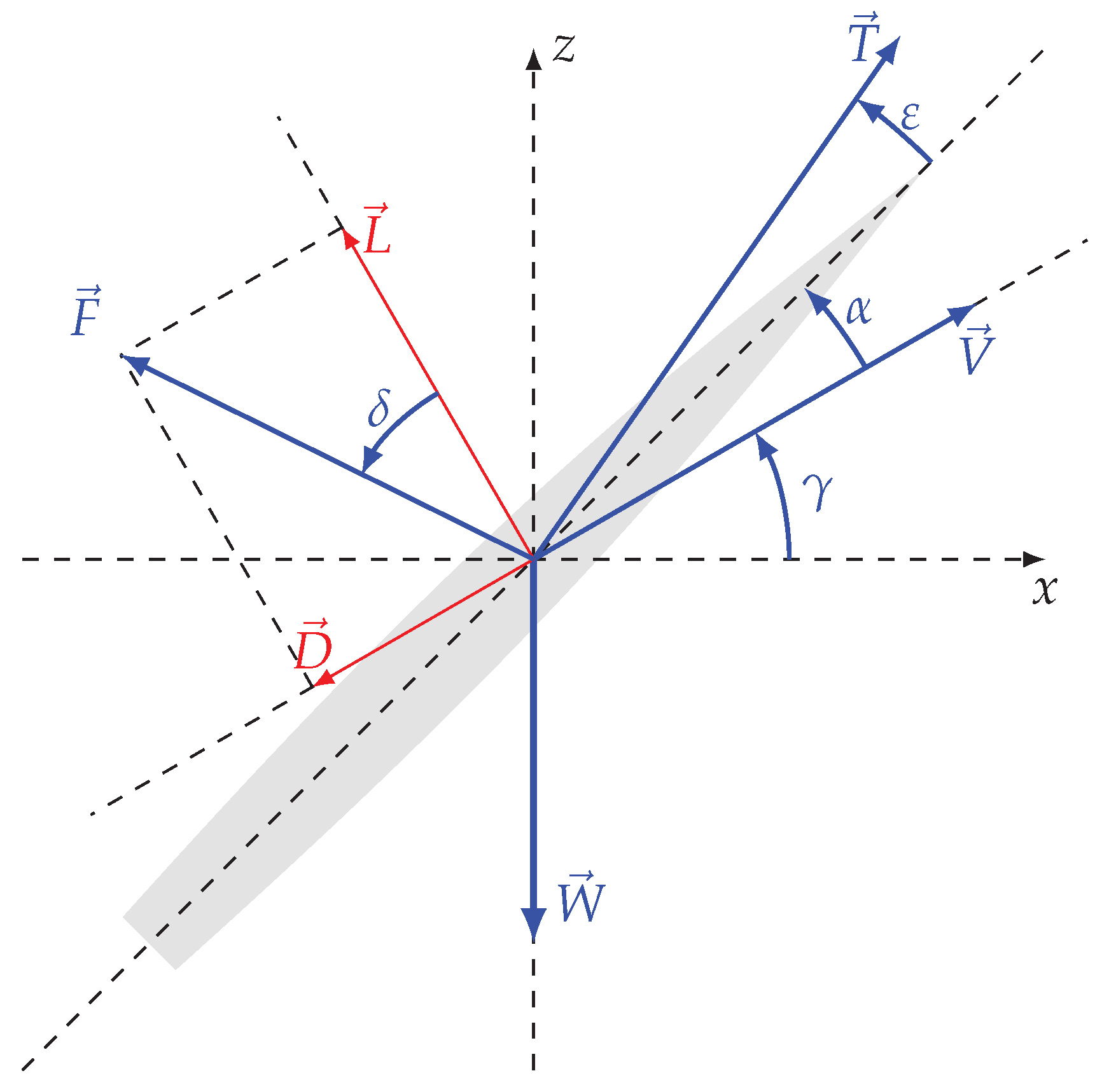
In the absence of aerodynamic or propulsive side force, and omitting the Coriolis force, the rocket trajectory lies on a plane. Two choices of coordinate systems are the most common: (a) a Cartesian earth-fixed coordinate frame; (b) an orthogonal Frenet–Serret frame moving along the trajectory with a longitudinal coordinate tangent to it, and hence the transversal coordinate towards or away from the center of curvature. Using the moving frame (b) and taking as variables the velocity and flight path angle, the acceleration components along and across the flight path are nonlinear; however, in this case, it is straightforward to eliminate time from the trajectory by dividing the longitudinal by the transversal acceleration, leading to a single differential equation for the path. This method was originally applied [6] to calculate the ballistic trajectory of a projectile of constant mass in a uniform gravity field, with drag proportional to a power of the velocity and opposite to it; the extension of this solution to include the effects of thrust and variable mass has been researched extensively [7,8]. The simplicity of this method is lost if the dependence of aerodynamic forces on altitude through the mass density is included; in this case, altitude appears explicitly in the equations of the trajectory, requiring an additional integral equation, without which its solution is not closed. The original method (a) can still be applied by altitude “steps” with constant density.

The present paper aims at including the continuous dependence of aerodynamic forces on altitude through the mass density, and chooses as a starting point the dynamical trajectory equations (Section 2), using an earth-fixed Cartesian frame (Section 2.3) rather than the orthogonal frame moving along the trajectory (Section 2.1); in the latter case, altitude can be eliminated (Section 2.2) by introducing the radius of the curvature of the trajectory. The use of fixed rather than a moving reference frame leads to two rather than one differential equation for the trajectory (Section 3). The problem is reduced to a single differential equation (Section 3.1) by the assumption of constant flight path angle. This rather restrictive assumption is used to develop more simply a one-dimensional method of solution (Section 3.2), specifying the altitude as a function of time (Section 3.3). A particular case of trajectory with a constant flight path angle is the vertical climb, which is quite inefficient at gaining speed because it works entirely against gravity; for this reason, the gravity turn is used [1,2,3,4,5] which could be approximated by a sequence of straight paths, each with a constant flight path angle. This restriction will be removed in subsequent work, where a continuous gravity turn is considered, using an extended variant of the methods developed here, in order to determine the curved two-dimensional trajectory, by specifying the horizontal and vertical coordinates and velocities as functions of time.

Two methods of solution of the equations of motion are considered, both using the atmospheric mass density as altitude variable; the time variable is: (Section 3) the burned propellant mass fraction in method I; and (Section 4) the residual mass fraction in method II. Both methods involve the same dimensionless thrust, gravity and drag parameters (Section 3.1 and Section 4.1), and use series expansions (Section 3.2 and Section 4.2), whose leading terms are calculated explicitly (Section 3.3 and Section 4.3). It is shown that method II is (Section 5.1) more accurate for a long time, e.g., burn-out, and method I for a short time, e.g., initial climb. Since method I has a more tedious algebra than method II, an alternative method III most suited for a short time is presented (Section 5.2) using a Taylor series of altitude as a function of time. All three methods apply to all stages of a multi-stage rocket, since they allow arbitrary initial altitude and velocity. The case of free flight without thrust post burnout is considered by a fourth method IV, extending the known solution for constant atmospheric mass density [3], to exponential variation of altitude; this method leads to a series expansion with the terms of all orders calculated explicitly (Section 5.3).

2. Dynamical Equations of the Rocket Trajectory

The dynamical equations of the rocket trajectory are written in two reference frames: (i) an earth-fixed Cartesian frame (Section 2.3) for which the components of acceleration and gravity are simplest; (ii) a moving Frenet–Serret orthogonal frame with one axis tangent to the trajectory at rocket velocity. In the latter case (ii), two possibilities are considered, viz: (ii-a) eliminating time (Section 2.1), in which case the altitude remains in the mass density in the aerodynamic forces; (ii-b) eliminating the atmospheric mass density (Section 2.2) by using the lift-to-drag ratio, in which case the radius of curvature of the trajectory appears.

2.1. Orthogonal Frame Moving with the Velocity

The geometry of a rocket trajectory (Figure 1) may be used to establish the equations of motion in an orthogonal frame, with one axis tangent to the trajectory, moving at the rocket velocity. The tangential Equation (1a) and normal Equation (1b) force balance are specified [9,10] respectively by:

$$\begin{array}{cc}\hfill m\frac{\mathrm{d}V}{\mathrm{d}t}& =-mgsin\gamma -Dcos\alpha -Lsin\alpha +Tcos(\alpha +\epsilon ),\hfill \end{array}$$

(1a)

$$\begin{array}{cc}\hfill mV\frac{\mathrm{d}\gamma }{\mathrm{d}t}& =-mgcos\gamma -Dsin\alpha +Lcos\alpha +Tsin(\alpha +\epsilon ),\hfill \end{array}$$

(1b)

where: (i) on the right-hand side, the inertia force is the product of the mass by the acceleration, whose tangential component involves only the total velocity V, whereas the normal component involves also the flight path angle $\gamma$; (ii) on the right-hand side. The first term is the gravity force, which is vertical downwards, and thus makes an angle $-\pi /2-\gamma$ with the velocity V, so that $cos(-\pi /2-\gamma )=-sin\gamma$ appears in Equation (1a) and $sin(-\pi /2-\gamma )=-cos\gamma$ appears in Equation (1b); (ii) the second term is the drag force D, which makes an angle $\pi +\alpha$ with the velocity, where $\alpha$ is the angle-of-attack, so that $cos(\pi +\alpha )=-cos\alpha$ appears in Equation (1a) and $sin(\pi +\alpha )=-sin\alpha$ appears in Equation (1b); (iii) the third term is the lift force L, which is orthogonal to the drag, and makes an angle $\pi /2+\alpha$ with the velocity, so that $cos(\pi /2+\alpha )=-sin\alpha$ appears in Equation (1a) and $sin(\pi /2+\alpha )=cos\alpha$ appears in Equation (1b); (iv) the last term is the thrust T, which makes an angle $\epsilon$ with the rocket axis, hence an angle $\alpha +\epsilon$ with the velocity, so that $cos(\alpha +\epsilon )$ appears in Equation (1a) and $sin(\alpha +\epsilon )$ in Equation (1b).

Of the coefficients in the equations of motion: (i) the mass m varies with time due to propellant consumption, e.g., for a constant flow rate is given by

$$-c\equiv \frac{\mathrm{d}m}{\mathrm{d}t}=\mathrm{const}.:m\left(t\right)=m_0-c(t-t_0),$$

(2a)

where the initial $m_0$ and final $m_1$ mass determine the burn time $t_1$,

$$t_0⩽t⩽t_1:t_1-t_0=\frac{m_0-m_1}{c},$$

(2b)

after which the trajectory is unpowered; (ii) this implies that the thrust T is zero for $t>t_1$, and before it is constant and non-zero if the effect of atmospheric pressure on nozzle expansion ratio is neglected, otherwise it is a function of altitude $T\left(z\right)$; (iii) the acceleration of gravity may be taken as constant for altitudes much smaller than the Earth radius $z_1-z_0\ll R=6378 \mathrm{k}\mathrm{m}$; and (iv) the remaining forces in Equations (1a,b) are lift and drag:

$$\begin{array}{c}L=\frac{1}{2}\rho \left(z\right)S{(V-u)}^2{C}_{\mathrm{L}}\left(\alpha \right),\end{array}$$

(3a)

$$\begin{array}{c}D=\frac{1}{2}\rho \left(z\right)S{(V-u)}^2{C}_{\mathrm{D}}\left(\alpha \right),\end{array}$$

(3b)

where the dimensionless lift $C_{\mathrm{L}}$ and drag $C_{\mathrm{D}}$ coefficients depend on the angle of attack $\alpha$ but not the cross-section S; in the simplest case, if weakly affected by the Mach and Reynolds numbers, they are independent of velocity V and mass density $\rho$, which thus appear respectively quadratically and linearly in the aerodynamic forces Equations (3a,b); the wind speed u projected along the tangent to the flight path is subtracted from the velocity V in an Earth fixed reference frame to specify the airspeed $V-u$ in the aerodynamic forces, namely lift Equation (3a) and drag Equation (3b); the atmospheric mass density decays rapidly with altitude, viz. exponentially with scale height ℓ

$${\rho }_0\equiv \rho \left(z_0\right):\rho \left(z\right)={\rho }_{0}exp\left(-\frac{z-z_0}{\ell }\right),$$

(4)

for an isothermal atmospheric layer.

Substituting Equation (4) in Equations (3a,b), the equations of motion (1a,b) become, with the preceding assumptions:

$$\begin{array}{cc}\hfill \left[m_0-c(t-t_0)\right]\frac{\mathrm{d}V}{\mathrm{d}t}& =-(m_0-ct)gsin\gamma +T\left(z\right)cos(\alpha +\epsilon )\hfill \\ & -\frac{1}{2}S{(V-u)}^2{\rho }_0{\mathrm{e}}^{-(z-z_0)/\ell }\left[C_{\mathrm{D}}\left(\alpha \right)cos\alpha +C_{\mathrm{L}}\left(\alpha \right)sin\alpha \right],\hfill \end{array}$$

(5a)

$$\begin{array}{cc}\hfill \left[m_0-c(t-t_0)\right]V\frac{\mathrm{d}\gamma }{\mathrm{d}t}& =-(m_0-ct)gcos\gamma +T\left(z\right)cos(\alpha +\epsilon )\hfill \\ & +\frac{1}{2}S{(V-u)}^2{\rho }_0{\mathrm{e}}^{-(z-z_0)/\ell }\left[C_{\mathrm{L}}\left(\alpha \right)cos\alpha -C_{\mathrm{D}}\left(\alpha \right)sin\alpha \right],\hfill \end{array}$$

(5b)

which are: (i) nonlinear because of the normal acceleration and aerodynamic forces; (ii) have coefficients depending on time through the mass varying with propellant consumption, and also possibly thrust vectoring $\epsilon \left(t\right)$ and angle-of-attack variation $\alpha \left(t\right)$ for flight control; (iii) the coefficients depend on altitude, through the atmospheric mass density in the aerodynamic forces, and nozzle pressure ratio in the thrust; and (iv) the wind speed is a local weather variable depending on time or altitude along the flight path.

If the angle-of-attack is zero $\alpha =0$, the thrust is aligned with the rocket axis $\epsilon =0$, and lift is neglected compared to drag $L\ll D$, then the equations of motion (1a,b) simplify to:

$$\begin{array}{cc}\hfill \alpha =0=\epsilon ,L\ll D:m\frac{\mathrm{d}V}{\mathrm{d}t}=& -mgsin\gamma +T-D,\hfill \end{array}$$

(6a)

$$\begin{array}{cc}\hfill mV\frac{\mathrm{d}\gamma }{\mathrm{d}t}=& -mgcos\gamma ,\hfill \end{array}$$

(6b)

which have been considered extensively in the literature [1,2,3,4,5]; eliminating $\mathrm{d}t$ by taking the ratio leads to

$$\frac{1}{V}\frac{\mathrm{d}V}{\mathrm{d}\gamma }=tan\gamma +\frac{D}{mg}sec\gamma -\frac{T}{mg}sec\gamma ,$$

(7)

which is a nonlinear differential equation relating the velocity V and flight path angle $\gamma$. The latter can be generalized by taking the ratio of Equations (1a,b), viz.

$$\frac{1}{V}\frac{\mathrm{d}V}{\mathrm{d}\gamma }=\frac{Tcos(\alpha +\epsilon )-mgsin\gamma -Dcos\alpha -Lsin\alpha }{Tsin(\alpha +\epsilon )-mgcos\gamma -Dsin\alpha +Lcos\alpha }.$$

(8)

Even if the angle-of-attack $\alpha \left(t\right)$ and thrust vector angle $\epsilon \left(t\right)$ are constant in Equation (8), or zero in Equation (7), the time dependence remains in the mass $m\left(t\right)$, e.g., Equations (2a,b) for constant rate of propellant consumption. The altitude dependence remains in Equation (8) through the thrust being a function of nozzle pressure ratio and aerodynamic forces depending on mass density; even for constant thrust and zero lift in Equation (7), the altitude still appears through the atmospheric mass density Equation (4) in the drag force Equation (3a). The altitude z is related to the velocity and flight path angle via an integration over time,

$$z-z_0={\int }_{t_0}^{t}V\left(t\right)sin\gamma \left(t\right)\mathrm{d}t.$$

(9)

The inclusion of Equation (9) in the mass density Equation (4) through the aerodynamic forces Equations (3a,b), turn Equation (7) or Equation (8) into an integro-differential equation for $V,\gamma$. This could be avoided by approximating Equation (7) or Equation (8) as a sequence of altitude steps with constant density, along the rocket trajectory (Figure 2).

2.2. Influence of the Lift-to-Drag Ratio

The altitude dependence could be eliminated from the coefficients of the general equations of motion (1a,b) in the form:

$$\begin{array}{cc}\hfill Dcos\alpha +Lsin\alpha & =Tcos(\alpha +\epsilon )-mgsin\gamma -m\frac{\mathrm{d}V}{\mathrm{d}t},\hfill \end{array}$$

(10a)

$$\begin{array}{cc}\hfill Dsin\alpha -Lcos\alpha & =Tsin(\alpha +\epsilon )-mgcos\gamma -m\frac{\mathrm{d}\gamma }{\mathrm{d}t},\hfill \end{array}$$

(10b)

by dividing to obtain

$$\frac{\lambda +tan\alpha }{\lambda tan\alpha -1}=\frac{Tcos(\alpha +\epsilon )-mgsin\gamma -m\frac{\mathrm{d}V}{\mathrm{d}t}}{Tsin(\alpha +\epsilon )-mgcos\gamma -m\frac{\mathrm{d}\gamma }{\mathrm{d}t}},$$

(11)

where the aerodynamic forces appear only through the drag-to-lift ratio

$$\lambda \equiv \frac{D}{L}=\frac{C_{\mathrm{D}}\left(\alpha \right)}{C_{\mathrm{L}}\left(\alpha \right)}=\frac{C_{\mathrm{D}0}}{C_{\mathrm{L}}\left(\alpha \right)}+\overline{K}+K{C}_{\mathrm{L}}\left(\alpha \right),$$

(12)

the latter is independent of velocity and wind speed, and also of mass density and hence also altitude. Thus, for constant thrust, the altitude is eliminated from Equation (11), and the drag-to-lift ratio Equation (12) depends only on angle-of-attack, e.g., in the simplest case it involves, besides the lift coefficient $C_{\mathrm{L}}\left(\alpha \right)$ the: (i) friction drag coefficient $C_{\mathrm{D}0}$; (ii) the lift-induced drag coefficient K; and (iii) the coefficient $\overline{K}$ for quadratic non-parabolic lift-drag polar. Writing the drag-to-lift ratio in terms of an aerodynamic angle $\delta$ in Equation (13a):

$$\begin{array}{cc}\hfill \lambda \equiv \frac{D}{L}& =tan\delta ,\hfill \end{array}$$

(13a)

$$\begin{array}{cc}\hfill \frac{\lambda +tan\hspace{0.17em}\alpha }{\lambda tan\hspace{0.17em}\alpha -1}& =tan(\alpha +\delta ),\hfill \end{array}$$

(13b)

and the left-hand side of Equation (11) takes the form Equation (13b). Figure 1 shows the rocket axis making an angle-of-attack $\alpha$ with the velocity vector $\overrightarrow{V}$, and the lift L and drag D components of the total aerodynamic force $\overrightarrow{F}$; the aerodynamic angle $\delta$ is the angle of the total aerodynamic force with the lift, and appears to be added to the angle-of-attack in Equation (13b), the left-hand side of the equation of the trajectory (11).

On the right-hand side of Equation (11), the differential of time $\mathrm{d}t$ can be eliminated by using the arc length $\mathrm{d}s$ and the radius of curvature Equation (14a) of the trajectory viz.:

$$\begin{array}{cc}\hfill R& =\frac{\mathrm{d}s}{\mathrm{d}\gamma },\hfill \end{array}$$

(14a)

$$\begin{array}{cc}\hfill V\frac{\mathrm{d}\gamma }{\mathrm{d}t}& =V\frac{\mathrm{d}\gamma }{\mathrm{d}s}\frac{\mathrm{d}s}{\mathrm{d}t}=\frac{V^2}{R},\hfill \end{array}$$

(14b)

in the normal Equation (14b) and tangential Equation (14c) acceleration,

$$\frac{\mathrm{d}V}{\mathrm{d}t}=\frac{\mathrm{d}V}{\mathrm{d}\gamma }\frac{\mathrm{d}\gamma }{\mathrm{d}s}\frac{\mathrm{d}s}{\mathrm{d}t}=\frac{V}{R}\frac{\mathrm{d}V}{\mathrm{d}\gamma }.$$

(14c)

Substituting Equations (14b,c) in Equation (11) leads to an equation for the trajectory,

$$tan(\alpha +\delta )=\frac{\lambda +tan\alpha }{\lambda tan\alpha -1}=\frac{Tcos(\alpha +\epsilon )-mgsin\gamma -m\frac{V}{R}\frac{\mathrm{d}V}{\mathrm{d}\gamma }}{Tsin(\alpha +\epsilon )-mgcos\gamma -m\frac{V^2}{R}},$$

(15)

which also involves the velocity V and flight path angle $\gamma$ like Equation (8) but eliminates dependence on altitude, and quadratic terms on the velocity and wind speed in the aerodynamic forces.

Using the simplifying assumptions as in Equations (6a,b) of zero angle-of-attack and thrust vector angle, and negligible lift, simplifies Equation (15) to

$$\alpha =0=\epsilon ,L\ll D:tan(\alpha +\delta )=\frac{\lambda +tan\alpha }{\lambda tan\alpha -1}=\frac{V\frac{\mathrm{d}V}{\mathrm{d}\gamma }+gRsin\gamma -\frac{RT}{m}}{V^2+gRcos\gamma },$$

(16)

which should be compared with Equation (7), just as the more general forms, respectively Equations (15) and (8), can be compared: (i) both are first-order nonlinear differential equations for the velocity V and flight path angle $\gamma$; (ii) the coefficients depend on time in both because of variable mass $m\left(t\right)$ in Equations (7) and (16), and possibly also thrust vectoring $\epsilon \left(t\right)$ and angle-of-attack scheduling $\alpha \left(t\right)$ in Equations (8) and (15).

The differences are that: (i) the altitude appears explicitly in Equations (7) and (8), even at constant thrust, leading by Equation (9) to an integro-differential equation; (ii) the altitude does not appear in Equations (15) or (16) for constant thrust, but the radius of curvature Equation (14a) appears, viz.

$$R=\frac{\mathrm{d}s}{\mathrm{d}\gamma }=\frac{\frac{\mathrm{d}s}{\mathrm{d}t}}{\frac{\mathrm{d}\gamma }{\mathrm{d}t}}=\frac{V}{\dot{\gamma }},$$

(17)

the radius of curvature is the ratio of the velocity to the angular velocity of the flight path angle. The radius of curvature is a function of the arc length $R\left(s\right),$ which is related to the velocity in the absence of wind by

$$s={\int }_0^t{\left[V\left(t\right)\right]}^{-1}\mathrm{d}t,$$

(18)

and substitution of Equation (18) in Equation (15) or Equation (16) leads an to integro-differential equation. This can be avoided by approximating the trajectory by circular arcs, which have constant radius of curvature (Figure 3); the flight path angle can be made continuous at the junction of two circular arcs, by choosing the center at the intersection of the normals at the end-points.

2.3. Fixed Cartesian Frame with Axis Along Altitude

In an earth-fixed Cartesian frame with a z-axis along the altitude and the x-axis down range, the acceleration is linear in the equations of motion:

$$\begin{array}{cc}\hfill m\ddot{x}=& -Dcos(\gamma +\alpha )-Lsin(\gamma +\alpha )+Tcos(\gamma +\alpha +\epsilon ),\hfill \end{array}$$

(19a)

$$\begin{array}{cc}\hfill m\ddot{z}=& -mg-Dsin(\gamma +\alpha )+Lcos(\gamma +\alpha )+Tsin(\gamma +\alpha +\epsilon ),\hfill \end{array}$$

(19b)

and the acceleration of gravity appears as a constant and only in one equation; the remaining forces, viz. thrust, lift and drag are similar in Equations (1a,b) and (19a,b), with the flight path angle $\gamma$ added in all trigonometric coefficients. The aerodynamic forces Equations (3a,b) can be written Equations (20a,b) in the absence of wind [11,12]:

$$\begin{array}{cc}\hfill L& =\frac{1}{2}\rho \left(z\right)S({\dot{x}}^2+{\dot{z}}^2)C_{\mathrm{L}}\left(\alpha \right),\hfill \end{array}$$

(20a)

$$\begin{array}{cc}\hfill D& =\frac{1}{2}\rho \left(z\right)S({\dot{x}}^2+{\dot{z}}^2)C_{\mathrm{D}}\left(\alpha \right),\hfill \end{array}$$

(20b)

and using the same assumptions Equations (2a,b) and (4) as before, the equations of motion (19a,b) become:

$$\begin{array}{cc}\hfill \left[m_0-c(t-t_0)\right]\ddot{x}& =Tcos(\gamma +\alpha +\epsilon )-\frac{1}{2}{\rho }_{0}S\left({\dot{x}}^2+{\dot{z}}^2\right){\mathrm{e}}^{-(z-z_0)/\ell }\hfill \\ & \times \left[C_{\mathrm{D}}\left(\alpha \right)cos(\gamma +\alpha )+C_{\mathrm{L}}\left(\alpha \right)sin(\gamma +\alpha )\right],\hfill \end{array}$$

(21a)

$$\begin{array}{cc}\hfill \left[m_0-c(t-t_0)\right](\ddot{z}+g)& =Tsin(\gamma +\alpha +\epsilon )-\frac{1}{2}{\rho }_{0}S\left({\dot{x}}^2+{\dot{z}}^2\right){\mathrm{e}}^{-(z-z_0)/\ell }\hfill \\ & \times \left[C_{\mathrm{D}}\left(\alpha \right)sin(\gamma +\alpha )-C_{\mathrm{L}}\left(\alpha \right)cos(\gamma +\alpha )\right],\hfill \end{array}$$

(21b)

where the flight path angle

$$tan\gamma =\frac{\mathrm{d}z}{\mathrm{d}x}=\frac{\dot{z}}{\dot{x}}$$

(22)

must be substituted.

The substitution of the flight path angle in the equations of motion (21a,b) is made using:

$$\begin{array}{cc}\hfill cos\gamma & ={\left|{\dot{x}}^2+{\dot{z}}^2\right|}^{-1/2}\dot{x},\hfill \end{array}$$

(23a)

$$\begin{array}{cc}\hfill sin\gamma & ={\left|{\dot{x}}^2+{\dot{z}}^2\right|}^{-1/2}\dot{z},\hfill \end{array}$$

(23b)

in:

$$\begin{array}{cc}\hfill {\left|{\dot{x}}^2+{\dot{z}}^2\right|}^{1/2}cos(\gamma +\alpha )& =\dot{x}cos\alpha -\dot{z}sin\alpha ,\hfill \end{array}$$

(24a)

$$\begin{array}{cc}\hfill {\left|{\dot{x}}^2+{\dot{z}}^2\right|}^{1/2}sin(\gamma +\alpha )& =\dot{x}sin\alpha +\dot{z}cos\alpha ,\hfill \end{array}$$

(24b)

and likewise for $cos,sin(\gamma +\alpha +\epsilon )$ replacing $\alpha$ by $\alpha +\epsilon$. Thus, the equations of motion (21a,b) in Cartesian coordinates Equations (24a,b) become

$$\begin{array}{c}[m_0-c(t-t_0)]{\left|{\dot{x}}^2+{\dot{z}}^2\right|}^{1/2}\left[\begin{array}{c}\ddot{x}\\ \ddot{z}+g\end{array}\right]=T\left(z\right)\left[\begin{array}{cc}cos(\alpha +\epsilon )& -sin(\alpha +\epsilon )\\ sin(\alpha +\epsilon )& cos(\alpha +\epsilon )\end{array}\right]\left[\begin{array}{c}\dot{x}\\ \dot{z}\end{array}\right]\hfill \\ -\frac{1}{2}{\rho }_{0}Sexp[-(z-z_0)/\ell ]\left({\dot{x}}^2+{\dot{z}}^2\right)\left[\begin{array}{cc}{C}_{\mathrm{D}}cos\alpha +C_{\mathrm{L}}sin\alpha & -C_{\mathrm{D}}sin\alpha +C_{\mathrm{L}}cos\alpha \\ C_{\mathrm{D}}sin\alpha -C_{\mathrm{L}}cos\alpha & C_{\mathrm{D}}cos\alpha +C_{\mathrm{L}}sin\alpha \end{array}\right]\left[\begin{array}{c}\dot{x}\\ \dot{z}\end{array}\right].\hfill \end{array}$$

(25)

The time dependence appears in the mass, angle-of-attack $\alpha$ and thrust vector angle $\epsilon$; the altitude dependence appears in the atmospheric mass density and thrust.

The trajectory can be approximated by at least three alternative methods: (i) altitude steps (Figure 2) of constant atmospheric mass density (Section 2.1); (ii) circular arcs (Figure 3) of constant radius of curvature (Section 2.2); and (iii) straight segments with a constant flight path angle (Figure 4). This approximation will be released in subsequent work, and is used next to develop more simply a method of trajectory calculation. The assumption of constant flight path angle $\gamma$ in Equation (22) implies that the trajectory is specified by one equation only, e.g., Equation (21b) for altitude:

$$\begin{array}{c}\left[m_0-c(t-t_0)\right](\ddot{z}+g)=T\left(z\right)sin(\gamma +\alpha +\epsilon )+\frac{1}{2}{\rho }_{0}S{\dot{z}}^2{csc}^2\gamma exp[-(z-z_0)/\ell ]\\ \times \left[C_{\mathrm{L}}\left(\alpha \right)cos(\gamma +\alpha )-C_{\mathrm{D}}\left(\alpha \right)sin(\gamma +\alpha )\right],\end{array}$$

(26)

which allows for vertical flight $\gamma =\pi /2$ but excludes horizontal flight $\gamma =0$. The opposite would be the case choosing Equation (21a).

The flight path angle can be taken as constant only if the vertical and horizontal accelerations are also in the ratio Equation (22), viz.

$$\ddot{x}sin\gamma =\ddot{z}cos\gamma .$$

(27)

Substituting Equations (19a,b) in Equation (27) leads to the identity

$$mgcos\gamma +Dsin\alpha =Lcos\alpha +Tsin(\alpha +\epsilon ),$$

(28)

which states (Figure 1) the balance of forces normal to the flight path. In particular, vertical flight $\gamma =\pi /2$ or $cos\gamma =0$ is possible for zero angle of attack $\alpha =0$, thrust aligned with the rocket axis $\epsilon =0$ and negligible lift $L=0$. If the angle of attack is zero $\alpha =0$ and lift is neglected $L=0$, then thrust at angle $\epsilon \ne 0$ to the rocket axis would lead to a trajectory at an angle $\pi /2-\gamma$ to the vertical, with flight path angle

$$\alpha =0=L:cos\gamma =\frac{T}{mg}sin\epsilon ,$$

(29)

which would be constant for constant mass and fixed thrust angle, or mass variation compensated by thrust vectoring. In general, the aerodynamic forces vary with velocity and altitude in Equation (28), and rocket mass changes with time, so that a constant flight path angle could be maintained by thrust modulation or vectoring or angle-of-attack scheduling. In this case, Equation (28) could be used together with the equation of motion tangent to the trajectory,

$$m\ddot{z}csc\gamma =-mgsin\gamma +Tsin(\alpha +\epsilon )+Lcos\alpha -Dsin\alpha ,$$

(30a)

or alternatively:

$$\begin{array}{c}\left[m_0-c(t-t_0)\right]\ddot{z}csc\gamma =-mgsin\gamma +T\left(z\right)sin(\alpha +\epsilon )\hfill \\ +\frac{1}{2}{\rho }_{0}S{\dot{z}}^2{csc}^2\gamma exp[-(z-z_0)/\ell ]\left[C_{\mathrm{L}}\left(\alpha \right)cos\alpha -C_{\mathrm{D}}\left(\alpha \right)sin\alpha \right],\hfill \end{array}$$

(30b)

with the assumptions Equations (2a), (3a,b), and (4).

3. Trajectory Calculation via a Power Series of Time

The method of trajectory calculation using power series of the time is presented most simply for a vertical climb, which involves only three dimensionless parameters representing gravity, thrust and drag (Section 3.1); the ratio of atmospheric mass densities at arbitrary altitude z relative to initial altitude $z_0$ is used as a dimensionless altitude variable, and the time is made dimensionless using the initial mass and propellant rate (Section 3.2); the nonlinear differential equation and initial conditions determine the leading coefficients of a power series solution.

3.1. Dimensionless Gravity, Thrust and Drag Parameters

For zero angle-of-attack $\alpha =0$, neglecting lift $L=0$, and thrust aligned with the rocket axis, the condition Equation (28) of a straight flight path is met for $cos\gamma =0$ or $\gamma =\pi /2$, i.e., a vertical climb, in which case Equation (30a) simplifies to

$$\alpha =\epsilon =0=L:m\ddot{z}=-mg+T-D,$$

(31)

which balances the inertia force against gravity, thrust and drag, leading in the absence of wind to

$$\left[m_0-c(t-t_0)\right](\ddot{z}+g)=T-\frac{1}{2}{C}_{\mathrm{D}}S{\rho }_0{\dot{z}}^{2}exp[-(z-z_0)/\ell ],$$

(32)

using the assumptions Equations (2a,3b,4). The initial altitude is taken to be $z_0$ at time $t=t_0$ so that the results can be applied to any stage of a multistage rocket. Thus, the differential equation is solved with the initial conditions:

$$\begin{array}{c}\hfill z\left(t_0\right)=z_0,\end{array}$$

(33a)

$$\begin{array}{c}\hfill \dot{z}\left(t_0\right)=v_0,\end{array}$$

(33b)

specifying altitude Equation (33a) and velocity Equation (33b) at time $t=t_0$ of thrust initiation for an upper stage, or lift-off for the first stage.

Next, dimensionless independent and dependent variables are introduced. The dependent variable is altitude, z, which is taken relative to initial altitude, made dimensionless Equation (34a) by dividing by the atmospheric scale height:

$$\begin{array}{cc}\hfill \zeta & \equiv (z-z_0)/\ell ,\hfill \end{array}$$

(34a)

$$\begin{array}{cc}\hfill \tau & \equiv \frac{m\left(t\right)}{m_0}-1=\frac{c(t-t_0)}{m_0},\hfill \end{array}$$

(34b)

whereas time is replaced as the independent variable by Equation (34b) the ratio of the mass of propellant burned $c(t-t_0)$ to the initial mass $m_0$. Substituting Equations (34a,b) in the equation of motion (32), it takes the dimensionless form

$$(1-\tau )\left({\zeta }^{″}+a\right)=b-f{\zeta }^{\prime 2}{\mathrm{e}}^{-\zeta },$$

(35)

where prime denotes derivative with regard to $\tau$, viz. ${\zeta }^{\prime }=\frac{\mathrm{d}\zeta }{\mathrm{d}\tau }$, and the three parameters:

$$\begin{array}{cc}\hfill a& \equiv \frac{m_0^{2}g}{c^2\ell },\hfill \end{array}$$

(36a)

$$\begin{array}{cc}\hfill b& \equiv \frac{m_{0}T}{c^2\ell },\hfill \end{array}$$

(36b)

$$\begin{array}{cc}\hfill f& \equiv \frac{C_{\mathrm{D}}{\rho }_{0}S\ell }{2m_0},\hfill \end{array}$$

(36c)

are also all dimensionless.

The dimensionless parameters specify the relative importance of gravity Equation (36a), thrust Equation (36b), and drag Equation (36c), which are in the proportion

$$m_{o}g:T:\frac{C_{\mathrm{D}}}{2}\frac{{\rho }_{0}S\ell }{m_0}\frac{c^2\ell }{m_0}.$$

(37)

The last term in Equation (37) involves the reference mass $m_{*}$ defined by Equation (38a) as the mass of a column of air, with the mass density ${\rho }_0$ at the initial altitude $z_0$, height equal to the atmospheric scale height ℓ, and cross-section S equal to that of the rocket:

$$\begin{array}{cc}\hfill m_{*}& ={\rho }_{0}S\ell ,\hfill \end{array}$$

(38a)

$$\begin{array}{cc}\hfill f& =\frac{C_{\mathrm{D}}}{2}\frac{m_{*}}{m_0},\hfill \end{array}$$

(38b)

the dimensionless drag parameter Equation (36c) equals Equation (38b) the reference mass normalized to the initial mass $m_{*}/m_0$, multiplied by half the drag coefficient. The dimensionless acceleration Equation (36a) is the ratio Equation (38c) of the acceleration of gravity g to the reference acceleration Equation (38d):

$$\begin{array}{cc}\hfill a& \equiv \frac{g}{a_{*}},\hfill \end{array}$$

(38c)

$$\begin{array}{cc}\hfill a_{*}& =\frac{c^2\ell }{m_0^2},\hfill \end{array}$$

(38d)

which is an acceleration constructed from the propellant rate Equation (2a), initial $m_0$ and atmospheric scale height ℓ in Equation (4). The dimensionless thrust parameter Equation (36b) is similar to Equation (36a) replacing the initial rocket weight $m_{0}g$ bt the thrust T.

3.2. Atmospheric Mass Density as a Function of the Mass of Burned Propellant

In order to eliminate the exponential nonlinearity from the differential equation of motion (35), the initial atmospheric mass density ${\rho }_0$ at altitude $z_0$, divided by the mass density $\rho$ at altitude z, is taken instead of the dimensionless relative altitude Equation (34a), as the dependent variable

$$\eta \equiv \frac{{\rho }_0}{\rho \left(z\right)}=exp\left[\frac{z-z_0}{\ell }\right]={\mathrm{e}}^{\zeta };$$

(39)

this implies:

$$\begin{array}{cc}\hfill {\zeta }^{\prime }& ={(log\eta )}^{\prime }=\frac{{\eta }^{\prime }}{\eta },\hfill \end{array}$$

(40a)

$$\begin{array}{cc}\hfill {\zeta }^{″}& =\frac{{\eta }^{″}}{\eta }-{\left(\frac{{\eta }^{\prime }}{\eta }\right)}^2,\hfill \end{array}$$

(40b)

so that the exponential nonlinearity in the equation of motion (35) is replaced by algebraic nonlinearities

$$(1-\tau )\eta \left(\eta {\eta }^{″}-{\eta }^{\prime 2}+a{\eta }^2\right)-b{\eta }^3=-f{\eta }^{\prime 2},$$

(41)

viz. quadratic for the drag term on the right-hand side of Equation (41) and cubic for all other terms on the left-hand side of Equation (41), viz. inertia, gravity, and thrust. This will imply that drag effects will first appear at higher order than inertia, gravity and thrust.

The solution of the nonlinear differential equation (41) will be sought as a power series

$$\eta \left(\tau \right)=\sum _{n=0}^{\infty }{A}_n{\tau }^{n+\upsilon },$$

(42)

with exponent $\upsilon$ and coefficients $A_n$ to be determined. Recalling Equations (39) and (34b), the trajectory is specified

$$exp\left[\frac{z-z_0}{\ell }\right]=\sum _{n=0}^{\infty }{A}_n{\left[\frac{c(t-t_0)}{m_0}\right]}^{\upsilon +n}$$

(43)

by altitude (represented by the ratio of initial mass density to varying atmospheric mass density) as a function of time (represented by burned propellant mass relative to initial mass). The condition Equation (33b) of initial altitude $z=z_0$ at time $t=t_0$, implies Equations (44a,b):

$$\begin{array}{cc}\hfill A_0& =1,\hfill \end{array}$$

(44a)

$$\begin{array}{cc}\hfill \upsilon & =0,\hfill \end{array}$$

(44b)

$$\begin{array}{cc}\hfill \eta \left(\tau \right)& =1+{\displaystyle \sum _{n=1}^{\infty }}{A}_n{\tau }^n,\hfill \end{array}$$

(44c)

specifying in Equation (44c) the exponent and first coefficient of Equation (42).

Using again Equations (34b) and (39), the trajectory Equation (44c) specifies:

$$exp\left(\frac{z-z_0}{\ell }\right)=1+\sum _{n=1}^{\infty }{A}_n{\left[\frac{c(t-t_0)}{m_0}\right]}^n,$$

(45)

and by differentiation with regard to time, the velocity $\dot{z}$ in:

$$\dot{z}exp\left(\frac{z-z_0}{\ell }\right)=\frac{c\ell }{m_0}\sum _{n=1}^{\infty }n{A}_n{\left[\frac{c(t-t_0)}{m_0}\right]}^{n-1}.$$

(46)

The initial condition Equation (33b) for the velocity $\dot{z}=v_0$ at time $t_0$ specifies the coefficient $A_1$:

$$\begin{array}{cc}\hfill v_0& =A_1\frac{c\ell }{m_0}=A_1{v}_{*},\hfill \end{array}$$

(47a)

$$\begin{array}{cc}\hfill v_{*}& \equiv \frac{c\ell }{m_0},\hfill \end{array}$$

(47b)

as the ratio of initial velocity $v_0$ to the reference velocity $v_{*}$, defined by Equation (47b). In order to interpret the latter note that the reference velocity $v_{*}$ corresponds Equation (48a) to a distance equal to the atmospheric scale height ℓ covered in a reference time $t_{*}$:

$$\begin{array}{cc}\hfill v_{*}& =\frac{\ell }{t_{*}},\hfill \end{array}$$

(48a)

$$\begin{array}{cc}\hfill t_{*}& \equiv \frac{m_0}{c}>t_1-t_0,\hfill \end{array}$$

(48b)

where the reference time is the initial rocket mass divided by the propellant burn rate; thus, the reference time would be the burn time if the rocket mass was entirely propellant, and must exceed the real burn time.

3.3. Leading Coefficients of Power Series Expansion

Using Equation (47a), the power series Equation (44c) for the trajectory becomes

$$\eta \left(\tau \right)=1+\frac{v_0}{v_{*}}\tau +\sum _{n=2}^{\infty }{A}_0{\tau }^n,$$

(49)

and is considered next up to order $N+2$; since the equation of motion (41) involves at most second-order derivatives, it becomes a polynomial of degree N in $\tau$ which is accurate only to order ${\tau }^N$ and whose coefficients involve $A_2,A_3,\dots ,A_{N+2}$; equating to zero the coefficients of the $N+2$ successive powers of $\tau$, viz. ${\tau }^0=1,\tau ,\dots ,{\tau }^{N+2}$ yields a set of $N+1$ nonlinear algebraic equations, which can be solved for the $N+1$ unknowns $A_2,\dots ,A_{N+2}$ since $A_0,A_1$ are already known from Equations (44a) and (47a). This process is illustrated by substituting the series solution for the trajectory Equation (49) for $N=2$, i.e., up to $N+2=4$ the fourth-order in $\tau$,

$$\eta \left(\tau \right)=1+\frac{v_0\tau }{v_{*}}+A_2{\tau }^2+A_3{\tau }^3+A_4{\tau }^4+O\left({\tau }^5\right),$$

(50)

into the Equation (41) up to order 2,

$$\begin{array}{c}-f{\left(\frac{v_0}{v_{*}}+2A_2\tau +3A_3{\tau }^2\right)}^2=-b{\left(1+\frac{v_0\tau }{v_{*}}+A_2{\tau }^2\right)}^3\hfill \\ +(1-\tau )\left(1+\frac{v_0\tau }{v_{*}}+A_2{\tau }^2\right)\left[\left(1+\frac{v_0\tau }{v_{*}}+A_2{\tau }^2\right)\left(2A_2+6A_3\tau +12A_4{\tau }^2\right)\right.\hfill \\ -\left.{\left(\frac{v_0}{v_{*}}+2A_2\tau +3A_3{\tau }^2\right)}^2+a{\left(1+\frac{v_0\tau }{v_{*}}+A_2{\tau }^2\right)}^2\right]+O\left({\tau }^3\right),\hfill \end{array}$$

(51)

which is valid only to $O\left({\tau }^3\right)$ because some cubic and higher-order terms were omitted.

Equating to zero the term of Equation (51) independent of $\tau$ specifies

$$2A_2=b-a+(1-f){(v_0/v_{*})}^2,$$

(52)

which is the coefficient of ${\tau }^2$ in Equation (50) of the trajectory. Equating to zero the coefficient of $\tau$ in the equation of motion (51) leads to:

$$6A_3=(3b-2a)\frac{v_0}{v_{*}}+2A_2(1-2f)\frac{v_0}{v_{*}}+\left(1-\frac{v_0}{v_{*}}\right)\left[2A_2+a-{\left(\frac{v_0}{v_{*}}\right)}^2\right],$$

(53a)

which on substitution of Equation (52) specifies the coefficient $A_3$ of ${\tau }^3$ in the Equation (50) of the trajectory, viz.,

$$6A_3=b+(b-a)(3-2f)\frac{v_0}{v_{*}}-f{\left(\frac{v_0}{v_{*}}\right)}^2+(1-2f+2f^2){\left(\frac{v_0}{v_{*}}\right)}^3.$$

(53b)

Equating to zero the coefficient of ${\tau }^2$ in the equation of motion (51) leads to

$$\begin{array}{c}12A_4=-2f\left[3A_3\left(\frac{v_0}{v_{*}}\right)+2A_2^2\right]+3b\left[A_2+{\left(\frac{v_0}{v_{*}}\right)}^2\right]\hfill \\ -3a\left[A_2-\left(1-\frac{v_0}{v_{*}}\right)\frac{v_0}{v_{*}}\right]+3A_2{\left(\frac{v_0}{v_{*}}\right)}^2\hfill \\ +6A_3\left(1-\frac{v_0}{v_{*}}\right)-{\left(\frac{v_0}{v_{*}}\right)}^3,\hfill \end{array}$$

(54)

which on substitution of $A_2,A_3$ from Equations (52, 53a) specifies the coefficient $A_4$ of ${\tau }^4$ in the equation of the trajectory (50), as a polynomial of degree four in $v_0/v_{*}$, with coefficients involving $a,b,f$. In a similar way, the vanishing of the coefficient of ${\tau }^N$ in the equation of motion (41), specifies the coefficient $A_{N+2}$ of ${\tau }^{N+2}$ in the equation of the trajectory (49); as can be seen from Equations (52, 53a, 54), the coefficient $A_{N+2}$ is a polynomial of $v_0/v_{*}$ of degree $N+2$, whose coefficients involve the dimensionless gravity Equation (36a) = Equations (38c,d), thrust Equation (36b), and drag Equation (36c) = Equations (38a,b) parameters.

4. Alternative Methods for Short Times or Long Times

The dimensionless time variable is taken to be, instead of mass fraction of burned propellant (Section 3), which increases with time, the residual mass fraction (Section 4), which reduces with time (Section 4.1), and is minimum at burn-out, and thus is most convenient to calculate burn-out altitude and velocity (Section 5), once the series solution (Section 4.2) has been determined (Section 4.3).

4.1. Residual Mass Fractions as Time Variable

The dimensionless time variable is taken to be, instead of mass fraction of burned propellant Equation (34b), the residual mass fraction

$$1⩾\mu \equiv m\left(t\right)/m_0=1-c(t-t_0)/m_0⩾m_1/m_0,$$

(55)

which varies from unity $\mu =1$ at initial time $t=t_0$ to the ratio of empty mass at burn-out to total initial mass, when it is usually much smaller than unity. Using the residual mass fraction Equation (55) as an independent variable, and the same dependent variable Equation (34a), the equation of motion (32) becomes

$$\mu \left({\zeta }^{″}+a\right)=b-f{\zeta }^{\prime 2}{\mathrm{e}}^{-\zeta },$$

(56)

instead of Equation (35), where prime now denotes derivative with regard to $\mu$, viz. ${\zeta }^{\prime }\equiv \mathrm{d}\zeta /\mathrm{d}\mu$, and the dimensionless gravity Equation (36a) ≡ Equations (38c,d), thrust Equation (36b) and drag Equation (36c) ≡ Equations (38a,b) coefficients are the same.

Since the independent variable, viz. the residual mass fraction decreases with time, the dependent variable should decrease with altitude, e.g., the inverse of Equation (39) is used, viz. the ratio of atmospheric mass density $\rho$ at altitude z to initial mass density ${\rho }_0$ at altitude $z_0$ is used:

$$\xi \equiv 1/\eta =\rho \left(z\right)/{\rho }_0=exp\left(-\frac{z-z_0}{\ell }\right)={\mathrm{e}}^{-\xi },$$

(57)

as dimensionless altitude variable. Bearing in mind that:

$$\begin{array}{cc}\hfill {\zeta }^{\prime }& =(-log\xi )=-\frac{{\xi }^{\prime }}{\xi },\hfill \end{array}$$

(58a)

$$\begin{array}{cc}\hfill {\zeta }^{″}& =-\frac{{\xi }^{″}}{\xi }+{\left(\frac{{\xi }^{\prime }}{\xi }\right)}^2,\hfill \end{array}$$

(58b)

the exponential nonlinearity in the equation of motion (56) is replaced by algebraic nonlinearities

$$-f{\xi }^{\prime 2}\xi =-b{\xi }^2+\mu (a{\xi }^2+{\xi }^{\prime 2}-{\xi }^{″}\xi ),$$

(59)

which are cubic for the drag term on the l.h.s. and quadratic for all the other terms on the right-hand side, viz. the thrust, gravity and inertia terms; this is the reverse of the situation before with Equation (41).

The solution of the equation of motion (59), i.e., the trajectory, is sought as the ratio of atmospheric mass densities Equation (52) expressed by a power series of residual mass fraction (55), viz.,

$$\xi =\sum _{n=0}^{\infty }{B}_n{\mu }^{n+\vartheta }$$

(60)

with exponent $\vartheta$ and coefficients $B_n$ to determined. The altitude is given explicitly Equation (57) as a function of time Equation (55) by

$$exp\left(-\frac{z-z_0}{\ell }\right)=\sum _{n=0}^{\infty }{B}_n{\left[1-\frac{c(t-t_0)}{m_0}\right]}^{n+\vartheta },$$

(61)

and the velocity is obtained by differentiation with regard to time

$$\dot{z}exp\left(-\frac{z-z_0}{\ell }\right)=\frac{c\ell }{m_0}\sum _{n=0}^{\infty }(n+\vartheta )B_n{\left[1-\frac{c(t-t_0)}{m_0}\right]}^{n+\vartheta -1}.$$

(62)

Substituting the initial conditions Equations (33a,b) respectively in Equations (61) and (62) leads to:

$$\begin{array}{cc}\hfill 1& ={\displaystyle \sum _{n=0}^{\infty }}{B}_n,\hfill \end{array}$$

(63a)

$$\begin{array}{cc}\hfill v_0& =v_{*}{\displaystyle \sum _{n=0}^{\infty }}(n+\vartheta )B_n,\hfill \end{array}$$

(63b)

where the reference velocity Equation (47b) ≡ Equations (48a,b) appears again in Equation (63b); thus, the initial conditions Equations (63a,b) in method II involve all coefficients instead of just two in method I in Equations (44a) and (47a). In addition, they do not determine the exponent $\vartheta$ in Equation (60) instead of $\upsilon$ in Equation (44b).

4.2. Atmospheric Mass Density as a Function of Residual Mass

If the trajectory Equation (60) up to order $N+2$ in $\mu$ is substituted in the equation of motion (59), since the latter involves at most second-order derivatives in $\zeta$, it is accurate as a polynomial of degree N in $\mu$. Equating to zero the coefficients of ${\mu }^0\equiv 1,\mu ,\dots ,{\mu }^N$ leads to a set of nonlinear algebraic equations for the coefficients $B_0,B_1,\dots ,B_N$; the initial conditions Equations (63a,b) then specify $B_{N+1}$ and $B_{N+2}$, completing the determination of the coefficients of the series up to order $N+2$. The exponent $\vartheta$ is determined at the outset by equating the lowest powers in the equation of motion. The process is illustrated next for $N=2$, thus specifying for method II the exponent and coefficients of the series up to order $N+2=4$, viz. $B_0,B_1,B_2,B_3,B_4$; this corresponds to the determination in method I of $A_0,A_1,A_2,A_3,A_4$ in Equations (44,47a,52,53b,54), but leads to simpler algebra in the present case, as shown next.

In order to determine the exponent $\vartheta$, only the leading power in the trajectory Equation (60), viz. Equation (64a):

$$\begin{array}{cc}\hfill \xi & =B_0{\mu }^{\vartheta }\left[1+O\left(\mu \right)\right],\hfill \end{array}$$

(64a)

$$\begin{array}{cc}\hfill -f{B}_0{\vartheta }^2{\mu }^{{}^3\vartheta -2}& =-b{\mu }^{2\vartheta }+a{\mu }^{{}^2\vartheta +1}+{\vartheta }^2{\mu }^{{}^2\vartheta -1}-\vartheta (\vartheta -1){\mu }^{{}^2\vartheta -1},\hfill \end{array}$$

(64b)

is substituted in the equation of motion (59), leading to Equation (64b) where only the lowest powers are valid, viz:

$$-B_{0}f\vartheta {\mu }^{3\vartheta -2}={\mu }^{{}^2\vartheta -1}.$$

(65)

It follows from Equation (65) that the exponent must satisfy $3\vartheta -2=2\vartheta -1$, leading to Equation (66a), and hence the coefficient Equation (66b):

$$\begin{array}{cc}\hfill \vartheta & =1,\hfill \end{array}$$

(66a)

$$\begin{array}{cc}\hfill B_0& =-1/f.\hfill \end{array}$$

(66b)

Using the coefficients $C_n$ defined by Equation (66c) instead of the $B_n$,

$$C_n\equiv -B_{n}f,$$

(66c)

leads to

$$-f\xi =\mu +\sum _{n=1}^{\infty }{C}_n{\mu }^{n+1},$$

(67)

as Equation (60) of the trajectory.

In the first method I of trajectory calculation (Section 3), the power series solution Equation (49), was calculated explicitly Equation (50) up to the fifth term inclusive, and the same will be done with the second method II of trajectory calculation (Section 4), for the power series solution Equation (67), viz.:

$$-f\xi \left(\mu \right)=\mu +C_1{\mu }^2+C_2{\mu }^3+O\left({\mu }^4\right),$$

(68)

which is taken only to $O\left({\mu }^3\right)$ because, once $C_1,C_2$ are known, then the initial conditions Equations (63a,b) with Equation (66a,b,c):

$$\begin{array}{cc}\hfill -f& =1+C_1+C_2+C_3+C_4,\hfill \end{array}$$

(69a)

$$\begin{array}{cc}\hfill -f\frac{v_0}{v_{*}}& =1+2C_1+3C_2+4C_3+5C_4,\hfill \end{array}$$

(69b)

specify $C_3,C_4$. The equation of trajectory (68) is substituted to the same order $O\left({\mu }^3\right)$ in the equation of motion (59), viz.

$$\begin{array}{c}\mu (1+C_1\mu +C_2{\mu }^2){(1+2C_1\mu +3C_2{\mu }^2)}^2\hfill \\ =-b{\mu }^2{(1+C_1\mu )}^2+\mu \left[a{\mu }^2+{(1+2C_1\mu +3C_2{\mu }^2)}^2-\mu (1+C_1\mu )(2C_1+6C_2\mu )\right],\hfill \end{array}$$

(70)

where Equation (70) is valid only to order ${\mu }^3$, since some terms of order ${\mu }^4$ were already omitted.

4.3. Determination of Exponent and Coefficients of the Series Solution

Note that, in the second method II, the exponent and first coefficient Equations (66a,b) are determined at the leading order Equation (65); in addition, the initial conditions Equations (63a,b) supply two extra coefficients $(B_{N-1},B_N)$ or $(C_{N-1},C_N)$ by Equation (66c), so that the calculation of the series solution Equation (60) by method II requires only an expansion to order ${\mu }^{N-2}$ in the equation of motion (59) for an accuracy of order ${\mu }^N$. In the first method I, the calculation of the power series Equation (49) to order ${\mu }^N$ requires calculating $(N+1)$ coefficients in the equation of motion (41), which must be taken to order ${\mu }^N$; this is two orders higher than ${\mu }^{N-2}$ in method II, so that the latter involves much less tedious algebra for the same accuracy. This can be confirmed for $N=4$, comparing Equation (51), which determines the coefficients $(A_2,A_3,A_4)$ for method I, with Equation (70), which determines the coefficients $(C_1,C_2)$ for method II, with $(C_3,C_4)$ specified by Equations (69a,b). The resulting equations for the determination of $(A_2,A_3,A_4)$ in method I are more complex Equations (52, 53b, 54) than those for method II, as will be shown next, confirming that the latter is algebraically simpler to implement.

The coefficient of the lowest power $\mu$ in Equation (70) leads to an identity $1=1$ because it was already used Equation (65) to determine the exponent Equation (66a) and first coefficient Equation (66b) of the series Equation (68). Equating to zero the remaining coefficients of ${\mu }^2$ and ${\mu }^3$ in Equation (70), leads respectively to:

$$\begin{array}{cc}\hfill 3C_1& =-b,\hfill \end{array}$$

(71a)

$$\begin{array}{cc}\hfill 7C_2& =a-2b{C}_1-6C_1^2=a,\hfill \end{array}$$

(71b)

where Equation (71a) determines explicitly the coefficient $C_1$, which may be substituted in Equation (71b) to specify explicitly $C_2$. Using Equations (71a,b) in the initial conditions Equations (69a,b) leads to the system of equations:

$$\begin{array}{cc}\hfill C_3+C_4& =-1-f-\frac{a}{7}+\frac{b}{3},\hfill \end{array}$$

(72a)

$$\begin{array}{cc}\hfill 4C_3+5C_4& =-1-f\frac{v_0}{v_{*}}-\frac{3a}{7}+\frac{2b}{3},\hfill \end{array}$$

(72b)

which specify the remaining two coefficients:

$$\begin{array}{cc}\hfill C_3& =-4-f\left(5-\frac{v_0}{v_{*}}\right)-\frac{2a}{7}+b,\hfill \end{array}$$

(73a)

$$\begin{array}{cc}\hfill C_4& =3+f\left(4-\frac{v_0}{v_{*}}\right)+\frac{a}{7}-\frac{2b}{3}.\hfill \end{array}$$

(73b)

The coefficients Equations (71a,b; 73a,b) determine the series solution for the trajectory Equation (67) with five terms up to order ${\mu }^4$.

Only the first three terms Equation (68) will be written explicitly because, by Equations (69a,b), they already involve:

$$-f\xi \left(\mu \right)=\mu -b{\mu }^2+(a-4b^2){\mu }^3,$$

(74)

all three dimensionless parameters of the trajectory, viz. the gravity Equation (36a), thrust Equation (36b) and drag Equation (36c) factors. Using also Equations (55) and (57), the first three terms of the equation of the trajectory are written explicitly,

$$\begin{array}{c}\frac{C_{\mathrm{D}}}{2}exp\left(-\frac{z-z_0}{\ell }\right)=-\frac{m_0}{{\rho }_{0}S\ell }\left[1-\frac{c(t-t_0)}{m_0}\right]+\frac{m_0^{2}T}{{\rho }_{0}S{c}^2{\ell }^2}{\left[1-\frac{c(t-t_0)}{m_0}\right]}^2\hfill \\ -\left(\frac{m_0^{3}g}{{\rho }_{0}S{c}^2{\ell }^2}-\frac{4m_0^3{T}^2}{{\rho }_{0}S{c}^4{\ell }^3}\right){\left[1-\frac{c(t-t_0)}{m_0}\right]}^3+\dots ,\hfill \end{array}$$

(75)

which can be simplified in terms of the variable mass Equation (2a) and reference mass Equation (38a), viz.,

$$\frac{C_{\mathrm{D}}}{2}exp\left(-\frac{z-z_0}{\ell }\right)=-\frac{m\left(t\right)}{m_{*}}+\left(\frac{T}{c^2\ell }\right)\frac{{\left[m\left(t\right)\right]}^2}{m_{*}}-\left(\frac{g}{c^2\ell }-\frac{4T^2}{c^4{\ell }^2}\right)\frac{{\left[m\left(t\right)\right]}^3}{m_{*}}+\dots ,$$

(76)

in order for Equations (75, 76) to meet the initial conditions Equations (33a,b), the next two terms $C_3{\mu }^3+C_4{\mu }^4$ involving Equations (73a,b) would have to be included. The result Equation (76) will be analyzed in more detail subsequently (Section 6.2); here, it is noted that the left-hand side of Equation (76) must be positive, and the right-hand side shows that the only positive term, which contributes to the climb, is thrust, whereas gravity enters negatively, opposing the climb.

Methods I and II of calculation of rocket trajectories share the following assumptions: (i) vertical climb; (ii) constant propellant flow rate; (iii–iv) constant thrust aligned with the rocket axis; (v) zero angle of attack, hence no lift; (vi–vii) drag a quadratic function of the velocity in the absence of wind; (viii) mass density decaying exponentially with altitude for an isothermal atmospheric layer; (ix) uniform gravity over an altitude range small compared to radius of the Earth; (x–xi) negligible Coriolis and centrifugal forces due to the rotation of the Earth; and (xii) single stage rocket. Some of these restrictions can be easily removed, e.g., for a multi-stage rocket using the final condition of one stage as the starting condition for the next stage. The two methods differ in that (i) method I uses the dimensionless propellant mass consumption divided by the initial mass as variable, which is smaller for a short time after lift-off so that the series solution is more accurate with less terms; (ii) method II uses the dimensionless residual mass divided by the initial mass as variable, which is smaller closer to burn-out, so that again the series solution is more accurate with less terms. The short time after lift-off of method I and the short time before burn-out method II can be matched in the intermediate section of the trajectory. An alternative to method I for a short time after lift-off is method III using a power series of time. A complement to method II after burn-out is method IV for the unpowered ballistic trajectory. In the case of method IV, all terms of the series solution are obtained explicitly, whereas, for methods I, II, and III, the computation is illustrated for the first four to five terms.

5. Three Distinct Methods of Trajectory Calculation

The two preceding methods of trajectory calculation are compared for accuracy (Section 5.1), showing that method II is more suited for a long time (Section 4), e.g., burn-out, and method I for a short time (Section 3), e.g., lift-off, although both cover the full time range. Since method I has heavier algebra, a simpler third method III is developed (Section 5.2) also suited for a short time; a particular case with exact analytical solution as a power series with terms of all orders calculated explicitly, is the case of ballistic flight without thrust, after burn-out (Section 5.3).

5.1. Comparison of Accuracy for Short Times and Long Times

The trajectory Equation (45) calculated by (Section 3) altitude as a function of variable mass Equation (2a), viz.

$$exp\left(-\frac{z-z_0}{\ell }\right)=1+\sum _{n=1}^{\infty }{A}_n{[1-m\left(t\right)/m_0]}^n,$$

(77)

is a power series of burned propellant mass ratio, implying that it converges more quickly in a short time, when the mass is still relatively close to lift-off mass Equation (78a):

$$\begin{array}{cc}\hfill 1-m\left(t\right)/m_0& ⩽ϵ,\hfill \end{array}$$

(78a)

$$\begin{array}{cc}\hfill E_N& ⩽{\displaystyle \sum _{n=N}^{\infty }}\left|A_n\right|{ϵ}^n,\hfill \end{array}$$

(78b)

so that the error after N terms has an upper bound Equation (78b). If a sufficiently large number of terms Equation (79a) of the converging series Equation (77) is calculated, it can be expected that the coefficients decay at a rate Equation (79b):

$$\begin{array}{cc}\hfill n& ⩾N,\hfill \end{array}$$

(79a)

$$\begin{array}{cc}\hfill |A_{n+1}/A_n|& ⩽r<1,\hfill \end{array}$$

(79b)

$$\begin{array}{cc}\hfill |A_{n+N}|& <r^n\left|A_n\right|,\hfill \end{array}$$

(79c)

implying Equation (79c) so that an upper bound for the error in Equation (78b) is

$$E_n⩽\left|A_N\right|{ϵ}^N\sum _{n=0}^{\infty }{r}^n{ϵ}^n=\frac{|A_N|{ϵ}^N}{1-rϵ}.$$

(80)

Thus, the accuracy is high for short time $ϵ\ll 1$, and increases rapidly as ${ϵ}^N$ when adding more terms to the series.

The worst case for method I of calculation of the trajectory Equation (77) is the longest time, viz. burn-out, which occurs at altitude $z_1$ specified by

$$exp\left(-\frac{z_1-z_0}{\ell }\right)=1+\sum _{n=1}^{\infty }{A}_n{(1-m_1/m_0)}^n,$$

(81)

where, if the residual mass fraction is small $m_1\ll m_0$ then ${(1-m_1/m_0)}^n\sim 1$, corresponding to $ϵ=1$ in Equation (80), so that convergence depends on the coefficients Equation (79b) alone. This was the reason for the consideration of method II which (Section 4) specifies the trajectory by Equation (61) where the variable mass Equation (2a) can also be substituted,

$$\frac{C_{\mathrm{D}}}{2}\frac{m_0}{m_{*}}exp\left(-\frac{z-z_0}{\ell }\right)=1+\sum _{n=0}^{\infty }{C}_n{\left[\frac{m\left(t\right)}{m_0}\right]}^n,$$

(82)

where Equations (66a,b,c) and (38b) were used. It follows that Equation (82) converges best for long times, when the variable mass is closest to residual mass, and is a smaller fraction of initial mass.

Thus, Equation (82) is most suited to calculate burn-out conditions,

$$-\frac{C_{\mathrm{D}}}{2}\frac{m_0}{m_{*}}exp\left(-\frac{z_1-z_0}{\ell }\right)=\sum _{n=0}^{\infty }{C}_n{\left(\frac{m_1}{m_0}\right)}^n,$$

(83)

with an upper bound for the error after N terms,

$${\overline{E}}_N⩽\sum _{n=N}^{\infty }|C_n|{\left(\frac{m_1}{m_0}\right)}^n={\left(\frac{m_1}{m_0}\right)}^N\sum _{n=0}^{\infty }\left|C_{N+n}\right|{\left(\frac{m_1}{m_0}\right)}^n.$$

(84)

Assuming that, for sufficiently high-order Equation (85a), the coefficients have a decay rate Equation (85b):

$$\begin{array}{cc}\hfill n& ⩾N,\hfill \end{array}$$

(85a)

$$\begin{array}{cc}\hfill |C_{n+1}/C_n|& ⩽\overline{r}<1,\hfill \end{array}$$

(85b)

$$\begin{array}{cc}\hfill |C_{N+n}|& ⩽{\overline{r}}^n\left|C_n\right|,\hfill \end{array}$$

(85c)

then Equation (85c) implies that an upper bound for the error Equation (84) is

$${\overline{E}}_N⩽{\left(\frac{m_1}{m_0}\right)}^N\frac{|C_N|}{1-\overline{r}(m_1/m_0)};$$

(86)

for small residual mass fraction $m_1\ll m_0$, the term in the denominator can be omitted, and accuracy increases rapidly with order N. Replacing in Equation (86) $m_1$ by $m\left(t\right)$, it is clear that the accuracy is worst for short time $m\sim m_0$ when Equation (86) reduces to $|C_N|/(1-\overline{r})$, showing that convergence depends on the coefficients alone. It has been shown that methods I (Section 3) and II (Section 4) of trajectory calculation are complementary, in that one works best when the other is worst.

5.2. Direct Calculation of the Taylor Series Expansion

A significant difference between the two preceding methods is that: (a) method II which applies best to long times has moderate algebra (Section 4); (b) method I has heavier algebra (Section 3), but is preferable from the point of view of accuracy for short-time. This suggests the introduction as an alternative to method I, of a method III, which converges rapidly for short times, but has lighter algebra. Note that since methods I and III converge best for short times, say $t_0<t<t_2\ll t_1$, the parameters of the rocket and the atmosphere can be easily updated at each successive time interval, e.g., $t_2<t<2t_2$ or in general $N{t}_2<t<(N+1)t_2<t_1$; method II converges best close to burn-out $t_0<t<2t_2$ but assumes that the same rocket and atmospheric parameters apply to the whole flight. Since method III aims to converge most rapidly for short times, a Taylor series expansion of altitude as a function of time may be used:

$$\begin{array}{cc}\hfill z\left(t\right)& ={\displaystyle \sum _{n=0}^{\infty }}{D}_n{(t-t_0)}^n,\hfill \end{array}$$

(87a)

$$\begin{array}{cc}\hfill n!D_n& =z^{\left(n\right)}\left(t_0\right),\hfill \end{array}$$

(87b)

where the initial conditions Equations (33a,b) specify the first two coefficients

$$z\left(t\right)=z_0+v_0(t-t_0)+\sum _{n=2}^{\infty }{D}_n{(t-t_0)}^n,$$

(88)

and the remaining coefficients can be calculated directly from the equation of motion (32).

The equation of motion (32) specifies immediately the initial acceleration, using the reference mass Equation (38b),

$${\ddot{z}}_0\equiv \ddot{z}\left(t_0\right)=-g+\frac{T}{m_0}-\frac{C_{\mathrm{D}}}{2}\frac{m_{*}}{m_0}\frac{v_0^2}{\ell },$$

(89)

which determines the coefficient of the third term of the trajectory Equation (88). Differentiating the equation of motion (32) once with regard to time,

$$[m_0-c(t-t_0)]\stackrel{⃛}{z}-c(\ddot{z}+g)=\frac{C_{\mathrm{D}}S{\rho }_0}{2}\left({\dot{z}}^3/\ell -2\dot{z}\ddot{z}\right)exp\left(-\frac{z-z_0}{\ell }\right),$$

(90a)

and choosing the initial time

$$m_0{\stackrel{⃛}{z}}_0=c({\ddot{z}}_0+g)+\frac{C_{\mathrm{D}}}{2}{m}_{*}(v_0/\ell )(v_0^2/\ell -2{\ddot{z}}_0)$$

(90b)

specifies the fourth coefficient

$${\stackrel{⃛}{z}}_0=\frac{cT}{m_0^2}+C_{\mathrm{D}}\frac{m_{*}}{m_0}\frac{v_0}{\ell }\left[g-\frac{T}{m_0}-\frac{v_{0}c}{2m_0}+\frac{v_0^2}{\ell }\left(1+\frac{C_{\mathrm{D}}}{2}\frac{m_{*}}{m_0}\right)\right],$$

(90c)

where Equation (89) was used. All the remaining coefficients Equation (87b) of the trajectory Equation (87a) can be calculated the same way.

In the case of lift-off with zero initial velocity at zero altitude, the coefficients Equations (89) and (90c) simplify respectively to:

$$\begin{array}{cc}\hfill z_0=0=v_0:{\ddot{z}}_0& =-g+\frac{T}{m_0},\hfill \end{array}$$

(91a)

$$\begin{array}{cc}\hfill {\stackrel{⃛}{z}}_0& \equiv \frac{cT}{m_0^2};\hfill \end{array}$$

(91b)

substituting in the trajectory Equations (87a,b) up to fourth-order:

$$z\left(t\right)=z_0+v_0(t-t_0)+({\ddot{z}}_0/2){(t-t_0)}^2+({\stackrel{⃛}{z}}_0/6){(t-t_0)}^3,$$

(92)

and putting initial time, altitude and velocity all equal to zero leads to

$$t_0=0:z\left(t\right)=\frac{t^2}{2}\left[-g+\frac{T}{m_0}\left(1+\frac{ct}{3m_0}\right)\right],$$

(93)

showing that the initial acceleration $T/m_0-g$ is corrected to next order $t^3$ by the propellant flow rate, and drag would appear only at higher order $t^4$. The three preceding methods I, II and III of trajectory calculation using series expansions can be replaced by an analytic closed form solution in the case of free flight with zero thrust after burn-out; the latter solution is known in the case of constant atmospheric density [3], and is extended next to an isothermal atmosphere, in a form which is suited as a sequel to method II (or I or III) after burn-out.

5.3. Peak Altitude in Post Burnout Flight

The assumption of zero initial altitude and velocity used in Equation (93) applies only to the first stage of a multi-stage rocket; it could also be used to simplify the preceding results for methods I to III. The latter were presented for any initial velocity and altitude in order to apply to all stages of multistage rocket. Thus, any of the methods I to III can be applied to calculate burnout altitude $z_1$ and velocity $v_1\equiv {\dot{z}}_1$, although: (i) method II is the most accurate for constant rocket and atmospheric parameters; (ii) methods I and III may be preferable otherwise. After burnout, there is no thrust or propellant consumption, and thus the rocket mass is constant and equal to the residual mass $m_1$, simplifying the equation of motion (32) to

$$m_1(\ddot{z}+g)=-\frac{1}{2}{C}_{\mathrm{D}}S{\rho }_1{\dot{z}}^{2}exp\left(-\frac{z-z_1}{\ell }\right),$$

(94)

where:

$$\begin{array}{cc}\hfill m_1& =m_0-c(t_1-t_0),\hfill \end{array}$$

(95a)

$$\begin{array}{cc}\hfill {\rho }_1& \equiv {\rho }_{0}exp\left(-\frac{z_1-z_0}{\ell }\right),\hfill \end{array}$$

(95b)

the atmospheric mass density at burnout is (95b). Using the identity

$$\ddot{z}\equiv \frac{\mathrm{d}\dot{z}}{\mathrm{d}t}=\frac{\mathrm{d}\dot{z}}{\mathrm{d}z}\frac{\mathrm{d}z}{\mathrm{d}t}=\dot{z}\frac{\mathrm{d}\dot{z}}{\mathrm{d}z},$$

(96)

the equation of motion (94) can be written as

$$\frac{\mathrm{d}}{\mathrm{d}z}\left({\dot{z}}^2\right)+2g=-\frac{C_{\mathrm{D}}{\rho }_{1}S}{m_1}{\dot{z}}^{2}exp\left(-\frac{z-z_1}{\ell }\right),$$

(97)

in terms of ${\dot{z}}^2$, which is twice the kinetic energy per unit mass.

Using as dependent variable Equation (98a), a dimensionless form of the kinetic energy per unit mass:

$$\begin{array}{cc}\hfill \mathsf{\Psi }& \equiv \frac{{\dot{z}}^2}{2g\ell },\hfill \end{array}$$

(98a)

$$\begin{array}{cc}\hfill \phi & \equiv exp\left(-\frac{z-z_1}{\ell }\right)=\frac{\rho \left(z\right)}{{\rho }_1},\hfill \end{array}$$

(98b)

and using as dimensionless altitude variable Equation (57) the ratio of mass densities Equation (98b) at burnout altitude $z_1$, and at altitude z, the equation of motion (97) becomes

$$\frac{C_{\mathrm{D}}{\rho }_1\ell S}{m_1}\phi \mathsf{\Psi }+1=-\ell \left(\frac{\mathrm{d}\mathsf{\Psi }}{\mathrm{d}z}\right)=-\ell \left(\frac{\mathrm{d}\mathsf{\Psi }}{\mathrm{d}\phi }\right)\left(\frac{\mathrm{d}\phi }{\mathrm{d}z}\right)=\phi \left(\frac{\mathrm{d}\mathsf{\Psi }}{\mathrm{d}\phi }\right),$$

(99)

which involves Equation (100a):

$$\begin{array}{cc}\hfill \frac{\mathrm{d}\mathsf{\Psi }}{\mathrm{d}\phi }-2h\mathsf{\Psi }& =\frac{1}{\phi },\hfill \end{array}$$

(100a)

$$\begin{array}{cc}\hfill h& =\frac{C_{\mathrm{D}}{\rho }_{1}S\ell }{2m_1},\hfill \end{array}$$

(100b)

a single dimensionless parameter Equation (100b), viz. the drag parameter Equation (36c), calculated for the residual rocket mass Equation (95a) and atmospheric mass density Equation (95b) at burn-out altitude. Note that the dimensionless dependent variable $\mathsf{\Psi }=H/\ell$ in Equation (98a), is the ratio by the scale height of $H=\mathsf{\Psi }\ell ={\dot{z}}^2/\left(2g\right)$, which is the height reached by a body launched vertically at initial velocity $\dot{z}$ against a uniform gravity field g. The solution of the equation of motion Equation (100a) is sought in the form of Equation (101a):

$$\begin{array}{cc}\hfill \mathsf{\Psi }\left(\phi \right)& ={\mathrm{e}}^{2h\phi }\mathsf{\Phi }\left(\phi \right),\hfill \end{array}$$

(101a)

$$\begin{array}{cc}\hfill \frac{\mathrm{d}\mathsf{\Phi }}{\mathrm{d}\phi }& ={\phi }^{-1}{\mathrm{e}}^{-2h\phi },\hfill \end{array}$$

(101b)

where substitution of Equation (101a) in Equation (100a) shows that the function $\mathsf{\Phi }$ satisfies Equation (101b). Expanding the exponential in Equation (101b) in power series:

$$\frac{\mathrm{d}\mathsf{\Phi }}{\mathrm{d}\phi }=\frac{1}{\phi }+\sum _{n=1}^{\infty }\frac{{(-2h)}^n}{n!}{\phi }^{n-1},$$

(102a)

and integrating:

$$\mathsf{\Phi }\left(\phi \right)={\mathsf{\Phi }}_1+log\phi +\sum _{n=1}^{\infty }\frac{{(-2h)}^n}{n!n}{\phi }^n,$$

(102b)

specifies the function $\mathsf{\Phi }\left(\phi \right)$ to within an arbitrary constant ${\mathsf{\Phi }}_1$.

Noting that Equation (98b) and Equation (100b) imply

$$exp\left(2h\phi \right)=exp\left[\frac{C_{\mathrm{D}}S\ell }{m_1}{\rho }_{1}exp\left(-\frac{z-z_1}{\ell }\right)\right]=exp\left[\frac{C_{\mathrm{D}}S\ell }{m_1}\rho \left(z\right)\right],$$

(103)

and substituting together with Equations (102b, 98b) in Equations (101a, 98a) specifies the ascent velocity $\dot{z}$ at arbitrary altitude z,

$$\frac{{\dot{z}}^2}{2g\ell }=exp\left[\frac{C_{\mathrm{D}}S\ell }{m_1}\rho \left(z\right)\right]\left\{{\mathsf{\Phi }}_1-\frac{z-z_1}{\ell }+\sum _{n=1}^{\infty }{\left[-\frac{C_{\mathrm{D}}S\ell }{m_1}\rho \left(z\right)\right]}^n\frac{1}{n!n}\right\},$$

(104)

where the constant ${\mathsf{\Phi }}_1$ can be determined from the initial ascent velocity ${\dot{z}}_1$ at burn-out altitude $z_1$, viz.

$${\mathsf{\Phi }}_1=\frac{{\dot{z}}_1^2}{2g\ell }exp\left(-\frac{C_{\mathrm{D}}S\ell {\rho }_1}{m_1}\right)-\sum _{n=1}^{\infty }{\left[-\frac{C_{\mathrm{D}}S\ell {\rho }_1}{m_1}\right]}^n\frac{1}{n!n}.$$

(105)

Substituting Equation (105) in Equation (104) specifies the ascent velocity as

$$\begin{array}{c}{\dot{z}}^{2}exp\left[-\frac{C_{\mathrm{D}}S\ell }{m_1}\rho \left(z\right)\right]-{\dot{z}}_1^{2}exp\left(-\frac{C_{\mathrm{D}}S\ell }{m_1}{\rho }_1\right)\hfill \\ =-2g(z-z_1)+2g\ell \sum _{n=1}^{\infty }\left[{\left(-\frac{C_{\mathrm{D}}S\ell }{m_1}\right)}^n\frac{1}{n!n}\right]\left\{{\left[\rho \left(z\right)\right]}^n-{\rho }_1^n\right\},\hfill \end{array}$$

(106)

which becomes an identity $0=0$ for $z=z_1$, and shows that the ascent velocity $\dot{z}$ decreases with z, because the right-hand side of Equation (106) is negative. The ascent velocity vanishes ${\dot{z}}_2=0$ at the peak altitude $z_2$ which is a root of

$$\begin{array}{c}{\dot{z}}_2=0:\frac{z_2-z_1}{\ell }=\frac{{\dot{z}}_1^2}{2g\ell }exp\left(-\frac{C_{\mathrm{D}}S\ell {\rho }_1}{m_1}\right)\hfill \\ +\sum _{n=1}^{\infty }\left[{\left(-\frac{C_{\mathrm{D}}S\ell {\rho }_1}{m_1}\right)}^n\frac{1}{n!n}\right]{\left[exp\left(-\frac{z_2-z_1}{\ell }\right)-1\right]}^n.\hfill \end{array}$$

(107)

Note that the first term on the right-hand side of Equation (107) is positive, and also all the terms of the series are positive because: (i) for even order $n=2,4,5,\dots$ both powers are positive; (ii) for n odd $n=1,3,5,\dots$ the expressions in square and curved brackets are negative, so the product is still positive. The series in Equation (107) decays rapidly, and a few terms specify a transcendental equation whose root $z_2$ is the peak altitude.

6. Computation of a Powered Followed by a Ballistic Ascent

A numerical example of the preceding methods of trajectory calculation is given (Section 6.1) by considering: (i) a powered first stage, for which any of the methods I to III can be used to specify the burn-out altitude $z_1$ and burn-out velocity ${\dot{z}}_1$ in (Section 6.2); (ii) these are the initial conditions for a ballistic ascent (Section 6.3) for which method IV specifies the peak altitude $z_2$.

6.1. Input Data for Trajectory Calculation

The equations describing the powered trajectory of the rocket are Equation (45) for the method I, Equation (61) for the method II and Equation (88) for the method III. All three equations have a similar form: (i) on the right-hand side a function of time involving the rocket parameters in the coefficients; (ii) on the left-hand side a function of altitude specified by the atmospheric density profile. Thus the methods I, II and III apply to any atmospheric density profile. For example, in the method I using Equations (34b), (39) and (44b) in Equation (42) the trajectory is given by

$$\frac{{\rho }_0}{\rho \left(z\right)}=1+\sum _{i=1}^{\infty }{A}_i{\left[\frac{c(t-t_0)}{m_0}\right]}^i,$$

(108)

for any atmospheric density profile. In the particular case of an isothermal atmosphere Equation (39) substituted in Equation (108) leads to Equation (45). For a polytropic atmosphere [13] with a constant temperature gradient Equation (109a) where $\theta$ is the temperature, ${\theta }_0$ the temperature at level $z_0=0$ and ${\ell }_0$ the lengthscale

$$\begin{array}{cc}\hfill \frac{\mathrm{d}\theta }{\mathrm{d}z}& =-\frac{{\theta }_0}{{\ell }_1}:\hfill \end{array}$$

(109a)

$$\begin{array}{cc}\hfill \frac{\rho \left(z\right)}{{\rho }_0}& ={\left(1-\frac{z}{{\ell }_1}\right)}^{1/(n-1)},\hfill \end{array}$$

(109b)

the profile of mass density is Equation (109b), where n is the polytropic index. Thus the trajectory of the same rocket in a polytropic atmosphere is given substituting Equation (109b) in Equation (108) leading to Equation (110),

$${\left(1-\frac{z}{{\ell }_0}\right)}^{-1/(n-1)}=1+\sum _{i=1}^{\infty }{A}_i{\left[\frac{c(t-t_0)}{m_0}\right]}^i,$$

(110)

instead of Equation (45) for an isothermal atmosphere.

The lowest layer of the atmosphere of the Earth is polytropic with the temperature reducing linearly from $T_0=288 \mathrm{K}$ at zero altitude through the troposphere to $T_2=216.5 \mathrm{K}$ at the tropopause $z_2=11 \mathrm{k}\mathrm{m}$. The temperature then remains constant in the stratosphere that is isothermal up to the altitude $z_3=25 \mathrm{k}\mathrm{m}$. The preceding data corresponds to the International Standard Atmosphere (ISA) and can be shifted in temperature, e.g., $\mathrm{ISA}+10 {}^{°}\mathrm{C}$. Other atmospheric models may be used extending to higher altitudes. For a detailed trajectory calculation the trajectory equation should be applied for each layer, e.g., in model I starting with Equation (110) for the troposphere $0⩽z⩽11 \mathrm{k}\mathrm{m}$, followed by Equation (45) for the stratosphere $11 \mathrm{k}\mathrm{m}⩽z⩽25 \mathrm{k}\mathrm{m}$, and so on. Since the purpose of the present Section is to illustrate the effect of rocket parameters on the trajectory a simplified “average” atmospheric model is used. The scale height for an isothermal atmosphere is given by $\ell =c_0^2/\left(\gamma g\right)$ where the sound speed is $c_0=340 \mathrm{m}/\mathrm{second}$ at sea level and the adiabatic exponent is $\gamma =1.4$ for a diatomic perfect gas like air that is made mostly of nitrogen ${\mathrm{N}}_2$ and oxygen ${\mathrm{O}}_2$. Using $g=9.81 \mathrm{m}/{\mathrm{s}}^2$ leads to a scale height ${\ell }_0=8.4 \mathrm{k}\mathrm{m}$. The constant temperature gradient between sea level ${\theta }_0=288 \mathrm{K}$ and $\theta =231.5 \mathrm{K}$ at the tropopause $z_2=11 \mathrm{k}\mathrm{m}$ leads by Equation (109a) to a lengthscale

$${\ell }_1=-\frac{{\theta }_0}{\mathrm{d}\theta /\mathrm{d}z}=-\frac{{\theta }_0}{({\theta }_2-{\theta }_0)/z_2}=\frac{z_2}{1-{\theta }_2/{\theta }_0},$$

(111)

equal to ${\ell }_1=44.3 \mathrm{k}\mathrm{m}$. The arithmetic average of the scale height and lengthscale $\ell =({\ell }_0+{\ell }_1)/2=26 \mathrm{k}\mathrm{m}$ is taken as the scale height for a simplified isothermal atmosphere over the altitude range of rocket flight.

The preceding methods I to IV of trajectory calculation can be applied numerically, e.g., in small steps in a computer code, for maximum accuracy. For the purpose of illustrating the main features of each method, it is sufficient to use only a few discretization points, allowing a calculation by hand, which makes the main points more obvious. The trajectory could be illustrated alternatively and equivalently by plots or tables. Since tables are used to indicate the rocket data, they are also adopted to indicate the trajectory. The rocket data concerns the Ariane 5 that is currently the most reliable and widely used heavy launcher. The data in the

Table 2. Input data for calculations of rocket trajectories by methods I in Section 3, method II in Section 4 and method III in Section 5.1 and Section 5.2.

Symbol	Meaning	Value	Unit
Environment
g	acceleration of gravity	9.81	$\mathrm{m} {\mathrm{s}}^{-1}$
${\rho }_0$	sea level mass density	1.225	$\mathrm{k}\mathrm{g} {\mathrm{m}}^{-3}$
ℓ	atmospheric scale height	$2.6\times {10}^4$	$\mathrm{m}$
Propulsion
T	thrust	$1.555\times {10}^7$	$\mathrm{k}\mathrm{g} \mathrm{m} {\mathrm{s}}^{-2}$
c	propellant flow rate	$2.029\times {10}^3$	$\mathrm{k}\mathrm{g} {\mathrm{s}}^{-1}$
$m_0-m_1$	propellant mass	$2.841\times {10}^5$	$\mathrm{k}\mathrm{g}$
$t_1-t_0$	burn time	$1.4\times {10}^2$	$\mathrm{s}$
Aerodynamics
$m_0$	initial mass	$7.77\times {10}^5$	$\mathrm{k}\mathrm{g}$
S	cross-sectional area	3.76 × 10	${\mathrm{m}}^2$
$C_{\mathrm{D}}$	drag coefficient	0.15	*
Calculated parameters
$m_{*}$	reference mass	$1.198\times {10}^6$	$\mathrm{k}\mathrm{g}$
a	weight parameter	5.533 × 10	*
b	thrust parameter	$1.129\times {10}^2$	*
f	drag parameter	$1.156\times {10}^{-1}$	*
$t_{*}$	reference time	$3.829\times {10}^2$	$\mathrm{s}$
$v_{*}$	reference velocity	6.790 × 10	$\mathrm{m} {\mathrm{s}}^{-1}$

* Dimensionless parameter.

concerns the last model of the family, namely the Ariane 5 ECA [14] for which a typical booster release altitude can be found in [15]. The rocket consists of two stages and two boosters with a total lift-off mass $m_0=777 \mathrm{t}$, where $1\mathrm{t}=1000 \mathrm{k}\mathrm{g}$; the powered flight is considered from lift-off $t_0=0 \mathrm{s}$ to the time $t_1=140 \mathrm{s}$ of booster separation, and it is necessary to calculate the total mass $m_1$ at this time. Each booster has a total mass $m_2=273 \mathrm{t}$ and empty mass $m_3=33 \mathrm{t}$, corresponding to a propellant load $m_4=m_2-m_3=240 \mathrm{t}$. This propellant is spent by the time $t_1=140 \mathrm{s}$ for both boosters reducing the total rocket mass by $m_5=2m_4=480 \mathrm{t}$. The core first stage has a gross mass $m_6=184.7 \mathrm{t}$ and empty mass $m_7=14.7 \mathrm{t}$, and thus carries a mass $m_8=m_6-m_7=170 \mathrm{t}$ of propellants and burns for $t_2=540 \mathrm{s}$. Assuming a constant flow rate, the mass of propellants consumed up to the booster separation time $t_1=140 \mathrm{s}$ is $m_9=m_8{t}_1/t_2=0.259m_8=44.07 \mathrm{t}$. The total propellant consumption of the two boosters $m_4=240 \mathrm{t}$ and of the core first stage $m_9=44.07 \mathrm{t}$ adds to $m_{10}=m_4+m_9=284.07 \mathrm{t}$ over a time $t_1=140 \mathrm{s}$ leading to an average fuel consumption $c=m_{10}/t_1=2.029 \mathrm{t}/\mathrm{s}$. The lift-off of mass $m_0=777 \mathrm{t}$ is reduced by the propellant consumption $m_{10}=284.07 \mathrm{t}$ to $m_1=m_0-m_{10}=492.9 \mathrm{t}$ at booster separation time $t_1=140 \mathrm{s}$. The thrust of the core stage $T_1=1390 \mathrm{k}\mathrm{N}$ and of the two boosters $T_2=7080 \mathrm{k}\mathrm{N}$ add to a total vacuum thrust of $T=T_1+2T_2=15550 \mathrm{k}\mathrm{N}$ that is adopted as a constant value during the first phase of boosted flight. The core stage has a radius $R_1=2.7 \mathrm{m}$ and cross-sectional area $S_1=\pi R_1^2=22.9 {\mathrm{m}}^2$ and each booster has a radius $R_2=1.53 \mathrm{m}$ and cross-sectional area $S_2=\pi R_2^2=7.354 {\mathrm{m}}^2$ for a total cross-sectional area $S=S_1+2S_2=37.61 {\mathrm{m}}^2$. The input data (Table 2) consists of three sets: (i) ‘environmental’ data, viz. the acceleration of gravity, the sea level mass density and atmospheric scale height; (ii) ‘propulsion’ data, viz. thrust, propellant flow rate and mass, and burn-time; (iii) ‘aerodynamic’ data, viz. lift-off mass, cross-sectional area and drag coefficient. Some of the data, like the aerodynamic coefficients, should be updated along the flight path for acceptable accuracy; since the aim here is illustration only, a constant data is used to calculate: (iv) the reference mass Equation (38a); (v) the weight Equation (36a), thrust Equation (36b), and drag Equation (38b) parameters; (vi–vii) the reference time Equation (48b) and velocity Equation (47b). The six reference parameters at the bottom of the Table 2 specify the performance of a rocket; two different rockets with the same six parameters would fly the same trajectory.

6.2. Altitude and Ascent Velocity in Powered Flight

The data in the Table 2 can be applied to any of the three methods I, II and III of calculation of a powered trajectory. In all methods for the purpose of illustration, it is sufficient to use a four-point discretization (

Table 3. Calculation of powered trajectories with four discretizations for method I in Section 6.1 and method III in Section 6.2.

Method	I	III
	Coefficients of series
first	$A_0=1.00$	$D_0=0$
second	$A_1=0.00$	$D_1=0$
third	$A_2=28.77$	$D_2=5.10\mathrm{m} {\mathrm{s}}^{-2}$
fourth	$A_3=18.81$	$D_3=8.71\times {10}^{-3}\mathrm{m} {\mathrm{s}}^{-3}$
fifth	$A_4=391.4$	N/A
	Altitude versus time ($\mathrm{m}$)
$t=35 \mathrm{s}$	$0.646\times {10}^4$	$0.662\times {10}^4$
$t=70 \mathrm{s}$	$2.396\times {10}^4$	$2.798\times {10}^4$
$t=105 \mathrm{s}$	$4.554\times {10}^4$	$6.633\times {10}^4$
$t=140 \mathrm{s}$	$6.620\times {10}^4$	$1.239\times {10}^5$
	Velocity versus time ($\mathrm{m} {\mathrm{s}}^{-1}$)
$t=35 \mathrm{s}$	$3.668\times {10}^2$	$3.891\times {10}^2$
$t=70 \mathrm{s}$	$5.935\times {10}^2$	$8.422\times {10}^2$
$t=105 \mathrm{s}$	$6.161\times {10}^2$	$1.359\times {10}^3$
$t=140 \mathrm{s}$	$5.593\times {10}^2$	$1.941\times {10}^3$

), i.e., calculate the altitude z and vertical velocity $\dot{z}$ at four equally spaced fractions of the booster burn-time $t=t_1/4,t_1/2,3t_1/4,t_1$ viz. $t=35 \mathrm{s},70 \mathrm{s},105 \mathrm{s},140 \mathrm{s}$. The same data is used all points, viz. the coefficients of the corresponding series expansions in powers of time. For method I, the altitude is specified as a function of time by Equation (45), viz.,

$$\mathrm{I}:exp[z\left(t\right)/\ell ]=1+\sum _{n=1}^{\infty }{A}_n{(t/t_{*})}^n,$$

(112)

where $t_0=0$ and $z_0=0$ at lift-off, and the reference time was used Equation (48b). The first five coefficients of the series expansion are given by Equation (44a) for $A_0$, Equation (47a) for $A_1$, Equation (52) for $A_2$, Equation (53b) for $A_3$ and Equation (54) for $A_4$; these involve the mass Equation (36a), thrust Equation (36b) and drag Equation (38b) parameters and reference velocity Equation (47b) and time Equation (48b) that are already available (Table 2) and are used in the trajectory calculation in Table 3. The expressions are simplified by the zero initial velocity $v_0=0$ of the first stage:

$$\{A_0,A_1,A_2,A_3,A_4\}=\left\{1,0,\frac{b-a}{2},\frac{b}{6},\frac{b}{12}+\frac{{(b-a)}^2}{24}(3-2f)\right\},$$

(113)

where the last coefficient was calculated from Equation (54):

$$12A_4=-4f{A}_2^2+3(b-a)A_2+6A_3,$$

(114)

using the third and fourth components of Equation (113). Substitution of Equation (113) in Equation (112) leads to

$$exp(z/\ell )=1+\frac{b-a}{2}{\left(\frac{t}{t_{*}}\right)}^2+\frac{b}{6}{\left(\frac{t}{t_{*}}\right)}^3+A_4{\left(\frac{t}{t_{*}}\right)}^4,$$

(115)

or equivalently using the values in the Table 2,

$$exp(z/\ell )=1+28.77{\left(\frac{t}{t_{*}}\right)}^2+18.81{\left(\frac{t}{t_{*}}\right)}^3+391.4{\left(\frac{t}{t_{*}}\right)}^4.$$

(116)

For a time $t_1=140 \mathrm{s}$ or $t_1/t_{*}=0.3656$ of booster separation the altitude $exp(z_1/\ell )=12.76$ is $z_1=2.546\ell =66.2 \mathrm{k}\mathrm{m}$ in agreement with the published [15] flight data.

Table 3 also includes the vertical velocity, calculated in method I by Equation (46) with Equation (47b), viz.,

$$\mathrm{I}:\dot{z}\left(t\right)=v_{*}{\mathrm{e}}^{-z/\ell }\sum _{n=1}^{\infty }n{A}_n{(t/t_{*})}^{n-1},$$

(117)

under the same assumptions as Equation (112). Using the preceding coefficients in Equation (113) leads to the vertical velocity to the fourth order

$$v\left(t\right)=v_{*}exp(-z/\ell )\frac{t}{t_{*}}\left[b-a+\frac{b}{2}\frac{t}{t_{*}}+4A_4{\left(\frac{t}{t_{*}}\right)}^2\right],$$

(118)

or equivalently

$$v\left(t\right)=v_{*}exp(-z/\ell )\frac{t}{t_{*}}\left[57.54+56.43\frac{t}{t_{*}}+1565.5{\left(\frac{t}{t_{*}}\right)}^2\right],$$

(119)

The exponential factor in Equation (119) has a strong effect in reducing the ascent velocity for altitudes in excess of the scale height $z>\ell$, resulting in a rather low vertical burn-out velocity, because a vertical climb is inefficient in wasting energy against gravity. Following the vertical launch of a rocket, a gravity turn is used to tilt the velocity vector progressively away from the vertical, so that the vertical component of the velocity becomes a smaller fraction of the total velocity, and vanishes on insertion on a circular orbit. Thus, the vertical velocity component has a maximum between the zeros at launch and at orbital insertion. The Table 3 suggests that the peak of the vertical velocity component is about $v_3=0.62 \mathrm{k}\mathrm{m}/\mathrm{s}$ at altitude $z_3=45.5 \mathrm{k}\mathrm{m}$ at a time $t_3=105 \mathrm{s}$ after launch. These calculations assume a vertical trajectory rather than a gravity turn; the present methods I, II and III can be extended from one to two dimensions to model a gravity turn. The comparison of method I with methods II, III and IV proceeds for a vertical trajectory.

The calculation of altitude and ascent velocity as a function of time is compared next from the preceding method I (in Section 3), to method II (in Section 4) and method III (in Section 5.2). In method II, the altitude is specified by Equation (67) with Equation (57), viz.

$$\mathrm{II}:-fexp\left[-z\left(t\right)/\ell \right]=(1-t/t_{*})\left[1+\sum _{n=1}^{\infty }{C}_n{(1-t/t_{*})}^n\right],$$

(120)

where were used Equations (55) and (48b):

$$\mu =1-\frac{ct}{m_0}=1-\frac{t}{t_{*}}.$$

(121)

The ascent velocity is specified by differentiation of Equation (120),

$$\mathrm{II}:f\dot{z}\left(t\right)=v_{*}{\mathrm{e}}^{z/\ell }\left[1+\sum _{n=1}^{\infty }(n+1)C_n{(1-t/t_{*})}^n\right].$$

(122)

Note that the power series of time in Equation (120) must add to a value in modulus less than $\left|f\right|$ because ${\mathrm{e}}^{-z/\ell }<1$ in method II, in contrast to a value larger than unity ${\mathrm{e}}^{z/\ell }>1$ in Equation (112) in method I. Thus, method I can be used for large time steps as seen before (Section 6.1, from lift-off to burn-out $0⩽t⩽t_1$; method II can only be used for small time steps close to burn-out $1-ϵ⩽1-t/t_1⩽1$, and thus should not be applied to the coarse time grid $1-t/t_1=1/4,1/2,3/4,1$ in Table 3.

The method III specifies the altitude by Equation (88) and ascent velocity respectively by:

$$\begin{array}{cc}\hfill \mathrm{III}:z\left(t\right)& ={\displaystyle \sum _{n=0}^{\infty }}{D}_n{t}^n,\hfill \end{array}$$

(123a)

$$\begin{array}{cc}\hfill \dot{z}\left(t\right)& ={\displaystyle \sum _{n=2}^{\infty }}n{D}_n{t}^{n-1},\hfill \end{array}$$

(123b)

which have been simplified using $z_0=0=v_0$. This cancels the first two coefficients Equation (87b), and the next two are specified respectively by Equations (89) and (90c), simplified to Equations (91a,b), viz.:

$$\begin{array}{cc}\hfill 2D_2& =-g+T/m_0,\hfill \end{array}$$

(124a)

$$\begin{array}{cc}\hfill 6D_3& =cT/m_0^2.\hfill \end{array}$$

(124b)

The first non-zero coefficient Equation (124a) is the excess of thrust to weight ratio at lift-off over the acceleration of gravity, and the second Equation (124b) involves thrust again, but not drag:

$$\begin{array}{cc}\hfill z\left(t\right)& =t^2(D_2+D_{3}t),\hfill \end{array}$$

(125a)

$$\begin{array}{cc}\hfill \dot{z}\left(t\right)& =t(2D_2+3D_{3}t).\hfill \end{array}$$

(125b)

The results in Table 3 show a rapid rise in altitude at later stages of flight and an increasing ascent velocity leading to a high value at burn-out, in contrast with method I. In method III, an exagerated burn-out altitude and velocity results from using only two terms of the series Equations (123a,b) whose coefficients do not yet include drag. It is clear that at least one more term in the series would be needed to include drag for more accurate results.

6.3. Peak Altitude in Unpowered Ballistic Flight

The calculation of the trajectory post burn-out can be made using method IV for which a complete series expansion with all coefficients explicit, Equation (106), is available (Section 5.3). If the purpose is to calculate peak altitude Equation (107), then only a few parameters are needed. The atmospheric mass density Equation (95b) at burn-out Equation (126a):

$$\begin{array}{cc}\hfill {\rho }_1& ={\rho }_0{\mathrm{e}}^{-z_1/\ell },\hfill \end{array}$$

(126a)

$$\begin{array}{cc}\hfill m_{**}& ={\rho }_{1}S\ell ,\hfill \end{array}$$

(126b)

appears in the reference mass Equation (126b), which is similar to Equation (38a) calculated at burn-out altitude instead of lift-off. It appears in the drag parameter Equation (100b) similar to Equation (38b), but using the initial mass of the upper stage in Equation (127a):

$$\begin{array}{cc}\hfill \vartheta & \equiv C_{\mathrm{D}}{m}_{**}/m_1\equiv 2h;\hfill \end{array}$$

(127a)

$$\begin{array}{cc}\hfill {\overline{E}}_0& \equiv {\dot{z}}_1^2/(2g\ell ),\hfill \end{array}$$

(127b)

in addition to Equation (126a) the remaining dimensionless parameter is the kinetic factor Equation (127b), and both appear together with the preceding in

Table 4. Calculation of ballistic trajectory by method IV in Section 5.3, using initial data from methods I or II in Section 6.3.

Method	I + IV	III + IV	Units
Burnout data ($m_1=4.929\times {10}^5 \mathrm{k}\mathrm{g}$)
$z_1$	$6.610\times {10}^4$	$1.239\times {10}^5$	$\mathrm{m}$
${\dot{z}}_1$	$5.593\times {10}^2$	$1.941\times {10}^3$	$\mathrm{m} {\mathrm{s}}^{-1}$
${\rho }_1={\rho }_0{\mathrm{e}}^{-z/\ell }$	$9.602\times {10}^{-2}$	$1.044\times {10}^{-2}$	$\mathrm{k}\mathrm{g} {\mathrm{m}}^{-3}$
Calculated values
$m_{**}={\rho }_{1}S\ell$	$9.390\times {10}^4$	$1.021\times {10}^4$	$\mathrm{k}\mathrm{g}$
$\vartheta =C_{\mathrm{D}}{m}_{**}/m_1$	$2.857\times {10}^{-2}$	$3.107\times {10}^{-3}$	*
${\overline{E}}_0={\dot{z}}_1^2/(2g\ell )$	$6.132\times {10}^{-1}$	7.382	*
$E_0={\overline{E}}_0{\mathrm{e}}^{-\vartheta }$	$5.959\times {10}^{-1}$	7.359	*
Apogee of trajectory ($m_1=4.929\times {10}^5\mathrm{k}\mathrm{g}$)
$X=E_0/(1-\vartheta )$	$6.134\times {10}^{-1}$	7.382	*
$z_2-z_1=X\ell$	$1.595\times {10}^4$	$1.919\times {10}^5$	$\mathrm{m}$
$z_2$	$8.215\times {10}^4$	$3.158\times {10}^5$	$\mathrm{m}$

* Dimensionless quantities.

.

The parameters Equations (127a,b) also appear in the combination Equations (128a,b):

$$\begin{array}{cc}\hfill E_0& ={\overline{E}}_{0}exp(-\vartheta ),\hfill \end{array}$$

(128a)

$$\begin{array}{cc}\hfill X& \equiv (z_2-z_1)/\ell ,\hfill \end{array}$$

(128b)

when calculating the relative burn-out altitude Equation (128b), which is given by the exact formula (107), viz.,

$$X=E_0+\sum _{n=1}^{\infty }\frac{{(-\vartheta )}^n}{n!n}{\left({\mathrm{e}}^{-X}-1\right)}^n;$$

(129)

this is a transcendental equation involving the parameters $E_0,\vartheta$, whose positive real roots $X>0$ specify the burn-out altitude. In the present case, the parameter $\vartheta \ll 1$ is rather small as seen in Table 4, where the burn-out data from methods I and III were used to calculate the initial conditions for ballistic flight. The approximation of small $\vartheta$ simplifies Equation (129) to

$$X-E_0=-\vartheta \left({\mathrm{e}}^{-X}-1\right)+\frac{{\vartheta }^2}{4}{\left({\mathrm{e}}^{-X}-1\right)}^2+O\left({\vartheta }^3\right),$$

(130a)

to lowest order

$${\vartheta }^3,\vartheta X^2\ll 1:X=\frac{E_0}{1-\vartheta }.$$

(130b)

As an example is simulated an Ariane 5 ECA abort at the time $t_1=140 \mathrm{s}$ of booster separation; it is assumed that the boosters remain attached so the mass is $m_1=500.4 \mathrm{t}$. The booster propellant is exhausted and if the core engine is cut-off there is no thrust leading to a ballistic flight with constant mass. The results in the Table 4 show that since method I yields a much lower burn-out velocity than method II, the altitude gain is much smaller, and the peak altitude lower, confirming the obvious fact that ballistic flight is very sensitive to initial conditions.

The preceding account was not intended to be an accurate trajectory calculation, as shown by the very coarse time grid in one-fourth of the booster burn time. This was a deliberate choice to test and probe in a hand calculation the points which need attention in an accurate computation, viz.: (i) for method I in Section 3, short time steps with updated data, more so for the ascent velocity Equation (117) than the altitude Equation (112); (ii) method II in Section 4 holds only if the sum of the series Equation (120) is less than unity, for very short time steps taken backwards in time; (iii) method III in Section 5.2 needs the inclusion of drag terms starting with $D_5$ in Equations (123a,b) to be accurate at longer times; and (iv) using accurate burn-out data, method IV in Section 5.3 can lead to an precise estimation of peak altitude in ballistic flight as a root Equation (128b) of the transcendental equation Equation (129), whose solution is simple Equation (130b) for small $\vartheta$ and moderate X. In spite of its simplicity, method I was able to estimate accurately the booster separation altitude of the Ariane 5 ECA as observed in flight. The lessons learned on the preceding methods should remain valid in their application in a subsequent work to the far more relevant case of a two-dimensional gravity turn; in connection with the latter, the two-point boundary-value problem (TPBVP) of given a lift-off condition meeting a desired burn-out condition can also be addressed; the TPBVP is not always feasible (e.g., if the rocket has insufficient performance), and its discussion is deferred to its proper context of a gravity turn in future work.

7. Conclusions

The four methods I to IV of calculation of rocket trajectories have been applied to a single isothermal atmospheric layer, and use “analytical” solutions of the equations of motion; their accuracy would be improved by dividing the atmosphere into layers as is currently done in the “numerical” solution of the equations of motion. The main difference between the current “numerical” computation of rocket trajectories and the ensemble of the four “analytical” methods introduced in the present paper is that, for the same number N of atmospheric layers, the “analytical” approach should be more accurate than the “numerical” approach because: (i) physically it takes into account the variation of atmospheric density in the solution of the equations of motion, instead of taking the atmospheric density as a constant in each layer and discretizing the differential equation; and (ii) mathematically, for each atmospheric layer or step, the “analytical” solution can be more accurate than a numerical approximation to the solution of the differential equation.

Thus, in the comparison between the “analytical” and the “numerical” approaches: (i) the “analytical” approach is more accurate for the division of the atmosphere in the same number of steps; (ii) for a given accuracy, the “analytical” approach will require a smaller number of steps or atmospheric layers for the same altitude range; (iii) an intermediate choice between (i) and (ii) is to use the “analytical” approach with a smaller number of steps than the “numerical” approach and still obtain higher accuracy. The current approach to the calculation of rocket trajectories can be called “numerical” because it is based on the discretization of the equations of motion and division of the atmosphere into homogeneous layers with constant properties. The “purely analytical” theories I to IV apply to a single isothermal atmospheric layer. What is proposed in this conclusion is actually a “hybrid analytical-numerical” approach that applies the analytical methods to each isothermal atmospheric layer, so as to obtain (iii) higher accuracy with a smaller number of steps over the altitude range of interest.

Considering the four analytical methods of calculation of rocket trajectories, each extends the typical textbook calculation of the effects of variable mass due to propellant consumption, by taking account of the dependence of the aerodynamic forces on the velocity and altitude. The methods I to IV significantly reduce the current large gap between the limited domain of validity of analytical solutions and the broader range of conditions covered by numerical methods. The issue here is not either numerical or analytical methods but rather the symbiotic complementarity of both: (i) the analytical methods make more explicit the effects of rocket, aerodynamic, and atmospheric parameters on the trajectory; and (ii) they assist in the interpretation of the results of numerical methods that can provide results in more complex situations, but whose interpretation may be less transparent. Thus, reducing the gap between analytical and numerical methods is beneficial for both approaches to the calculation of rocket trajectories.

The four methods I to IV of calculation of rocket trajectories were presented in the simplest one-dimensional case of vertical flight to show more clearly the effects of atmospheric conditions and rocket parameters, that appear in six quantities: (i) the dimensionless weight Equation (36a), (ii) thrust Equation (36b), and (iii) drag Equation (36c) parameters; (iv) the reference mass Equation (38a) that is the mass of a volume of air with the cross-sectional area of the rocket, the length of the atmospheric scale height at initial lift-off mass density, and can be made dimensionless dividing by the lift-off mass; (v) the reference time Equation (48b) that is the ratio of the lift-off mass to the rate of propellant consumption, and thus would be the burn time for zero residual mass, if the rocket mass was all propellant, and thus always exceeds the real burn time; (vi) the reference velocity Equation (48a) that corresponds to covering an atmospheric scale height in a reference time. Two distinct rockets with equal values of these six parameters would have the same trajectory specified by the methods I to IV. These methods can be extended from the one-dimensional case of a vertical climb to the practically more relevant two-dimensional case of a gravity turn and may be the subject of future work.

References

1. Culler, G.J.; Fried, B.D. Universal Gravity Turn Trajectories. J. Appl. Phys. 1957, 28, 672–676. [Google Scholar] [CrossRef]
2. Thomson, W.T. Introduction to Space Dynamics, 2nd ed.; Dover Publications: New York, NY, USA, 1986. [Google Scholar]
3. Miele, A. Flight Mechanics; Addison-Wesley: Boston, MA, USA, 1962; Volume 2. [Google Scholar]
4. Connor, M.A. Gravity turn trajectories through the atmosphere. J. Spacecr. Rocket. 1966, 3, 1308–1311. [Google Scholar] [CrossRef]
5. Sotto, E.D.; Teofilatto, P. Semi-Analytical Formulas for Launcher Performance Evaluation. J. Guid. Control Dyn. 2002, 25, 538–545. [Google Scholar] [CrossRef]
6. Rutherford, D.E. Classical Mechanics, 2nd ed.; Oliver and Boyd: Edinburgh, Scotland, UK, 1967. [Google Scholar]
7. Miele, A. Method of particular solutions for linear, two-point boundary-value problems. J. Optim. Theory Appl. 1968, 2, 260–273. [Google Scholar] [CrossRef]
8. Miele, A.; Pritchard, R.E.; Damoulakis, J.N. Sequential gradient-restoration algorithm for optimal control problems. J. Optim. Theory Appl. 1970, 5, 235–282. [Google Scholar] [CrossRef]
9. Von Mises, R. Theory of Flight; Dover: New York, NY, USA, 1959. [Google Scholar]
10. Perkins, C.D.; Hage, R.E. Airplane Performance, Stability and Control; Wiley: Hoboken, NJ, USA, 1949. [Google Scholar]
11. Milne-Thomson, L.M. Theoretical Aerodynamics; Dover: New York, NY, USA, 1958. [Google Scholar]
12. Campos, L.M.B.C. Complex Analysis with Applications to Flows and Fields; CRC Press: Boca Raton, FL, USA, 2010. [Google Scholar]
13. Campos, L.M.B.C. Mecânica Aplicada; Escolar Editora: Lisboa, Portugal, 2003. [Google Scholar]
14. Ariane 5. Available online: https://en.wikipedia.org/wiki/Ariane_5 (accessed on 10 August 2018).
15. Ariane 5—VA226—Launch Profile. Available online: https://spaceflight101.com/ariane-5-va226/ariane-5-va226-launch-profile/ (accessed on 10 August 2018).
Figure 1. Forces on a rocket in flight. See text for the definition of the symbols.
Aerospace 05 00088 g001
Figure 2. Approximation to the trajectory of a rocket by homogeneous altitude layers.
Aerospace 05 00088 g002
Figure 3. Approximation to the trajectory of a rocket by arcs of constant curvature.
Aerospace 05 00088 g003
Figure 4. Approximation to the trajectory of a rocket by tangents with a constant flight path angle.
Aerospace 05 00088 g004