Abstract
Underexpanded jets exhibit interactions between turbulent shear layers and shock-cell trains that yield complex phenomena that are absent in the more commonly studied perfectly expanded jets. We quantitatively analyze these mechanisms by considering the interplay between hydrodynamic (turbulence) and acoustic modes, using a validated large-eddy simulation. Using momentum potential theory (MPT) to achieve energy segregation, the following observations are made. The sharp gradients in fluctuations introduced by the shock-cell structure are captured mostly in the hydrodynamic mode, whose amplitude is an order of magnitude larger than the acoustic mode. The acoustic mode has a relatively smoother distribution, exhibiting a compact wavepacket form. Proper orthogonal decomposition (POD) identifies the third-to-sixth cells as the most dynamic structures. The imprint of shock cells is discernible in the nearfield of the acoustic mode, primarily along the sideline direction. Energy interactions that feed the acoustic mode remain compact in nature, facilitating a simple propagation technique for farfield noise prediction. The farfield sound spectra show peak directivity at 30 to the downstream axis. The POD modes of the acoustic component also identify two main energetic components in the wavepacket: one representative of the periodic internal structure and the other of intermittent downstream lobes. The latter component occurs at exactly the same frequency as, and displays high correlation with, the farfield peak noise spectra, making the acoustic mode a better predictor of the dynamics than velocity fluctuations.
1. Introduction
Supersonic jets occur in numerous industrial and military applications. Among many features of interest in such jets are their mixing and acoustic properties. Any mismatch between the pressure at the jet exit and the ambient, i.e., imperfect expansion, yields compression and expansion cells in the jet plume, through which pressure equalization takes place. The focus of this paper is on an underexpanded jet, where the exit pressure is higher than the ambient. The initial flow outside the jet comprises an expansion, which is followed by alternating compression and expansion cells (shock cells).
Imperfectly expanded jets are relatively common in propulsion applications. For example, in modern commercial turbofan engines, underexpanded conditions exist in the fan stream at cruise conditions [1], giving rise to shock cells in the jet plume. Experimental evidence [2] suggests that the presence of shock-cells enhances the spreading rate in such jets. At higher pressure differentials between the nozzle exit and the ambient [3], the oblique shocks constituting the shock-cells transform into a normal shock or Mach disc [4], making the flow downstream of it subsonic [5]. Although challenging in nature, extraction of plume characteristics of underexpanded jets have provided valuable insights into the thermal radiation properties of hot jets encountered in propulsion systems [6], relation between pressure variations induced by the shock-cells [7] and acoustic fluctuations, and effects of discontinuities on velocity distribution in the core region [8].
The interaction of the free-shear layer exiting the nozzle walls with the shock-cells has significant acoustic ramifications. Imperfectly expanded jets display additional acoustic components relative to subsonic and perfectly-expanded jets, which contain coherent and fine-scale noise components [9,10]. Tam [11] and Tam [12] may be consulted for reviews of these various noise mechanisms. Briefly, the turbulent mixing noise usually observed in subsonic jets is accompanied in the imperfectly expanded case by two additional components—screech [13] and broadband shock associated noise (BBSAN) [14,15]. These efforts have resulted in a general mechanistic understanding of noise mechanisms in supersonic jets, and ongoing efforts continue to examine specific aspects of increasingly complex configurations [16].
Advances in computational capabilities have provided significant insights into the turbulent and acoustic characteristics of perfectly [17,18,19] and imperfectly [20] expanded jets. Bodony and Lele [21] demonstrated the capability of large-eddy simulations (LES) to recreate farfield acoustic properties of turbulent jets across various Mach regimes and temperature ratios. Simulations have also provided insights into complex operating conditions like high density-ratios [22], presence of control mechanisms [23], effects of non-trivial nozzle geometries [24] and associated instabilities [25] of the shear layer. Such high-fidelity simulations greatly expand access to detailed spatio-temporal fluctuations in the turbulent region and shock-cell dynamics, particularly, for imperfectly expanded jets. Computational studies have made possible numerical models [26] of shock-associated noise and identified new physics, such as shock cell leakage [27]. The current work seeks to provide a fundamental understanding of the mechanisms that arise in underexpanded jets. Specifically, we examine the interplay between turbulent and acoustic energies in an underexpanded jet, using LES anchored in experimental data. The problem is introduced in Section 2, along with the jet-configuration (Section 2.1), numerics (Section 2.2) and validation (Section 2.3).
The physics is then explored using an energy-based analysis, which relies on a carefully-chosen framework to characterize fluctuations into physical modes representing various vortical and acoustic mechanisms of interest. The framework adopted to distinguish these components is momentum potential theory (MPT), as proposed by Doak [28] (Section 2.4). The theoretical and numerical considerations underlying MPT are presented in Section 2.4.1 and Section 2.4.2, respectively. The resulting segregation of fluctuations into hydrodynamic (or vortical), acoustic and thermal (or entropic) provides a framework to view the jet as a dynamical system. From this perspective, hydrodynamic inputs in the form of Kelvin-Helmholtz instability waves in the initial shear-layer region, as well as small and large coherent-eddies in the turbulent region, trigger an acoustic response. This is also consistent with the proposition of Goldstein [29], that the first step towards acoustic source identification is proper quantification of acoustic fluctuations. MPT also provides insights into such sources, which constitute inter-modal energy transfers, and has previously been employed to understand wavepacket radiation-characteristics in an idealized flow [30], as well as in a perfectly expanded jet [31].
For shock-cell-noise sources of interest in the present work, correlation studies of sound directivity and apparent source locations [32,33] can be made more informative and revealing, if the hydrodynamic and acoustic signals are demarcated [34]. Various filtering techniques have been used to isolate acoustic fluctuations in the nearfield of jets, including Fourier- [35] and wavelet-based [36] analyses. MPT essentially provides a considerably more generalized approach to implement such a filtering technique to segregate hydrodynamic and acoustic fluctuations based on a theoretical approach consistent with the physical nature of respective fluctuations. The results section (Section 3) systematically develops this energy-based analysis of the underexpanded jet of interest, by introducing the physical form of the filtered hydrodynamic and acoustic fluctuations. The effect of the shock cell structures and associated strong gradients on acoustic and hydrodynamic modes are delineated. Section 3.2 discusses the nearfield sound signature in terms of the acoustic mode, and documents its superiority to the raw pressure fluctuation field.
The time-accurate data from the LES allows a detailed analysis of the shock-dynamics in the core. The streamwise location of the oscillating shock-cells can influence screech [37] and BBSAN [38]. Section 3.3 uses the MPT-defined acoustic mode, together with proper orthogonal decomposition (POD) [39] to connect various sound mechanisms to the corresponding unsteadiness in shock-cells.
Simplified farfield-prediction-techniques for turbulent jets rely on acoustic analogies [40,41,42]. The acoustic mode greatly facilitates such predictions: source mechanisms which contribute to acoustic energy are discussed in Section 3.4. The compactness of the radial support of acoustic sources leads to significant advantages in near and far-field sound pressure level (SPL) predictions. POD is also used to isolate specific modes of oscillations in the acoustic mode, which contribute to periodic as well as intermittently-radiated components in the core.
2. Physical Problem and Methodology
This section details the flow parameters associated with the underexpanded-jet configuration of interest, followed by numerical considerations. These latter include the Navier-Stokes LES solver as well as the methodology employed to decompose the flow into its hydrodynamic, acoustic and thermal components.
2.1. Flowfield Parameters
The underexpanded jet corresponds to the experimental results obtained at the Syracuse Anechoic facility [43]. A convergent nozzle is used, with a stagnation pressure of kPa, to yield an underexpanded condition at the exit, and consequent series of expansion and compression cells in the potential core of the jet. Variables marked with a represent dimensional quantities. The ambient conditions are as follows: temperature, K, density, kg/m, and sonic velocity, m/s. The nozzle diameter is m. These values are taken as the reference parameters for non-dimensionalization, resulting in a fully expanded Mach number, and a Reynolds number, , at the jet exit. Non-dimensional time is represented as , where, . Non-dimensional frequency is represented in terms of Strouhal number, , where is the dimensional frequency in Hz. In the following description, the time-averaged mean of a variable is represented with an over-bar (), while the fluctuation component is denoted with a prime (). The boundary layer exiting the nozzle is thin, and the jet undergoes rapid transition into a fully turbulent state immediately downstream of the nozzle exit. The resulting interaction of the shear layer and the shock cells, along with the associated acoustic mechanisms are the focus of the subsequent sections.
2.2. Numerical Technique for the Navier-Stokes Solver
The current work employs an implicit large-eddy simulation (ILES) approach to calculate the flowfield of the underexpanded jet. This approach has been extensively used and validated for several controlled and uncontrolled configurations of subsonic and supersonic jets, and may be found in other references [23,44,45,46]. A brief summary of the numerics is provided below for completeness.
The three-dimensional, unsteady, compressible Navier-Stokes equations are solved in curvilinear coordinates in the strong conservation form. Using a coordinate transformation form the Cartesian coordinate system to the curvilinear coordinate system [47,48], the Navier-Stokes equations can be represented as:
where is the solution vector and is the Jacobian of the transformation. The details of the inviscid and viscous flux terms, , are provided in Rizzetta and Visbal [49]. The ideal gas law, is also assumed to hold, where T is temperature, and is the ratio of specific heats. The dynamic viscosity, is specified using Sutherland’s law as:
, where is the static temperature at the jet exit. The Prandtl number, is assumed to be , where and represent specific heat at constant pressure and thermal conductivity of the fluid, respectively.
In the calculation of inviscid fluxes, the primitive variables are reconstructed on the cell-faces using a third-order upwind-biased scheme [23]. The corresponding fluxes are obtained using the Roe scheme [50]. In order to provide effective damping of grid-scale oscillations, the van-Leer harmonic limiter [51] is used. Viscous terms are discretized with second-order central difference. A relatively higher time-step-size is achieved by implementing an implicit time-stepping algorithm, which makes use of the diagonalized [52] form of the approximately factorized [53] second-order Beam-Warming method.
The computations are performed on a cylindrical grid, extending to 10 and 20 diameters in the radial and axial directions, respectively. The discretization is performed using 801, 441 and 104 nodes in the axial, radial and azimuthal directions, respectively. This mesh, along with the geometry of the nozzle is shown in Figure 1.
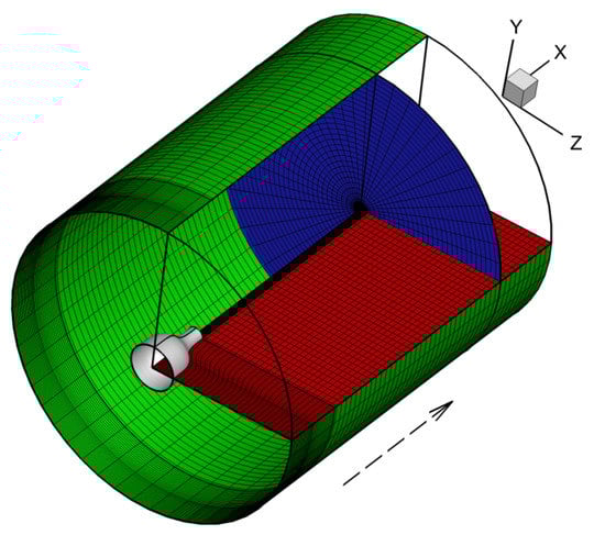
Figure 1.
Computational grid used for the LES. The nozzle is shown on the left using the gray surface. The azimuthal (red), axial (blue) and radial (green) surfaces are also marked to display the grid lines. Every tenth axial and radial point, and every other azimuthal point is marked on these surfaces. The dotted arrow indicate the jet-flow direction.
Further details of this mesh and additional resolution studies may be found in Goparaju and Gaitonde [54]. Stagnation conditions are provided at the nozzle inlet, and the remaining outer boundaries are treated using non-reflective characteristic boundary conditions. The singularity at the jet centerline can be effectively treated by assuming solution continuity [23]. The non-dimensional time-step-size used to ensure time-step-size independent results is . Results are presented by analyzing data over 110 characteristic time units, which was collected after the simulation achieved a statistically stationary state.
2.3. Validation
Although a detailed validation study may be found in Goparaju and Gaitonde [54], for completeness, we summarize some key results. As noted earlier, the underexpansion results in a series of expansion and compression cells in the jet plume. These are reflected in the centerline mean-streamwise velocity plotted in Figure 2a along with the corresponding experimental values. The experimental measurements provide values within an uncertainty limit of [55].
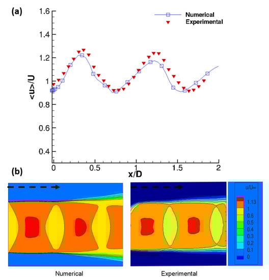
Figure 2.
(a) Comparison of mean-streamwise velocity along the centerline of the jet; (b) Comparison of shock cell structure on a vertical plane. Current computational results compared with corresponding experimental values. The experimental values plotted in (a) has an uncertainty of [55]. The horizontal dotted arrows indicate the flow direction in (b).
The agreement is clearly evident. Thus, the shock-cell strength and spacing are simulated in an accurate manner. A more comprehensive comparison is shown in Figure 2b, where simulations are plotted with PIV data. The spatial structure of the expansion and compression regions match each other, indicating that the numerical and experimental results are equivalent. Additional aspects of the validation may be found in Goparaju and Gaitonde [54].
2.4. Energy-Based Decomposition: Momentum Potential Theory
The analysis of underexpanded jets, relative to their perfectly expanded counterparts, is challenging for several reasons. In addition to the complex evolution of a fully turbulent shear layer, which by itself engenders various instabilities and acoustic emissions, the presence of viscous-inviscid interaction in the potential core results in additional modes of sound generation, and affects the formation and development of coherent structures. Prior efforts have provided significant insights into the sound characteristics of such jets (e.g., Tam [12]) as well as shock cell dynamics [56].
In the current work, we aim to further understand the physics of underexpanded jets from the perspective of energy transfer mechanisms. These mechanisms essentially convert various forms of fluctuation energy in the flow from one form to another, and thus provide a generalized framework to explain the observed features from a fundamental level. In this context, a suitable classification of fluctuation energy in a fluid medium is that based on Kovásznay’s approach [57]—i.e., hydrodynamic, acoustic and thermal. We refer to these three components as fluid-thermodynamic (FT) modes. They represent a very fundamental level of distinction in any fluid system, since they revert to the fluctuations in vorticity, pressure and entropy, respectively, in linear scenarios with a uniform base flow. In complex flows, such as underexpanded jets, the hydrodynamic mode naturally represents the curvature effects in shock-cell dynamics [58] and shear-layer vorticity. The acoustic mode can be used to track the origin and propagation of sound emissions. The thermal mode represents vorticity-entropy coupling, and becomes significant in heated jets.
Thus, the approach used here is predicated on an explicit decomposition of the turbulent fluctuations into the above three modes. Kovásznay’s approach is unsuited for this purpose, since it is difficult to adapt to a mean flow that is spatially varying. A powerful alternative is Doak’s MPT [28], which is employed here. The method provides a general technique to decompose a (carefully chosen, see below) fluctuating variable into the three FT modes, at all locations of the jet, including the nonlinear, turbulent region, as well as the relatively benign and linear (outer) nearfield/farfield.
MPT splits a judiciously chosen flow variable, the “momentum-density” or the mass-flux, , where is the density and is the velocity vector, into the three FT modes. It thus deviates from the Kovásznay approach, which establishes each mode with a different primitive variable. This choice circumvents the necessity of linearization, to define FT dynamics. The following discussion summarizes the salient features of MPT and aspects of its numerical implementation. Further details may be found in references [28,31,59,60].
2.4.1. Theoretical Considerations in MPT
MPT treats the momentum density vector, , as the primary field to be decomposed into the three FT components. The choice is motivated by the fact that the continuity equation is naturally linear in this variable. A generalized definition of FT modes is then adopted as follows. The hydrodynamic mode is the solenoidal component of . This ensures that vortical fluctuations in the flow are completely incorporated into the hydrodynamic component. The irrotational part of is further sub-divided into an isentropic and an isobaric component. The former is the acoustic mode, while the latter is the thermal mode. This generalized definition of FT modes makes it possible to uniquely define them in any continuum, time-stationary flow, even in the presence of discontinuities such as shocks, as will be shown for the first time in this study.
The splitting of momentum density is achieved through a Helmholtz decomposition:
here, is the mean solenoidal part, is the fluctuating solenoidal component and is the fluctuating scalar potential. For a statistically stationary flow, is assumed [28]. Equation (3), when substituted into the continuity equation, yields a Poisson equation for the scalar potential:
As discussed above, the acoustic () and thermal () components of the scalar potential are associated with isentropic and isobaric density-fluctuations, respectively. Therefore, . The individual scalar fields are then governed by the following Poisson equations:
p is the thermodynamic pressure, is the squared value of the instantaneous local speed of sound and S is the entropy defined as , evaluated with respect to the jet-exit conditions (subscript j).
MPT also provides a quantification of various modal energies and the corresponding source mechanisms inducing those fluctuations. This is encapsulated in Doak’s formulation of a transport equation for the fluctuating component of total enthalpy per unit mass [28], . This variable, denoted is composed of turbulent energy in the core of the jet, and gradually evolves into a purely acoustic form of energy in the near- and far-fields. The mean energy balance is expressed as:
is an “acceleration” vector defined as:
is the vorticity, is the entropy gradient and is the viscous stress tensor. The left hand side (LHS) of Equation (7) is the mean transport of by the three FT modes. The right hand side (RHS) of Equation (7) represents the source terms responsible for non-zero fluxes, again interpreted as the action of the three FT modes. Specifically, these source terms are the result of the FT modes interacting with an “acceleration” vector, , which is the combined effect of rotation, shear and entropy generation in the fluid. The last term on the RHS is dissipative in nature, and is associated to rate of change of entropy fluctuations.
The purpose of analyzing Equation (7) is to identify the most important source terms (RHS) of TFE, because they are responsible for the net energy flux that emanates out of the turbulent core. By interpreting the corresponding fields involved, specific physical mechanisms can be identified as crucial to intermittent generation of acoustic energy flux from the jet. It also identifies those regions in the jet, which contribute the most to these source mechanisms.
2.4.2. Numerical Implementation of MPT
The implementation of MPT-based analysis on the LES data involves two steps. The first is the decomposition of into its constituent FT modes, and the second step is calculating the TFE budget in Equation (7). The decomposition step is performed as follows:
- The mean solenoidal field, in Equation (3), is calculated as the average of instantaneous from the LES.
- The source term for the total scalar potential in Equation (4), , is obtained from the LES data, by obtaining the time-derivative of instantaneous density. This Poisson equation is then solved to obtain the total scalar potential, .
- The source term for the acoustic scalar potential in Equation (5), , is also calculated from the LES data, by obtaining the time-derivative of instantaneous pressure. Solution of this Poisson equation yields the acoustic scalar potential, .
- The thermal scalar potential is obtained using the relation, .
- Finally, the fluctuating solenoidal component is obtained as, .
The above calculations are performed for the full three-dimensional flowfield, using the generalized curvilinear form of the Poisson equation. A second order discretization yields a banded, highly sparse matrix, which is inverted using the BiCGSTAB [61] algorithm, parallelized using MPI framework. The boundary conditions are derived from the knowledge that at sufficient distance from the jet, fluctuations there are essentially acoustic. Likewise, all thermal and hydrodynamic fluctuations are damped out near the outer boundaries.
3. Results
To set the stage for discussion, we first provide in Figure 3 a general description of the underexpanded core and nearfield of the jet on an azimuthal slice containing the vertical plane.
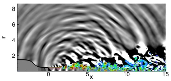
Figure 3.
Instantaneous snapshot of the jet. The expansion and compression regions in the potential core are highlighted using , in the region and . 10 equally spaced contour levels are used within the range 1 and . The shear layer is shown using magnitude of vorticity, using 11 contour levels between and 5, with blue and red representing the minimum and maximum levels, respectively. The acoustic emissions in the nearfield are visualized using divergence of velocity, using 10 contour levels between and . The jet-flow direction is from left to right.
The outline of the nozzle is marked with the black line. The color contours of vorticity magnitude highlight the developing shear layer, which, upon exiting the nozzle undergoes rapid destabilization at around diameters downstream of the nozzle exit. This results in the generation of large and small vortical roll-up regions, which eventually break down into a turbulent region. The potential core collapses at around 6 diameters downstream. The quantity, is employed in the core region around the axis to visualize the shock-expansion structure. For this, a domain defined by and is chosen to plot its contours, since this region encompasses the strongest compression and expansion cells. The mismatch of the nozzle exit pressure with the ambient results in the formation of a train of compression and expansion cells within the potential core of the jet. Lighter regions denote positive values of , i.e., the pressure increases along the direction of the velocity vector, thus indicating compression zones. Correspondingly, the darker or negative regions represent expansion zones, since here the flow experiences a negative (or favorable) pressure gradient along the flow direction. Finally, acoustic emissions from the jet are highlighted in the nearfield using the dilatation of the velocity vector. The dilatation can be viewed as a surrogate for acoustic pressure fluctuations [18]. Thus, in the nearfield, dilatation contours highlight regions of compression and expansion signifying propagating acoustic waves, due to the irrotational nature of the associated perturbations. In addition to coherent large-scale wavefronts emitted in the downstream direction, this underexpanded jet also produces significant wavefronts in the upstream and sideline directions, consistent with previous experiments [62] and computations [63]. Such a prominent upstream signature is usually absent in perfectly expanded jets, where the noise directivity of interest is along shallow angles.
3.1. Fluid-Thermodynamic Modal Features
We now present the characteristic features of the FT modes extracted from the underexpanded jet. Of the three components, the thermal field is omitted here for brevity, since it turns out to be of minor importance in this cold jet. For notational convenience, the cylindrical-coordinate vector components of the fluctuating hydrodynamic and acoustic modes will be denoted and , respectively. Furthermore, since the axial component is found to be the dominant one in both the hydrodynamic and acoustic fields, it is used for visualization.
Instantaneous snapshots of the hydrodynamic and acoustic modes are shown in Figure 4.
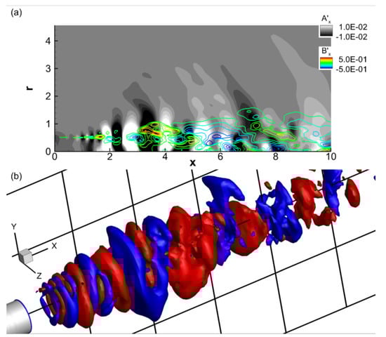
Figure 4.
(a) Instantaneous snapshot of the axial component of the hydrodynamic (contours) and acoustic (gray scale) modes; (b) Corresponding three-dimensional form of the acoustic wavepacket, shown using iso-levels of . The jet-flow direction in (b) is along the x-axis, as indicated by the axis-marker. The vertical lines in (b) are marked on the vertical plane and corresponds to and respectively, from left to right. The horizontal lines in (b) are marked on the vertical plane and corresponds to and respectively, from bottom to top.
Figure 4a shows axial components of the hydrodynamic and acoustic modes on the vertical azimuthal plane. The characteristic feature of the hydrodynamic mode (contours of Figure 4a) is its close representation of shear-layer vorticity and coherent structures displayed earlier in Figure 3. Localized zones of vortical instabilities appear at shock impingement locations along the edge of the nascent shear layer: the effect of shock cells on the modal dynamics will be quantified shortly. These shock-impingement locations act as sources of unsteadiness, perturbing the shear layer, unlike subsonic or perfectly expanded jets, where Kelvin-Helmholtz instabilities and their amplification is the main mechanism of shear-layer destabilization. The acoustic mode (gray scale in Figure 4a) displays a highly coherent wavepacket structure and is superficially similar to its corresponding form in a perfectly expanded jet [31]. The dominant downstream-traveling noise events are associated with the highly amplified lobes of this wavepacket. Thus, this analysis helps to establish a direct link between intermittent sound events in the nearfield with the dynamics in the core. As the contour legends of Figure 4a indicate, the acoustic response is at least an order of magnitude smaller than the hydrodynamic mode, which emphasizes the fact that a small fraction of turbulent energy is channeled into the highly destructive sound signature of the jet.
The origin of the acoustic wavepacket is closely linked to the irrotational fields developing around the initial vortical instabilities in the shear layer. A three-dimensional representation of the acoustic wavepacket is shown in Figure 4b using iso-levels of . The wavepacket clearly has coherence over a very large region relative to the hydrodynamic mode, and extends to around 7 jet diameters downstream. Higher azimuthal modes are limited to the nozzle-exit region, where the shear layer breaks down. The orderly core of the wavepacket between displays axisymmetric characteristics, with strong periodic fluctuations, which will be discussed in Section 3.4. Downstream of this zone, the wavepacket is primarily intermittent, with only the strongly amplified lobes surviving. Such intermittent events have been experimentally shown to contribute the most to the peak energy of shallow-angle mixing-noise in jets [64,65]. At further downstream locations beyond , the deceleration of the spreading shear layer reduces the mean Mach number (which is typically below ). In addition, the vorticity there is also minimal due to the milder gradients in the flow. Together, these effects weaken the irrotational response in the fluid, as well as the acoustic wavepacket.
The fluctuations induced by shock and expansion cells are now analyzed in terms of their FT components. For this purpose, the root-mean-squared (RMS) values of and are plotted along the centerline of the jet in Figure 5.
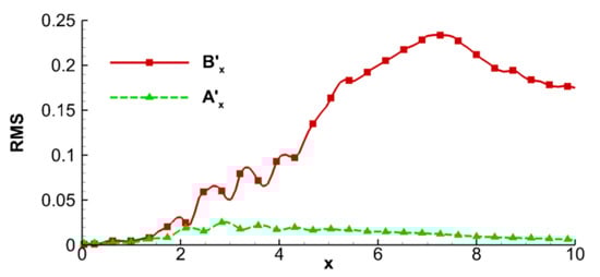
Figure 5.
RMS of the hydrodynamic and acoustic modes along the centerline of the jet.
No significant fluctuations are observed in the region upstream of , because the shear layer is thin and the two leading shock cells are relatively steady. The major fluctuations due to shock unsteadiness are observed between and , which induce the dominant peaks in the hydrodynamic signal within this axial extent. The corresponding fluctuations in the acoustic mode are relatively weak and the associated gradients are also significantly lower. The physical discontinuities associated with the shock cells are thus mainly confined to the hydrodynamic mode, and has minor impact on the acoustic mode. Beyond this axial range, the hydrodynamic mode amplifies due to the growing coherent structures and higher turbulence intensity. It peaks around , consistent with the trends observed in the vicinity of potential-core collapse (see e.g., Gaitonde and Samimy [23], Samimy et al. [66]). The much smaller acoustic mode exhibits peak values in the region of strong mean flow gradients, and is primarily bound within the potential core, consistent with the representation in Figure 4. Although not explicitly addressed here for brevity, this extent is essentially determined by the instability characteristics of the corresponding base flow.
3.2. Relationship of Nearfield Pressure and the Acoustic Mode
The fluctuating pressure is often scrutinized to characterize the physics of jets. In this section, we establish the relationship of the acoustic mode, with the pressure field, which is generally used as the acoustic variable in such studies [26,67,68].
For this purpose, Figure 6 displays an instantaneous snapshot of pressure perturbations on the vertical azimuthal slice in frame (a). The acoustic mode at the same instant is shown in frames (b), (c) and (d), using its axial, radial and azimuthal components, respectively. Note that the extracted acoustic mode, being a component of momentum density, is dimensionally different from pressure and is a vector quantity. The link between these two variables can be understood from Equation (5). A simple Fourier transform to wavenumber-frequency space shows that in a simplified one-dimensional scenario with a constant speed of sound, the acoustic spectrum is equivalent to the pressure spectrum scaled by the speed of sound. Such a simplification is not feasible in the multi-dimensional scenario of interest, and all components of the gradient of the acoustic-scalar-potential () must be considered, to account for various types of sound emission.
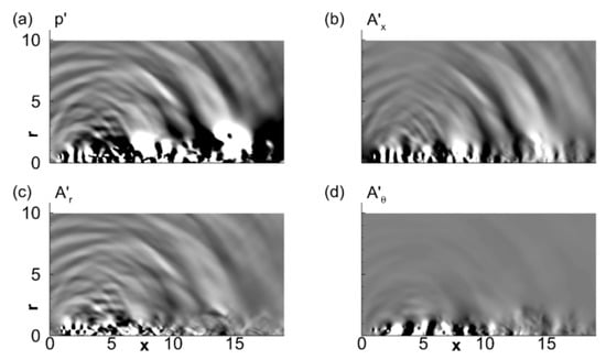
Figure 6.
Instantaneous snapshots of (a) pressure perturbations; (b) axial; (c) radial and (d) azimuthal components of the acoustic mode. The axial extent of the contours begin from the nozzle-exit station, and the jet-flow direction is from left to right. Frames a, b, c and d share the same abscissa and ordinate.
Figure 6 facilitates an understanding of the correspondence between the acoustic scalar potential and its gradient and the conventional pressure-based definition of the acoustic field. The pressure field in Figure 6a is reflective of several physical mechanisms at play in the turbulent jet. It includes signatures of initial shear-layer destabilization and roll-up, wavepackets in the potential core, structures with deteriorating coherence downstream of the potential core, large-scale lobes beyond 12 diameters (which are footprints of subsonically convecting hydrodynamic structures), intermittent acoustic wave-fronts in the downstream direction, upstream-propagating acoustic waves and finally, finer waves in the sideline direction. As discussed in prior works e.g., Tam et al. [10], Howe and Ffowcs [69], Lo et al. [70], these are contributors to various sound mechanisms in imperfectly expanded jets. The pressure signature of the jet is indicative of both hydrodynamic and acoustic phenomena. The irrotational-isentropic mode in Figure 6b–d is filtered of the hydrodynamic component, and is thus a clearer representation of the acoustically relevant dynamics within the jet. The axial component of the acoustic mode in frame (b) captures the wavepacket in the core of the jet, as well as the dominant downstream propagating intermittent waves, which contribute to the peak of the mixing noise spectrum. Low coherence [71] at the end of the potential core observed in pressure signals are removed from the acoustic field, which indicates that those incoherent fluctuations are fundamentally hydrodynamic in nature. The larger, convecting lobes in the downstream region are also absent in the acoustic mode. In addition to downstream sound radiation, the axial component of the acoustic mode also captures the upstream-propagating waves, which are typical in imperfectly expanded jets, and lead to feedback mechanisms resulting in screech generation [13]. The radial component of the acoustic mode in frame (c) primarily contributes to the sideline radiation, which includes fine-scale mixing noise [10] and broadband noise in imperfectly expanded jets [72]. The azimuthal component in frame (d) has minor contribution outside the shear layer, underlining the azimuthally coherent nature of acoustic radiation from circular jets. The wavepacket form is characteristic of the axial component of the acoustic mode, which thus naturally becomes the crucial field for acoustic predictive and modeling purposes. It is evident that, the pressure contains both acoustic and hydrodynamic signatures, while taken together, the three components of the irrotational-isentropic mode fully represent all the acoustic (but not hydrodynamic) features of interest in the turbulent and nearfield regions.
A quantitative comparison of the above equivalence is now provided in Figure 7. For this, the time accurate pressure and acoustic perturbations are recorded along a horizontal array at a radius, at various axial locations. The power spectral density (PSD) of both signals are then computed and compared using combined PSD of axial and radial components of the acoustic mode. The location of each point is marked in each frame of Figure 7. The first location, at , is upstream of the nozzle-exit station and has contribution from the upstream propagating wavefronts, and displays a relatively narrow peak around . Further downstream, at and , the nearfield signature of the jet is dominated by fine-scale waves, seen in Figure 6. The spectrum progressively attains a broadband nature, characteristic of omni-directional sideline radiation in jets. At locations and beyond, the nearfield spectrum begins to display a prominent peak at a low , typically , where peak noise directivity is observed. This is attributed to the coherent wavefronts emitted intermittently along the shallow angle direction. In this specific jet, peak sound directivity is observed at , which is identified as its column mode frequency. At all locations considered, the combined PSD of the acoustic mode fully recreates the information in pressure, (which is naturally filtered to contain mostly acoustic information at this radial location). Thus, further discussions involving near- and far-field acoustic data will consider the FT-decomposed acoustic mode of the jet.
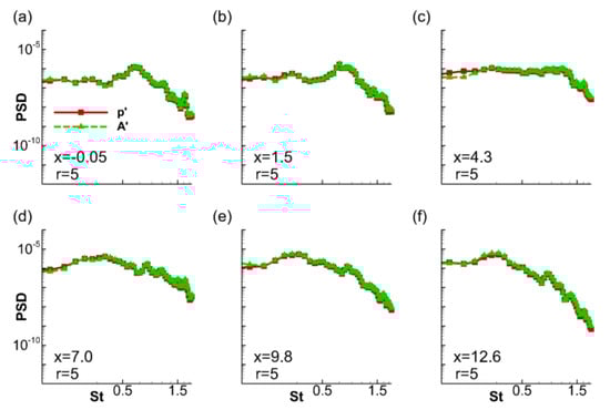
Figure 7.
Comparison of PSDs obtained from pressure fluctuations and the acoustic mode at various locations in the computational nearfield, as indicated in each frame. Frames a-f share the same abscissa and ordinate.
3.3. Shock-Cell Dynamics and Their Acoustic Imprint
A distinguishing feature of underexpanded jets is the presence of shock and expansion cells in the core-flow region, and its associated sound signature.To characterize the nearfield acoustic properties, including the effects of the shock cells, a spectral analysis of the acoustic mode is presented in Figure 8.
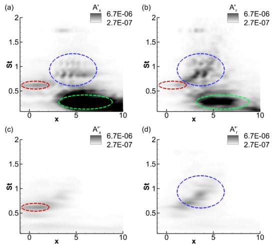
Figure 8.
Spectral variation of acoustic signature along the axial direction, at . The contours represent PSD of (a) ; (b) ; (c) upstream propagating components in and (d) upstream propagating components in .
Specific acoustic signals are obtained at a radius, , along various axial locations. The PSD of the signal as a function of is plotted at the corresponding axial location, resulting in a contour plot. The axial component of the acoustic mode, at , subjected to this spectral analysis, is shown in Figure 8a, where the PSD contours are plotted using the axial location of the probe along the horizontal axis and frequency along the vertical axis. Figure 8b is the corresponding result for the radial component of the acoustic mode, . Figure 8c,d represent the same results for and , respectively, but by retaining only the upstream propagating waves i.e., with negative phase velocities.
In Figure 8a, depending on the spectral and axial ranges, three separate zones are marked using dotted curves, which represent various components of acoustic radiation from this jet. The most prominent among these three is the one encompassed by the green oval in the range and . This is the mixing noise due to coherent structures, emitted as well-defined, shallow-angle wavefronts in the downstream direction, and is observed in both perfectly and imperfectly expanded jets. The other two components are features specific to imperfectly expanded jets, due to the interaction of the shock-cells and the developing shear layer. The region marked with the red oval ( and ) represents a localized spectral support around a peak frequency, . The axial extent of this component indicates that it is limited to the upstream region of the nozzle. This component is the one that mostly retains its spectral support in Figure 8c also, which implies that it constitutes upstream traveling waves. Experimental results of similar jet-configurations [16,73] identify narrowband component at as a screech tone, formed as a result of the feedback mechanism between the vortex-shock-cell interaction and the resulting upstream propagating waves actuating instabilities at the nozzle exit. The third region, marked with the blue curve, and , displays vertical patterns with intermittent horizontal peaks at and . Similar vertical stripes were also observed in the pressure signal obtained in the core of a computed underexpanded jet in Arroyo et al. [68]. These patterns are associated with the axial locations of peak compression in the oscillating shock train. Such wave-train oscillations also impart a corresponding signature to the acoustic nearfield. Since these are primarily one-dimensional oscillations in the streamwise direction, their signature is well-preserved in the streamwise acoustic component, , even in the nearfield.
The spectral analysis of the radial component of the acoustic mode, in Figure 8b also identifies three separate regions in the nearfield. The first two components, namely turbulent mixing noise and screech, are relatively less prominent in this component, because these are mostly axial transport mechanisms in the acoustic wave. On the other hand, the third component, marked with the green curve, has a qualitatively different spatial support compared to the corresponding results of . It displays an elongated lobe-like structure, similar to the “banana-shaped” pattern discussed in Arroyo et al. [68], Savarese et al. [74]. This is characteristic of broadband shock associated noise (BBSAN), and its shape is associated to Doppler effect of shock cell noise [75]. The peak frequency around which this component occurs can be seen to increase towards lower angles in the downstream direction. There is also a signature of the strongest tone of the third component (blue curve) of , at in also. The low contour values in the upstream components of in Figure 8d imply that, the most energetic waves in BBSAN is predominantly downstream-propagating. It also highlights the contribution of the upstream-propagating waves to the “banana-shaped” pattern associated with BBSAN.
Additional insights into shock-cell dynamics are obtained by applying proper orthogonal decomposition (POD) to the shock field, defined using . When applied to a spatio-temporal dataset, , POD realizes a separation of spatial and temporal dependencies, representing the data in the form:
N is the total number of snapshots, which determines the total number of POD modes, is the temporal variation of the POD mode, and is its corresponding spatial support. In the method of snapshots [76,77] adopted here, the temporal coefficients are obtained as the eigenvectors of the spatial correlation matrix, , which is defined as:
The inner product in the cylindrical coordinate system used here is defined as:
The spatial modes, , are the projection of the data snapshots onto the temporal coefficients:
is the eigenvalue corresponding to the eigenvector of the spatial correlation matrix, , and is indicative of the energy contained in the corresponding POD mode, . Thus, POD extracts a mutually orthogonal basis for the data, which is optimal in terms of energy content.
The leading POD modes, Figure 9, with most of the energy naturally yield the peak fluctuations in : these correspond to the locations of strongest oscillations in the compression and expansion regions. Each frame of Figure 9 contains the spatial support of a given POD mode, and the PSD of its time coefficient, . Since POD modes may contain multiple frequencies, the PSD provides additional clarity in terms of the spectral content in each POD mode. Due to the highly oscillatory nature of the shock cells, the leading POD modes arise in pairs, which were identified through similarities in their respective time-coefficient-spectra. Hence, the results presented here include only one of each pair. Specifically, the first, third, fifth and seventh modes are shown in Figure 9a–d, respectively. The most energetic oscillations are observed in the third-to-sixth shock cells, with the corresponding modal shape in frame (a). Its PSD indicates a relatively broadband nature between . The location of this axial region between is directly beneath the peaks observed in the shock-associated noise components in Figure 8a,b, which identifies this shock-unsteadiness as a prime contributor to the nearfield acoustic signature in the sideline direction. This is also consistent with the idea of Norum and Seiner [78], who associated BBSAN with the relatively weaker, but more dynamic shock cells at downstream locations, i.e., those following the initial relatively steady strong compression or expansion waves. The higher POD modes in Figure 9b,c progressively show increased spectral support at a higher frequency of , the signature of which is also observed in the nearfield acoustic signals (Figure 8a,b). This higher-frequency component of shock unsteadiness is primarily limited to the thin shear layer, unlike the lower broadband content, which is observed throughout the radial extent of the potential core. The seventh POD mode in Figure 9d also identifies prominent fluctuations in the fourth, fifth and sixth shock cells, with peak frequency around .
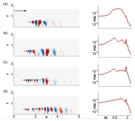
Figure 9.
POD modes of the field , along with the PSD of the corresponding modal time-coefficient. The modes shown are: (a) mode 1; (b) mode 3; (c) mode 5 and (d) mode 7. The horizontal dotted arrow in (a) marks the jet-flow direction. Frames a-d share the same abscissa and ordinate.
3.4. Predictive Advantages of the Acoustic Mode
The explicit extraction and quantification of the hydrodynamic and acoustic fluctuations in the jet has advantages not only in deriving a better understanding of the flow, but also in prediction techniques. The acoustic mode can be viewed as a response of the compressible flow to hydrodynamic instabilities developing in the shear layer. The MPT-based filtering accurately isolates that fraction of energy which eventually becomes the radiated sound field. In addition to the acoustic mode actuated in the initial developmental region of the shear layer, coherent and small-scale eddies often constitute additional sources for the acoustic mode within the turbulent region of the jet. The acoustic mode follows an evolution equation as described in Doak [28] with continuous inputs from the source terms generated due to turbulence. This is also evident from Equation (7), where any non-zero source term on the RHS will lead to a net production of FT fluxes from within a control volume in the fluid. A natural application of the MPT-based energy analysis is to efficiently extract the acoustic energy in the turbulent region to understand its sources and for sound prediction and modeling. For a perfectly expanded jet, the utility of such an exercise may be found in Unnikrishnan and Gaitonde [31].
We now explore the use of the decomposition to efficiently predict the qualitative and quantitative features of the radiated energy, even under non-ideal operating conditions. The evolution equation for the scalar potential defining the irrotational field, discussed in Doak [28], contains non-zero source terms from hydrodynamic and entropic fluctuations. The effects of these sources are reflected in the MPT-extracted acoustic mode from the LES, which includes all nonlinearities and non-homogeneous source mechanisms associated with turbulence. For simplicity, the analysis below neglects the thermal component of the energy, since it is essentially dormant for this field. It is also assumed that the region outside this LES solution is an inviscid, irrotational and linear domain, which simplifies the momentum equation (originally written in terms of FT modes) to:
Taking the gradient of Equation (5) (which is essentially the continuity equation for the irrotational field) and using the above relation, we obtain the equation:
This is in effect the homogeneous wave propagator equation for the gradient of acoustic scalar potential, which implies that each component of the acoustic vector field defined as , is propagated according to a simple wave equation, outside the acoustic source region. Although this feature is also true for the pressure variable, the region of validity of these simplifying assumptions is much further away from the core of the jet, due to the hydrodynamic effects captured by the pressure fluctuations. The acoustic mode, due to its filtered properties, allows one to use a propagating surface as close as diameters from the jet axis, as will be shown shortly. In addition to this aspect, the choice of the acoustic mode for prediction is also observed to provide relatively quickly-converging statistics, which is useful in shortening the LES time-series used for prediction. This is because, the hydrodynamic component engenders more turbulent behavior, resulting in a poorer reduced order behavior, compared to the acoustic mode.
Before discussing the prediction results, we first analyze the dominant source mechanisms which contribute to the net energy flux from the jet, as encapsulated in the TFE equation, Equation (7). The results are shown in Figure 10. The underlying idea is to demarcate a suitable zone for the homogeneous wave propagator as close as possible to the jet centerline, based on the distribution of these source terms. For a succinct discussion, we choose to identify regions of prominent mean source activity, attributed to the three FT modes. These include the terms, , , and , which are the mean TFE source terms due to the hydrodynamic, acoustic and thermal fluctuations, respectively, in the jet. These are named HS, AS and TS, respectively and plotted on an azimuthal slice in Figure 10a–c, respectively. Consistent with the observations in a perfectly expanded supersonic jet [31], the hydrodynamic source (HS) is the primary production mechanism of TFE. Large contributions are evident in the developing shear layer (), with peak values in the inner half of the shear layer. A narrow sink zone is also observed along the edge of the potential core, where TFE is dissipated through entrainment mechanisms [31]. The acoustic source, AS, in Figure 10b also has predominantly positive nature, implying TFE production, but is not a significant contributor to the source mechanism, compared to the hydrodynamic mode. The thermal source (TS) in Figure 10c displays sink characteristics in the inner half of the shear layer but acts as a weak source of TFE in the outer region. A quantitative comparison of the three source mechanisms is also provided in Figure 10d, by plotting these source terms extracted along a vertical line at (as marked in frames (a), (b) and (c)). As discussed above, the hydrodynamic source dominates over the other terms, with peak amplitude in the vicinity of the lipline of the jet. This analysis thus establishes the compact radial support of the TFE source mechanisms, suggesting that the acoustic mode is primarily propagated as a homogeneous wave beyond .
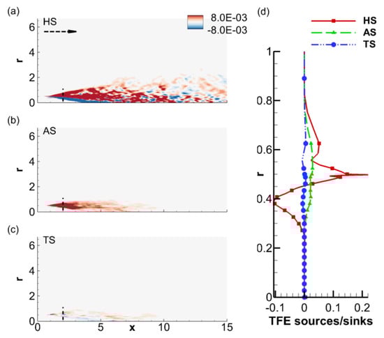
Figure 10.
Mean (a) hydrodynamic; (b) acoustic and (c) thermal sources of TFE; (d) Radial profile of the three source terms along the dotted vertical line at , shown in (a). The horizontal dotted arrow in (a) marks the mean-flow direction of the jet. Frames a, b, and c share the same abscissa and ordinate.
We now show the prediction capability of the acoustic mode based on information collected at , which is much closer to the axis than that employed with typical Ffowcs Williams-Hawkings approaches. The comparison of the LES solution with the wave propagator prediction is shown in Figure 11 using an instantaneous snapshot of , obtained from the respective calculations. The result from LES is presented in Figure 11a. The contours of are demarcated into two regions, separated by a horizontal dotted line at . The contours below have a prominent wavepacket form, as discussed earlier in the context of Figure 4. It also shows intermittent amplified lobes downstream at lower frequencies, which engenders the radiated large-scale acoustic waves. The acoustic wavepacket in this region continuously receives inputs (sources) from the turbulent fluctuations, and also undergoes non-linear interactions with itself (e.g., lobe merging and frequency shifts), resulting in a relatively complex dynamics, which is discussed further below. Conversely, outside this region, , due to the absence of significant source terms, the evolution of the acoustic wavepacket essentially reduces to a benign wave propagation problem. To obtain the acoustic predictions, the homogeneous wave propagator equation, with ambient speed of sound, is forced with time-accurate values of at in the region , and propagated to the farfield, to a distance of 75 diameters. An excellent match is observed between the LES and wave propagator (WPr) results, with all the dominant intermittent wavefronts in the downstream direction being captured accurately. The upstream components as well as the fine-scale waves in the sideline direction are also well predicted.
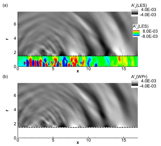
Figure 11.
(a) An instantaneous acoustic field, , extracted from the LES; (b) The predicted field at the corresponding time-instant, using a homogeneous wave propagator. The wave propagator is forced at (marked using a horizontal dotted line). The color and gray-scale contours in (a) simply demarcate the zone of prediction in the wave propagator solution for easy comparison. The jet-flow direction is from left to right.
The above analysis justifies the use of the predicted acoustic mode to calculate farfield directivity and sound pressure levels (SPL). The farfield SPL is obtained along an arc of 75 diameters on the vertical azimuthal slice and plotted in polar coordinates (relative to the jet axis) for different . The results, provided in Figure 12, show that the spectral shape is generally in good agreement with the farfield directivity shown for similar jets [16,73]. The peak SPL is observed at a shallow angle of 30, as expected, and has a value of ∼88 dB. Differences from the experimental observation of approximately 4 dB are attributable to the laminar jet exit conditions employed here. Compared to an initially-turbulent jet, the breakdown of an initially-laminar shear layer results in larger coherent structures, and thus induces stronger lobes in the acoustic wavepacket, contributing to shallow-angle noise.
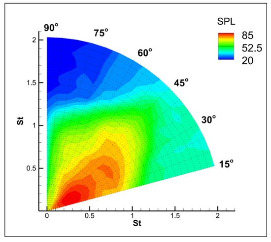
Figure 12.
Farfield sound pressure levels along a polar arc at 75 diameters.
In order to succinctly represent the dominant dynamics of the acoustic wavepacket, we analyze its temporal evolution on the vertical azimuthal plane using POD. The first six modes are plotted in Figure 13.
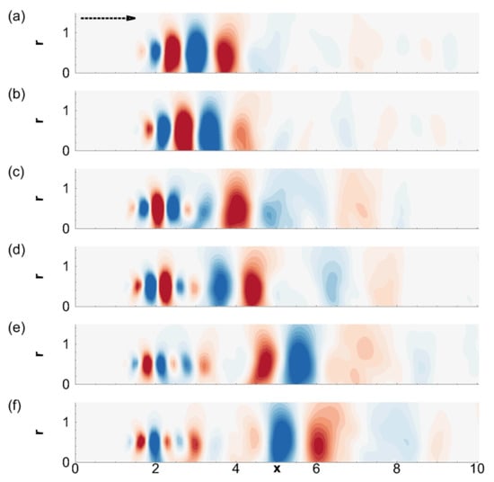
Figure 13.
POD modes of the acoustic field, . The modes shown are: (a) mode 1; (b) mode 2; (c) mode 3; (d) mode 4; (e) mode 5 and (f) mode 6. The horizontal dotted arrow in (a) marks the jet-flow direction. Frames a-f share the same abscissa and ordinate.
Although not shown here, the frequency spectra of modes 1 and 2, modes 3 and 4 and modes 5 and 6 are similar, indicating that they are mode-pairs. The spectra of the acoustic POD modes exhibit a relatively narrowband nature in their frequency content compared to those in the shock field (Figure 9). This suggests a more orderly form of acoustic response, compared to the chaotic hydrodynamic turbulent fluctuations. The first two POD modes of the acoustic wavepacket in Figure 13a,b have a peak frequency of , and constitute its main body. From a modeling perspective, this is the basic or principal [79] frequency of the radiating wavepacket. It exists within the main body of the potential core, and is highly periodic. Naturally, it also represents the most energetic component of acoustic fluctuations and appears as the first two POD modes. The second pair in Figure 13c,d exhibits an interesting scenario: its spectra have two peaks: a major peak at and a minor peak at . The former lower frequency corresponds to the larger lobes observed in the zone and the latter, higher frequency is representative of the smaller lobes in the initial transition stage of the shear layer, mostly dominated by Kelvin-Helmholtz waves. These two components are also visible in the third pair of POD modes in Figure 13e,f, but here, the lower frequency lobes at , observed beyond , are relatively more prominent. These lobes are intermittently generated from the periodic principal content of the wavepacket (Figure 13a,b) due to nonlinear interactions, such as merging or coalescing, vortex pairing or intrusion events. The intermittent lobes amplified in the course of these events directly contribute to the coherent sound waves emitted along shallow angles. This can also be understood from the fact that the peak frequency of the downstream lobes of the acoustic wavepacket matches the frequency of peak SPL along the 30 angle to the jet axis (which is also as seen in Figure 12).
The above analysis further aids in associating various energy mechanisms in the core that are significant to the farfield sound of the jet. This is achieved by correlating the time-evolution of the POD modes of a suitably chosen field with the farfield sound signature of the jet, e.g., Magstadt et al. [16]. Here we choose the POD modes of the acoustic wavepacket, since it incorporates all the information of the radiated sound field. The time-coefficients of the first 12 POD modes of the acoustic wavepacket are correlated with the farfield acoustic signature of the jet, at various polar angles. The maximum cross-correlation coefficients are plotted in polar coordinates in Figure 14.
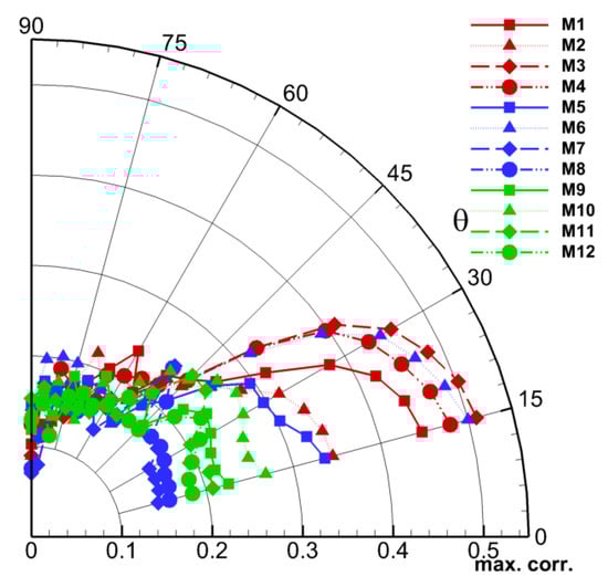
Figure 14.
Maximum cross-correlation values between the time coefficients of the first 12 POD modes of the acoustic wavepacket, and the farfield acoustic signal rerecorded at various polar angles at a distance of 75 jet diameters.
The radial coordinate represents the maximum-correlation value, and the angular coordinate is the polar angle at a radius of 75 diameters, where the correlation is calculated. The legend “M#” is the POD-mode-number used to calculate the correlation. It is evident that the first six POD modes are highly correlated to farfield noise, with peak values generally above , for shallow angles below 45. These values are significantly greater than those experimentally observed [16] at shallow angles, when POD modes of velocity were used for the correlation. The MPT-extracted acoustic mode thus improves the farfield acoustic correlations by filtering out the energetic, but non-radiated hydrodynamic events in the velocity signal. Peak correlations are observed at shallow angles for POD modes 3, 4 and 6. As explained above, these POD modes are representative of the intermittent lobes at downstream locations of the acoustic wavepacket, that radiate as coherent waves (Figure 13). As expected, the peak correlation reduces towards sideline direction, due to the fine-scale, omni-directional nature of sound waves in that region [32]. Thus, the dynamics of a few leading POD modes of the acoustic wavepacket can yield significant insights into the nature of peak acoustic directivity of the jet, even in underexpanded conditions.
4. Conclusions
An underexpanded jet is considered with the aim of understanding the physical mechanisms underlying turbulent shear-layer interactions with compression and expansion cells in the jet plume, and its associated acoustic ramifications. An energy-based approach is employed to identify vortical and acoustic fluctuations in the nonlinear and linear regions of the flowfield. The energy-based approach follows the theoretical development of Doak’s momentum potential theory (MPT), which splits momentum-density fluctuations in the underexpanded jet into its hydrodynamic, acoustic and thermal components. These can be considered as the three fundamental types of fluid fluctuations, in a Kovásznay-type framework.
The hydrodynamic mode is defined as the solenoidal part of momentum fluctuations, and the acoustic mode is its irrotational and isentropic component. It is shown that this decomposition can be successfully implemented even in the presence of physical discontinuities in the plume. While the hydrodynamic mode captures the shear-layer vortices and shock-fluctuations in the core, the acoustic mode has a spatio-temporally coherent wavepacket form, and yields the acoustic signature in the nearfield, usually characterized through pressure fluctuations. The acoustic mode also retains the imprint of shock fluctuations in the form of vertical spectral strips, in the range, and , and has energy peaks at and . The “banana-shaped” lobe corresponding to broadband shock associated noise (BBSAN) discussed in literature is also identified in the nearfield. A localized peak is observed at , mainly constituted by upstream propagating waves, which bears close similarity to the screech frequency identified in the corresponding experimental configuration. These sound signatures are then assessed from the perspective of shock-cell dynamics, by extracting the leading orthogonal modes of the shock field. The third-to-sixth shock cells displaying the most energetic oscillations are found to directly contribute to the shock associated acoustic signature.
The source terms that result in inter-modal energy transfers are evaluated. The inner half of the shear layer is found to have the peak source terms that contribute to these transfer mechanisms. Additionally, the compact radial support of the source terms provides an opportunity to use the acoustic mode with a simple homogeneous wave propagation technique to predict farfield noise of the jet. The recreated near- and far-field sound pressure levels show peak noise directivity at 30 from the axis, at . The POD analysis of the acoustic wavepacket used for propagation reveals two prominent dynamics. The first is the highly periodic internal frequency of the wavepacket at , which defines its spatio-temporally modulated wave-train and envelope. The second major component is comprised of the relatively intermittent lobes at a lower frequency of , which appear downstream of the potential core as a result of the nonlinear evolution of the internal frequency. This component correlates well with the farfield sound signal of the jet, and has the same frequency as the peak farfield sound spectra. Thus, the POD analysis of the acoustic mode identifies the reduced-order-mode that is most efficient in defining the farfield sound spectra of the jet.
Author Contributions
U.S.N. performed the decomposition and detailed modal analysis, and wrote the first draft of the manuscript; The source data was generated using Large-Eddy Simulations by D.G. and K.G.; K.G. performed the validation study; All further drafts were modified by U.S.N. and D.G., with inputs from K.G.; All authors had full access to all of the data.
Acknowledgments
This research was supported by the Office of Naval Research (Grants: N00014-17-1-2584) monitored by S. Martens. The simulations were performed with a grant of computer time from the DoD HPCMP DSRCs at AFRL, NAVO and ERDC, and the Ohio Supercomputer Center.
Conflicts of Interest
The authors declare no conflict of interest. The founding sponsors had no role in the design of the study; in the collection, analyses, or interpretation of data; in the writing of the manuscript, and in the decision to publish the results.
References
- Suzuki, T. Wave-Packet Representation of Shock-Cell Noise for a Single Round Jet. AIAA J. 2016, 54, 3903–3917. [Google Scholar] [CrossRef]
- Panda, J.; Seasholtz, R.G. Measurement of shock structure and shock–vortex interaction in underexpanded jets using Rayleigh scattering. Phys. Fluids 1999, 11, 3761–3777. [Google Scholar] [CrossRef]
- Owston, R.; Magi, V.; Abraham, J. Fuel-Air Mixing Characteristics of DI Hydrogen Jets. SAE Int. J. Eng. 2009, 1, 693–712. [Google Scholar] [CrossRef]
- Adamson, T.C.; Nicholls, J.A. On the structure of jets from highly underexpanded nozzles into still air. J. Aerosp. Sci. 1959, 26, 16–24. [Google Scholar] [CrossRef]
- Bonelli, F.; Viggiano, A.; Magi, V. A numerical analysis of hydrogen underexpanded jets under real gas assumption. J. Fluids Eng. 2013, 135, 121101. [Google Scholar] [CrossRef]
- Avital, G.; Cohen, Y.; Gamss, L.; Kanelbaum, Y.; Macales, J.; Trieman, B.; Yaniv, S.; Lev, M.; Stricker, J.; Sternlieb, A. Experimental and computational study of infrared emission from underexpanded rocket exhaust plumes. J. Thermophys. Heat Transf. 2001, 15, 377–383. [Google Scholar] [CrossRef]
- Norum, T.D.; Seiner, J.M. Measurements of Mean Static Pressure and Far Field Acoustics of Shock Containing Supersonic Jets; NASA Technical Report; NASA Langley Research Center: Hampton, VA, USA, September 1982.
- André, B.; Castelain, T.; Bailly, C. Experimental exploration of underexpanded supersonic jets. Shock Waves 2014, 24, 21–32. [Google Scholar] [CrossRef]
- Raman, G. Supersonic jet screech: Half-century from Powell to the present. J Sound Vib. 1999, 225, 543–571. [Google Scholar] [CrossRef]
- Tam, C.K.W.; Viswanathan, K.; Ahuja, K.K.; Panda, J. The sources of jet noise: Experimental evidence. J. Fluid Mech. 2008, 615, 253–292. [Google Scholar] [CrossRef]
- Tam, C.K.W. Jet noise generated by large-scale coherent motion. In Aeroacoustics of Flight Vehicles: Theory and Practice. Volume 1: Noise Sources; NASA Langley Research Center, Aeroacoustics of Flight Vehicles: Hampton, VA, USA, 1991; Volume 1. [Google Scholar]
- Tam, C.K.W. Supersonic jet noise. Ann. Rev. Fluid Mech. 1995, 27, 17–43. [Google Scholar] [CrossRef]
- Powell, A. On the mechanism of choked jet noise. Proc. Phys. Soc. Sect. B 1953, 66, 1039. [Google Scholar] [CrossRef]
- Harper-Bourne, M. The noise from shock waves in supersonic jets. AGARD-CP-131 1973, 11, 1–13. [Google Scholar]
- Tam, C.K.W.; Tanna, H.K. Shock associated noise of supersonic jets from convergent-divergent nozzles. J. Sound Vib. 1982, 81, 337–358. [Google Scholar] [CrossRef]
- Magstadt, A.S.; Berry, M.G.; Berger, Z.P.; Shea, P.R.; Ruscher, C.J.; Gogineni, S.P.; Glauser, M.N. Flow Structures Associated with Turbulent Mixing Noise and Screech Tones in Axisymmetric Jets. Flow Turbul. Combust. 2017, 98, 725–750. [Google Scholar] [CrossRef]
- Freund, J.B. Noise sources in a low-Reynolds-number turbulent jet at Mach 0.9. J. Fluid Mech. 2001, 438, 277–305. [Google Scholar] [CrossRef]
- Freund, J.B.; Lele, S.K.; Moin, P. Numerical simulation of a Mach 1.92 turbulent jet and its sound field. AIAA J. 2000, 38, 2023–2031. [Google Scholar] [CrossRef]
- Bogey, C.; Bailly, C. Computation of a high Reynolds number jet and its radiated noise using large eddy simulation based on explicit filtering. Comput. fluids 2006, 35, 1344–1358. [Google Scholar] [CrossRef]
- Schulze, J.; Sesterhenn, J. Numerical simulation of supersonic jet-noise. Proc. Appl. Math. Mech. 2008, 8, 10703–10704. [Google Scholar] [CrossRef]
- Bodony, D.J.; Lele, S.K. On using large-eddy simulation for the prediction of noise from cold and heated turbulent jets. Phys. Fluids 2005, 17, 085103. [Google Scholar] [CrossRef]
- Bonelli, F.; Viggiano, A.; Magi, V. How does a high density ratio affect the near-and intermediate-field of high-Re hydrogen jets? Int. J. Hydrogen Energy 2016, 41, 15007–15025. [Google Scholar] [CrossRef]
- Gaitonde, D.V.; Samimy, M. Coherent structures in plasma-actuator controlled supersonic jets: Axisymmetric and mixed azimuthal modes. Phys. Fluids 2011, 23, 095104. [Google Scholar] [CrossRef]
- Nichols, J.; Ham, F.; Lele, S.; Bridges, J. Aeroacoustics of a supersonic rectangular jet: Experiments and LES predictions. In Proceedings of the 50th AIAA Aerospace Sciences Meeting including the New Horizons Forum and Aerospace Exposition, Nashville, Tennessee, 9–12 January 2012. [Google Scholar]
- Li, X.; Zhou, R.; Yao, W.; Fan, X. Flow characteristic of highly underexpanded jets from various nozzle geometries. Appl. Therm. Eng. 2017, 125, 240–253. [Google Scholar] [CrossRef]
- Morris, P.J.; Miller, S.A.E. Prediction of broadband shock-associated noise using Reynolds-averaged Navier-Stokes computational fluid dynamics. AIAA J. 2010, 48, 2931–2944. [Google Scholar] [CrossRef]
- Suzuki, T.; Lele, S.K. Shock leakage through an unsteady vortex-laden mixing layer: Application to jet screech. J. Fluid Mech. 2003, 490, 139–167. [Google Scholar] [CrossRef]
- Doak, P.E. Momentum potential theory of energy flux carried by momentum fluctuations. J. Sound Vib. 1989, 131, 67–90. [Google Scholar] [CrossRef]
- Goldstein, M.E. On Identifying the Sound Sources in a Turbulent Flow; NASA Technical Report; NASA Glenn Research Center: Cleveland, OH, USA, 2008.
- Jordan, P.; Daviller, G.; Comte, P. Doak’s momentum potential theory of energy flux used to study a solenoidal wavepacket. J. Sound Vib. 2013, 332, 3924–3936. [Google Scholar] [CrossRef]
- Unnikrishnan, S.; Gaitonde, D.V. Acoustic, hydrodynamic and thermal modes in a supersonic cold jet. J. Fluid Mech. 2016, 800, 387–432. [Google Scholar] [CrossRef]
- Bogey, C.; Bailly, C. An analysis of the correlations between the turbulent flow and the sound pressure fields of subsonic jets. J. Fluid Mech. 2007, 583, 71–97. [Google Scholar] [CrossRef]
- Panda, J.; Seasholtz, R.G. Experimental investigation of density fluctuations in high-speed jets and correlation with generated noise. J. Fluid Mech. 2002, 450, 97–130. [Google Scholar] [CrossRef]
- Arroyo, C.P.; Daviller, G.; Puigt, G.; Airiau, C. Shock-cell noise of supersonic under expanded jets. In Proceedings of the 50th 3AF International Conference on Applied Aerodynamics, Toulouse, France, 29 March–1 April 2015. [Google Scholar]
- Sinayoko, S.; Agarwal, A.; Sandberg, R.D. On wavenumber spectra for sound within subsonic jets. arXiv, 2013; arXiv:1311.5358. [Google Scholar]
- Grizzi, S.; Camussi, R.; Di Marco, A. Experimental Investigation of pressure fluctuations in the near field of subsonic jets at different Mach and Reynolds numbers. In Proceedings of the 18th AIAA/CEAS Aeroacoustics Conference, Colorado Springs, CO, USA, 4–6 June 2012. [Google Scholar]
- Krothapalli, A.; Hsia, Y.; Baganoff, D.; Karamcheti, K. The role of screech tones in mixing of an underexpanded rectangular jet. J. Sound Vib. 1986, 106, 119–143. [Google Scholar] [CrossRef]
- Tam, C.K.W. Stochastic model theory of broadband shock associated noise from supersonic jets. J. Sound Vib. 1987, 116, 265–302. [Google Scholar] [CrossRef]
- Lumley, J.L. The structure of inhomogeneous turbulent flows. In Atmospheric Turbulence and Radio Wave Propagation; House Nauka: Moscow, USSR, 1967; pp. 166–178. [Google Scholar]
- Lighthill, M.J. On Sound Generated Aerodynamically: I. General Theory. Proc. R. Soc. Lond. A 1952, 211, 564–587. [Google Scholar] [CrossRef]
- Lighthill, M.J. On Sound Generated Aerodynamically: II. Turbulence as a Source of Sound. Proc. R. Soc. Lond. A 1954, 222, 1–32. [Google Scholar] [CrossRef]
- Ffowcs Williams, J.E. The noise from turbulence convected at high speed. Philos. Trans. R. Soc. Lond. A 1963, 255, 469–503. [Google Scholar] [CrossRef]
- Shea, P.R.; Berger, Z.P.; Berry, M.G.; Glauser, M.N.; Gogineni, S. Low-dimensional modeling of a Mach 0.6 axisymmetric jet. In Proceedings of the 52nd Aerospace Sciences Meeting, National Harbor, MA, USA, 13–17 January 2014. [Google Scholar]
- Gaitonde, D.V. Analysis of the near field in a plasma-actuator-controlled supersonic jet. J. Propuls. Power 2012, 28, 281–292. [Google Scholar] [CrossRef]
- Speth, R.L.; Gaitonde, D.V. Parametric Study of a Mach 1.3 Cold Jet Excited by the Flapping Mode Using Plasma Actuators. Comput. Fluids 2013, 84, 16–34. [Google Scholar] [CrossRef]
- González, D.R.; Speth, R.L.; Gaitonde, D.V.; Lewis, M.J. Finite-time Lyapunov exponent-based analysis for compressible flows. Chaos Int. J. Nonlinear Sci. 2016, 26, 083112. [Google Scholar] [CrossRef] [PubMed]
- Steger, J.L. Implicit finite-difference simulation of flow about arbitrary two-dimensional geometries. AiAA J. 1978, 16, 679–686. [Google Scholar] [CrossRef]
- Vinokur, M. Conservation equations of gasdynamics in curvilinear coordinate systems. J. Comput. Phys. 1974, 14, 105–125. [Google Scholar] [CrossRef]
- Rizzetta, D.P.; Visbal, M.R. Large-eddy simulation of plasma-based turbulent boundary-layer separation control. AIAA J. 2010, 48, 2793–2810. [Google Scholar] [CrossRef]
- Roe, P.L. Approximate Riemann Solvers, Parameter Vectors and Difference Schemes. J. Comput. Phys. 1981, 43, 357–372. [Google Scholar] [CrossRef]
- Van Leer, B. Towards the Ultimate Conservation Difference Scheme V, A Second-Order Sequel to Godunov’s Method. J. Comput. Phys. 1979, 32, 101–136. [Google Scholar] [CrossRef]
- Pulliam, T.H.; Chaussee, D.S. A Diagonal Form of an Implicit Approximate-Factorization Algorithm. J. Comp. Phys. 1981, 39, 347–363. [Google Scholar] [CrossRef]
- Beam, R.; Warming, R. An Implicit Factored Scheme for the Compressible Navier-Stokes Equations. AIAA J. 1978, 16, 393–402. [Google Scholar] [CrossRef]
- Goparaju, K.; Gaitonde, D.V. Large-Eddy Simulation of Plasma-Based Active Control on Imperfectly Expanded Jets. J. Fluids Eng. 2016, 138, 071101. [Google Scholar] [CrossRef]
- Berger, Z.P. The Effects of Active Flow Control on High-Speed Jet Flow Physics and Noise. Ph.D. Thesis, Syracuse University, New York, NY, USA, 2014. [Google Scholar]
- Powell, A. On Prandtl’s formulas for supersonic jet cell length. Int. J. Aeroacoust. 2010, 9, 207–236. [Google Scholar] [CrossRef]
- Kovásznay, L.S.G. Turbulence in supersonic flow. J. Aeronaut. Sc. 1953, 20, 657–674. [Google Scholar] [CrossRef]
- Truesdell, C. Intrinsic Equations of Spatial Gas Flow. ZAMM-J. Appl. Math. Mech. Z. Angew. Math. Mech. 1960, 40, 9–14. [Google Scholar] [CrossRef]
- Doak, P.E. Fluctuating total enthalpy as a generalized acoustic field. Acoust. Phys. 1995, 41, 677–685. [Google Scholar] [CrossRef]
- Doak, P.E. Fluctuating total enthalpy as the basic generalized acoustic field. Theor. Comput. Fluid Dyn. 1998, 10, 115–133. [Google Scholar] [CrossRef]
- Van der Vorst, H.A. Bi-CGSTAB: A fast and smoothly converging variant of Bi-CG for the solution of nonsymmetric linear systems. SIAM J. Sci. Statist. Comput. 1992, 13, 631–644. [Google Scholar] [CrossRef]
- Seiner, J. Advances in high speed jet aeroacoustics. In Proceedings of the 9th Aeroacoustics Conference, Williamsburg, VA, USA, 10–15 October 1984; p. 2275. [Google Scholar]
- Bodony, D.; Ryu, J.; Ray, P.; Lele, S. Investigating broadband shock-associated noise of axisymmetric jets using large-eddy simulation. In Proceedings of the 12th AIAA/CEAS Aeroacoustics Conference (27th AIAA Aeroacoustics Conference), Cambridge, MA, USA, 8–10 May 2006. [Google Scholar]
- Hileman, J.; Samimy, M. Turbulence structures and the acoustic far field of a Mach 1.3 jet. AIAA J. 2001, 39, 1716–1727. [Google Scholar] [CrossRef]
- Kearney-Fischer, M.; Sinha, A.; Samimy, M. Intermittent nature of subsonic jet noise. AIAA J. 2013, 51, 1142–1155. [Google Scholar] [CrossRef]
- Samimy, M.; Kim, J.H.; Kastner, J.; Adamovich, I.; Utkin, Y. Active control of high-speed and high-Reynolds-number jets using plasma actuators. J. Fluid Mech. 2007, 578, 305–330. [Google Scholar] [CrossRef]
- Berland, J.; Bogey, C.; Bailly, C. Large eddy simulation of screech tone generation in a planar underexpanded jet. In Proceedings of the 12th AIAA/CEAS Aeroacoustics Conference (27th AIAA Aeroacoustics Conference), Cambridge, MA, USA, 8–10 May 2006. [Google Scholar]
- Arroyo, C.P.; Daviller, G.; Puigt, G.; Airiau, C.; Moreau, S. Identification of temporal and spatial signatures of broadband shock-associated noise. Shock Waves 2018, 1–18. [Google Scholar] [CrossRef]
- Howe, M.S.; Ffowcs, J.E. On the noise generated by an imperfectly expanded supersonic jet. Philos. Trans. R. Soc. Lond. A 1978, 289, 271–314. [Google Scholar] [CrossRef]
- Lo, S.C.; Aikens, K.M.; Blaisdell, G.A.; Lyrintzis, A.S. Numerical investigation of 3-D supersonic jet flows using large-eddy simulation. Int. J. Aeroacoust. 2012, 11, 783–812. [Google Scholar] [CrossRef]
- Sinha, A.; Rodríguez, D.; Brès, G.A.; Colonius, T. Wavepacket models for supersonic jet noise. J. Fluid Mech. 2014, 742, 71–95. [Google Scholar] [CrossRef]
- Bailly, C.; André, B.; Castelain, T.; Henry, C.; Bodard, G.; Porta, M. An analysis of shock noise components. AerospaceLab 2014, 1–8. [Google Scholar] [CrossRef]
- Magstadt, A.S.; Berry, M.G.; Berger, Z.P.; Shea, P.R.; Glauser, M.N.; Ruscher, C.J.; Gogineni, S. An investigation of sonic & supersonic axisymmetric jets: correlations between flow physics and far-field noise. In Proceedings of the 9th International Symposium on Turbulence and Shear Flow Phenomena, Melbourne, Australia, 30 June–1 July 2015. [Google Scholar]
- Savarese, A.; Jordan, P.; Girard, S.; Collin, E.; Porta, M.; Gervais, Y. Experimental study of shock-cell noise in underexpanded supersonic jets. In Proceedings of the 19th AIAA/CEAS Aeroacoustics Conference, AIAA Paper 2013–2080, Berlin, Germany, 27–29 May 2013. [Google Scholar]
- Tam, C.K.W. Broadband shock associated noise from supersonic jets measured by a ground observer. AIAA J. 1992, 30, 2395–2401. [Google Scholar] [CrossRef]
- Sirovich, L. Turbulence and the dynamics of coherent structures. I. Coherent structures. Q. Appl. Math. 1987, 45, 561–571. [Google Scholar] [CrossRef]
- Sirovich, L. Turbulence and the dynamics of coherent structures. II. Symmetries and transformations. Q. Appl. Math. 1987, 45, 573–582. [Google Scholar] [CrossRef]
- Norum, T.D.; Seiner, J.M. Broadband shock noise from supersonic jets. AIAA journal 1982, 20, 68–73. [Google Scholar]
- Cavalieri, A.V.G.; Jordan, P.; Agarwal, A.; Gervais, Y. Jittering wave-packet models for subsonic jet noise. J. Sound Vib. 2011, 330, 4474–4492. [Google Scholar] [CrossRef]
© 2018 by the authors. Licensee MDPI, Basel, Switzerland. This article is an open access article distributed under the terms and conditions of the Creative Commons Attribution (CC BY) license (http://creativecommons.org/licenses/by/4.0/).