Abstract
Flow over an aircraft at high angles of attack is characterized by a combination of separated and vortical flows that interact with each other and with the airframe. As a result, there is a set of phenomena negatively affecting the aircraft’s performance, stability and control, namely, degradation of lifting force, nonlinear variation of pitching moment, positive damping, etc. Wind tunnel study of aerodynamic characteristics of a prospective transonic aircraft, which is in a canard configuration, is discussed in the paper. A three-stage experimental campaign was undertaken. In the first stage, a steady aerodynamic experiment was conducted. The influence of a reduced oscillation frequency and angle of attack on unsteady aerodynamic characteristics was studied in the second stage. In the third stage, forced large-amplitude oscillation tests were carried out for the detailed investigation of the unsteady aerodynamics in the extended flight envelope. The experimental results demonstrate the strongly nonlinear behavior of the aerodynamic characteristics because of canard vortex effects on the wing. The obtained data are used to design and test mathematical models of unsteady aerodynamics via different popular approaches, namely the Neural Network (NN) technique and the phenomenological state space modeling technique. Different NN architectures, namely feed-forward and recurrent, are considered and compared. Thorough analysis of the performance of the models revealed that the Recurrent Neural Network (RNN) is a universal approximation tool for modeling of dynamic processes with high generalization abilities.
1. Introduction
Modern transport airplanes use angles of attack close to stall during take-off and landing. Different trigger factors such as possible pilot mistakes, equipment faults and atmospheric turbulence and their combinations can cause loss of control, stall and spin. Different statistical surveys reported (see, for example, [1]) that loss of control in flight (LOC-I) was the major cause of fatal transport aviation accidents. Thus, many intensive studies are aimed at modeling of aerodynamics in the extended flight envelope in order to support investigations of aircraft dynamics, control system design [2] and to provide realistic pilot training using ground-based simulators in upset conditions [3,4].
Flow over an aircraft at high angles of attack is complicated by the dynamics of flow separation and reattachment, the development and breakdown of vortical flow, and their interaction with dynamics of the aircraft. This causes significant nonlinearities of unsteady aerodynamic characteristics—for example, non-uniqueness of stability derivatives and hysteresis of aerodynamic characteristics.
Growth in computing capacity and the development of numerical techniques has recently led to significant progress in finding solutions for Navier–Stokes equations coupled with the dynamics equations governing the aircraft motion, facilitating flight dynamics studies [3,5,6,7,8,9,10]. However, at present the problems of fluid mechanics and flight dynamics cannot be solved simultaneously in certain flight mechanical applications—for example, in semi-realistic simulation of the aircraft flight using ground-based flight simulators or control system design [3,11]. Solving such flight dynamics problems demands Reduced-Order Models (ROM) of unsteady aerodynamics describing nonlinear phenomena observed in extended range of flight parameters. Experimental data obtained from wind tunnel tests of Computational Fluid Dynamics (CFD) data are commonly used for the development of such models.
In flight dynamics problems, the aerodynamic forces and moments are usually represented in the form of look-up tables [12,13]. For example, for small disturbed motion about a trim incidence , the longitudinal coefficients are represented in the following form:
This representation can be successfully applied only for small angles of attack, namely in the range where the aerodynamic derivatives exist and are unique, and can be represented as linear dependences on the kinematic parameters. Application of this technique for high angles of attack can lead to significant errors.
The general technique for modeling unsteady aerodynamic characteristics is based on a nonlinear indicial function representation [14]. To develop an aerodynamic model based on the nonlinear indicial functions, a large amount of unsteady aerodynamics data should be used. Nevertheless, it requires a set of serious simplifications when applied to a real problem, so that a final mathematical model is formulated in a simple form of first-order linear differential equations [15,16].
The state-space-based phenomenological approach [17] takes into account delays of flow structure development. The authors of [17] proposed a first-order delay differential equation for an additional internal state variable x, which accounts for the unsteady effects associated with separated and vortex flow. The variable x may, for example, represent the location of flow separation or that of vortex breakdown. The form of the differential equation governing x is:
where α is the angle of attack, x0 describes the steady dependency of x on α, and τ1 and τ2 are characteristic times of the flow structure development. This approach was shown to be effective in accurate prediction of the unsteady aerodynamic effects, including unsteady flow over an airfoil with separation [18], a delta wing with vortex breakdown [19], and a maneuvering fighter aircraft [17]. Furthermore, this approach was improved in order to take into account more complicated flow effects. Following this technique, aerodynamic loads can be divided into linear non-delaying and nonlinear delaying components [20,21]. Ordinary differential equations are responsible for the internal dynamics of the nonlinear components of aerodynamic characteristics. The characteristic time constants can be identified using the dynamic wind tunnel [20,21] or CFD [22] test results. Such an approach enables us to describe quite precisely the nonlinear behavior of unsteady aerodynamic characteristics at high angles of attack, namely, the dependence of aerodynamic derivatives on frequency and amplitude of oscillations and the aerodynamic hysteresis. Nevertheless, application of the state-space-based phenomenological approach in an arbitrary case is complicated because of non-formalized and expert-based procedure of the model structure design and identification of the nonlinear components of unsteady aerodynamic characteristics.
Surrogate modeling approaches, which use mathematical approximations of the true responses of the system, are a cost-effective tool for unsteady aerodynamics. The most popular surrogate modeling techniques are artificial neural networks [23,24,25,26,27], Radial Basis Function (RBF) interpolation [9,10], and kriging [28]. Neural Networks (NN) have been recently shown to be a formal and effective tool for modeling nonlinear unsteady aerodynamics regardless of the aircraft configurations. The main reason for such a successful application of NN is the universal approximation properties [29], which enable the NN to be used for an arbitrary aircraft without significant simplifying assumptions. NN was found to be capable of reproducing histories of unsteady aerodynamic loads on the suction side of pitching airfoils in real time [23,24]. Faller et al. [23] utilized experimental data to train a RNN for predicting the pressure coefficient readings along three spanwise positions on the upper surface of the wing. They concluded that RNNs could be applied for time-dependent problems. Reisenthel used a RNN to generate the response function for a nonlinear indicial model in [25].
Several nonlinear models of unsteady aerodynamics are considered in this paper. The mathematical models are developed and tested using the experimental data, obtained for the pitch moment coefficient of the generic Transonic CRuiser (TCR), which was a canard configuration. TCR aircraft was studied in the SimSAC project of 6th European Framework Program. Significant experimental and numerical investigations aimed at understanding the flow over such complex configuration and aerodynamic loads acting on the TCR model were carried out previously [5,6,21,26,27,30,31]. In the present paper, results of the intensive experimental campaign, which was undertaken in order to investigate the main static and dynamic properties of the pitch moment coefficient for TCR, are considered. The campaign included steady and dynamic experiments. The behavior of the steady aerodynamic characteristics versus angle of attack is obtained during the steady tests. The influence of the reduced oscillation frequency and the angle of attack on the unsteady aerodynamic characteristics was studied using small-amplitude forced oscillations. Finally, the forced large-amplitude oscillation tests were carried out for detailed investigation of the unsteady aerodynamics at high-angle-of-attack departures. The details of the conducted experiments are also given in the paper. The experimental data presented in the current paper extend the previously published results [27,30].
Present study is also focused on comparison of ROM for unsteady aerodynamics. Two NN architectures suitable for the reduced-order modeling of unsteady aerodynamic characteristics in the extended angle-of-attack range are considered, namely, a Feed-Forward Neural Network (FFNN) and a Recurrent Neural Network. One of the paper contributions is application of the phenomenological approach used in [17,20,21,27] in order to take into account nonlinear effects due to the complex canard-wing vortex flow in the nonlinear pitch moment coefficient model. This model is used as a benchmark model and compared with the results obtained for the NNs. As concerns the phenomenological state-space model of unsteady aerodynamics, an ordinary differential equation is utilized to describe the effects associated with delay of the vortical flow formation. The paper also deals with comparison of two regularization techniques for NN training that improve the NN performance. Both techniques use the Bayesian rule but one of the techniques implies that the experimental data are heteroscedastic. The results of the experimental data simulation using both the state-space and NN models are presented and compared.
2. Experiments
The prospective civil transport aircraft called TransCruiser (TCR) was designed to operate at transonic speeds. The conceptual design of TCR was implemented by SAAB (Sweden) within the SimSAC project of The Sixth European Framework Program. The aircraft is a configuration with a high-sweep wing with leading edge extension (LEX) and a high-sweep canard surface. The canard is an all moving surface and a close-coupled type. The main geometrical parameters of the tested TCR model were as follows: reference area , wing span m, mean aerodynamic chord m. The general view of the TCR model is given in Figure 1a, and a scheme is shown in Figure 1b, where the model conventional center of gravity is marked. The experiments were conducted in the TsAGI T-103 wind tunnel with the flow velocity with corresponding Reynolds number .
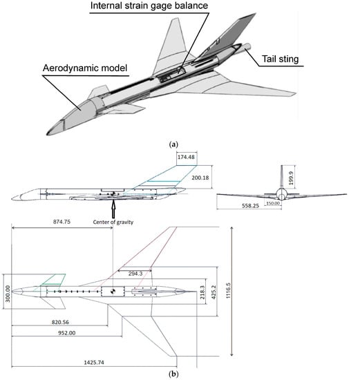
Figure 1.
TCR aircraft model (a) 3D view of the model mounted on the supporting device; (b) 3 views of the model: side (up-left), front (up-right) and top (bottom).
The wind tunnel experimental campaign was carried out in three stages. The tests were performed with the model installed on the tail sting, with the bank angle being equal to 90° (Figure 2). At the first stage, the static aerodynamic characteristics in a wide range of angles of attack were studied. The incidence angle was varied from −10° to 40° with the step of 2°. The static experiments were performed for various configurations of the model, namely, with and without canard. For the full configuration the canard deflection angle varied from −30° to +10° with a step of 5°. Rotation of the wind tunnel turn table provided variation of the angle of attack. In steady experiments for each angle of attack data sampling time was 2 s and the sampling rate was 100 Hz.
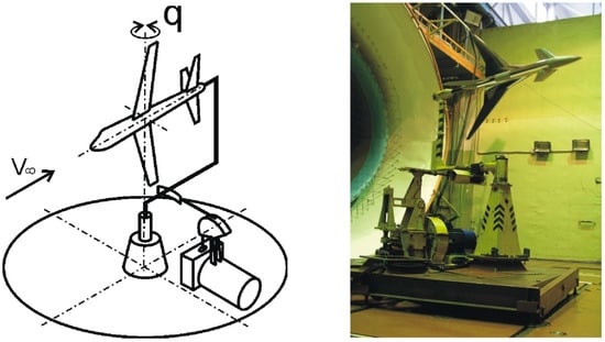
Figure 2.
Small-amplitude angular oscillations dynamic rig used in the TsAGI T-103 wind tunnel. The rig configuration is shown on the left, the TCR model inside the test section of the wind tunnel is shown on the right.
A five-component internal strain gauge balance was used for measurements of forces and moment acting on the aircraft model (a drag force was not measured). Reference point of the balance coincided with the model conventional center of gravity.
In the second stage, the stability derivatives were determined through the small-amplitude forced oscillations. During this experiment a harmonic motion in pitch with a fixed center of gravity is implemented:
The oscillation amplitude was , frequencies f were 0.5, 1.0, and 1.5 Hz (corresponding reduced frequencies were 0.012, 0.023, and 0.035) with the mean angles of attack varying from −10° to 40°. For small amplitude forced oscillation experiments the data were sampled 128 times per period of oscillation, each oscillation was repeated 8 times. No special adjustments of the sampling rates depending on the oscillation frequency were carried. These experiments were performed on the forced angular oscillations dynamic rig used in the TsAGI T-103 wind tunnel. The rig is shown in Figure 2. The rig kinematical scheme is shown on the left side, and the TCR model installed on the rig during the wind tunnel tests is shown on the right side. The mean angle of attack was specified with rotation of the wind tunnel turn table, and variation of the angle of attack was obtained via oscillation of the supporting sting.
In the third stage, nonlinear unsteady aerodynamic coefficients at high angles of attack were investigated through the large-amplitude forced oscillations in pitch. A view of the TCR model inside the wind tunnel during this stage is shown in Figure 3. These experiments were intended to obtain the additional experimental data for the more comprehensive models in the extended flight envelope.
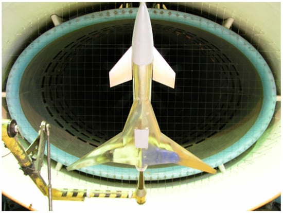
Figure 3.
TCR model at the large amplitude oscillation rig at wind tunnel test section.
The scheme of the rig is demonstrated in Figure 4. Kinematics is also given with the Equation (3). One can see from the figure that during these experiments the model bank angle was 0°. The mean angle of attack (3) was specified with an inclination of the sting support, and variation of the angle of attack was provided with oscillation of the sting with respect to its mean position. Oscillation amplitudes were 10° and 20°, frequencies were 0.5, 1, and 1.5 Hz (corresponding reduced frequencies k = 0.012, 0.023, and 0.035), and the mean angles of attack were 8° and 18°.
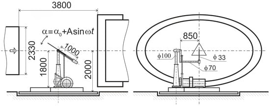
Figure 4.
Large-amplitude angular oscillations dynamic rig used in the TsAGI T-103 wind tunnel.
Data sampling rate was similar to the small-amplitude test rate, namely, 128 times per period, which is sufficient enough to capture abrupt variations of the measured aerodynamic characteristics during both types of the experiments. Each oscillation was repeated 16 times.
2.1. Static Aerodynamics Characteristics
The influence of the canard and canard deflection angle on the coefficients of normal force and pitching moment in steady conditions is shown in Figure 5. The analysis of the experiments shows that influence of the canard on the normal force coefficient CN is not so significant up to angle of attack α = 10°. At the angles of attack α > 10° the normal force is higher for the canard configurations. The detailed analysis in [23] reveals that, at small angles of attack, the wing in the presence of the canard has less slightly lift than a wing-only configurations; this is mainly due to canard downwash effects on the wing. However, the total lift remains the same because of the additional lift generated on the canard. At higher angles of attack, the wing behind the canard produces more lift than a wing-only geometry [23].
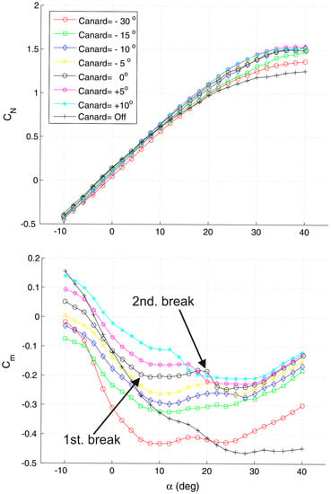
Figure 5.
Influence of the canard and canard deflection angle on the TCR aerodynamic characteristics.
The canard significantly contributes to the total pitching moment coefficient of the TCR model bringing a destabilizing effect. For the case of zero canard deflection, the pitching moment evolution with the angle of attack presents a negative slope (nose down when α increases) up to α = 6°, then a first break, after which the slope sign changes, due to the continuously increasing lift of the canard, upstream the reference point (nose up). Then a second break takes place, with a loss of efficiency at about α = 20°. The locations of these two breaks depend on the canard deflection angle.
Ghoreyshi et al. [23] reported some flow features of TCR at different angles of attack and at low subsonic speeds. Both the LEX, wing, and canard have rounded leading edges and are swept back at and more than 50°, that causes a complex vortex formation over these surfaces at moderate to high angles of attack. At about α = 12° a canard vortex and an inboard (LEX) and outboard wing vortex are present. The wing in the presence of the canard shows smaller inboard vortices than the canardless configuration; this is due to canard downwash effects that reduce the local angle of attack behind the canard span. On the other hand, the wing outboard vortex is slightly bigger in the presence of the canard. The canard vortex becomes larger with increasing angle of attack. At about α = 18° the wing vortices merge. At about α = 20°, the inboard and outboard vortices interact and merge. At α = 24° angle of attack, the canard vortex lifts up from the surface as well. At higher angles, the canard in the TCR aircraft has favorable effects on the wing aerodynamic performance.
2.2. Small-Amplitude Forced Oscillation Characteristics
The small amplitude oscillations are dedicated to determine the aerodynamic derivatives in Equation (1). The experimentally measured aerodynamic derivatives and are shown in Figure 6.
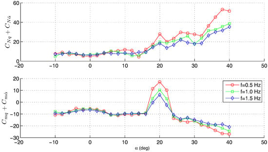
Figure 6.
Influence of the oscillation frequency on the unsteady derivatives and .
These dependencies were obtained at various frequencies of the aircraft model oscillations inside the wind tunnel. It is seen that the influence of the oscillation frequency on the aerodynamic derivatives is small, excluding the incidence region in the vicinity of α = 20°. In this region, a dependency of dynamic derivatives values versus the frequency of oscillations is observed. A comparison of the unsteady derivatives obtained for the canard and canardless configurations is given in Figure 7. The influence of the canard on the normal force derivative is significant for angles of attack larger than α = 32°; for pitch damping derivative it is also relatively small, except for the region of incidences near α = 20° (Figure 7), where a positive damping for the TCR model is observed.
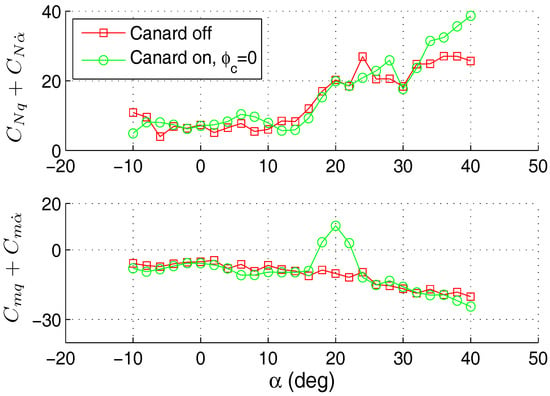
Figure 7.
Influence of canard on unsteady aerodynamic derivatives (k = 0.023).
The influence of the canard deflection angle was also investigated: the positive canard deflection moved the positive damping region to lower incidences, with the amplification of the phenomenon as compared to the case of (Figure 8). The negative canard deflection moved this region to higher angles of attack, with the positive damping being weakened. For the canard deflection angle , the positive damping moved to . For the normal force derivative, such a considerable effect is not observed.
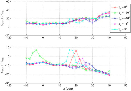
Figure 8.
Influence of canard deflection angle on pitch damping derivative (k = 0.023).
2.3. Large Amplitude Oscillations Characteristics
In order to investigate the vortex dynamics effect on unsteady aerodynamic characteristics at high angles of attack under high oscillation rates the large amplitude oscillations were carried out. As far as pitch oscillations were concerned, the canard-off TCR configuration revealed the classical linear dynamic effects without any strong nonlinearities. The addition of the canard leaded to severe unsteady effects, not only for angles of attack in the region of α = 20° but also for lower angles of attack (Figure 9).
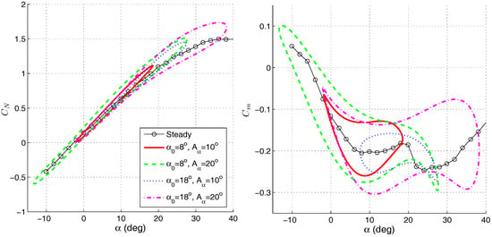
Figure 9.
Pitching moment and normal force coefficients evolutions for two sets of large amplitude pitch oscillations—TCR with canard, , k = 0.035.
3. Models of Unsteady Aerodynamic Characteristics
3.1. Aerodynamic Derivative Modeling
In order to quantify whether the linear model based on the look-up tables of aerodynamic derivatives is applicable the large amplitude oscillations results are simulated. Since the linear mathematical model in Form of Equation (1) is not valid for the large deviations from the trim incidence the mathematical model is written in the following form:
where , and are derived from the look-up tables of characteristics through the linear approximation. While modeling large-amplitude oscillations, the complexes and determined for the same oscillation frequency are used. The results of simulation large amplitude pitch oscillations are shown in Figure 10. One can see that the large amplitude oscillation results for the normal force coefficient can be described with a good precision using the look-up table approach. However, while the simulation of the pitching moment coefficient evolutions fits sufficiently well with the experimental data practically in the overall range of angle-of-attack range, there is a region of the incidences in the vicinity of α = 20°, for which this approach is failed to predict the experimental results. These modeling results are in good agreement with the small-amplitude test data given in Figure 6. Particularly, one can see that canard introduce the nonlinear behavior mostly for the pitching moment derivative , while it effect on the normal force derivative is not so vivid. The canard influence is observed in the vicinity of α = 20°, where the nonlinear dependency of the pitch moment derivatives on pitch rate is observed in the experiment (Figure 6), and the linear model failed to describe the experimental results.
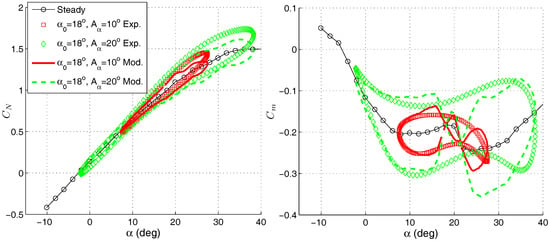
Figure 10.
Linear simulations based on the measured aerodynamic derivatives compared to large amplitude oscillation measurements.
Thus, nonlinear approaches should be applied in order to design comprehensive models of the pitch moment coefficient. Below, the NN approach will be used for modeling of unsteady aerodynamics under such conditions. In order to evaluate performance of the NN models they are compared with the state-space modeling approach [17].
3.2. State-Space Model
The state-space model of the pitch moment coefficient was developed through an analysis of the obtained experimental data. The pitch moment coefficient of the TCR model is considered as a sum of the pitching moment of the canardless configuration and the corresponding contribution from the canard as
The canard contribution under the static condition is divided into a term , which is linear in angle of attack, and a nonlinear term which is caused by the canard influence as follows:
This representation of the pitch moment coefficient is demonstrated in Figure 11. In the present study an unknown constant of the mathematical model and nonlinear function were determined using the static test results.
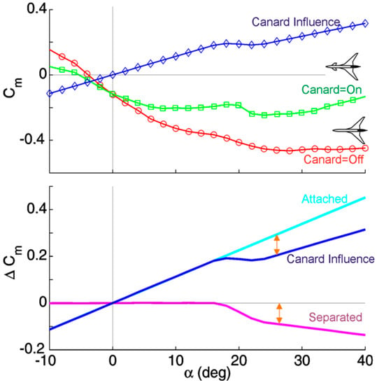
Figure 11.
The pitch moment coefficient representation.
In order to describe the internal dynamics due to the vortex structure development the following dynamic equation is applied:
where is the dynamic value of the canard influence due to development of vortex structure, and is its steady-state value.
This equation is a first-order filter with the time constant , which is in the left side of this equation. Additionally, incidence delay is introduced in the function argument in the right-hand side of the equation. For small values of time delays it follows from Equation (7) that , which enables the steady dependences to be satisfied identically.
The resulting pitch moment coefficient model is the following:
The equation combines the linear terms derived from the look-up tables for the canardless and canard TCR configurations (the first, the second and the third terms) and the nonlinear term responsible for the canard influence (the forth terms). Thus, the complete model for the pitch moment coefficient contains Equations (7) and (8) with unknown constants and . The constants , and the nonlinear function were determined by means of steady tests of the canardless and the canard configurations. The damping derivative is a function of the angle of attack and can be determined using the experimental results of the small-amplitude forced oscillations of the canardless TCR configuration.
For identification of the unknown parameters and the experimental results of small-amplitude pitch oscillations of the canard configuration of TCR model at various frequencies were used. The solution of Equation (7) for the small-amplitude harmonic oscillations in pitch can be linearized. After the substitution of the results into relationship (8) it leads to the following expressions for the aerodynamic derivatives:
It is seen that the aerodynamic derivatives depend on the oscillation frequency in the range of the angles of attack where the nonzero derivative exists. The dependencies of aerodynamic derivatives and versus oscillation frequency are determined by the characteristic times and . These values are supposed to be functions of the angle of attack and determined as the smooth cubic spline interpolations in the range of with the spline maximum in the center of the range (see Figure 9). It is considered that (α) = 0 beyond this range. The same assumption for leads to the degeneracy of differential Equation (4); therefore, = 2 is added to the spline function . This small addition does not influence significantly the filter characteristics in the left side of Equation (4), but enables the coefficient in front of derivative to be positive. For identification of these constants the following penalty function is introduced:
This function represents the sum of squared differences between the simulation results and the experimental results for the dynamic derivatives, determined in the entire investigated range of angles of attack αi for three values of the reduced oscillation frequency . For short, the designation is introduced in the expression. To determine the values of and the function should be minimized. It is seen in Figure 12 that this function has a flat minimum, which can be found using the conventional minimization techniques. The resulting functions () and () are shown in Figure 12.
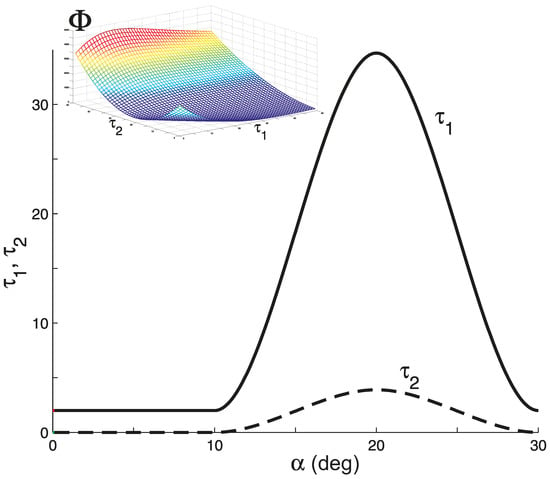
Figure 12.
The results of identification of and . Penalty function is shown in the upper left part of the figure.
The aerodynamic derivatives and versus angles of attack, simulated with the proposed mathematical model, are shown in Figure 13 with lines. The simulation results for various oscillation frequencies are demonstrated by lines of different types. The corresponding experimental results are shown with different markers. The developed state-space model describes adequately the results observed in the dynamic experiment in the entire ranges of the angles of attack and oscillation frequencies. It is important that the model describes the positive damping zone within the range of the angles of attack of α = 15–25° and the dependencies of the derivatives versus oscillation frequency, which are observed in the experiment.
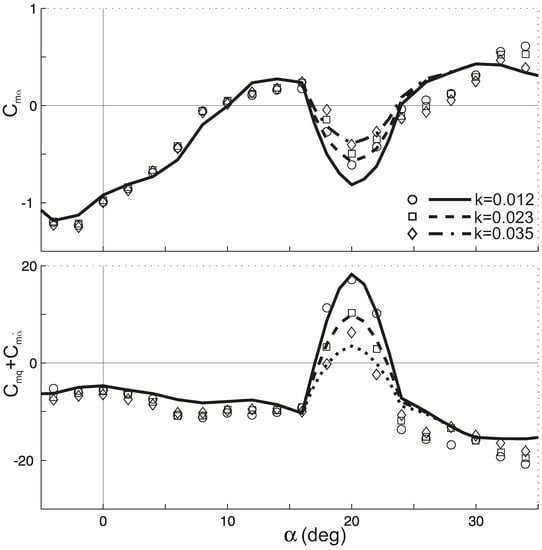
Figure 13.
Aerodynamic derivatives obtained for different oscillation frequencies: experiments (markers) and state-space model simulation (lines).
The state-space model (Equations (7) and (8)) developed only with the data from the forced small-amplitude oscillation tests was also applied to simulate the forced large-amplitude oscillations. The results obtained for three test cases are shown in Figure 14. The results of simulation (solid lines) and the unsteady experiment data (markers) for the dynamic values of are compared in the upper plots. The measured static values of are shown with dashed lines. The evaluations of dynamic components caused by the canard vortex flow formation (solid lines) are shown in the bottom plots. The static components of the vortex flow influence are shown with dashed lines in the same plots. The bottom graphs demonstrate the contribution of the differential equation with delay (Equation (7)) to the general mathematical model (Equation (8)).
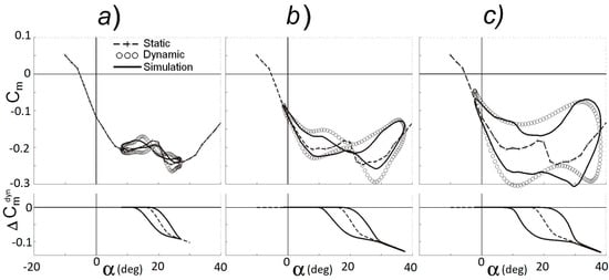
Figure 14.
Simulation results for the forced pitch oscillations with large amplitude: (a) (b) (c) .
The modeling results of the dynamic effects at the mean angle of attack of the pitch oscillations with large amplitude and small reduced frequency k = 0.012 are shown in Figure 14a. The positive damping in the sense of the linear mathematical model (1) is observed at angles of attack in the vicinity of . The additional kink in the dynamic loop demonstrates this fact. While the oscillation amplitude increasing, the positive damping practically vanishes in both the experiment and the simulation (see Figure 14b). Further oscillation frequency growth leads to a significant expansion of the hysteresis loop. This effect in the experimental and simulation results is shown in Figure 14c.
The NN techniques described and applied below are compared with the state-space approach.
4. Neural Network Modeling
FFNN and RNN are considered in the paper. The NN model of unsteady pitch moment coefficient of TCR using RNN was developed in this paper and compared with the model obtained using FFNN [19].
4.1. NN Architectures
The FFNN, which scheme is given in Figure 15a, can be considered as a directed graph with neurons placed in it nodes. The neurons of the first layer do not implement nonlinear mapping but distribute input signals between neurons of the first hidden layer. Neuron of the hidden layer is an elementary calculating unit. A set of signals from the input layer are fed into the neuron of the hidden layer. Coefficients correspond to the signal transmit connections and are the weight factor while summing the input signals. Neuron bias is added to the weighted sum of the input signals, and the resulting sum is mapped through nonlinear activation function . Mapped signal goes forward to the next-layer neurons, which implement the same operations and transmit the signal further. The signal from the last layer is output from the NN.
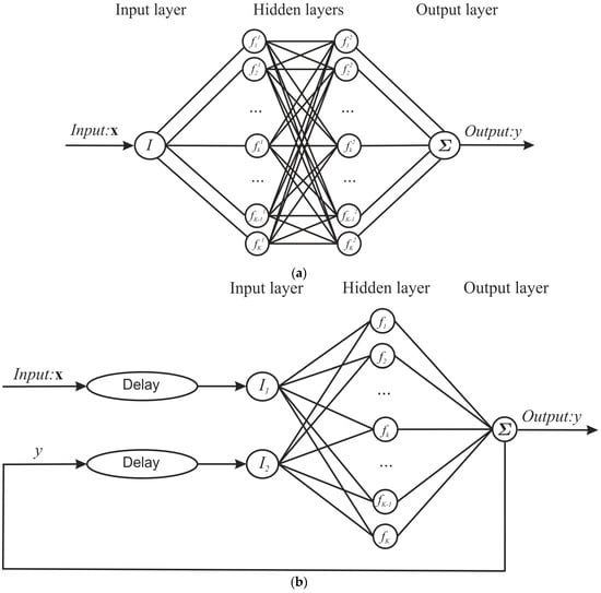
Figure 15.
NN architectures: (a) FFNN architecture; (b) NARX architecture.
RNN can be represented as FFNN with feedback connections. NARX (Nonlinear AutoRegressive model with eXogenous variables) architecture [32], which is given in Figure 15b, is used in the present study. For modeling variable y at time t, the state vector and a series of its former values are fed into the NN. The values of the modeling variable calculated by the NN earlier are also added to input signal. The resulting NN model can be presented in the following form:
where M is the function of NN mapping.
4.2. Regularization Techniques during NN Training
The problem considered in the present study is to develop a NN model using a restricted set of experimental data and to apply the model for flight dynamics applications, implying arbitrarily aircraft maneuvers; thus, generalization ability of the model is crucial. Regularization is one of the popular techniques preventing overfitting of a regression model and improving its generalization ability [33]. A short introduction to regularization techniques is given below.
Connection weights and biases are adjusted during NN training when the examples of training set are presented through minimization of the difference between NN operation results yi and target value ai for each example () from the training set
One of the important problems of NN training is called overfitting. The error in the training set is driven to a very small value, but when new data are presented to the network the error is large. The network has memorized the training examples, but it has not learned to generalize to new situations. A part of the whole initial data can be used for model testing. The test set error should be made as small as possible and must not be significantly higher than the training set error. When this condition is valid, the NN is considered to have good generalization performance.
Regularization is one of the techniques for improving generalization. According to this technique, a term penalizing the NN for weight increase is added in the objective function besides the error measure (12). The sum of squares of the weights can be used for this purpose:
where K is a number of neural network weights; the objective function takes the form
where and are objective function parameters. To develop the mathematical model with high generalization ability, Bayes’ rule was proposed to define the objective function parameters [34]. Algorithm of Gauss–Newton approximation to Bayesian regularization (GNBR) for training NN was further implemented in [33].
GNBR algorithm is the effective tool to improve NN generalization, but it supposes the model error to be the same on different subsets of initial data. The unsteady aerodynamic models for flight dynamics problems are developed using different dynamic experiments, in the various ranges of kinematic parameters, and with different accuracies. To obtain more precise models the data could be considered as heteroscedastic. The GNBR algorithm was modified for the case of heteroscedastic data and Bayesian Regularization to NN training on Heteroscedastic Data (BRHD) was proposed [35]. Below the proposed algorithm is briefly discussed.
4.3. Bayesian Regularization to NN Training on Heteroscedastic Data (BRHD)
Let us suppose that experimental data to be approximated are obtained in n types of different experiments , where is the vector of values of the controlled phenomenon parameter, obtained in i-th type of experiment, is the vector of values of the observed variable obtained in i-th type of experiment, is the dataset obtained at the same type of experiment.
The problem is to identify the NN function y that describes the obtained experimental data :
The errors in each experiment , are supposed to be independent and normal with zero statistical expectation but with different standard deviations . Using Bayes’ rule, the following objective function can be obtained:
where is the vector of weights, is the vector of errors, is the error of approximation of j-th data pair, R is the matrix N × N; the objective function parameters are placed on the main diagonal of matrix R, the other elements of this matrix are equal to zero:
Note that the objective function in form (16), which is used instead of (14), contains the weighted sum of errors on each subset , with weights , corresponding to each subset. Following Bayes’ rule, the expressions for the objective function parameter (16) is obtained [35]:
where K is the total number of parameters in the network, is the Hessian matrix of the objective function, and Sp is the matrix trace.
The following expressions can be obtained for :
where is the number of patterns of the i-th training subset.
Within this approach, the parameters of the objective function corresponding to the data subset are adjusted subject to their approximation errors.
The algorithm for implementation of the described training technique was developed [35]. To obtain values of the objective function parameters it is required to calculate Hessian matrix in the minimum point of objective function F. The Gauss–Newton method is applied to approximate Hessian matrix with modified Levenberg–Marquardt optimization algorithm used to locate the minimum point:
Let us consider the Levenberg–Marquardt algorithm in more detail. When the scalar μ is zero, this is just Newton’s method, using the approximate Hessian matrix. When μ is large, this becomes gradient descent with a small step size. Newton’s method is faster and more accurate near an error minimum, so the aim is to shift toward Newton’s method as quickly as possible. Thus, μ is decreased after each successful step (reduction in performance function) and is increased only when a tentative step would increase the performance function. In this way, the performance function is always reduced at each iteration of the algorithm [36].
The modification proposed in the present paper improves the Levenberg–Marquardt algorithm convergence in the case of heteroscedastic data in the vicinity of the minimum point.
4.4. Modeling
The RNN model of unsteady pitch moment coefficient, which has a NARX configuration, is compared with the FFNN model presented in [26]. The RNN has one hidden layer. RNN containing from five to 20 neurons in the hidden layer were tested and 12 neurons were selected because this number provides better generalization. Hidden layer neurons have a sigmoid activation function:
Experimental data, which are used to train the NN, consisted of the oscillation cases corresponding to different amplitudes and frequencies of oscillation. Evolutions of the pitch moment coefficient and kinematic parameters during each oscillating case are discretized in time into 128 steps both for small- and large-amplitude tests. Small-amplitude oscillation cases total 78; large-amplitude oscillation cases total 12. The training patterns are composed of the target data, which are the records of pitch moment coefficient at steps i, i − 1, together with the input vector. In the present study the input vector included the angle of attack and pitch rate at the i-th step, and the motion parameters , at previous steps i − 1, i − 2. Usage of angle of attack and pitch rate as the main input parameters is motivated by the statement of the problem. Namely, the developed NN model should be used for flight dynamics problems, and, hence, we should use only parameters available during a real flight. Influence of the Mach and Reynolds numbers are not considered in the present experimental study and, hence, are not included in the NN model as the input parameters.
To compare only the NN configurations, the regularization technique (GNBR) is selected to be the same as for FFNN in [26].
To train the RNN, a special configuration can be used. Because the true output is available during the training of the network, it is possible to create a feed-forward architecture, in which the true output is used instead of feeding back the estimated output. This has two advantages. The first is that the input to the feed-forward network is more accurate. The second is that the resulting network has a purely feed-forward architecture, and static back propagation can be used for training [32]. The stopping criterion for training was exceeding a threshold value (1020) by the Levenberg–Marquardt algorithm parameter µ, which corresponded to reaching a minimum of the objective function (16).
Thirty-six out of 78 small amplitude test cases and eight out of 12 large amplitude test cases were randomly selected for training; the rest of the data were used for testing.
At the modeling stage, predicting the pitch moment coefficient RNN uses results computed at the previous time step , along with the current and two previous steps of input signal. Hereby, the model is a nonlinear regression on seven parameters. As is shown in [26], a six-dimensional state vector is enough to specify the harmonic oscillation process.
In the first step, we simulated the aerodynamic derivatives of pitch moment coefficient (1). They were obtained with RNN as follows. First, the forced small-amplitude oscillations of the aircraft model were simulated. Then, the coefficients of the model (1) were identified from the simulated data using the linear regression method. RNN simulation of the pitch moment derivatives, compared with the small-amplitude experiment, is given in Figure 16. It can be seen from the figure that the RNN model captures the dependency of the derivatives on oscillation frequency, which is observed in the angle-of-attack range and corresponds to the development of the vortical flow above the wing surface. Here the results from both the training and testing subsets are demonstrated together in order to illustrate that the developed model describes all available small-amplitude test results and can be used for prediction of the unsteady aerodynamics phenomena in the overall studied angle-of-attack range. Nevertheless, a detailed study of the model performance on both training and test subsets is given in Section 4.
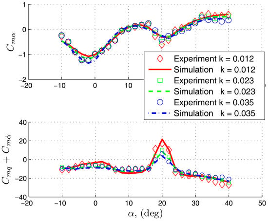
Figure 16.
Unsteady aerodynamic derivatives of the pitch moment coefficient, simulated with RNN (lines) and obtained in the experiment (markers).
Hysteresises of the pitch moment coefficient obtained by the RNN simulation of the forced large-amplitude oscillations are given in Figure 17. The experimental results are also plotted in the same figure. These cases are from the testing subset. One can see that there is a good correlation between the experiment and the simulation, and a good generalization is exhibited by RNN.
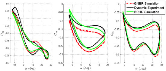
Figure 17.
Forced large-amplitude oscillation results for the pitch moment coefficient.
It can be concluded from Figure 16 and Figure 17 that RNN describes the nonlinear behavior of the pitch moment coefficient in the extended range of the angles of attack, which are observed in the experiments.
FFNN, developed in [26], had two hidden layers, with 12 neurons in the first layer and seven in the second. The neuron activation function of the both layers was also chosen sigmoid function. Patterns for the training of the FFNN were composed of the records of pitch moment coefficient , together with the state input determined for the oscillation case. Each oscillating case was discretized in time into 128 steps (similar to the experiment data) and readings from a strain-gauge balance were used for each step. Two thirds of the experimental data were used to train the neural network, and one third of the experimental data were used to test the generalization ability. To simulate the pitch moment coefficient at the time t of an experiment case the whole input vector at this time step should be fed in the NN.
Backpropagation was used to train the NN. Levenberg–Marcquardt algorithm, combined with Bayesian regularization (GNBR), was utilized to minimize the error [26]. The following section gives a comparison of the performance of the discussed NN models.
5. Comparison of the Models
First, let us compare the NN models. The performances of the NN models were tested quantitatively by calculating the errors obtained for the models of pitch moment coefficient and the complex of aerodynamic derivatives separately for the train and test subsets. The error measure is the mean square error divided by the entire range of the measured value :
The results are given in Table 1.

Table 1.
Errors of unsteady aerodynamics models.
Considering the table, one can conclude that the FFNN error for the small amplitude test is approximately the same as for the training and testing subsets. The error for the large amplitude test is very high, approximately four times higher for the training subset and seven times higher for the test subset as compared with the small-amplitude results. Thus, the FFNN provides worse performance for the large amplitude subset. The reason is that the small-amplitude training examples are dominant in the overall training set, namely, 36 out of 44 cases. The FFNN trained better to model the small-amplitude behavior shows poor performance for the large-amplitude subset. This is not satisfactory from the point of view of flight dynamics because a model should guarantee an equal level of model precision in the overall simulation domain.
On the contrary, errors of the RNN determined for small- and large-amplitude subsets are not as high as the FFNN large-amplitude errors and are very close to each other, especially for the testing subsets. This indicates that the RNN is trained to model both small- and large-amplitude results almost equivalently and the shortcomings of the FFNN have been overcome.
Another important remark should be given while comparing the FFNN and RNN architectures. In addition to the aforementioned advantage of RNN, there is another one. It is possible to simulate any consequence of time-dependent states using the RNN thanks to the feedback connection. On the contrary, while using FFNN one should input all parameters of the oscillation cycle, including amplitude and frequency of oscillation, which is not suitable for flight dynamics applications. This comparison reveals that the recurrent configuration is a favorable technique for the simulations of time-dependent unsteady aerodynamic characteristics in flight dynamics problems.
Unsteady aerodynamic characteristics obtained in different types of the experiments are obtained with different errors. Performances of the mathematical models are improved using the BRHD technique that considers the model developed using the experiment data from different types of experiments as heteroskedastic [27].
While comparing the regularization techniques, the recurrent architecture was used because in the previous section this NN configuration was shown to be better for the problem of modeling of aerodynamics in flight dynamics than the feed-forward architecture. The NN was trained using both the GNBR and the BRHD algorithms on the same data. For the BRHD, 8 neurons in the hidden layer were selected, i.e., it is less than for GNBR (12 neurons). The model performances were compared in several ways. First, the testing was done graphically by coplotting values measured in the experiment and predicted by the models. The results of large-amplitude modeling are shown in Figure 17, where it can be concluded that the NN model, trained with the BRHD algorithm, has better coincidence with the experiments.
More thorough analysis of the obtained results was implemented to determine whether the BRHD algorithm helped to improve accuracy of models derived from the different-type experiment data. For this purpose, the NN models of TCR pitch moment coefficient, obtained using the BRHD and GNBR training algorithms were compared. A quantitative comparison of the training techniques was done in the same way as for the configuration comparison through the error calculation (22). The results are also given in Table 1. The comparison reveals the accuracy improvement of the model developed with BRHD. The errors for decreased by 23% and 31% for the train and test subsets, respectively. The errors for decreased by 25% and 49% for the train and test subsets, respectively.
In addition, the scatterograms plotted for the test subsets of and are shown in Figure 18a,b. The BRHD technique yields less scattering.
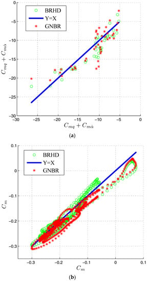
Figure 18.
Scattering diagrams: test subsets: (a) Small amplitude subtest; (b) large amplitude subtest.
The analysis presented above shows that the regularization technique (BRHD) improves the model accuracy if two or more subsets obtained in different experiments are used to train the NN.
The error of the state-space model, which is calculated according to Equation (22) in order to evaluate the performance of the NN modeling approach, is given in Table 1. The RNN trained with the conventional GNBR algorithm shows better accuracy as compared to the state-space model for small amplitudes, and for the large-amplitude tests the performance of the RNN (GNBR) is better in the training test and worse in the testing subset. The RNN (BRHD) has better precision for both small- and large-amplitude oscillation data.
6. Conclusions
An experimental investigation of the aerodynamic characteristics of the prospective civil transport aircraft TCR has been carried out in the TsAGI T-103 wind tunnel. The aircraft was a configuration with a high-sweep wing with LEX and the high-sweep canard surface. A three-stage experimental campaign was undertaken. In the first stage, the steady aerodynamic characteristics were under consideration. The influence of the reduced oscillation frequency and the angle of attack on unsteady aerodynamic derivatives was studied in the second stage. In the third stage, forced large-amplitude oscillation tests were carried out for the detailed investigation of the unsteady aerodynamics at high-angle-of-attack departures. The analysis of the experiments revealed that canard had a great impact on the overall aircraft performance. Static experimental results showed that the influence of the canard on the normal force coefficient CN was not so significant up to the angle of attack α = 10°. At angles of attack α > 10° the normal force was higher for the canard configurations. Such behavior at high angles of attack was due to the fact that the wing behind the canard produced more lift than a wing-only geometry because of the canard–wing vortex interaction.
The canard also significantly contributed to the total pitching moment coefficient of the TCR model, making it less stable. In addition, canard-wing vortex interaction phenomena caused the positive damping peak in the stability derivative obtained in a small-amplitude forced oscillation experiment, which was not observed for the wing-only configuration. Changing the canard deflection angle , one could change the position and amplification of the positive damping peak.
Concerning large-amplitude forced oscillations, the wing-only configuration revealed the classical linear dynamic effects without strong nonlinearities. The addition of the canard led to severe unsteadiness in the form of hysteresises. The delay of complex vortical flow development caused the dependence of the aerodynamic derivatives on the oscillation frequency and the complicated hysteresis loops of the total pitch moment coefficient, observed in the large-amplitude oscillation.
While modeling large-amplitude oscillation results using the look-up tables approach, the large amplitude oscillation results for the normal force coefficient were described with good precision. However, for the pitch moment coefficient the technique failed and several more sophisticated mathematical models obtained via different popular approaches, namely, neural network and the phenomenological state-space modeling technique, were developed.
We compared several approaches for reduced-order modeling that are capable of capturing the observed nonlinear phenomena. In particular, NN of the feed-forward and recurrent architectures were compared with each other and with the state-space model. RNN trained with the BRHD algorithm showed better results in terms of prediction ability. Comparison of the NN models revealed that the recurrent architectures were favorable for modeling of unsteady aerodynamic characteristics in flight dynamics problems. The advantage of the RNN was the feedback connection, which provided prehistory of motion and brought the information required for modeling dynamic processes. In addition, RNN demonstrated better generalization ability, which was an important advantage because the ROM of aerodynamics were designed with a restricted set of kinematic parameters, which could be obtained in the wind tunnel or CFD tests. However, solving of flight dynamic problems, including ground-based simulator studies, supposes simulation of arbitrary aircraft maneuvers.
Acknowledgments
This work has been carried out with funding from the Russian Ministry of Education and Science into the subject “Applying artificial neural networks to promote flight safety,” project 14.624.21.0046.
Author Contributions
Dmitry Ignatyev and Alexander Khrabrov conducted the experiments; Dmitry Ignatyev developed NN models; Alexander Khrabrov developed state-space model, Dmitry Ignatyev and Alexander Khrabrov analyzed the data, Dmitry Ignatyev wrote the paper.
Conflicts of Interest
The authors declare no conflict of interest.
Nomenclature
| amplitude of oscillation | |
| yi | neural network operation results |
| ai | target value |
| wing span | |
| neuron bias | |
| pitch moment coefficient | |
| mean aerodynamic chord | |
| sum of squared neural network errors | |
| sum of squared neural network weights | |
| neural network error | |
| error measure | |
| objective function | |
| neuron activation function | |
| H | Hessian matrix |
| J | Jacoby matrix |
| k | reduced oscillation frequency |
| function of neural network operations | |
| input signals fed into neuron | |
| t | time |
| airspeed | |
| weights of the neural network connections | |
| angle of attack | |
| mean angle of attack at the oscillations | |
| , | objective function parameters |
| canard deflection angle | |
| τ1, τ2 | characteristic times |
| signal mapped by the neuron | |
| Subscripts | |
| dyn | dynamic |
| sep | separated |
| sim | simulation |
| st | static |
| test | testing |
| T | transpose |
| Aerodynamic derivatives | |
| , where i = N, m. | |
References
- European Aviation Safety Agency. Annual Safety Review 2011. Available online: https://www.easa.europa.eu/communications/docs/annual-safety-review/2011/EASA-Annual-Safety-Review-2011.pdf (accessed on 2 April 2014).
- Ignatyev, D.I.; Sidoryuk, M.E.; Kolinko, K.A.; Khrabrov, A.N. Dynamic Rig for Validation of Control Algorithms at High Angles of Attack. J. Aircr. 2017, 54, 1760–1771. [Google Scholar] [CrossRef]
- Abramov, N.B.; Goman, M.G.; Khrabrov, A.N.; Kolesnikov, E.N.; Fucke, L.; Soemarwoto, B.; Smaili, H. Pushing ahead—SUPRA airplane model for upset recovery. In Proceedings of the AIAA Modelling and Simulation Technologies Conference (AIAA 2012-4631), Minneapolis, MN, USA, 13–16 August 2012; American Institute of Aeronautics and Astronautics: Reston, VA, USA, 2012. [Google Scholar] [CrossRef]
- Foster, J.V.; Cunningham, K.; Fremaux, C.M.; Shah, G.H.; Stewart, E.C.; Rivers, R.A.; Wilborn, J.E.; Gato, W. Dynamics modelling and simulation of large transport airplanes in upset conditions. In Proceedings of the AIAA Atmospheric Flight Mechanics Conference and Exhibit (AIAA-2005-5933), San Francisco, CA, USA, 15–18 August 2005; American Institute of Aeronautics and Astronautics: Reston, VA, USA, 2005. [Google Scholar] [CrossRef]
- Da Ronch, A.; Vallespin, D.; Ghoreyshi, M.; Badcock, K.J. Evaluation of dynamic derivatives using computational fluid dynamics. AIAA J. 2012, 50, 470–484. [Google Scholar] [CrossRef]
- Harrison, S.; Darragh, R.; Hamlington, P.; Ghoreyshi, M.; Lofthouse, A. Canard-wing interference effects on the flight characteristics of a transonic passenger aircraft. In Proceedings of the 34th AIAA Applied Aerodynamics Conference, AIAA AVIATION Forum (Paper 2016-4179), Washington, DC, USA, 13–17 June 2016; American Institute of Aeronautics and Astronautics: Reston, VA, USA, 2016. [Google Scholar] [CrossRef]
- Sereez, M.; Abramov, N.; Goman, M. Computational Ground Effect Aerodynamics and Airplane Stability Analysis during Take-Off and Landing. In Proceedings of the 7th European Conference for Aeronautics and Aerospace Sciences (EUCASS), Milan, Italy, 3–6 July 2017. [Google Scholar] [CrossRef]
- Schütte, A.; Einarsson, G.; Raichle, A.; Schoning, B.; Mönnich, W.; Forkert, T. Numerical simulation of maneuvering aircraft by aerodynamic, flight mechanics and structural mechanics coupling. J. Aircr. 2009, 46, 53–64. [Google Scholar] [CrossRef]
- Ghoreyshi, M.; Cummings, R.; Da Ronch, A.; Badcock, K. Transonic aerodynamic load modelling of X-31 aircraft pitching motions. AIAA J. 2013, 51, 2447–2464. [Google Scholar] [CrossRef]
- Ghoreyshi, M.; Jirásek, A.; Cummings, R. Computational approximation of nonlinear unsteady aerodynamics using an aerodynamic model hierarchy. Aerosp. Sci. Technol. 2013, 28, 133–144. [Google Scholar] [CrossRef]
- Zaichik, L.; Yashin, Y.; Desyatnik, P.; Smaili, H. Some aspects of upset recovering simulation on hexapod simulators. In Proceedings of the AIAA Modelling and Simulation Technologies Conference, Guidance, Navigation, and Control and Co-Located Conferences (AIAA Paper 2012-4949), Minneapolis, MN, USA, 13–16 August 2012; American Institute of Aeronautics and Astronautics: Reston, VA, USA, 2012. [Google Scholar] [CrossRef]
- Bushgens, G.S. (Ed.) Aerodynamics, Stability and Controllability of Supersonic Aircraft; Nauka, Fizmatlit: Moscow, Russia, 1998; 816p. (In Russian) [Google Scholar]
- Etkin, B. Dynamics of Atmospheric Flight; Wiley: New York, NY, USA, 1972; pp. 101–114, 129–154, 219–256, 280–295. [Google Scholar]
- Tobak, M.; Schiff, L.B. On the Formulation of the Aerodynamic Characteristics in Aircraft Dynamic; NASA TR R-456; National Aeronautic and Space Administration: Washington, DC, USA, 1976.
- Klein, V.; Noderer, K.D. Modelling of Aircraft Unsteady Aerodynamic Characteristics. Part 1—Postulated Models; NASA Technical Memorandum 109120; Langley Research Center: Hampton, VA, USA, 1994.
- Huang, X.Z.; Lou, H.Y.; Hanf, E.S. Airload Prediction for Delta Wings at High Incidence; ICAS Paper. In Proceedings of the 22nd Congress of the Aeronautical Sciences, Harrogate, UK, 27 August–1 September 2000; pp. 221.1–221.10. [Google Scholar]
- Goman, M.G.; Khrabrov, A.N. Space representation of aerodynamic characteristics of an aircraft at high angles attack. J. Aircr. 1994, 31, 1109–1115. [Google Scholar] [CrossRef]
- Jumper, E.J.; Schreck, S.J.; Dimmick, R.L. Lift-curve characteristics for an airfoil pitching at constant rate. J. Aircr. 1987, 24, 680–687. [Google Scholar] [CrossRef]
- Ioselevich, A.S.; Stolyarov, G.I.; Tabachnikov, V.G.; Zhuk, A.N. Experimental Investigation of Delta Wing A = 1.5 Damping in Roll and Pitch at High Angles of Attack. Proc. TsAGI 1985, 2290, 52–70. [Google Scholar]
- Abramov, N.; Goman, M.; Greenwell, D.; Khrabrov, A. Two-step linear regression method for identification of high incidence unsteady aerodynamic model. In Proceedings of the AIAA Atmospheric Flight Mechanics Conference (Paper 2001-4080), Montreal, QC, Canada, 6–9 August 2001. [Google Scholar] [CrossRef]
- Vinogradov, Y.A.; Zhuk, A.N.; Kolinko, K.A.; Khrabrov, A.N. Mathematical simulation of dynamic effects of unsteady aerodynamics due to canard flow separation delay. TsAGI Sci. J. 2011, 42, 655–668. [Google Scholar] [CrossRef]
- Luchtenburg, D.M.; Rowley, C.W.; Lohry, M.W.; Martinelli, L.; Stengel, R.F. Unsteady high-angle-of-attack aerodynamic models of a generic jet transport. AIAA J. Aircr. 2015, 52, 890–895. [Google Scholar] [CrossRef]
- Faller, W.E.; Schreck, S.J.; Helin, H.E. Real-time model of three dimensional dynamic reattachment using neural networks. J. Aircr. 1995, 32, 1177–1182. [Google Scholar] [CrossRef]
- Faller, W.E.; Schreck, S.J. Unsteady fluid mechanics applications of neural networks. J. Aircr. 1997, 34, 48–55. [Google Scholar] [CrossRef]
- Reisenthel, P.H. Development of nonlinear indicial model using response functions generated by a neural network. In Proceedings of the 35th Aerospace Sciences Meeting and Exhibit (AIAA 97-0337), Reno, NV, USA, 6–9 January 1997. [Google Scholar] [CrossRef][Green Version]
- Ignatyev, D.I.; Khrabrov, A.N. Application of neural networks in the simulation of dynamic effects of canard aircraft aerodynamics. TsAGI Sci. J. 2011, 42, 817–828. [Google Scholar] [CrossRef]
- Ignatyev, D.I.; Khrabrov, A.N. Neural network modelling of unsteady aerodynamic characteristics at high angles of attack. Aerosp. Sci. Technol. 2015, 41, 106–115. [Google Scholar] [CrossRef]
- Glaz, B.; Liu, L.; Friedmann, P. Reduced-order nonlinear unsteady aerodynamic modelling using a surrogate-based recurrence framework. AIAA J. 2010, 48, 2418–2429. [Google Scholar] [CrossRef]
- Kolmogorov, A.T. On the Representation of Continuous Functions of Many Variables by Superposition of Continuous Functions of One Variable and Addition; American Mathematical Society Translations: Providence, RI, USA, 1963; Volume 28, pp. 55–59. [Google Scholar]
- Mialon, В.; Khrabrov, A.; Da Ronch, A.; Cavagna, L.; Zhang, M.; Ricci, S. Benchmarking the prediction of dynamic derivatives: Wind tunnel tests, validation, acceleration methods. In Proceedings of the AIAA Atmospheric Flight Mechanic Conference (AIAA Paper 2010-8244), Toronto, ON, Canada, 2–5 August 2010. [Google Scholar] [CrossRef][Green Version]
- Ghoreyshi, M.; Korkis-Kanaan, R.; Jirásek, A.; Cummings, R.; Lofthouse, A. Simulation validation of static and forced motion flow physics of a canard configured TransCruiser. Aerospace Sci. Technol. 2016, 48, 158–177. [Google Scholar] [CrossRef]
- Hagan, M.T.; Demuth, H.B.; Beale, M.H. Neural Network Design; PWS Publishing: Boston, MA, USA, 1996. [Google Scholar]
- Foresee, F.D.; Hagan, M.T. Gauss-Newton approximation to Bayesian regularization. In Proceedings of the International Joint Conference on Neural Networks, Houston, TX, USA, 12 June 1997; pp. 1930–1935. [Google Scholar] [CrossRef]
- MacKay, D.J.C. Bayesian Interpolation. Neural Comput. 1992, 4, 415–447. [Google Scholar] [CrossRef]
- Ignatyev, D.I.; Khrabrov, A.N. Neural network modelling of longitudinal aerodynamic characteristics of aircraft. Informatsionnye Tekhnologii 2014, 3, 61–69. [Google Scholar]
- Hagan, M.T.; Menhaj, M. Training feed-forward networks with the Marquardt algorithm. IEEE Trans. Neural Netw. 1994, 5, 989–993. [Google Scholar] [CrossRef] [PubMed]
© 2018 by the authors. Licensee MDPI, Basel, Switzerland. This article is an open access article distributed under the terms and conditions of the Creative Commons Attribution (CC BY) license (http://creativecommons.org/licenses/by/4.0/).