Abstract
Aircraft spin, a nonlinear phenomenon dominated by unsteady aerodynamics, is difficult to predict. This article proposes a novel approach using Hankel Dynamic Mode Decomposition with Control (HDMDc) to identify an aircraft plant model for spin motion directly from measurement data. A key challenge in real-world data-driven modeling is addressing noise in both input and output measurements, often termed errors in variables (EIV). The standard HDMDc does not account for the distinct noise characteristics of different sensors. To overcome this, modifications are proposed to the standard HDMDc algorithm using EIV approaches: total least squares and bias-eliminating least squares. The proposed algorithms are validated first with a simple nonlinear dynamical system exhibiting limit cycle oscillation. Further, the methodology is applied to the simulated steady spin of the T-2 aircraft and the oscillatory spin motion of the F-18 aircraft. It is demonstrated that models identified using HDMDc with the EIV approach predicted spin trajectories with high goodness-of-fit values, even for unseen control inputs and initial conditions that differed from the training data. Specifically, the predicted trajectories had a FIT% close to 90% in most cases, with the worst-case FIT% being 38%. In contrast, the standard HDMDc algorithm’s predicted trajectory was not even visually close to the actual system trajectory, highlighting the significant improvement of the modified approach.
1. Introduction
Modeling of aircraft spin motion is difficult. The aerodynamic forces and moments experienced by the aircraft during the spin are nonlinear, coupled, and history dependent with respect to the aircraft states. This is because during spin, the airplane wings are stalled, leading to flow separation and unsteady aerodynamics. This nonlinearity occurs in addition to the kinematic nonlinearity in the equations of motion, such as inertial coupling [1].
The traditional method of modeling aircraft spin motion involves carrying out a series of wind tunnel experiments using scaled aircraft models to arrive at a model of aerodynamic forces and moments [2]. Forced oscillation tests are performed to estimate the aerodynamic damping derivatives. Further, the aircraft model is continuously rotated about the velocity vector in the wind tunnel through special mechanisms to arrive at rotary derivatives. These aerodynamic data are combined with static wind tunnel test data to arrive at an integrated model of aerodynamic forces and moments. The arrived aerodynamic model, combined with the aircraft equations of motion, can be used to estimate the aircraft spin modes.
The above methodology suffers from various disadvantages. First, a number of well-planned wind tunnel tests need to be carried out, which takes a considerable amount of time and effort. Further, the fidelity of the model, and therefore its capability to predict airplane trajectory during spin, is low. This is because the model assumes a superposition of the forces and moments. The aerodynamic derivatives are separately estimated for various airplane motions like pitch, roll, and yaw. However, during a spin, these motions are coupled, and the governing equations are nonlinear. That renders the methods based on superposition ineffective.
There is some literature that uses data collected in flight to arrive at an aircraft spin model. Gresham et al. [3] use the traditional equation error method to arrive at a nonlinear, coupled, quasi-steady aerodynamic model for spin using flight data. An RC-controlled E-flite Carbon-Z Cessna 150 (CZ150) model is used to collect in-flight data. The aircraft is made to enter a spin, and during the spin motion, multisine control surface excitations are given. The recorded flight data are used to arrive at rotary, damping, and control derivatives for modeling aerodynamic forces and moments. The equation error method provides a way to estimate the parameters of an assumed airplane model. Therefore, the model obtained is only as good as the model assumed. Given the complexity of spin dynamics and aerodynamics, it is difficult to come up with a good spin model to be used with the equation error method. Compared to the traditional force and moment spin model, the authors in [3] consider some additional stability and control derivatives. These terms are included based on the multivariate orthogonal function (MOF) modeling approach [4]. The MOF modeling approach was used to identify the dominant terms, whose inclusion in the model reduces the mean square fit error of the collected data. However, a drawback of this method is the need for an appropriate selection of basis functions, which can be challenging without sufficient prior knowledge of complex spin dynamics.
A difficulty associated with the modeling techniques employing the equation error method is the following. The equation error method requires the derivative of some of the measured quantities for state estimation. Using numerical differentiation of noisy measurements to obtain those leads to inaccurate models. Furthermore, in real flight data, the noise levels vary across different output measurements. In such a case, the equation error method, which employs least square estimation, may not yield consistent estimates of the coefficients/derivatives.
Mokhtari and Sabzehparvar [5] explore the use of ensemble empirical mode decomposition (EEMD) for modeling aerodynamic forces and moments. The authors use an extended multi-point modeling technique where forces and moments on each lifting surface are modeled. Flight data of V-tailed single-engine light aircraft are used. The recorded output data are decomposed into intrinsic mode functions (IMFs) using EEMD. These IMFs are then used as inputs for identifying the coefficients of the extended multi-point aerodynamic model. The disadvantage of this aerodynamic modeling approach is the large number of parameters and the requirement for aircraft geometry definition.
As an alternative to the above-mentioned estimation techniques, the estimation of the aircraft plant model for spin using Hankel dynamic mode decomposition with control (HDMDc) is explored in this article. The plant model arrived at using the HDMDc-based estimation is applicable only around a spin equilibrium point. Nonetheless, this model does not require the estimation of derivatives of measured noisy outputs as in the equation error method.
Dynamic Mode Decomposition with Control (DMDc) is a system identification method that uses measurement data to obtain an approximate linear time-invariant plant model with control in the output space [6,7]. DMDc has been used in various fields such as robotics [8], aerospace structures [9], etc., to arrive at approximate linear models in the output space. It is based on Dynamic Mode Decomposition (DMD), which is a popular system identification method used in various fields [10,11].DMD has been used to analyze flow over locally flexible membrane airfoil [12], pressure fields of bluff bodies [13], power system oscillation analysis [14], etc.
The DMD framework for system identification draws upon Koopman operator theory [15,16]. The key idea behind Koopman theory is that an infinite-dimensional Koopman operator linearly governs the evolution of any measured output of a dynamical system. The DMD framework then offers a data-driven approach to obtain a finite-dimensional approximation of this operator. This approach is extended to dynamical systems having control inputs in DMDc. Since the DMD/DMDc model is linear in the output space and not the state space, unlike the linear time-invariant state-space model, it can capture nonlinear behavior such as periodic oscillations [16].
In dynamical systems with limited outputs, DMD was found inadequate to capture nonlinear behavior [17]. In such cases, one approach is to explicitly define a set of basis functions (a dictionary) to approximate nonlinear dynamics in a lifted space. This is called extended dynamic mode decomposition (EDMD) [18]. Another approach uses time delay embedding to implicitly capture nonlinear behavior, leveraging the structure of the data themself. Time delay embedding of outputs was proposed in [19] to increase the output space dimension, and this is called Hankel-DMD (HDMD) due to the similarity of assembled data matrices used in this approach to that of Hankel matrices.
There have been further developments in DMD-based methods, for example, the emergence of higher-order DMD (HODMD) [20]. HODMD is different from Hankel DMD. While the former enhances the ability to capture fast, that is, low time-scale dynamics, the latter aims to capture nonlinear behavior.
HDMDc is an extension of DMDc using time delay embedding of both inputs and outputs to capture nonlinear behavior in dynamical systems with a limited number of outputs [11]. Hankel DMDc has been used in various fields, such as the development of soft sensors for industrial processes [21], traffic instability studies [22], epidemiology studies [23], etc.
DMDc and HDMDc methods use output measurements directly to arrive at approximate plant models in output space. This differentiates them from subspace identification methods, such as the predictor-based subspace identification method [24]. The subspace identification methods use output measurements to arrive at a state vector, which may not have a physical significance, before a plant model is identified. Neural ODEs [25] and LSTM models [26,27] are neural network-based approaches that learn complex, nonlinear dynamics directly from data. However, they are generally considered black-box models with lower interpretability. In contrast, HDMDc provides a linear, interpretable model of nonlinear dynamics by using time-delay embeddings.
This article explores using Hankel dynamic mode decomposition with control (HDMDc) for modeling aircraft spin motions. In the case of in-flight measurements, not only are the output measurements corrupted by measurement noise, but since the outputs are measured using distinct sensors, each measured output has its own unique measurement noise characteristics. For example, aircraft angle of attack and sideslip angles are measured using vanes, and angular rates are measured using gyroscopes; the vanes and gyroscopes have different sensor noise characteristics. Further, while recording the flight data, the control input, like the control surface deflection, is also measured and therefore noisy. Thus, these are the characteristics of any real-world in-flight measurements: both the input and output have measurement noise, and the noise levels of various measurements are different.
Arriving at a plant model using HDMDc in the presence of measurement noise in both the input and output is an error-in-variables (EIV) problem. The standard HDMDc system identification algorithm uses ordinary least squares, which cannot handle measurement noise in the input (regressor). In the case of ordinary DMD, various modifications to the original DMD algorithm were suggested in the literature, like total DMD and forward–backward DMD [28,29], to handle this. In this article, a couple of modifications to the HDMDc system identification algorithm are proposed using the error-in-variables (EIV) approaches: total least squares (TLS) [30] and bias-eliminating least squares (BELS) [30]. The central assumption made in regard to this is that measurement noise covariances are known and available to EIV algorithms.
Although this article explores the use of Hankel DMDc to arrive at a plant model, particularly for aircraft spin motion, the proposed technique can also be used to capture the main modes, such as short-period oscillation, for aircraft flying in normal operating conditions. For such cases, the standard DMDc may suffice. In Hankel DMDc, for capturing aircraft dynamics during nominal operation, the number of time delay embeddings used to augment the output is set to one, which makes HDMDc correspond to the standard DMDc. For non-nominal operating conditions such as oscillatory spin, DMDc is inadequate to capture the dynamics because of the limited number of outputs and the time-dependent nature of the nonlinear dynamics involved, necessitating the use of Hankel DMDc.
An important practical aspect associated with airplane spin is spin recovery, and the modeling presented in this paper is a step toward aiding spin recovery algorithms. Aircraft spin and recovery can be classified into various phases/modes: entry, steady, oscillatory, and recovery. This paper focuses on the steady and oscillatory modes. Since the airplane’s behavior differs in each phase, the model estimation benefits from phase-wise segmentation of the data. In such an approach, identifying the current phase, handling mode transition, and addressing the questions of stability and observability during mode transitions becomes important. Techniques for switched-mode state or parameter identification [31] could be employed for this purpose. However, a detailed analysis of mode transitions and spin recovery is beyond the scope of the current work.
The rest of the article is organized as follows. Section DMDc-intro describes Hankel dynamic mode decomposition with control. The proposed modifications to the standard Hankel DMDc algorithm based on the error-in-variables approach are presented in Section 3. Section 4 discusses the application of Hankel DMDc to a simple dynamical system exhibiting limit cycle oscillation as well as to aircraft steady and oscillatory spins. Section 5 concludes the article with a summary of the main observations.
2. DMDc and Hankel DMDc Formulation
Dynamic mode decomposition with control (DMDc) is a data-driven system identification algorithm for systems with external control input. It is based on dynamic mode decomposition (DMD), having theoretical underpinnings on Koopman operator theory of dynamical systems [17]. The underlying idea is that, by applying the Koopman operator to the plant model of the dynamical system, a linear model can be obtained in the infinite-dimensional functional space of observables/outputs even though the plant model is nonlinear in state-space [11]. DMD gives a finite-dimensional approximation of the Koopman operator.
We consider a dynamical system of the following form:
where is the state vector of dimension , is control vector of dimension , and is the output vector of dimension . We assume that output and control input measurements are available in fixed time intervals. Based on the measurement data, DMDc estimates an approximate linear plant model in output/observable space. The DMDc plant model structure is given by [6]
where is measured output at kth time instant and refers to the measured control vector. The DMDc methodology gives a way to estimate and matrices of the model.
DMDc cannot capture the nonlinear system dynamics (like limit cycle oscillations) for a dynamical system when the number of measured output are limited [17]. To overcome this, more outputs may be constructed and used in DMDc for capturing the nonlinear dynamics exhibited. One way is to use time delay embedding to augment the output vector. This approach is called Hankel DMDc because the constructed output matrices used in the identification algorithm (see, for example, Equations (8)–(10)) look like Hankel matrices. Hankel DMD was initially proposed by Arbabi and Mezic [19]. It was extended to DMDc in reference [11].
The Hankel DMDc (HDMDc) plant model structure is given by
Here, corresponds to the number of time-delayed measurements used to augment the output. We define
Then, Equation (4) can be rewritten as
3. Hankel DMDc System Identification Algorithms
The algorithm for identifying the Hankel DMDc plant model typically uses ordinary least squares. That is, the algorithm reduces the identification problem to estimating the parameters of a linear regression model and uses ordinary least squares to obtain the parameters. But ordinary least squares is incapable of handling measurement noise in the regressors [30]. In the error-in-variables approach, measurement noise in both outputs and regressors of the regression model is handled. Some of the various EIV approaches are bias elimination, maximum likelihood, instrument variables, total least squares, moment-based methods, Bayesian methods, etc. After illustrating the standard DMDc estimation using ordinary least squares, this section proposes and details the modifications to the Hankel DMDc model system identification algorithm using various EIV approaches.
It is assumed that measurement noises are different for each input and output variable, but the covariances are known and available for use in the EIV-based algorithms. Further, the measurements are assumed to be corrupted by additive measurement noise. That is,
Here, is the measured output corrupted with noise , is the measured control input corrupted with noise , and the noises are considered as independent random variables following a zero-mean Gaussian distribution. That is,
where is Kronecker delta function. The diagonal matrices and are the measurement noise covariances for output and control vectors, respectively.
3.1. Hankel DMDc Algorithm
If n measurements of outputs (of dimension ) and control inputs (of dimension ) are available, they can be assembled into matrices as
with .
Substituting the measurements in place of outputs and control inputs, the Hankel DMDc model (Equation (5)) can be written as
where
Note that, in the above, ≈ is used instead of ‘equal to’ as the measurement data with noise is substituted instead of the actual input and output values.
We define . Since the matrices , , and are known (measured), can be found using least squares as the one that minimizes the cost function
where and is the estimate of . This is the standard Hankel DMDc, which gives an estimate of as
where is the Moore–Penrose pseudo-inverse of , , and . Subscript indicates the method used to estimate these matrices. The pseudo-inverse can be efficiently computed by taking the singular value decomposition (SVD) of the matrix. We let
Here, columns of are left singular vectors and columns of are the right singular vectors of obtained using SVD. Further, the diagonal elements of are arranged such that . Depending on the magnitude of the singular values, the rank of can be reduced by truncating the SVD, and this can be used to obtain an approximation of the pseudo-inverse.
where , , and , with ℓ being the rank of the approximation. Here, the subscript ⊥ is used to indicate the partitioned matrices containing the remaining singular values and the corresponding singular vectors.
Using the approximation to the pseudo-inverse of , an approximation of is obtained as
where and with .
If , one can obtain a reduced-order model. This is achieved by projecting the output space onto a lower-dimensional space spanned by the left singular vectors obtained from the truncated SVD of . We let the truncated SVD of be
where , and , and s is the number of singular values retained. One can then compute the reduced-order approximations of and as
where the reduced-order Hankel DMDc model is given as
with
The complete algorithm is given in Algorithm 1. This algorithm is subsequently referred to as HDMDc-LS.
| Algorithm 1 HDMDc-LS (Hankel Dynamic Mode Decomposition with Control System Identification Algorithm Using Least Squares) |
|
Using the least squares algorithm has drawbacks. The algorithm assumes that regressors are not corrupted by noise. That is, only is corrupted by noise and not . When this is not the case, the estimates obtained are biased and inconsistent. The truncation of the SVD of can mitigate measurement noise to an extent since the lower singular values are dominated by noise. However, it has been shown that the standard DMD algorithm, which also uses the same steps as above, is also biased and inconsistent [28]. Various methods are studied in the literature to account for the measurement noise in the estimated DMD model. Some of them are (1) noise-corrected DMD [28], (2) forward–backward DMD [28], and (3) total DMD [28,29].
Estimating HDMDc model matrices using measurements corrupted by noise is an error-in-variables (EIV) problem. Various algorithms are available in the literature to address the EIV problem. In this article, a couple of those algorithms are adapted and applied to obtain the HDMDc model: (1) total least squares (TLS) [30] and (2) bias eliminating least squares (BELS) [30]. How these algorithms can be coupled with the HDMDc framework is discussed below. In regard to that, it is assumed that measurement noise covariances are known and available for use, as sensor characteristics used for measurement are known.
3.2. Hankel DMDc Using Total Least Squares (HDMDc-TLS)
In total DMD [28], regressors and outputs are assumed to be corrupted by noise, and the total least squares algorithm is used for estimation. This can also be applied to Hankel DMDc. The cost function that has to be minimized in this case is
where and , with being the estimate of and being the estimate of .
Let us define
Then the cost function in Equation (23) is
The total least squares solution can be arrived at in two steps. In the first step, one has to arrive at a matrix which minimizes the cost function. The Eckart–Young–Mirsky theorem can be used to find the solution [32]. Then, an estimate of can be obtained from .
In regard to obtaining , the singular value decomposition (SVD) of the assembled matrix is carried out.
The matrix can then be obtained by appropriate truncation of the resultant SVD matrices in accordance with the Eckart–Young–Mirsky (EYM) theorem.
where , , , and is the rank used for truncation. Here, subscript ⊥ is used to indicate the remaining singular values and the corresponding singular vectors. The EYM theorem guarantees that is the matrix with rank less than or equal to that minimizes the cost function in Equation (25). The matrix can be partitioned to obtain and , as per Equation (24), as
where , and .
In the second step, an approximation to can then be obtained from the partitioned as
with being the Moore–Penrose pseudo-inverse of .
If , one can obtain a reduced-order model using the left singular vectors obtained using truncated SVD of as in the least square algorithm. Note that here, is used, unlike in the case of standard Hankel DMDc, wherein is used. The truncated SVD of is calculated as
where , , , and s is the number of singular values retained during truncation. One can then compute the reduced-order approximations to obtained using total least squares as
The complete algorithm is given in Algorithm 2. This algorithm is subsequently referred to as HDMDc-TLS.
| Algorithm 2 HDMDc-TLS (Hankel Dynamic Mode Decomposition with Control System Identification Algorithm Using Total Least Squares) |
|
The total least squares algorithm can provide consistent estimates with both the measured output vector and the control vector corrupted by noise, provided the measurement noise level is the same for all the measured quantities [30]. This is not the case for real-world aircraft measurement data, as different outputs are measured using different sensors. To account for this realistic scenario, the following modification of Hankel DMDc is proposed.
3.3. Hankel DMDc Using Bias Eliminating Least Squares (HDMDc-BELS)
The bias-eliminating least squares (BELS) approach [30] can be used to obtain a consistent estimate of the Hankel DMDc model in the presence of unequal noise levels in different measurements. Unlike the total least squares approach, this approach can handle unequal measurement noises. This approach is suitable even if some outputs have no measurement noise. A requirement for this approach to work is the availability of the measurement noise characteristics. In the aircraft scenario, measurement noise characteristics are usually obtained through calibration and corrected using flight tests for installation effects.
In regard to understanding the solution using the BELS approach, we rewrite the solution obtained via the ordinary least squares approach as follows. Substituting the definition of the pseudo-inverse into Equation (14) gives
where is the column size of matrices and . Defining , , and , Equation (33) can be written as
Now, we let
where subscript o indicates underlying noise-free data and and are the additive Gaussian measurement noise. Then the measurement noise covariance matrices , , and are
Then, it can be shown that a consistent (unbiased) estimate for the system matrices is obtained follows [30,33]:
If there is no measurement noise, Equation (40) reduces to
which is the least squares solution.
We define , , and . Then is obtained from Equation (40) as . The inverse of can be computed by taking SVD and truncating by retaining only the ℓ largest singular values. That is,
where , and . Thus, an approximation to is obtained as
with , and .
Here, too, if , a reduced-order model can be obtained. Regarding this, consider the truncated SVD of
where , , , and s is the rank of approximation. Then, the approximations to the system matrices of the reduced-order model are given as
Here, the reduced-order model output is defined using full model output as
where and .
The complete algorithm is given in Algorithm 3. This algorithm is subsequently referred to as HDMDc-BELS.
| Algorithm 3 HDMDc-BELS (Hankel Dynamic Mode Decomposition with Control System Identification Algorithm Using Bias Eliminating Least Squares) |
|
4. Applications
The numerical evaluation of the Hankel-DMDc system identification algorithm and the proposed EIV-based modifications is presented in this section. First, the efficacy of the EIV-based Hankel-DMDc system identification algorithms is demonstrated for a simple nonlinear dynamical system exhibiting limit cycle oscillation. In the presence of either equal or unequal measurement noise, the augmented HDMDc, employing total least squares (TLS) and bias eliminating least squares (BELS), respectively, has been shown to outperform the standard DMDc. Next, the proposed methodology is applied to aircraft spin motion, considering both steady and oscillatory spins. Since real-world aircraft measurement data often exhibit unequal measurement noise, only the BELS-based HDMDc approach is utilized for these cases. Specifically, this approach is first applied to identify the model of a simulated steady spin motion of the T-2 aircraft, a 5.5% dynamically scaled generic transport aircraft. Subsequently, it is applied to simulated oscillatory spin data for the F-18 HARV aircraft model to derive an appropriate plant model. In all these cases, the output history from simulation is compared with the reconstructed trajectory obtained using the plant model, which was arrived at using Hankel-DMDC algorithms to showcase their effectiveness.
All the simulations are carried out using MATLAB® (R2018a). The outputs are measured at a sampling rate of 200 Hz, and appropriate measurement noises are added as per the case. The measurement data are standardized before being used to identify the plant models using the DMDc approaches. That is, all the data are re-centered and normalized. Re-centering causes only the deviations from the mean to be modeled. The normalization is performed by dividing the mean-subtracted data by its standard deviation. This data standardization ensures robust computation, including singular value decompositions that are part of DMDc-based system identification algorithms. The estimated system matrices are rescaled back while being used to regenerate the trajectory. The original initial condition and the measured control inputs with measurement noise are used to generate the trajectory using the identified system model. Using a filtered version of the input for trajectory regeneration improves the results further.
4.1. Nonlinear System with Limit Cycle Oscillation
We consider the following dynamical system:
where .
This system exhibits a limit cycle oscillation in the output space. Figure 1 shows the output trajectory of the system with no control input and no measurement noise with initial condition . For this simulation with no control inputs, DMD and Hankel DMD (without control) can be used to arrive at a plant model. The plant models obtained using DMD and Hankel DMD are used to reconstruct the trajectory using the initial condition of . The reconstructed trajectories are also plotted in Figure 1 along with the actual trajectory. Since the limit cycle oscillation for this system is in the output space and DMD uses no additional output, it is not expected to capture the nonlinear dynamics. The Hankel DMD framework in this case uses , that is, 9 delayed measurements are used to augment outputs. As seen from Figure 1, HDMD captures the limit cycle oscillation, unlike the traditional DMD. A reduced-order Hankel DMD model with s taken as 4 is used. The values of d and s are chosen by trial and error. This simple example is chosen to demonstrate the need for the Hankel framework to correctly identify models of systems exhibiting nonlinear behaviors.
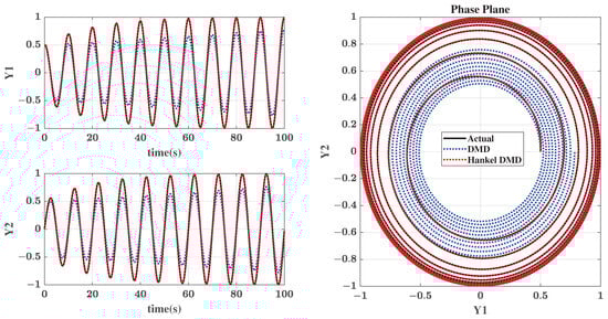
Figure 1.
Nonlinear dynamical system in Equation (47) with no control input and measurement noise: Actual trajectory and trajectories reconstructed from Dynamic Mode Decomposition (DMD) and Hankel Dynamic Mode Decomposition (Hankel DMD) models.
Next, the system in Equation (47) is simulated with initial condition and a doublet control input at s and another at s. No measurement noise is added in this case. The data are split into training and test data using a single split at s. The training data are used for the estimation of the HDMDc model. Figure 2 shows the actual output trajectory as well as that reconstructed from the HDMDc model using the same initial condition and control inputs. To demonstrate the effectiveness of the model, the normalized root mean square error (NRMSE) and FIT% of the reconstructed trajectory with both the training and test data are computed. Throughout this paper, the range-based NRMSE is used. That is, the root mean square error (RMSE) is normalized by the difference between the maximum and the minimum values to obtain NRMSE. The FIT% is computed as , where is the RMSE computed for the data with respect to the mean of the data. The model is able to fit the training data with an NRMSE of 0.0027 and the test data with 0.0064. The training and test FIT% achieved are 98.4 and 96.7, respectively.
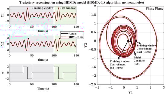
Figure 2.
Nonlinear dynamical system in Equation (47) with control input but no measurement noise: Actual trajectory and the trajectory reconstructed from Hankel Dynamic Mode Decomposition with Control (HDMDc) model estimated using HDMDc-LS (standard algorithm using least squares approach).
To capture the dynamics in this case, d is taken as 300 (299 delays are used to augment outputs), ℓ is taken as 60 (SVD truncation of ), and s is taken as 6 (model reduction) to obtain a reduced-order Hankel DMDc model. The d value is chosen by trial and error. For the chosen d, initial values of ℓ and s are obtained based on singular value plots as shown in Figure 3 and finalized using the trial and error method. The initial values of ℓ and s are chosen as the singular index value after which the curves flatten off. Starting at this initial guess, the trial and error method is employed to obtain a better fit of the model-generated trajectory with the test data. The final values of ℓ and s used are also indicated in Figure 3. As seen from the figure, the final values are close to the initial guesses (values at which the curves flatten).
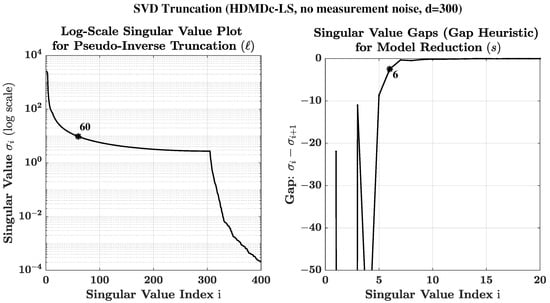
Figure 3.
Nonlinear dynamical system in Equation (47) with control input but no measurement noise: Singular values plot and singular value gap plot to enable the selection of the parameter values for model estimation using HDMDc-LS (standard algorithm using least squares approach). Symbol * in the plots above indicates the final chosen values used to produce the results in Figure 2.
Table 1 presents the sensitivity analysis, that is, the effect of variation of the model parameters d, ℓ, and s on the model fit obtained. Root mean square error (RMSE), NRMSE, and FIT% of the reconstructed trajectory with both the training and test data are presented for various values of the parameters. The cell backgrounds are color-coded, with the green color indicating a better model fit than the red color. The table only shows these values for the reconstructed signal. The reconstructed signal shows the same trend. From the table, it is clear that the chosen parameter values are near-optimal. Further increase in d, ℓ, and s does not improve the model fit much. The values of d, ℓ, and s used to produce the results in Figure 2 are highlighted in bold in the table.

Table 1.
Nonlinear dynamical system in Equation (47) with control input but no measurement noise: Sensitivity analysis of parameters for HDMDc-LS.
Although HDMDc-LS, based on the ordinary least squares approach, performed well in capturing the dynamics in the case with no noise, it is expected not to provide a consistent estimate of the system matrices in the case where the input measurement has noise. In this regard, the next simulation considers equal noise added to all the outputs and the control input. The simulation uses and . Figure 4 shows the measured output trajectory. The standard Hankel DMDc algorithm (HDMDc-LS), as well as the proposed HDMDc with total least squares algorithm, are used to estimate the system matrices. The number of output delays used to augment the output is kept the same as before. For the standard HDMDc algorithm (HDMDc-LS), ℓ is taken as 70 (SVD truncation of ) and s is taken as 45 (the same model reduction order as in HDMDc-TLS discussed below) to obtain a reduced-order Hankel DMDc model. The parameter ℓ is chosen as discussed for the no-noise case. Note that the SVD truncation of the matrix also serves as a noise filtering mechanism, and therefore the truncation rank used is case-specific depending on the measurement noise. The selection procedure, as described before, is by trial and error, guided by the singular value plots. As seen from Figure 4, the reconstructed trajectory from the Hankel DMDc model estimated using the HDMDc-LS does not closely follow the actual one. A quantification of the model fit obtained is given in Table 2. The deviations are substantial in the duration when the control input is applied.
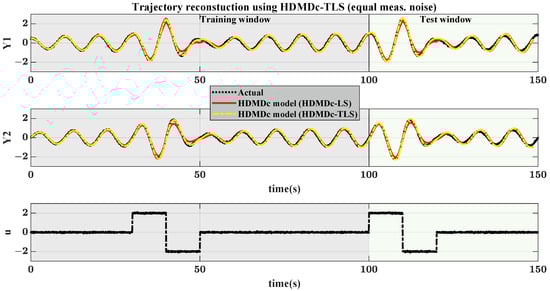
Figure 4.
Nonlinear dynamical system in Equation (47) with equal measurement noise in control and outputs: Actual trajectory and the trajectories reconstructed from the HDMDc models obtained using HDMDc-LS and HDMDc-TLS (total least squares approach) algorithms.
Table 2.
Nonlinear dynamical system in Equation (47) with equal measurement noise in control and outputs: Quantification of the model fit for HDMDc-LS.
Figure 4 also shows the reconstructed output trajectory obtained from the Hankel DMDc model estimated using the HDMDc-TLS algorithm. Since the measurement noise characteristics are equal for all outputs and the input, the reconstructed trajectory matches the original trajectory. Even though the reconstructed trajectory matches well with the actual one, a small time shift is observed toward the end. The model fit, quantified in terms of RMSE, NRMSE, and FIT%, is shown in Table 3. The table shows the sensitivity of the model fit to the truncation values used. For HDMDc-TLS, is taken as 45 (SVD truncation of ) and s is taken as 45 (model reduction) to obtain a reduced-order model. The parameter is chosen guided by the singular value plot as shown in Figure 5. The model order s is kept the same as . The order of the reduced-order model cannot be greater than as is constructed using the truncated SVD using Equation (29). From Table 3, it is seen that the chosen of 45 is near optimum. The model fit for both training and test data is maximum for . The HDMDc-TLS model matches the test data with an NRMSE of 0.0329 for (used in simulation) against the value of 0.0437 for the model estimated using HDMDc-LS for the signal.
Table 3.
Nonlinear dynamical system in Equation (47) with equal measurement noise in control and outputs: Sensitivity analysis of parameters for HDMDc-TLS.
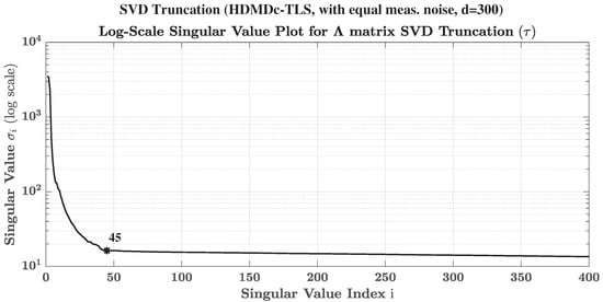
Figure 5.
Nonlinear dynamical system in Equation (47) with equal measurement noise in control and outputs: Singular values plot for estimating model using HDMDc-TLS (algorithm using total least squares approach). Symbol * in the plot above indicates the final chosen value used to produce the results in Figure 4.
Table 4 shows the confidence bounds () of the system eigenvalues obtained using Monte-Carlo simulations (200 simulations). Eigenvalues corresponding to the first two dominant modes are shown in the table. The values estimated using both HDMDc-LS and HDMDc-TLS algorithms are included. Eigenvalues estimated using HDMD corresponding to the noise-free case (without control input) are also presented for reference. The first mode corresponds to the limit cycle oscillation, and the second mode is the damping mode. The mean of the estimated system eigenvalues using HDMDc-TLS is closer to the reference value than that obtained using HDMDc-LS, indicating lower bias in the HDMDc-TLS-based estimates. Additionally, the confidence bounds (reflecting variability across noise realizations) are smaller for HDMDc-TLS.
Table 4.
Nonlinear dynamical system in Equation (47) with equal measurement noise in control and outputs: Estimated system eigenvalues with confidence bounds—HDMDc-TLS.
Next, the system in Equation (47) is simulated with unequal noise added to all the outputs and the control inputs. In particular, and . Figure 6 shows the actual trajectory (measured with noise) and the reconstructed output trajectories obtained using the Hankel DMDc model, estimated using HDMDc-BELS and HDMDc-LS algorithms. The plant model estimated using the proposed HDMDc-BELS algorithm, which is designed to handle unequal noises in measurements, is able to reconstruct trajectories from the initial conditions that match the actual trajectory. For HDMDc-LS, ℓ is taken as 35 (SVD truncation of ) and for HDMDc-BELS, ℓ is taken as 35 (SVD truncation of ). For both algorithms, s is taken as 6 (order of the reduced-order model) to obtain reduced-order models. The number of output delays used to augment the output is kept the same for comparison purposes. The initial values of ℓ and s for the HDMDc-BELS algorithm are chosen based on singular value plots as shown in Figure 7 and finalized using the trial and error method. Table 5 shows the sensitivity of the model fit to parameter variations. The chosen value of 35 for ℓ is near optimum. The model fit for both training and test data is maximum for . The model is able to fit the signal of training data with an NRMSE of 0.0356 and test data with 0.0424 for . The training and test FIT% achieved are about 77.5 and 77.0, respectively. Although the FIT% values appear less in the absolute sense, it has to be compared relative to the model fit achieved in the case of HDMDc-LS, where the prediction diverged from the ground truth.
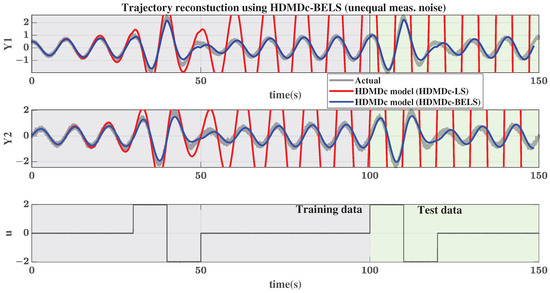
Figure 6.
Nonlinear dynamical system in Equation (47) with unequal measurement noise in control and outputs: Actual trajectory and the trajectories reconstructed from the HDMDc models obtained using HDMDc-LS and HDMDc-BELS (bias eliminating least squares approach) algorithms.
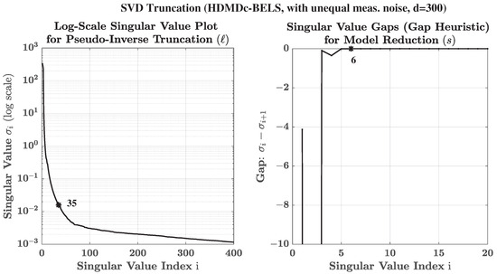
Figure 7.
Nonlinear dynamical system in Equation (47) with equal measurement noise in control and outputs: Singular values plot for estimating model using HDMDc-BELS (algorithm using bias eliminating least squares approach). Symbol * in the plots above indicates the final chosen values used to produce the results in Figure 6.
Table 5.
Nonlinear dynamical system in Equation (47) with equal measurement noise in control and outputs: Sensitivity analysis of parameters for HDMDc-BELS.
Table 6 shows the confidence bounds () of the system eigenvalues obtained using Monte-Carlo simulations (200 simulations) corresponding to the HDMDc-BELS algorithm. Again, eigenvalues corresponding to the first two dominant modes are only shown. The values estimated using both HDMDc-BELS and HDMDc-LS algorithms are included. The mean of the system eigenvalues estimated through HDMDc-BELS is closer to the reference value than the one obtained using HDMDc-LS, as expected. The confidence bounds are also smaller for the estimates obtained from HDMDc-BELS.
Table 6.
Nonlinear dynamical system in Equation (47) with equal measurement noise in control and outputs: Estimated system eigenvalues with confidence bounds—HDMDc-BELS (, , ).
Table 7 presents the results of the robustness analysis carried out for the HDMDc-BELS algorithm. Recall that the HDMDc-BELS algorithm requires the knowledge of the noise statistics of the measurements. In this robustness study, the standard deviations of the noise assumed by the estimation algorithm differ from the actual standard deviation of the measurement data. The difference varies up to 10% for the output signals and up to 100% for the control input signal. The variation considered for the control input signal is large, as the nominal noise in the input channel is very small compared to that in the output signals. For the nonlinear example problem, as seen from Table 7, the model fit is robust for up to a 5% difference in the assumed standard deviations of the output sensors. However, there is a notable performance degradation in the model fit if the assumed standard deviation of noise in the output channels (especially ) has about 10% variation from the true noise characteristics. To prevent skewing the results, outliers were removed using the Z-score method before calculating the mean NRMSE. Between 1 and 9 outliers were excluded, depending on the data distribution. In the case of aircraft output sensors, frequent mandatory maintenance calibrations of the sensors ensure that their noise statistics are known accurately. Note that some of the entries in Table 7 are negative. It means that there is a performance improvement when a non-correct value is assumed for the standard deviation of the noise. However, these negative values are small in magnitude, which again illustrates the robustness of the algorithm to error in assumed standard deviation values.
Table 7.
Nonlinear dynamical system in Equation (47) with equal measurement noise in control and outputs: Robustness analysis of HDMDc-BELS (, , ) with respect to error in assumed noise standard deviation.
4.2. Aircraft Steady Spin
Hankel DMDc is now applied to model an aircraft’s steady spin motion. The aircraft model used is T-2, a 5.5% dynamically scaled version of a generic transport aircraft [34]. A MATLAB R2018b® Simulink model of the same is available on GitHub (Simulink model available in https://github.com/nasa/GTM_DesignSim, accessed on 25 July 2025, released by NASA). The Simulink model was saved in R2018a format for compatibility with the laptop’s MATLAB installation (HP ProBook x360 440 G1, Intel(R) Core(TM) i7-8550U, 8 GB RAM; HP Inc., Palo Alto, CA, USA) and used for data generation. The aerodynamic database of the model is in the form of multidimensional tables.
Here, the measurements available are aircraft angle of attack , side-slip angle , body axis pitch rate q, roll rate p, yaw rate r, longitudinal acceleration , lateral acceleration , and vertical acceleration . The controls are elevator deflection , aileron deflection , and rudder deflection . That is,
Measurements are sampled at 200 Hz. A white noise having zero mean following a normal distribution was added to the measurements to simulate measurement noise. Noise characteristics were taken from the NASA T-2 Simulink model. Table 8 shows the measurement noise characteristics used.
Table 8.
Measurement noise (standard deviation of the normal distribution) in various outputs and inputs.
The simulation is started with an approximate spin state as the initial condition. The aircraft then starts entering spin, and the spin becomes stabilized at about 18 s. The noise-free outputs during the steady spin conditions are deg, deg, deg/s, deg/s, and deg/s with control deflections deg, deg, and deg
While the aircraft is in the steady spin, doublet inputs are given to the control surfaces. Doublet input is used regularly in aircraft parameter estimation. The details of the input applied are as follows. At time s, a doublet input of 4 s duration is given to the elevator, aileron, and rudder in succession, separated by 1 s gap (see Figure 8). A doublet input of 2 s duration is again applied at s to the rudder, aileron, and elevator in succession. Note that the order in which the doublet input is applied in succession has changed from (elevator, aileron, rudder) to (rudder, aileron, elevator). Although the control input step is instantaneous, the control surface deflections are not, owing to the actuator model in the Simulink model. The data starting from s are split into training and test data using a single split at s. The training data are used for the estimation of the HDMDc model.
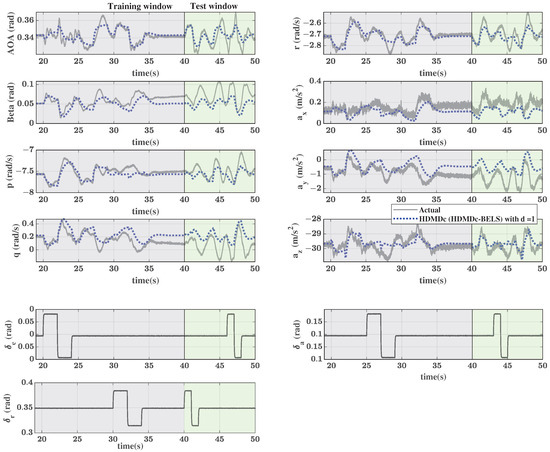
Figure 8.
T-2 RC aircraft steady spin simulation: Trajectory reconstruction using HDMDc model (HDMDc-BELS) for doublet input with .
Figure 8 shows the output time history along with the inputs. The figure also shows the reconstructed trajectory using the Hankel DMDc plant model estimated using the HDMDc-BELS algorithm with no time delay embedding, that is, . For this case, the SVD truncation was not carried out. From the figure, it is clear that the reconstructed trajectory does not match the actual trajectory if there is no time delay embedding of outputs and control inputs. The NRMSE values corresponding to the model fit are 0.158 for the training data and 0.250 for the test data.
Figure 9 shows the reconstructed trajectory using the plant model estimated using the HDMDc-BELS algorithm with . The reconstructed trajectory matches well with the actual one. The NRMSE error values (for the state ) achieved for the training and test data are 0.032 and 0.045, respectively. The fits obtained in the other states have a similar trend and are not reported here for brevity. Notably, the plant model estimated from the training data set was able to capture the spin motion beyond the training period. This is despite the fact that the system was perturbed by a different set of control inputs in the testing period. For the SVD truncation of , ℓ is taken as 37, and s is taken as 24 to obtain the reduced-order model. Again, the values for d, ℓ, and s were arrived at from initial guesses based on singular value plots, which were further refined using trial and error.
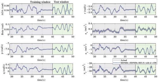
Figure 9.
T-2 RC aircraft steady spin simulation: Trajectory reconstruction using HDMDc model (HDMDc-BELS) for doublet input with (, ).
Table 9 shows the results of the sensitivity analysis carried out. The model fit quantified by NRMSE is compared for various values of d, ℓ, and s. The cell backgrounds of the table are color-coded as before, with green color indicating a better model fit than red color. The data shown in the table correspond to signal. Other signals also show a similar trend. From the table, it is clear that the parameter values chosen for the simulation are near optimum.
Table 9.
T-2 RC aircraft steady spin simulation: Sensitivity analysis of HDMDc-BELS (doublet input).
For reconstructing the trajectory, the full-order HDMDc model required an average of 4.96 s (timed over 10 runs), while the reduced-order model took only 0.11 s. This points to the computational advantage of using reduced-order models, especially in real-time scenarios. The timing was measured using the tic and toc framework in MATLAB(R2018a) on a standard laptop (HP ProBook x360 440 G1, Intel(R) Core(TM) i7-8550U, 8 GB RAM; HP Inc., Palo Alto, CA, USA), without parallelization.
Next, at 20 s, instead of a doublet input, a multisine input (a summation of sine signals of varying frequency, amplitude, and phase) of 10 s duration is applied to all the control surfaces (taken from [3] and scaled). Figure 10 shows the output time history along with the inputs. The figure also shows the trajectory predicted using the Hankel DMDc plant model obtained from the doublet data. To obtain the predicted trajectory, the system matrices gathered from the doublet training data are used along with the multisine input and initial conditions used in this test case. As seen from the figure, the predicted trajectory matches well with the actual one, showing only minor deviations. Table 10 gives the NRMSE values for the fit obtained in all the output channels. This result establishes that the model learned is generic, in the sense that it is robust to changes in the input signal.
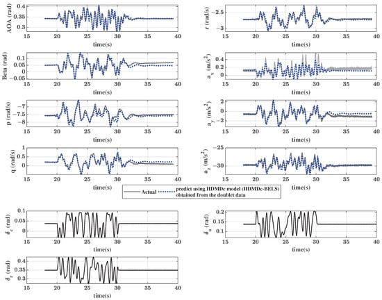
Figure 10.
T-2 RC aircraft steady spin simulation: Trajectory prediction using HDMDc (HDMDc-BELS) for multisine input.
Table 10.
T-2 RC aircraft steady spin simulation: NMRSE for reconstructed and predicted trajectories (, , ).
To further establish the efficacy of the learned model, the model is tested for its predictive capability for a different initial condition. A different initial condition leads the aircraft to a different steady spin state. The simulation details are as follows. The noise-free outputs during the steady spin conditions are deg, deg, deg/s, deg/s, and deg/s with control deflections deg, deg, and deg. Notice the differences in the spin AOA, side-slip angle, roll rate, and rudder deflection compared to the previous simulation. Figure 11 shows the predicted trajectory using the Hankel DMDc plant model obtained from the data for the original spin condition. Although the model used for prediction was estimated from a data set having a different initial condition, the trends of the predicted trajectory are similar to those of the actual trajectory, even though the match is not perfect. The fits obtained for the predicted trajectory in all the output channels are reported in Table 10. The NRMSE values in this case are higher than those for the case in which multisine inputs were used instead of doublets. This indicates that the HDMDc model, for the T-2 aircraft considered, can generalize control inputs more than different rotary configurations. This may be due to the underlying aerodynamic model of the T-2 aircraft, wherein the rotary derivatives dominate the control surface derivatives.
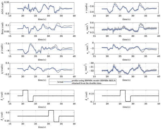
Figure 11.
T-2 RC aircraft steady spin simulation: Trajectory prediction using HDMDc model (HDMDc-BELS) for a different steady spin condition.
4.3. Aircraft Oscillatory Spin
Having demonstrated the effectiveness of Hankel DMDc using the BELS approach for the steady spin case, the Hankel DMDc algorithm is applied to aircraft oscillatory spin data to check whether a faithful plant model can be obtained.
The oscillatory spin of aircraft is numerically simulated using the F-18 HARV model. The aerodynamic coefficients for this aircraft model are available as tables (Aerodynamic data available at https://web.archive.org/web/20170118142930/http://www1.nasa.gov/centers/dryden/history/pastprojects/HARV/Work/NASA2/nasa2.html, accessed on 25 July 2025, released by NASA) [35]. For this system, the outputs and control inputs are
The aircraft is initially trimmed for an angle of attack of 15 deg and a yaw rate of 5 deg/s at an altitude of 12 km. After initializing the simulation with this trim state, a sudden elevator deflection of 24 deg is applied. This causes the aircraft in the simulation to start entering an oscillatory spin, and the spin becomes stabilized (sustained oscillations) at about 40 s. At 70 s, multisine control inputs (taken from [3] and scaled) are applied. The simulation data are recorded by adding noise which has the same characteristics as in the previous case (Table 8).
First, Hankel DMD is applied to data from 40 s to 60 s. This is the duration in which a control input was not applied, and therefore Hankel DMD (without control) suffices to capture the dynamics. Figure 12 shows that the actual trajectory and the trajectory generated from the estimated Hankel DMD model using the same initial conditions match closely. Table 11 shows the NRMSE and FIT% values for all the outputs. The parameter values used in this case are (299 delays are used to augment outputs), (SVD truncation of ) and (model reduction). The delay parameter d is chosen by the trial and error method, and other parameters ℓ and s are chosen initially guided by the singular value plots and later modified using trial and error (as mentioned in Section 4.1 and Section 4.2).
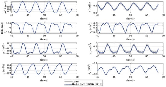
Figure 12.
F-18 oscillatory spin simulation: Trajectory reconstruction using Hankel DMD applied to data from .
Table 11.
F-18 oscillatory spin simulation: NMRSE and FIT% for trajectory reconstruction using Hankel DMD applied to data from (, and ).
Next, Hankel DMDc is applied to the data in the time range of 66 s to 85 s. Recall that the control input spanned 70 to 80 s. Figure 13 shows the actual trajectory and the trajectory reconstructed using the plant model obtained from Hankel DMDc using the same initial conditions and control input. Although the trajectories match well in general, there is a slight difference between the reconstructed trajectory and the actual one in some of the states. This may be due to the fact that the effect of control input is only marginally observed in the outputs other than , , and . Table 12 shows the achieved NRMSE and FIT% values for all the outputs. The NRMSE values are more than double in this case when compared to the no-input case.
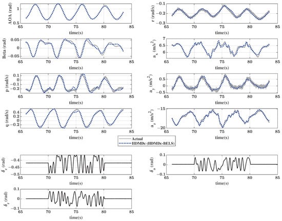
Figure 13.
F-18 oscillatory spin simulation: Trajectory reconstruction using Hankel DMDc applied to data from (, , ).
Table 12.
F-18 oscillatory spin simulation: NMRSE and FIT% for reconstructed trajectory using Hankel DMDc applied to data from (, and ).
To capture the system dynamics in this case, d is taken as 300 (299 delays are used to augment outputs), ℓ is taken as 50 (SVD truncation of ), and s is taken as 30 (model reduction) to obtain a reduced-order Hankel DMDc model (parameters chosen as mentioned in Section 4.1 and Section 4.2). The sensitivity of the fit obtained to the parameters d, ℓ, and s is presented in Table 13. The data shown in the table correspond to the signal. From the table, it is clear that the chosen values of , , and are near optimum.
Table 13.
F-18 oscillatory spin simulation: Sensitivity analysis of HDMDc-BELS.
Timing analysis averaged over 10 runs showed that the trajectory reconstruction using full-order HDMDc takes 17.55 s, whereas the reduced-order counterpart takes only 0.11 s, highlighting the performance benefit of reduced-order modeling. All measurements were performed in MATLAB using the built-in tic/toc functions on a single-threaded setup, with no use of GPU or parallel computing (Intel(R) Core(TM) i7-8550U, 8 GB RAM, MATLAB R2018a).
5. Conclusions
This article proposed the use of a data-driven Hankel Dynamic Mode Decomposition with control (HDMDc) method to arrive at a plant model for aircraft spin motion. This approach offers an alternative to traditional nonlinear aerodynamic force and moment plant models, which are often cumbersome to develop.
The motivation for employing the Hankel DMDc framework stemmed from its ability to capture nonlinear dynamics, such as limit cycle oscillations, which standard DMDc struggles with, for dynamical systems with limited outputs. Since traditional Hankel DMDc, which relies on ordinary least squares, is unsuitable for handling the measurement noise scenarios observed in aircraft measurements, modified Hankel DMDc system identification algorithms based on the error-in-variables (EIV) approach were proposed. In particular, two EIV-based approaches were presented: total least squares and bias eliminating least squares.
The efficacy of the proposed modified algorithms was first demonstrated on a simple dynamical system exhibiting limit cycle oscillation, which was excited with a doublet control input. For the case of equal measurement noises added to all the signals, including input, the total least squares-based modification (HDMDc-TLS) performed better than the traditional HDMDc-LS. The model fits had NRMSE values of 0.0219 and 0.0345 for HDMDc-TLS and HDMDc-LS, respectively. When unequal measurement noises were added to the signals, HDMDc-BELS performed well with an NRMSE value of 0.0356. In contrast, the traditional HDMDc model predicted unstable oscillations instead of a limit cycle oscillation. The case of unequal noise is what HDMDc-BELS was developed for, and it was proven to serve the purpose.
Next, the bias-eliminating least squares (BELS)-based Hankel DMDc algorithm was applied to model both steady spin (using simulated data from the NASA T-2 RC aircraft) and oscillatory spin motions (using NASA F-18 HARV aircraft simulation data). It was shown that the plant model estimated using the proposed approach could capture the complex spin dynamics. For the steady spin of the T-2 aircraft, the estimated model not only accurately regenerated the actual trajectories (NRMSE values of 0.03238 and 0.04827 for the training and test data, respectively, for the angle of attack prediction) but also correctly predicted spin motion even when the initial conditions and control inputs varied from the training data. Notably, the learned model accurately predicted trajectories (model fit with NRMSE value of 0.04872 for angle of attack) even when the control input changed from a doublet in the training data to a multisine input in the testing data. Even for an input different from that used for training, resulting in the aircraft entering a different spin state, a model fit with NRMSE of 0.06455 was obtained in angle of attack channel. Predictions of the other outputs also depicted similar performances. This demonstrates the robustness of the captured model, suggesting its potential for studying and evaluating various techniques for aircraft spin recovery.
Future work will involve validating the proposed EIV-based Hankel DMDc approach using experimental in-flight aircraft spin data. Further, the suitability of the proposed methodology could be investigated for other complex, highly nonlinear aircraft maneuvers.
Author Contributions
Conceptualization, B.S. and J.G.M.; methodology, B.S.; software, B.S.; validation, B.S. and J.G.M.; investigation, B.S.; resources, B.S.; data curation, B.S.; writing—original draft preparation, B.S.; writing—review and editing, J.G.M.; visualization, B.S.; supervision, J.G.M. All authors have read and agreed to the published version of the manuscript.
Funding
This research received no external funding.
Data Availability Statement
No new data were created or analyzed in this study. The algorithm used is fully described in the article, and the simulation data were generated using publicly available datasets or models, as cited. The computer code used to produce the results is available from the corresponding author upon reasonable request.
Acknowledgments
The first author thanks Shanker Narashimhan, Indian Institute of Technology, Madras, for his suggestions regarding EIV approaches. The second author acknowledges the support he received from Geophysical Flows Lab, IIT Madras.
Conflicts of Interest
The authors declare no conflicts of interest.
Abbreviations
The following abbreviations are used in this manuscript:
| DMD | Dynamic Mode Decomposition |
| DMDc | Dynamic Mode Decomposition With Control |
| HDMDc | Hankel Dynamic Mode Decomposition With Control |
| EIV | Error-In-Variables |
| LS | Least Squares |
| TLS | Total Least Squares |
| BELS | Bias-Eliminating Least Squares |
| SVD | Singular Value Decomposition |
| AOA | Angle of Attack |
| NASA | National Aeronautics and Space Administration |
| RMSE | Root Mean Square Error |
| NRMSE | Normalized Root Mean Square Error |
| FIT% | Goodness-of-Fit Percentage |
References
- Day, R.E. Coupling Dynamics in Aircraft: A Historical Perspective; National Aeronautics and Space Administration: Washington, DC, USA, 1997; Volume 532. [Google Scholar]
- Farcy, D.; Khrabrov, A.N.; Sidoryuk, M.E. Sensitivity of Spin Parameters to Uncertainties of the Aircraft Aerodynamic Model. J. Aircr. 2020, 57, 922–937. [Google Scholar] [CrossRef]
- Gresham, J.L.; Simmons, B.M.; Hopwood, J.W.; Woolsey, C.A. Spin Aerodynamic Modeling for a Fixed-Wing Aircraft Using Flight Data. J. Aircr. 2024, 61, 128–139. [Google Scholar] [CrossRef]
- Morelli, E.A. Global nonlinear aerodynamic modeling using multivariate orthogonal functions. J. Aircr. 1995, 32, 270–277. [Google Scholar] [CrossRef]
- Mokhtari, M.; Sabzehparvar, M. Identification of spin maneuver aerodynamic nonlinear model by applying ensemble empirical mode decomposition and extended multipoint modeling. Proc. Inst. Mech. Eng. Part G J. Aerosp. Eng. 2019, 233, 1865–1878. [Google Scholar] [CrossRef]
- Proctor, J.L.; Brunton, S.L.; Kutz, J.N. Dynamic Mode Decomposition with Control. SIAM J. Appl. Dyn. Syst. 2016, 15, 142–161. [Google Scholar] [CrossRef]
- Nedzhibov, G. An Improved Approach for Implementing Dynamic Mode Decomposition with Control. Computation 2023, 11, 201. [Google Scholar] [CrossRef]
- Volchko, A.; Mitchell, S.K.; Morrissey, T.G.; Humbert, J.S. Model-based data-driven system identification and controller synthesis framework for precise control of SISO and MISO HASEL-powered robotic systems. In Proceedings of the 2022 IEEE 5th International Conference on Soft Robotics (RoboSoft), Edinburgh, Scotland, 4–8 April 2022; pp. 209–216. [Google Scholar]
- Fonzi, N.; Brunton, S.L.; Fasel, U. Data-driven nonlinear aeroelastic models of morphing wings for control. Proc. R. Soc. A 2020, 476, 20200079. [Google Scholar] [CrossRef]
- Tu, J.H.; Rowley, C.W.; Luchtenburg, D.M.; Brunton, S.L.; Kutz, J.N. On dynamic mode decomposition: Theory and applications. J. Comput. Dyn. 2014, 1, 391–421. [Google Scholar] [CrossRef]
- Brunton, S.L.; Budišić, M.; Kaiser, E.; Kutz, J.N. Modern Koopman Theory for Dynamical Systems. SIAM Rev. 2022, 64. [Google Scholar] [CrossRef]
- Kang, W.; Hu, S.; Chen, B.; Yao, W. Modal Phase Study on Lift Enhancement of a Locally Flexible Membrane Airfoil Using Dynamic Mode Decomposition. Aerospace 2025, 12, 313. [Google Scholar] [CrossRef]
- Luo, X.; Kareem, A. Dynamic mode decomposition of random pressure fields over bluff bodies. J. Eng. Mech. 2021, 147, 04021007. [Google Scholar] [CrossRef]
- Barocio, E.; Pal, B.C.; Thornhill, N.F.; Messina, A.R. A Dynamic Mode Decomposition Framework for Global Power System Oscillation Analysis. IEEE Trans. Power Syst. 2015, 30, 2902–2912. [Google Scholar] [CrossRef]
- Mezić, I. Spectral properties of dynamical systems, model reduction and decompositions. Nonlinear Dyn. 2005, 41, 309–325. [Google Scholar] [CrossRef]
- Rowley, C.W.; Mezić, I.; Bagheri, S.; Schlatter, P.; Henningson, D.S. Spectral analysis of nonlinear flows. J. Fluid Mech. 2009, 641, 115–127. [Google Scholar] [CrossRef]
- Colbrook, M.J. The multiverse of dynamic mode decomposition algorithms. In Handbook of Numerical Analysis; Elsevier: Amsterdam, The Netherlands, 2024; Volume 25, pp. 127–230. [Google Scholar]
- Williams, M.O.; Kevrekidis, I.G.; Rowley, C.W. A data–driven approximation of the koopman operator: Extending dynamic mode decomposition. J. Nonlinear Sci. 2015, 25, 1307–1346. [Google Scholar] [CrossRef]
- Arbabi, H.; Mezic, I. Ergodic theory, dynamic mode decomposition, and computation of spectral properties of the Koopman operator. SIAM J. Appl. Dyn. Syst. 2017, 16, 2096–2126. [Google Scholar] [CrossRef]
- Le Clainche, S.; Vega, J.M. Higher order dynamic mode decomposition. SIAM J. Appl. Dyn. Syst. 2017, 16, 882–925. [Google Scholar] [CrossRef]
- Patanè, L.; Sapuppo, F.; Xibilia, M.G. Soft Sensors for Industrial Processes Using Multi-Step-Ahead Hankel Dynamic Mode Decomposition with Control. Electronics 2024, 13, 3047. [Google Scholar] [CrossRef]
- Ling, E.; Ratliff, L.; Coogan, S. Koopman operator approach for instability detection and mitigation in signalized traffic. In Proceedings of the 2018 21st International Conference on Intelligent Transportation Systems (ITSC), IEEE, Maui, HI, USA, 4–7 November 2018; pp. 1297–1302. [Google Scholar]
- Mustavee, S.; Agarwal, S.; Enyioha, C.; Das, S. A linear dynamical perspective on epidemiology: Interplay between early COVID-19 outbreak and human mobility. Nonlinear Dyn. 2022, 109, 1233–1252. [Google Scholar] [CrossRef] [PubMed]
- Deiler, C.; Mönnich, W.; Seher-Weiss, S.; Wartmann, J. Retrospective and Recent Examples of Aircraft and Rotorcraft System Identification at DLR. J. Aircr. 2023, 60, 1371–1397. [Google Scholar] [CrossRef]
- Chen, R.T.; Rubanova, Y.; Bettencourt, J.; Duvenaud, D.K. Neural ordinary differential equations. In Proceedings of the Advances in Neural Information Processing Systems 31 (NeurIPS 2018), Montreal, QC, Canada, 3–8 December 2018; Volume 31. [Google Scholar]
- Hochreiter, S.; Schmidhuber, J. Long short-term memory. Neural Comput. 1997, 9, 1735–1780. [Google Scholar] [CrossRef]
- Wang, Y. A new concept using LSTM Neural Networks for dynamic system identification. In Proceedings of the 2017 American Control Conference (ACC), Seattle, WA, USA, 24–26 May 2017; pp. 5324–5329. [Google Scholar]
- Dawson, S.T.M.; Hemati, M.S.; Williams, M.O.; Rowley, C.W. Characterizing and correcting for the effect of sensor noise in the dynamic mode decomposition. Exp. Fluids 2016, 57, 42. [Google Scholar] [CrossRef]
- Hemati, M.S.; Rowley, C.W.; Deem, E.A.; Cattafesta, L.N. De-biasing the dynamic mode decomposition for applied Koopman spectral analysis of noisy datasets. Theor. Comput. Fluid Dyn. 2017, 31, 349–368. [Google Scholar] [CrossRef]
- Söderström, T. Errors-in-Variables Methods in System Identification; Communications and Control Engineering; Springer International Publishing: Berlin/Heidelberg, Germany, 2018. [Google Scholar]
- Meng, Q.; Kasis, A.; Yang, H.; Polycarpou, M.M. Secure state estimation of networked switched systems under denial-of-service attacks. Eur. J. Control 2024, 80, 101037. [Google Scholar] [CrossRef]
- Van Huffel, S.; Zha, H. The total least squares problem. In Handbook of Statistics; Computational Statistics; Elsevier: Amsterdam, The Netherlands, 1993; Volume 9, pp. 377–408. [Google Scholar]
- James, P.; Souter, P.; Dixon, D. Suboptimal estimation of the parameters of discrete systems in the presence of correlated noise. Electron. Lett. 1972, 8, 411–412. [Google Scholar] [CrossRef]
- Jordan, T.; Bailey, R. NASA Langley’s AirSTAR Testbed: A Subscale Flight Test Capability for Flight Dynamics and Control System Experiments. In Proceedings of the AIAA Guidance, Navigation and Control Conference and Exhibit, AIAA, Honolulu, HI, USA, 18–21 August 2008. [Google Scholar]
- Sinha, N.K.; Ananthkrishnan, N. Advanced Flight Dynamics with Elements of Flight Control; CRC Press: Boca Raton, FL, USA, 2017. [Google Scholar]
Disclaimer/Publisher’s Note: The statements, opinions and data contained in all publications are solely those of the individual author(s) and contributor(s) and not of MDPI and/or the editor(s). MDPI and/or the editor(s) disclaim responsibility for any injury to people or property resulting from any ideas, methods, instructions or products referred to in the content. |
© 2025 by the authors. Licensee MDPI, Basel, Switzerland. This article is an open access article distributed under the terms and conditions of the Creative Commons Attribution (CC BY) license (https://creativecommons.org/licenses/by/4.0/).