Article

A Framework for an ML-Based Predictive Turbofan Engine Health Model

1
Department of Mechanical Engineering, Virginia Polytechnic Institute and State University, Blacksburg, VA 24061, USA
2
Rolls-Royce plc, London N1 9FX, UK
*
Author to whom correspondence should be addressed.
Aerospace 2025, 12(8), 725; https://doi.org/10.3390/aerospace12080725
Submission received: 4 June 2025 / Revised: 7 August 2025 / Accepted: 11 August 2025 / Published: 14 August 2025
(This article belongs to the Section Aeronautics)

Abstract

A predictive health modeling framework was developed for a family of turbofan engines, focusing on early detection of performance degradation. Turbine Gas Temperature (TGT) was employed as the primary indicator of engine health within the model, due to its strong correlation with core engine performance and thermal stress. The present research uses engine health monitoring (EHM) data acquired from in-service turbofan family engines. TGT is typically measured downstream of the high-pressure turbine stage and is regarded as the key thermodynamic variable of the gas turbine cycle. Three new training approaches were proposed using data segmentation based on time between major overhauls and compared with the conventional train–test split method. Detrending was employed to effectively remove trends and seasonality, enabling the ML-based model to learn more intrinsic relationships. Large generalized models based on the entire engine family were also investigated. Prediction performance was evaluated using selected machine learning (ML) models, including both linear and nonlinear algorithms, as well as a long short-term memory (LSTM) approach. The models were compared based on accuracy and other relevant performance metrics. The prediction accuracies of ML models depend on the selection of data size and segmentation for training and testing. For individual engines, the proposed training approaches predicted TGT with the accuracy of 4 C to 6 C in root mean square error (RMSE) by utilizing 65% less data than the train (80%)–test (20%) split method. Utilizing the data of each family engine, the large generalized model achieved similar prediction accuracy in RMSE with a smaller interquartile range. However, the amount of data required was 45–300 times larger than the proposed approaches. The sensitivity of prediction accuracy to the size of the training dataset offers valuable insights into the framework’s applicability, even for engines with limited data availability. Uncertainty quantification showed a coverage width criterion (CWC) between 29 C and 40 C, varying with different family engines.

1. Introduction

The safe and economic operation of aircraft engine is crucial for the sustainability of modern life and industry. Hence, the forecasting capability of engine deterioration can provide great value in supporting performance assessment and optimizing maintenance plans. The original equipment manufacturers monitor in-service engines worldwide to ensure their serviceability and operational safety through engine health monitoring (EHM) system. Though idealized physics-based models can be built, producing faithful predictions is still challenging, as individual engines operate under a wide variety of conditions and experience different flight cycles.
These considerations motivate the adoption of machine learning (ML) models that leverage available EHM data from in-service engines. The authors also would like to acknowledge that data-driven approaches to engine prognostics have been adopted by many researchers. A survey on data-driven models and artificial intelligence (AI) for prognostics showed that AI and ML techniques, alongside physics-based approaches, could contribute to building an effective prognostic system [1,2].
Figure 1 shows previous works in the prognostics of gas turbine engines from 62 research papers over the past 20 years. The survey was based on four categories: (a) model, (b) type of gas turbine, (c) source of data, and (d) target variables. It is worth noting that many previous works employed an ML approach to build prognostics models, while there have only been a few of them using physics-based engine performance models (Figure 1a).
Saxena et al. (2008) addressed the challenge posed by the lack of run-to-failure datasets for data-driven prognostics by proposing a method to model damage propagation within aircraft gas turbine engine modules [3]. Li (2010) introduced a novel adaptive gas path analysis (adaptive GPA) approach developed to estimate engine performance and gas path component health status using gas path measurements [4]. Pinelli et al. (2012) presented a comprehensive approach for the measurement validation and health state assessment of gas turbines through gas path analysis (GPA) techniques. These approaches were utilized to calculate machine health state indices from field measurements to support on-condition maintenance [5]. Alozie et al. (2019) presented an adaptive framework for prognostics in civil aero gas turbine engines, aiming to predict the remaining useful life of components by incorporating both performance and degradation models [6]. Fang et al. (2020) carried out a multi-attribute comprehensive evaluation of gas turbine health status combined with a 2000 h test [7].
The remarkable potential of deep learning in processing vast datasets was underscored in a special issue of Nature in 2015 [8], leading to a surge in the popularity of data-driven approaches thereafter. Various types of neural networks were employed, including artificial neural networks (ANNs), deep neural networks (DNNs), convolutional neural networks (CNNs), recurrent neural networks (RNNs), etc. It is worth highlighting that RNN-based models most frequently utilized long short-term memory (LSTM).
Long short-term memory (LSTM) has been found in many previous works using ML to build engine prognostic models (Figure 1a). LSTM is a variant of recurrent neural networks (RNNs) proposed by Hochreiter et al. [9]. It alleviates the vanishing gradient and exploding gradient problems of traditional RNNs, enabling it to handle long-term dependencies in sequence data. A key characteristic of aero engine data is its nature as multivariate time series, which has contributed to the widespread adoption of LSTM models in prior research.
It was found that most researchers had to use their own simulated data or the NASA Commercial Modular Aero-Propulsion System Simulation (C-MAPSS) dataset, as described in Table 1 and Figure 1c. The dataset, based on simulated engine data specifically for turbofan engines with 90,000 lb thrust [10], was first introduced at the 1st International Conference on Prognostics and Health Management (PHM08) [3], and it has been available to the public since 2016 [11]. It has become widely used to build and test predictive models for remaining useful life (RUL) prediction. Consequently, most research has been conducted on gas turbines for aero application (Aero); the most common target variable is RUL (Figure 1b,c).
Referring to Figure 1c, only 17.7% of the previous work was based on real engine data, e.g., in-service engine data, measuring engine test data. Marinai, 2004 [12] utilized both simulated data and real in-flight data from the Rolls-Royce Trent 800 engine. Spieler et al., 2009 [13] used engine performance test data together with maintenance record and environmental data for the Rolls-Royce BR710. EHM data was found in several studies from a whole fleet [14] or sampled based on operators and regions [15]. Sometimes, EHM data was used with geographical information collected from regional airlines [16]. Utilization of both synthetic data and engine data was also found in several studies for model validation [17,18].
Figure 1d illustrates the target variables that were used in previous research: RUL, TGT (or EGT), health state, and engine performance. Due to the availability of the NASA C-MAPSS dataset, the majority of previous research focused on RUL prediction.
A significant portion of previous research—82.3%—relied on simulated data. These studies primarily focused on comparing the benchmarks of different ML algorithms instead of addressing the operating conditions of in-service engines. Moreover, the data was limited to a single engine and covered only a relatively short period.
However, building a prognostics model using simulated data can be of limited efficacy, as such data are typically complete, clean, and structured to include all information necessary for model development. For instance, the NASA C-MAPSS dataset incorporated health parameters and clearly indicated RUL degradation. On the other hand, in-service engine data would come as incomplete and unclean, e.g., lost data and noise, requiring comprehensive data observation and preprocessing before utilizing it.
Table 1. Predictor variables for engine prognostics from literature survey (Note: See Table A1 in Appendix A for references that used NASA C-MAPSS dataset; NASA C-MAPSS dataset variables are available in [3,10,11].
ReferencesList of Predictor VariablesNo. Var.ModelGT TypeTarget
[19] m in , air , p in , air , T in , air , x in , air , m in , water , T in , water , p out , air , T out , air , T out , water , Δ m out , water 10MLindustrialperformance
[20]load, T amb , relative humidity3MLindustrialperformance
[4] T amb , P amb , A nozzle , T 3 , P 3 , T 7 , P 7 , FF, N9physics-basedaerohealth state
[5] T 1 , T 2 , P 2 , P amb , T 3 , T 6 , T 7 , RH, Δ P filter , VAR, N GGT , N PT , P out 13physics-basedindustrialhealth state
[21] T comp , T turb , P comp , P turb , N, FF6MLaeroTGT
[22]n/a (not given)14MLaeroTGT margin
[23]n/a (not given)10MLaeroTGT margin
[24]damage index, starts, trips, vendor type, ρ dust , PM 2.5 , ρ dust , ρ sea   salt , PM 2.5 , ρ sea   salt , ACC1, ACC2, ρ organic   carbon , ρ black   carbon 12MLindustrialRUL
[25]N1, N 2 , P 22 , P 3 , P 5 , T 44 6MLaerofault classes
[26] T 24 , T 50 , P 30 , N 1 , P s 30 , Phi, N 2 corr 7MLaeroRUL
[27] N 1 , N 2 , Pitch, AOA, Roll, Vertical   Acc . , TAT, Ground/Air8MLaeroperformance
[28]ALT, MN, FF, Power4MLaeroperformance
[7] T amb , P amb , P 2 , P 3 , P 6 , T 6 , T 7 , N 1 , N 2 , FF, . . . 10+physics-basedmarinehealth state
[29] T 25 , P 25 , T 3 , P 3 , FF, N 1 , N 2 , N 3 , T 43 , P 43 , T 46 , P 46 , T 5 , P 5 14MLaeroperformance
[30]SLOAT, ALT, T 2 A , MN, N 1 , N 2 6MLaeroEGT margin
[31] T 2 , P 2 , N comp , N fan , T fan , P 3 , P fan , T fuel , T oil , Δ P fuel   filter , Fuel Feeding, Nozzle Throat, Throttle position13MLaeroEGT
[32] N 1 , P 3 , P 34 , T 34 , Q m f 5MLaeroRUL, EOH
[33]shape parameter, EngCycRem, TCI, InspInterval, CycOneTimeInsp, InspModel, ReplaceAll7MLaeromaintenance optimization
NASA C-MAPSS Studies (see Table A1 in Appendix A)NASA C-MAPSS dataset7–46ML/physics-basedaeroRUL
To summarize, the aforementioned findings provide valuable insights that inform the development of the engine predictive model proposed in this study. These insights include: (1) trends in engine prognostics; (2) the impact and difficulty of utilizing in-service real engine data; and (3) the value of building predictive models that can be expanded to multiple and various fleets of engines, not limited to a single engine.
The authors are granted access to the EHM data of three different turbofan family engines encompassing several hundreds of engines, installed on civil aircraft, spanning up to 20 years. The present research includes data observation, preprocessing, and key predictor variable selection. Detrending, another data preprocessing technique, is also introduced in this paper. In addition, this study proposes novel data segmentation approaches based on time intervals between major overhauls of individual engines.
This paper presents an analysis of the accuracy and outlier behavior of ML-based predictive engine health models, applying LSTM with selected linear and nonlinear regression algorithms to individual engines. In addition, multi-engine-based large generalized models were also developed for each turbofan family engine. The authors would like to highlight the considerable differences in the size of data required for the proposed approach and the large generalized model. Uncertainty quantification was conducted with large models using the ‘Delta’ method. Finally, conclusions and future research are discussed.

2. Preprocessing: Selection of Predictor Variable and Data Segmentation

2.1. EHM Data and Turbine Gas Temperature

Engine health monitoring (EHM) data is a snapshot of data collected from in-service engines under specific flight conditions such as taxi-out, take-off, climb, cruise, and taxi-in. EHM systems offer the capability to monitor engine control parameters and performance. Typical EHM data is a discrete and is limited by the number of installed sensors. Yet, such data is considered valuable, as it allows for observation of long-term engine performance changes. In the present paper, the EHM data from three different turbofan family engines—A, B, and C—were used, each containing data from several hundred engines (Table 2). These engines have high bypass ratios for large civil aircraft.
The high-pressure turbine of a turbofan engine is particularly vulnerable, as it is exposed to extreme temperatures and pressures—potentially as high as 2000 K and 50 bar during a take-off. These conditions impose significant thermal stress on turbine components during every flight cycle. Consequently, thermal fatigue is a problem, and extreme cases can lead to turbine component failure. Monitoring of the turbine gas temperature (TGT) signal at the inlet of the low-pressure turbine allows the health (i.e., life) status of the gas turbine engine to be assessed. Accordingly, TGT was selected as the primary target variable for evaluating engine health. Our model only focuses on predicting TGT during take-off, where the impact of degradation is more significant than other flight conditions during the engine’s mission profile.

2.2. Selection of Predictor Variable

Table 1 presents a compilation of predictor variables employed in engine prognostic models, as documented in the literature. Predominantly, research on aero engines has utilized the NASA C-MAPSS dataset. The dataset contains 26 variables from engine simulations, with the first column denoting the engine unit, the second column indicating the current cycle number, columns 3–5 representing the operational conditions, and columns 6–26 encapsulating 21 sensor data points [3,10,11].
Some studies used in-service engine or flight data to construct prognostic models: data recorded from takeoff to landing [27], Rolls-Royce aero engine Avon-300 [4], Rolls-Royce Trent 800 [12], engine performance test data of Rolls-Royce BR710 [13], Rolls-Royce engine EHM data [14,15], two-shaft stationary gas turbine engine LM2500 [29], and the F100-PW-100 engine [28].
From the literature survey, it was found that previous studies utilized provided or accessible variables to the fullest extent when building prognostic models. Consequently, there was a lack of a variable selection process.
The EHM system conveys more than several hundred parameters; hence, conducting data preprocessing and variable selection is inevitable. Principal component analysis (PCA) [34,35] and the Pearson covariance coefficient [36] can be used to analyze the relationship between each predictor variable and the target variable.
Prior to conducting PCA and calculating Pearson covariance coefficients, EHM parameters exhibiting inter-dependencies, duplications, post-processed values, or non-numeric attributes were systemically excluded. Then, the remaining EHM parameters underwent a comprehensive review. Variables were chosen based on their coefficients, derived from the two aforementioned methods. Variables with Pearson coefficients exceeding 0.6 were initially selected for further analysis.
Table 3 presents the selected groups of the predictor variables and different sets of their combinations. To select the best predictor variables for the ML model predicting TGT, each set of predictor variables was tested (Table 4). Additionally, their availability across different family engines was considered.

2.3. Segmentation of Data Using Engine Maintenance Interval

This section introduces and describes a new data segmentation method for model training based on engine maintenance intervals, along with corresponding machine learning (ML) approaches that incorporate this method.
The most common method of creating a train and test dataset is a train–test split method that divides a given dataset into two separate datasets using a certain ratio. The ratio varies from 70-to-30 to 90-to-10, and any number between that range is generally accepted. If the ratio was 80-to-20, 80% of dataset is used for model training, and the trained model is tested on the remaining 20% of the dataset. This is based on the hypothesis that a given dataset exhibits consistent patterns or characteristics throughout its entirety.
However, analysis of the EHM data revealed that the inherent characteristics of the dataset differ from the initial hypothesis. The data conveys a long-term operational trend for each engine and indicates when, where, and by which operator (i.e., airliner) the engine was operated. It was found is that each engine operates across multiple aircraft, regions, and routes and may even be managed by different operators throughout its life cycle. This implies the EHM data for a single engine reflects not only its fundamental characteristics but also numerous changes in flight patterns over time.
Aircraft engines undergo maintenance, repair, and overhaul (MRO) during shop visits. These visits occur after several thousand flight cycles or several years of operation, unless severe damage occurs earlier. During MRO, engines undergo various maintenance activities, such as replacement of life-limited parts and performance restoration procedures. These interventions lead to significant shifts in performance parameters like TGT, observed before and after each major overhaul.
Figure 2 shows sampled EHM data of selected engines from each Trent family engine. The x-axis is Date, and y-axis is EHM variable. The black dots represent measured values of one EHM variable, whereas the vertical lines in red and green indicate the beginning (‘Removal’) and end of major overhauls (‘Reintroduction’), respectively. The data typically exhibits seasonal patterns with periodic fluctuations, as well as sudden changes following major overhauls. Additionally, it is important to note that there are unexplained gaps in the dataset due to missing data.
In consideration of the aforementioned data observation, the authors propose a new method, i.e., data segmentation using engine major overhaul interval, to address the missing data and to construct a dataset that more accurately reflects the characteristics of in-service engine operations. The new method segments the EHM data of individual engines by the major overhaul intervals. Figure 3 depicts how this method differs from a conventional train–test split method. Based on the segmented dataset, three approaches were proposed to train the ML model, as described in Table 5.

2.4. Detrending

Detrending is a data manipulation technique used to remove the effects of trends. It is often employed in time series analysis and signal processing to isolate the underlying patterns or signals from the overall trend. While standardization (e.g., Z-score normalization) scales data to have zero mean and unit variance, it fundamentally does not capture or remove underlying patterns such as seasonality, trends, or cycles. Standardization operates point-wise or across the entire dataset, transforming the numerical range but preserving the relative fluctuations.
In contrast, detrending specifically aims to identify and remove long-term trends and, more importantly, seasonal patterns from the data. By removing these predictable components, detrending allows the model to focus on the remaining stationary residuals, which often contain unpredictable, noise-like elements. This makes it particularly effective when dealing with data that exhibits strong time-dependent behaviors like daily, weekly, or annual cycles, as it helps prevent the model from overfitting to these predictable patterns and instead allows it to learn more subtle relationships.
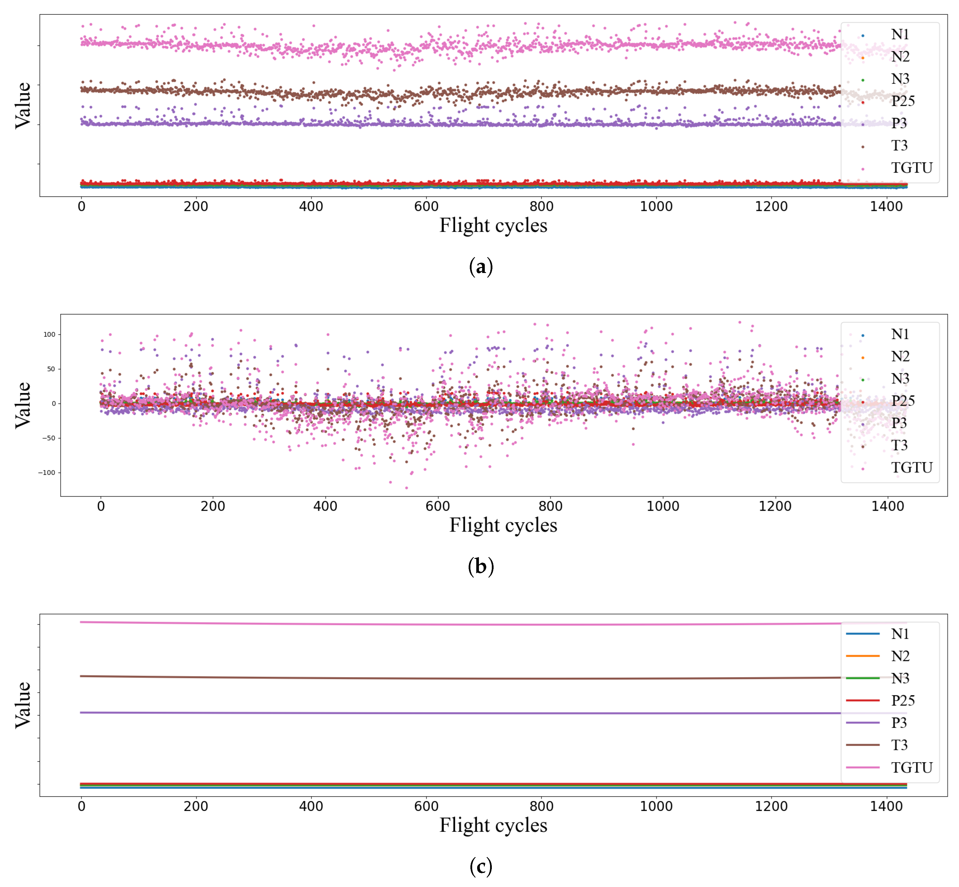
Figure 4 shows how detrending works on the given dataset. Examining the EHM data, some trends are apparent, such as long-term performance degradation and seasonality (Figure 4a). By removing these trends, the predictive model can focus on learning the underlying patterns in the residuals—specifically, the difference between the actual data and the trend (Figure 4b). Among various methods for detrending, polynomial fitting was adopted in this study. The polynomial function was fitted to the data, and its function values were subtracted from the original data during the preprocessing stage (Figure 4c).
Detrending is applied to both the train and test datasets before scaling. These detrended datasets are then used for model training, validation, and testing. Subsequently, the fitted trend is added to the prediction results to analyze model performance.

2.5. Multi-Engine-Based Large Generalized Model

The proposed models use smaller, segment-based training datasets, and each engine has its own individually trained models; however, there was interest in developing a multi-engine-based large generalized model for each turbofan engine family fleet. A generalized model, once trained, can be deployed to any engine without needing to develop a new model. To become a generalized model, the model should be trained on a larger training dataset that includes data from multiple engines. However, as the model becomes heavier, it requires greater computational resources and processing time.
To achieve a compromise between model accuracy and processing demands, the model used more but not all of the data, incorporating only the first segment of each engine as a training dataset. For each turbofan family engine, all of the first segments were combined and fed into the model for training (Figure 5). The trained models were tested on the remaining segments of each family engine, the same as Approach I. It is worth noting that if the train–test method was applied, the amount of training data would be approximately two times larger.

3. Machine Learning Algorithms

3.1. Long Short-Term Memory

As discussed in the introduction, it was found that long short-term memory (LSTM) has been one of the most widely used neural networks in machine learning (ML) approaches.
LSTM is a type of recurrent neural network (RNN). While RNNs have a chain-like structure suited for sequence data, they struggle with long-term dependencies in practice, despite their theoretical capability [37]. To address this, Hochreiter and Schmidhuber introduced LSTM [9], which improves learning by enhancing error backflow, solving the long-term dependency problem that hindered RNNs.
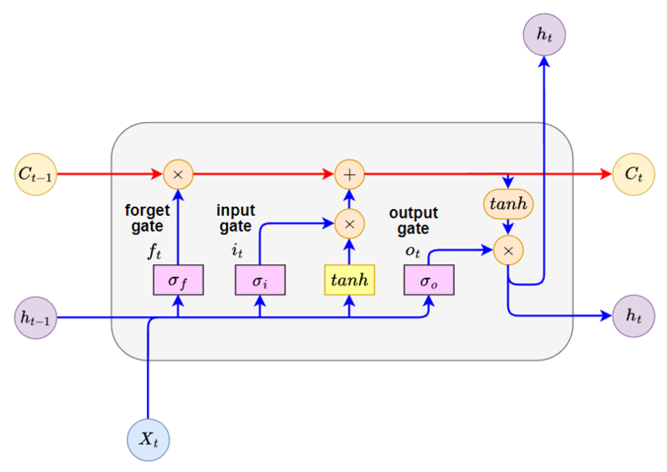
In general, standard RNNs contain a simple tan h layer within their modules, which are connected sequentially in a chain-like structure. In contrast, LSTM consists of four neural network layers interacting in a specialized way (Figure 6). The cell state running from C t 1 to C t is the key to LSTM (Equation (1e)). There are three gates regulating this cell state, which are composed of a sigmoid neural net ( σ ) and a point-wise multiplication operation. The sigmoid layer outputs numbers between zero and one, controlling how much of each component should be let through. A value of one lets everything through, and zero lets nothing through.
The three gates are called the forget ( σ f ), input ( σ i ), and output gates ( σ o ) (Equation (1a)–(1c)). The forget gate decides what information will be thrown away from the cell state. The input gate decides what new information will be stored in the cell state. At the end, the output gate decides on what will be output (Equation (1)). In this paper, the LSTM model employs a many-to-one architecture, processing a sequence of multiple data points and predicting turbine gas temperature (TGT) one at a time.
In Equation (1a), the input gate ( i t ) determines what new information from the current input ( X t ) and the previous hidden state ( h t 1 ) should be stored in the cell state ( C t ). The forget gate ( f t ) in Equation (1b) controls what information from the previous cell state ( C t 1 ) should be discarded or kept. The output gate ( o t ) (Equation (1c)) determines what part of the current cell state ( C t ) should be exposed as the hidden state ( h t ) for the current time step. The gate state ( g t ) in Equation (1d) computes a new candidate value that could be added to the cell state ( c t ). It processes the current input ( x t ) and the previous hidden state ( h t 1 ). Equation (1e) describes the cell state ( C t ), which is the core of LSTM, where the long-term memory (cell state) is updated. The hidden state ( h t ) represents the short-term memory or the output of the LSTM unit at the current time step. It is also the information passed to the next time step and is typically used for predictions or as input to subsequent layers.
i t = σ ( W i i X t + b i i + W h i h t 1 + b h i )
f t = σ ( W i f X t + b i f + W h f h t 1 + b h f )
o t = σ ( W i o X t + b i o + W h o h t 1 + b h o )
g t = tanh ( W i g X t + b i g + W h g h t 1 + b h g )
C t = f t C t 1 + i t g t
h t = o t tanh ( C t )

3.2. Linear and Nonlinear Algorithms

There are variations of LSTM [38,39,40,41] and hybrid models [39,41,42] that have demonstrated their prediction capability on the engine RUL prediction.
Instead of exploring variations of LSTM or any other neural network (NN) models, the authors decided to explore linear and nonlinear regression algorithms as a comparison to vanilla LSTM, the main model in this paper (Table 6). These are the most commonly used algorithms. The value of comparing linear and nonlinear regression algorithms to LSTM lies in understanding their relative strengths and weaknesses, which can inform the selection of the most appropriate algorithm for a given task. While linear algorithms offer simplicity and interpretability, nonlinear algorithms and NNs provide greater flexibility and representational power at the cost of increased complexity. Therefore, this comparison can provide meaningful insight in choosing the optimal algorithmic approach tailored to specific requirements for the engine prognostic model.
In this paper, the hyperparameters of LSTM, linear, and nonlinear regression algorithms, such as epochs, batch size, etc., were tuned using the grid search method [58]. The evaluation criterion for the grid search was the selection of the best model with the lowest loss on the validation dataset. The validation dataset was separated from the training segment prior to model training. Although it can be time-consuming due to its search strategy, it evaluates every possible combination of hyperparameters within the specified range. Based on a preliminary case study, and considering the scale of the dataset, a heuristic hyperparameter space was defined for exploration (Table 7).

4. Results

To evaluate the prediction results, the root mean squared error (RMSE) was calculated using the Equation (2):
RMSE = i = 1 N | y ^ i y i | 2 N
where y ^ is the predicted values, y is the actual values, and N is the number of non-missing data points. The RMSE values were calculated for each engine or test dataset, then their mean and median values were used to compare the performances of each machine learning (ML) algorithm, approach, and engine. The interquartile range (IQR) and outlier ratio were compared to measure the prediction performance and robustness of the models as well.
Due to the large dataset, a box plot was employed, incorporating a comparison between representative actual and predicted results.

4.1. Prediction Accuracies of Linear Algorithms, Nonlinear Algorithms, and LSTM

First, the prediction accuracy of each model—linear regression algorithms, nonlinear regression algorithms, and long short-term memory (LSTM)—is compared using the engine health monitoring (EHM) data of turbofan family engine A, as shown in Table 8. The table shows the mean, median, maximum, and minimum RMSE values, the IQR in [C], and the ratio of the outlier segment as a percentage. The minimum values among the linear and nonlinear regression algorithms are highlighted in bold text, respectively.
As long as the training approaches are consistent, there is no significant difference in the prediction accuracy between the algorithms. Among the nonlinear regression algorithms, support vector machine (svmr) consistently showed better accuracy across different training approaches than the others. No such pattern was observed among the linear regression algorithms.
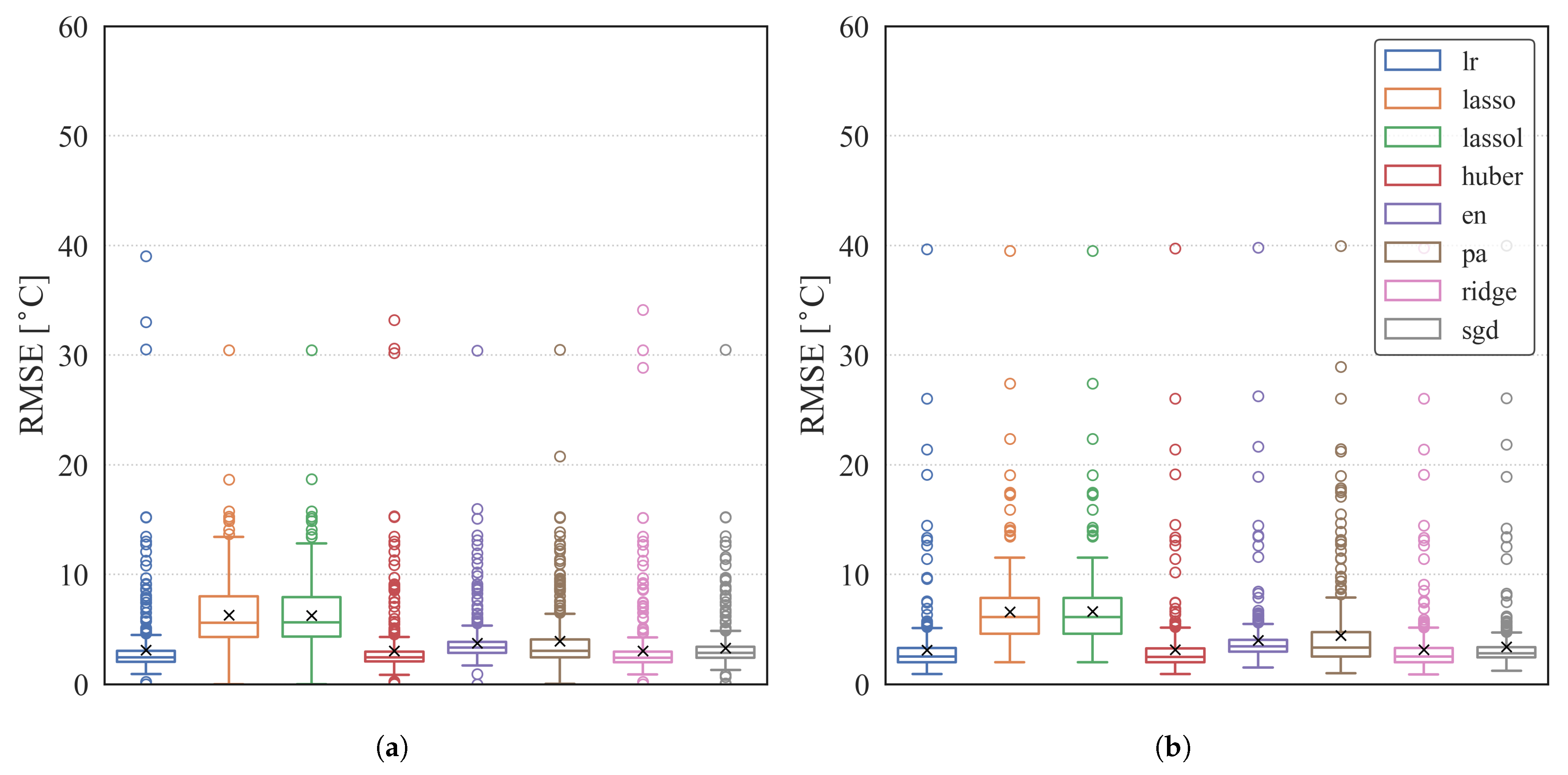
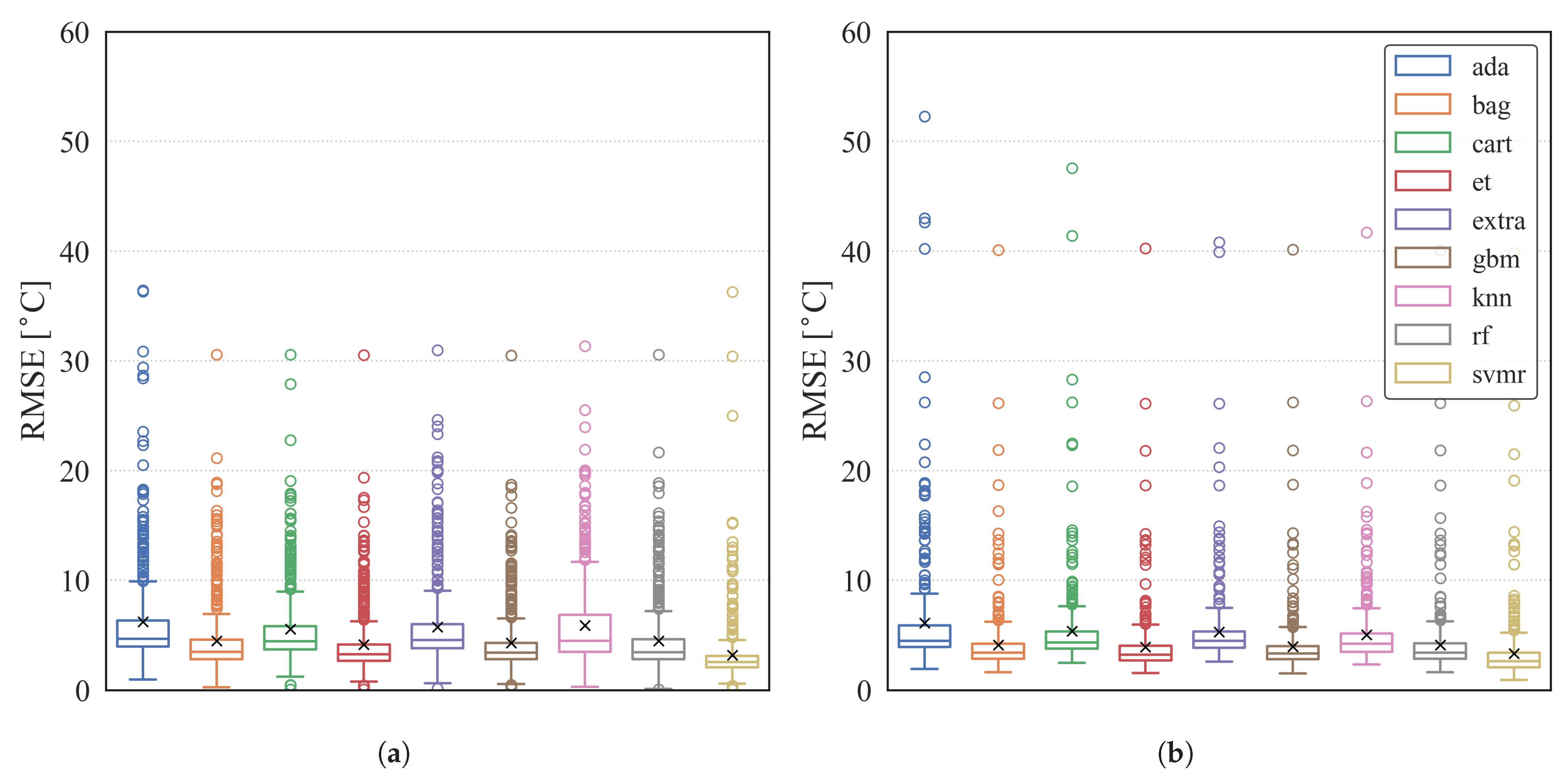
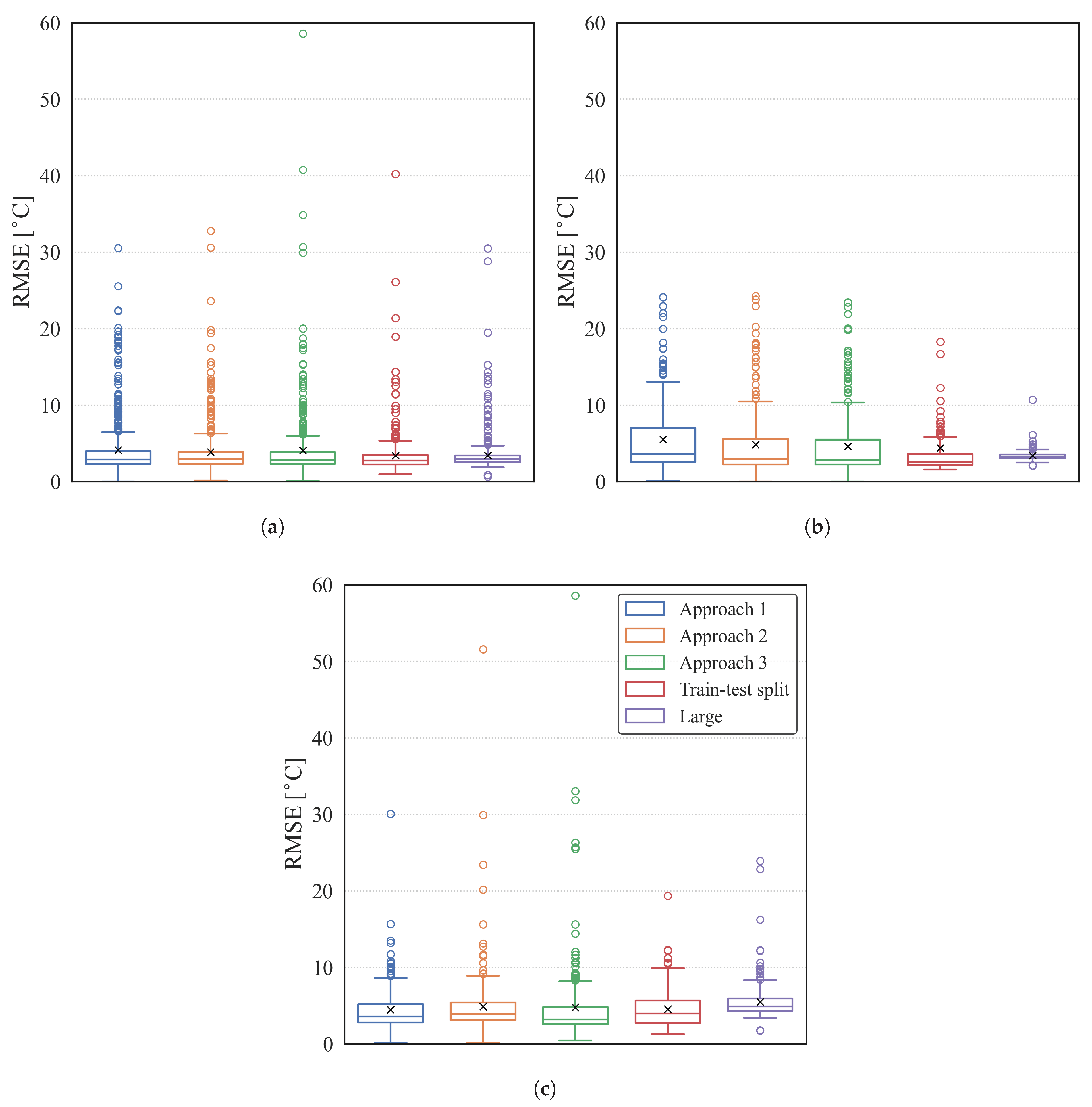
The same results are depicted in the box plots in Figure 7, Figure 8 and Figure 9a. The y-axis is the RMSE value in [C]; ‘x’ represents the mean; and the horizontal line inside of the box represents the median value. The size of the box plot represents the IQR, which is the distance between the 25th and 75th percentiles; the upper and lower whiskers show the minimum and maximum results excluding any outliers. The hollow dots represent the outliers. Here, the results of Approach I and the train–test split are presented, as Approaches II and III showed similar results to Approach I.
Table 8 and the box plot in Figure 7 show that the linear regression algorithms produced outliers in less than 10% of the total results, which is fewer than other nonlinear algorithms and LSTM. Nonlinear regression algorithms demonstrated similar results in terms of mean, median, maximum, and minimum RMSE compared to linear ones, but there were more outliers, ranging from 7% to 15%, as well as the LSTM models (Figure 8 and Figure 9a).
This observation implies that there is no significant difference between linear, nonlinear regression algorithms, and LSTM in providing turbine gas temperature (TGT) predictions. Furthermore, some algorithms, such as linear regression (lr), Huber regression (huber), ridge regression (ridge), and stochastic gradient descent regression (sgd) from linear regression algorithms, and support vector machine regression (svmr) from nonlinear regression algorithms, deliver prediction accuracy with a mean RMSE of less than 3.5 C and outliers of less than 10%. Additionally, these algorithms required less computational cost and time, taking less than a third of the training time compared to that of the LSTM models used.

4.2. Comparison of Prediction Accuracies of Training Approaches

The train–test split method is compared to the proposed segment-based training approaches. Table 9 summarizes the prediction results of all LSTM models on turbofan family engines A, B, and C.
Among the different approaches and models, the train–test split showed better prediction accuracy than the others, but the differences were less than 1 C in mean and median RMSE values. The large generalized models showed that there is less variability with smaller IQR values for all three turbofan family engines. It is worth noting that the three proposed segment-based approaches provided comparable prediction performance against the train–test split methods as well as the large models.
Figure 9 shows the box plots of the LSTM models for each turbofan family engine. The first notable observation is that all the data are right-skewed, indicated by mean values exceeding the median and mode values. Consequently, most of the results lie in the lower bound. This tendency was also observed in both the linear and nonlinear regression algorithms, as presented in Table 8. It is worth highlighting that the sizes of the boxes, i.e., IQR values, of the large models are the smallest. This suggests that the likelihood of better prediction is higher with more data, as it is likely to be more informative than a smaller dataset, such as a single segment between major overhauls.
Table 10 shows the normalized amount of data, i.e., engine cycles, used for model training and testing. The numbers are normalized to the amount of the train dataset of the train–test split method, respectively. It shows that the train-itest split method used up to about three times more data for model training than the segment-based approaches. It is worth noting that the size of training data for Approaches I and III on turbofan family engine C is smaller than that of the test data.
Additionally, comparing median RMSE values indicates that all of the models were able to predict TGT in 5 C of the mean RMSE value for the individual engines (Table 9).

4.3. Result of Multi-Engine-Based Large Generalized Model

The multi-engine-based large generalized models for all Turbofan family engines showed intriguing results. The most notable feature of these models is the very small IQR in their prediction results. In the case of turbofan family engine B, the model has significantly fewer extreme outliers, defined as those with mean RMSE values exceeding 20 C, compared to the other approaches. With only about 5.6% outliers from its test dataset, the model has the smallest portion of outliers among all within this engine family. Additionally, its mean RMSE is the lowest compared to other models in the same family. However, for the other two family engines A and C, the mean RMSE values are not the best, as the train–test split method and Approach I showed the lowest values, respectively. Nevertheless, considering the outlier ratio, the magnitude of the outliers, and the IQR values, the large generalized model for all three family engines provided more robust predictions.

4.4. Detail View of the Prediction Results

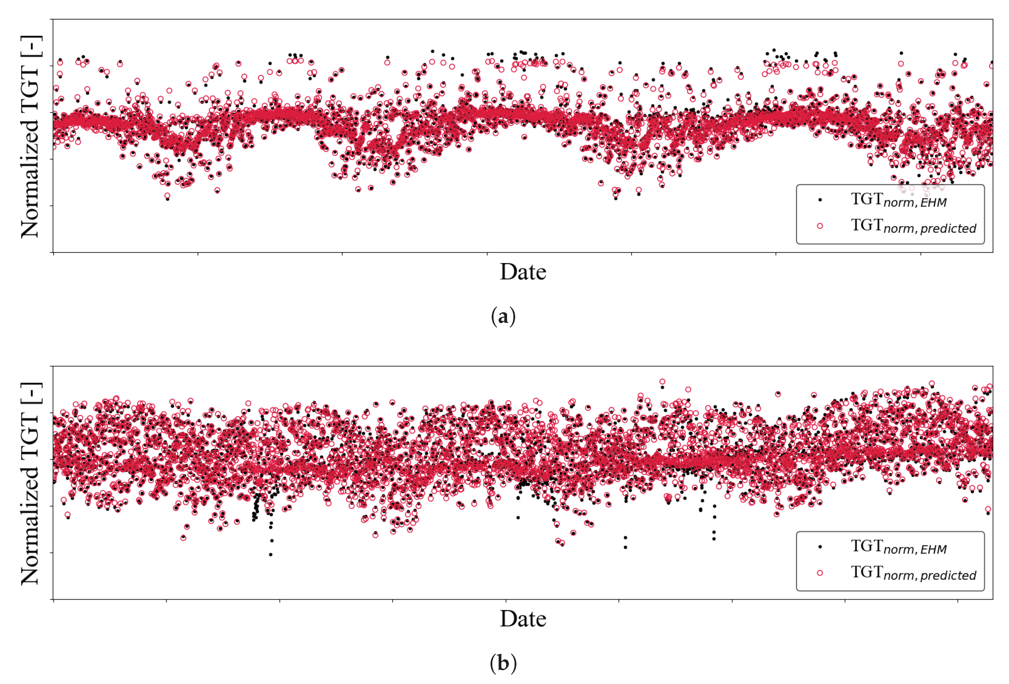
The prediction results of each model were discussed based on the box plots in the previous sections. The results showed that there are outliers depending on the family engines and the way the models were trained. It is worthwhile to compare the prediction results for the outliers with those within the interquartile range. The LSTM models’ prediction results are shown in Figure 10. The plots show the actual EHM TGT value (black solid dot) and the predicted TGT (red hollow circle) after normalization. Both values are normalized to the TGT value in the first cycle of the actual EHM data, as described in Equations (3) and (4). The x-axis is an engine cycle normalized to the first data point of the test dataset.
TGT norm , EHM = TGT EHM TGT EHM , 1 st   cycle
TGT norm , predicted = TGT predicted TGT EHM , 1 st   cycle
The prediction result near the mean value shows that each prediction matches each actual value and captures the changes in the TGT over its life cycle (Figure 10a). The model seems to become less accurate in predicting TGT where the points are far from the mean of the observed values.
Figure 10b shows one of the outlier results of the LSTM model prediction. Overall, the model was able to predict the target TGTEHM variations accurately. However, the presence of local deviations is worth noting. The total amount of local deviation is about 5% of the target TGT EHM. This characteristic prevails in every outlier from the various models tested, including linear and nonlinear regression algorithms and the LSTM model. The hyperparameter optimization was extended to address these outliers, but it did not improve the prediction accuracy.

4.5. Uncertainty Quantification

There has been research using neural networks to generate prediction intervals and quantify uncertainty. Initial research [59,60] established the foundational delta methodology for constructing asymptotically valid prediction intervals (PIs) in artificial neural networks (ANNs), exploring methods like weight decay. Subsequent work by Ho et al. (2001) [61] applied these PIs to nonlinear regression in manufacturing, while Khosravi et al. (2009) [62] optimized delta method networks using genetic algorithms to improve PI quality (width and coverage). Lu et al. (2009) [63] further investigated delta and bootstrap methods for PIs in nonlinear autoregressive with external input (NNARX) models for environmental predictions. Most recently, Wu et al. (2016) [64] developed an LSTM-based framework that uses k-means clustering and empirical probability density functions of error residuals to generate probabilistic forecasts and quantify uncertainty in wind power predictions.
Uncertainty quantification with the ‘Delta’ method was employed for multi-engine-based large models for all three turbofan family engines (Table 11). The following evaluation metrics were used: prediction interval coverage probability (PICP) [65,66,67,68], mean prediction interval width (MPIW), normalized mean prediction interval width (NMPIW), and coverage width criterion (CWC) [69]:
PICP = 1 N i = 1 N 1 · y i [ L ^ i , U ^ i ] ,
where ( 1 · ) is the indicator function, yielding 1 if y i is encompassed by the interval ([ L ^ i , U ^ i ]), and 0 otherwise. Typically, a coverage level close to the nominal confidence (e.g., 95%) is desired.
MPIW = 1 N i = 1 N U ^ i L ^ i
NMPIW = MPIW max i ( y i ) min i ( y i )
CWC = MPIW ,   if   PICP P * MPIW × 1 + exp η PICP P * ,   otherwise
Turbofan family engines A and C achieved 100% PICP, but their MPIWs were relatively wide (approx. 30 C), suggesting over-coverage or overly conservative intervals. Turbofan family engine C also had the highest MAE, indicating the least accurate point predictions. Turbofan family engine B offered the best balance: a strong 93% PICP with significantly narrower MPIWs value of 12.07 C and the lowest NMPIW, making its PIs more practical and precise. A notable observation was the zero StdPIW for all models, implying constant PI widths, which was unusual and suggested a specific, perhaps simplified, application of the Delta method. In essence, turbofan family engine B demonstrated the most effective UQ, providing accurate and practically useful prediction intervals, despite not having the absolute lowest point prediction error.
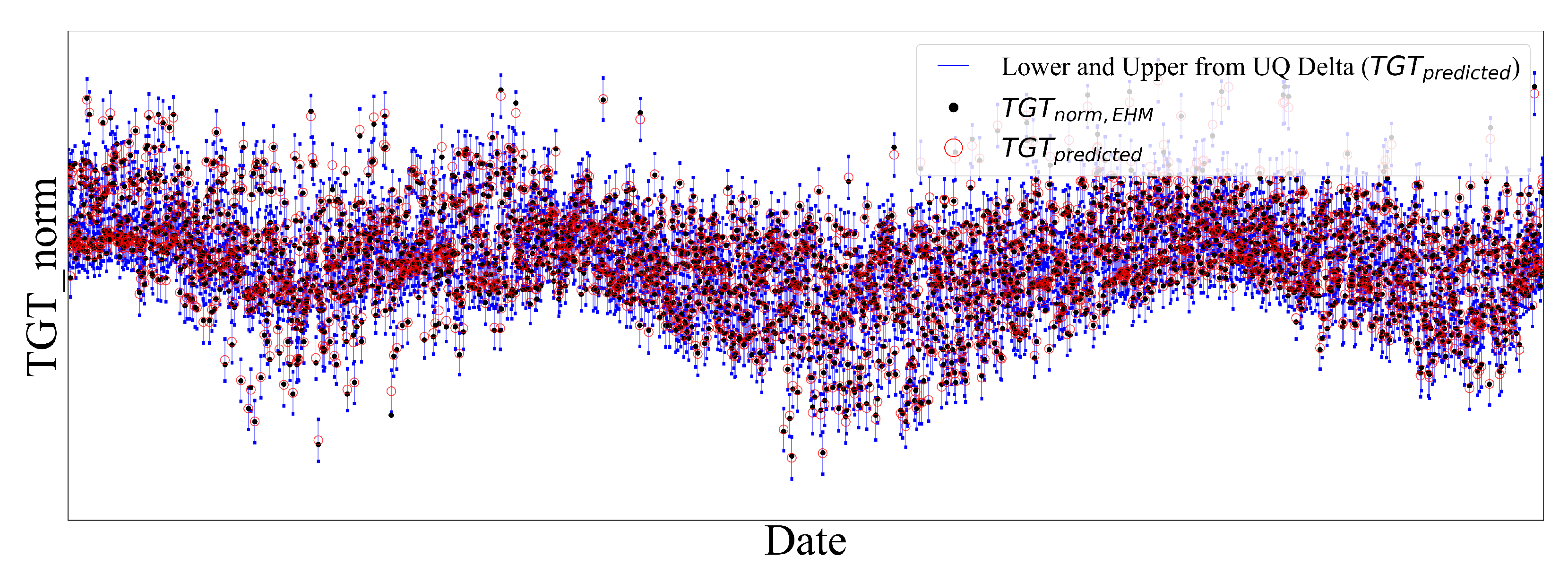
Figure 11 shows the sampled result of uncertainty quantification using the delta method for turbofan family engine A. The blue lines describe the range between the lower and upper bound from the Delta method. It shows that most of the target values (black dots) lay within the uncertainty range, as discussed above.

5. Conclusions

Building a predictive engine performance model has been of interest in the gas turbine and aerospace industry, yet it has been challenging to develop a robust and reliable model that characterizes individual engines that operate under various conditions and experience different flight cycles. Physics-based models are still widely used, but it is difficult to characterize the stochastic degradation behaviors of each component and system. This makes recent advancements in artificial intelligence (AI) and machine learning (ML) attractive to engineers, leading them to leverage these approaches to build and improve the forecasting capability of existing models.
This paper presents a selection of predictor variables, data segmentation to create training and test datasets, the application of detrending to help the models focus on substantial relationship between variables, and the evaluation of ML algorithms in the thorough prediction of turbine gas temperature (TGT). The engine health monitoring (EHM) data acquired from three different turbofan family engines were used. Observation of the characteristics of EHM data provided useful insights for selecting training approaches and the most effective set of predictor variables. New training approaches (Approaches I, II, and III) were proposed using data segmentation based on time between major overhauls. The prediction accuracies of the selected ML algorithms, including linear and nonlinear regression algorithms and long short-term memory (LSTM), were compared for individual engines. Further comparison was made by building a large generalized model for each turbofan family engine. The key findings are as follows:
-
The seven predictor variables of Set 4 showed a minimum percentage of outliers with comparable prediction accuracy among the other sets.
-
There were promising results from linear and nonlinear regression algorithms.
-
For individual engines, the proposed training approaches demonstrated their prediction capability with a mean root mean squared error (RMSE) ranging from 4 C to 6 C, utilizing up to 65% less data than the train (80%)–test (20%) split method.
-
The multi-engine-based large generalized model, by utilizing the data of each family engine, achieved similar prediction accuracy (a mean RMSE ranging from 3 C to 5 C) with smaller IQR (from 0.5 C to 1.6 C); however, the amount of data required was 45–300 times larger than the proposed approaches.
-
Uncertainty quantification showed a coverage width criterion (CWC) between 29 C and 40 C, varying with different engine families. The prediction interval coverage probability (PICP) was over 93% for all engines.
The amount of training datasets used for new segment-based training approaches was significantly less than that of the train (80%)–test (20%) split method and the large generalized model, respectively, for each turbofan family engine. Nevertheless, the prediction results of the proposed approaches follow and capture the pattern and behavior of the target TGT value. The results imply that a predictive model can be developed even only when a limited amount of data is available. Since “big and complete” datasets do not always exist or are not always available, this finding offers an opportunity to build a predictive engine health model in the early stages of engine development and service operation.
The proposed framework was developed and validated utilizing the in-service EHM datasets of three different turbofan family engines. Hence, the key findings on predictor variables, data segmentation, and machine learning algorithms are robust enough to suggest wider applications. Furthermore, the sensitivity of the amount of training data to the prediction accuracy provides useful insight when applying the framework, even for engines with relatively small datasets.

6. Future Research

This is one of the few attempts to build a predictive engine performance model applying machine learning (ML) to in-service engine health monitoring (EHM) data. The authors are enthusiastic about further developing the model. The following list proposes further research topics to enhance data processing, prediction accuracy, and explain the underlying principles behind the in-service data:
-
Incorporate ancillary data such as flight routes, weather, and airborne particulates.
-
Implement missing value imputation.
-
Apply advanced algorithms.
-
Examine uncertainty quantification (UQ) methods.

Author Contributions

Conceptualization, J.-S.J. and C.S.; Investigation, J.-S.J.; Methodology, J.-S.J.; Project administration, A.R. and R.J.C.; Resources, A.R.; Supervision, C.S., A.R. and R.J.C.; Visualization, J.-S.J.; Writing—original draft, J.-S.J.; Writing—review and editing, C.S. All authors have read and agreed to the published version of the manuscript.

Funding

This research was sponsored by Rolls-Royce and Virginia Tech.

Data Availability Statement

The data that support the findings of this study were made available from Rolls-Royce plc, but restrictions apply to the availability of these data, which were used under license for the current study and are not publicly available. Point of contact for data requests: changminson@vt.edu.

Acknowledgments

The authors appreciate the technical and financial support from Rolls-Royce and Virginia Tech. The authors extend special thanks to Jostein Barry-Straume and Adrian Sandu for technical discussion about ML algorithms and contribution to the uncertainty quantification analysis.

Conflicts of Interest

Authors Andrew Rimell, and Rory J. Clarkson were employed by Rolls-Royce plc. The remaining authors declare that the research was conducted in the absence of any commercial or financial relationships that could be construed as a potential conflict of interest. The authors declare that this study received funding from Rolls-Royce plc. The funder approved the publication of this article.

Abbreviations

The following abbreviations are used in this manuscript:
adaadaboost regression
bagbagging regression
cartdecision tree regression
C-MAPSSCommercial Modular Aero-Propulsion System Simulation
CWCcoverage width criterion
EHMengine health monitoring
enelastic net regression
extraextra trees regression
gbmgradient boosting machine
HPChigh-pressure compressor
huberHuber regression
IPCintermediate pressure compressor
IQRinterquantile range
knnk-nearest neighbors regression
lassolasso linear regression
lassollasso least angle regression (lars)
lrlinear regression
LSTMlong short-term-memory
Max.maximum value
Min.minimum value
MPIWmean prediction interval width
NMPIWnormalized mean prediction interval width
outlierratio of outlier
papassive aggressive regression
PICPprediction interval coverage probability
rfrandom forest regression
ridgeridge regression
RMSEroot mean squared error
RULremaining useful life
sgdstochastic gradient descent regression
StdAEstandard deviation of absolute error
StdPIWstandard deviation of prediction interval width
svmrsupport vector machine regression
TGTturbine gas temperature
y ^ predicted value
y i actual (target) value

Appendix A. Studies Utilizing NASA C-MAPSS Dataset

To provide comprehensive detail for the consolidated “NASA C-MAPSS Studies” entry in Table 1, the following references are those identified in the literature survey that utilized the NASA C-MAPSS dataset for their prognostic analysis. The number of variables used by each study can vary, typically due to feature selection or different sub-datasets of C-MAPSS.
Table A1. References using NASA C-MAPSS dataset and their variable counts.
ReferenceNo. Var.ReferenceNo. Var.ReferenceNo. Var.ReferenceNo. Var.
[3]14[70]30/18[71]26[72]14
[73]21[74]14[75]26[76]14
[77]26[78]26[38]14[79]14
[6]7[80]26[81]26[82]14–17
[83]24[84]11[85]26[86]46
[39]26[87]14[88]24[89]14
[90]21[91]14[92]24[93]14
[40]26[94]21[42]21[95]7
[41]14[96]26[97]24[98]14
[99]14[100]26[101]26[102]10–20
[103]24[104]24

References

  1. Schwabacher, M. A Survey of Data-Driven Prognostics. In Proceedings of the Infotech@Aerospace, Arlington, VI, USA, 26–29 September 2005; p. 7002. [Google Scholar] [CrossRef]
  2. Schwabacher, M.; Goebel, K. A Survey of Artificial Intelligence for Prognostics. In AAAI Fall Symposium: Artificial Intelligence for Prognostics; Association for the Advancement of Artificial Intelligence: Washington, DC, USA, 2007; pp. 108–115. [Google Scholar]
  3. Saxena, A.; Goebel, K.; Simon, D.; Eklund, N. Damage propagation modeling for aircraft engine run-to-failure simulation. In Proceedings of the 2008 International Conference on Prognostics and Health Management, Denver, CO, USA, 6–9 October 2008; IEEE: New York, NY, USA, 2008; pp. 1–9. [Google Scholar]
  4. Li, Y.G. Gas turbine performance and health status estimation using adaptive gas path analysis. J. Eng. Gas Turbines Power 2010, 132, 041701. [Google Scholar] [CrossRef]
  5. Pinelli, M.; Spina, P.R.; Venturini, M. Gas turbine health state determination: Methodology approach and field application. Int. J. Rotating Mach. 2012, 2012, 142173. [Google Scholar] [CrossRef]
  6. Alozie, O.; Li, Y.G.; Wu, X.; Shong, X.; Ren, W. An adaptive model-based framework for prognostics of gas path faults in aircraft gas turbine engines. Int. J. Progn. Health Manag. 2019, 10, 013. [Google Scholar] [CrossRef]
  7. Fang, Y.l.; Liu, D.f.; Liu, Y.b.; Yu, L.w. Comprehensive assessment of gas turbine health condition based on combination weighting of subjective and objective. Int. J. Gas Turbine Propuls. Power Syst. 2020, 11, 56–62. [Google Scholar] [CrossRef]
  8. LeCun, Y.; Bengio, Y.; Hinton, G. Deep Learning. Nature 2015, 521, 436–444. [Google Scholar] [CrossRef]
  9. Hochreiter, S.; Schmidhuber, J. Long short-term memory. Neural Comput. 1997, 9, 1735–1780. [Google Scholar] [CrossRef]
  10. Frederick, D.K.; DeCastro, J.A.; Litt, J.S. User’s Guide for the Commercial Modular Aero-Propulsion System Simulation (C-MAPSS); Technical Report; Glenn Research Center: Cleveland, OH, USA, 2007. [Google Scholar]
  11. CMAPSS Jet Engine Simulated Data, NASA Open Data Portal. 2016. Available online: https://data.nasa.gov/dataset/cmapss-jet-engine-simulated-data (accessed on 23 January 2025).
  12. Marinai, L. Gas-Path Diagnostics and Prognostics for Aero-Engines Using Fuzzy Logic and Time Series Analysis. Ph.D. Thesis, School of Engineering, Canfield University, Canfield, OH, USA, 2004. [Google Scholar]
  13. Spieler, S.; Staudacher, S.; Fiola, R.; Sahm, P.; Weißschuh, M. Probabilistic Engine Performance Scatter and Deterioration Modeling. In Proceedings of the ASME Turbo Expo 2007: Power for Land, Sea, and Air, Montreal, QC, Canada, 14–17 May 2007; American Society of Mechanical Engineers Digital Collection: New York, NY, USA, 2009; pp. 1073–1082. [Google Scholar] [CrossRef]
  14. Martínez, A.; Sánchez, L.; Couso, I. Engine Health Monitoring for Engine Fleets Using Fuzzy Radviz. In Proceedings of the 2013 IEEE International Conference on Fuzzy Systems (FUZZ-IEEE), Hyderabad, India, 7–10 July 2013; pp. 1–8. [Google Scholar] [CrossRef]
  15. Martinez, A.; Sánchez, L.; Couso, I. Aeroengine Prognosis through Genetic Distal Learning Applied to Uncertain Engine Health Monitoring Data. In Proceedings of the 2014 IEEE International Conference on Fuzzy Systems (FUZZ-IEEE), Beijing, China, 6–11 July 2014; pp. 1945–1952. [Google Scholar] [CrossRef]
  16. Gräter, F.; Staudacher, S.; Weißschuh, M. Operator-Specific Engine Trending Using a Feature-Based Model. In Proceedings of the ASME Turbo Expo 2010: Power for Land, Sea, and Air, Glasgow, UK, 14–18 June 2010; American Society of Mechanical Engineers Digital Collection: New York, NY, USA, 2010; pp. 79–88. [Google Scholar] [CrossRef]
  17. Skaf, Z.; Zaidan, M.A.; Harrison, R.F.; Mills, A.R. Accommodating Repair Actions into Gas Turbine Prognostics. In Proceedings of the Annual Conference of the PHM Society, New Orleans, LA, USA, 14–17 October 2013; Volume 5. [Google Scholar] [CrossRef]
  18. Laslett, O.W.; Mills, A.R.; Zaidan, M.A.; Harrison, R.F. Fusing an Ensemble of Diverse Prognostic Life Predictions. In Proceedings of the 2014 IEEE Aerospace Conference, Big Sky, MT, USA, 1–8 March 2014; pp. 1–10. [Google Scholar] [CrossRef]
  19. Olausson, P.; Häggståhl, D.; Arriagada, J.; Dahlquist, E.; Assadi, M. Hybrid model of an evaporative gas turbine power plant utilizing physical models and artificial neural networks. In Proceedings of the Turbo Expo: Power for Land, Sea, and Air, Atlanta, GA, USA, 16–19 June 2003; Volume 36843, pp. 299–306. [Google Scholar]
  20. Fast, M.; Assadi, M.; De, S. Condition based maintenance of gas turbines using simulation data and artificial neural network: A demonstration of feasibility. In Proceedings of the Turbo Expo: Power for Land, Sea, and Air, Berlin, Germany, 9–13 June 2008; Volume 43123, pp. 153–161. [Google Scholar]
  21. Vatani, A.; Khorasani, K.; Meskin, N. Health monitoring and degradation prognostics in gas turbine engines using dynamic neural networks. In Proceedings of the Turbo Expo: Power for Land, Sea, and Air, Montreal, QC, Canada, 15–19 June 2015; American Society of Mechanical Engineers: New York, NY, USA, 2015; Volume 56758, p. V006T05A030. [Google Scholar]
  22. Zaidan, M.A.; Harrison, R.F.; Mills, A.R.; Fleming, P.J. Bayesian hierarchical models for aerospace gas turbine engine prognostics. Expert Syst. Appl. 2015, 42, 539–553. [Google Scholar] [CrossRef]
  23. Zaidan, M.A.; Relan, R.; Mills, A.R.; Harrison, R.F. Prognostics of gas turbine engine: An integrated approach. Expert Syst. Appl. 2015, 42, 8472–8483. [Google Scholar] [CrossRef]
  24. Pillai, P.; Kaushik, A.; Bhavikatti, S.; Roy, A.; Kumar, V. A hybrid approach for fusing physics and data for failure prediction. Int. J. Progn. Health Manag. 2016, 7, 4. [Google Scholar] [CrossRef]
  25. Yang, X.; Pang, S.; Shen, W.; Lin, X.; Jiang, K.; Wang, Y. Aero engine fault diagnosis using an optimized extreme learning machine. Int. J. Aerosp. Eng. 2016, 2016, 7892875. [Google Scholar] [CrossRef]
  26. Khan, F.; Eker, O.; Khan, A.; Orfali, W. Adaptive Degradation Prognostic Reasoning by Particle Filter with a Neural Network Degradation Model for Turbofan Jet Engine. Data 2018, 3, 49. [Google Scholar] [CrossRef]
  27. Yildirim, M.T.; Kurt, B. Aircraft gas turbine engine health monitoring system by real flight data. Int. J. Aerosp. Eng. 2018, 2018, 9570873. [Google Scholar] [CrossRef]
  28. Kim, S.; Kim, K.; Son, C. Transient system simulation for an aircraft engine using a data-driven model. Energy 2020, 196, 117046. [Google Scholar] [CrossRef]
  29. Fentaye, A.; Zaccaria, V.; Rahman, M.; Stenfelt, M.; Kyprianidis, K. Hybrid model-based and data-driven diagnostic algorithm for gas turbine engines. In Proceedings of the Turbo Expo: Power for Land, Sea, and Air, Online, 21–25 September 2020; American Society of Mechanical Engineers: New York, NY, USA, 2020; Volume 84140, p. V005T05A008. [Google Scholar]
  30. Lin, L.; Liu, J.; Guo, H.; Lv, Y.; Tong, C. Sample adaptive aero-engine gas-path performance prognostic model modeling method. Knowl.-Based Syst. 2021, 224, 107072. [Google Scholar] [CrossRef]
  31. Ullah, S.; Li, S.; Khan, K.; Khan, S.; Khan, I.; Eldin, S.M. An Investigation of Exhaust Gas Temperature of Aircraft Engine Using LSTM. IEEE Access 2023, 11, 5168–5177. [Google Scholar] [CrossRef]
  32. Xiao, W.; Chen, Y.; Zhang, H.; Shen, D. Remaining Useful Life Prediction Method for High Temperature Blades of Gas Turbines Based on 3D Reconstruction and Machine Learning Techniques. Appl. Sci. 2023, 13, 11079. [Google Scholar] [CrossRef]
  33. Lee, D.; Kwon, H.J.; Choi, K. Risk-Based Maintenance Optimization of Aircraft Gas Turbine Engine Component. Proc. Inst. Mech. Eng. Part O J. Risk Reliab. 2024, 238, 429–445. [Google Scholar] [CrossRef]
  34. Wold, S.; Esbensen, K.; Geladi, P. Principal Component Analysis. Chemom. Intell. Lab. Syst. 1987, 2, 37–52. [Google Scholar] [CrossRef]
  35. Abdi, H.; Williams, L.J. Principal Component Analysis. Wires Comput. Stat. 2010, 2, 433–459. [Google Scholar] [CrossRef]
  36. Pearson, K. Note on regression and inheritance in the case of two parents. Proc. R. Soc. Lond. 1895, 58, 240–242. [Google Scholar] [CrossRef]
  37. Bengio, Y.; Simard, P.; Frasconi, P. Learning long-term dependencies with gradient descent is difficult. IEEE Trans. Neural Netw. 1994, 5, 157–166. [Google Scholar] [CrossRef] [PubMed]
  38. Wang, J.; Wen, G.; Yang, S.; Liu, Y. Remaining Useful Life Estimation in Prognostics Using Deep Bidirectional LSTM Neural Network. In Proceedings of the 2018 Prognostics and System Health Management Conference (PHM-Chongqing), Chongqing, China, 26–28 October 2018; pp. 1037–1042. [Google Scholar] [CrossRef]
  39. Remadna, I.; Terrissa, S.L.; Zemouri, R.; Ayad, S.; Zerhouni, N. Leveraging the Power of the Combination of CNN and Bi-Directional LSTM Networks for Aircraft Engine RUL Estimation. In Proceedings of the 2020 Prognostics and Health Management Conference (PHM-Besançon), Besancon, France, 4–7 May 2020; pp. 116–121. [Google Scholar] [CrossRef]
  40. Shah, S.R.B.; Chadha, G.S.; Schwung, A.; Ding, S.X. A Sequence-to-Sequence Approach for Remaining Useful Lifetime Estimation Using Attention-augmented Bidirectional LSTM. Intell. Syst. Appl. 2021, 10–11, 200049. [Google Scholar] [CrossRef]
  41. Song, Y.; Gao, S.; Li, Y.; Jia, L.; Li, Q.; Pang, F. Distributed Attention-Based Temporal Convolutional Network for Remaining Useful Life Prediction. IEEE Internet Things J. 2021, 8, 9594–9602. [Google Scholar] [CrossRef]
  42. Song, J.W.; Park, Y.I.; Hong, J.J.; Kim, S.G.; Kang, S.J. Attention-Based Bidirectional LSTM-CNN Model for Remaining Useful Life Estimation. In Proceedings of the 2021 IEEE International Symposium on Circuits and Systems (ISCAS), Daegu, Republic of Korea, 22–28 May 2021; pp. 1–5. [Google Scholar] [CrossRef]
  43. Cover, T.; Hart, P. Nearest neighbor pattern classification. IEEE Trans. Inf. Theory 1967, 13, 21–27. [Google Scholar] [CrossRef]
  44. Tibshirani, R. Regression shrinkage and selection via the lasso. J. R. Stat. Soc. Ser. B (Methodol.) 1996, 58, 267–288. [Google Scholar] [CrossRef]
  45. Loh, W.Y. Classification and regression trees. Wiley Interdiscip. Rev. Data Min. Knowl. Discov. 2011, 1, 14–23. [Google Scholar] [CrossRef]
  46. Hoerl, A.E.; Kennard, R.W. Ridge regression: Biased estimation for nonorthogonal problems. Technometrics 1970, 12, 55–67. [Google Scholar] [CrossRef]
  47. Geurts, P.; Ernst, D.; Wehenkel, L. Extremely randomized trees. Mach. Learn. 2006, 63, 3–42. [Google Scholar] [CrossRef]
  48. Zou, H.; Hastie, T. Regularization and variable selection via the elastic net. J. R. Stat. Soc. Ser. B (Stat. Methodol.) 2005, 67, 301–320. [Google Scholar] [CrossRef]
  49. Drucker, H.; Burges, C.J.; Kaufman, L.; Smola, A.; Vapnik, V. Support vector regression machines. In Proceedings of the 10th International Conference on Neural Information Processing Systems, Denver, CO, USA, 3–5 December 1996; Volume 9. [Google Scholar]
  50. Huber, P.J. Robust regression: Asymptotics, conjectures and Monte Carlo. Ann. Stat. 1973, 1, 799–821. [Google Scholar] [CrossRef]
  51. Freund, Y.; Schapire, R.; Abe, N. A short introduction to boosting. J.-Jpn. Soc. Artif. Intell. 1999, 14, 1612. [Google Scholar]
  52. Efron, B.; Hastie, T.; Johnstone, I.; Tibshirani, R. Least angle regression. Ann. Stat. 2004, 32, 407–499. [Google Scholar] [CrossRef]
  53. Breiman, L. Bagging predictors. Mach. Learn. 1996, 24, 123–140. [Google Scholar] [CrossRef]
  54. Crammer, K.; Dekel, O.; Keshet, J.; Shalev-Shwartz, S.; Singer, Y. Online passive aggressive algorithms. J. Mach. Learn. Res. 2006, 7, 551–585. [Google Scholar]
  55. Breiman, L. Random forests. Mach. Learn. 2001, 45, 5–32. [Google Scholar] [CrossRef]
  56. Kiefer, J.; Wolfowitz, J. Stochastic estimation of the maximum of a regression function. Ann. Math. Stat. 1952, 23, 462–466. [Google Scholar] [CrossRef]
  57. Friedman, J.H. Greedy function approximation: A gradient boosting machine. Ann. Stat. 2001, 29, 1189–1232. [Google Scholar] [CrossRef]
  58. Liashchynskyi, P.; Liashchynskyi, P. Grid Search, Random Search, Genetic Algorithm: A Big Comparison for NAS. arXiv 2019, arXiv:1912.06059. [Google Scholar] [CrossRef]
  59. Hwang, J.G.; Ding, A.A. Prediction intervals for artificial neural networks. J. Am. Stat. Assoc. 1997, 92, 748–757. [Google Scholar] [CrossRef]
  60. De Vleaux, R.D.; Schumi, J.; Schweinsberg, J.; Ungar, L.H. Prediction intervals for neural networks via nonlinear regression. Technometrics 1998, 40, 273–282. [Google Scholar] [CrossRef]
  61. Ho, S.L.; Xie, M.; Tang, L.; Xu, K.; Goh, T. Neural network modeling with confidence bounds: A case study on the solder paste deposition process. IEEE Trans. Electron. Packag. Manuf. 2001, 24, 323–332. [Google Scholar] [CrossRef]
  62. Khosravi, A.; Nahavandi, S.; Creighton, D. Improving prediction interval quality: A genetic algorithm-based method applied to neural networks. In Proceedings of the Neural Information Processing: 16th International Conference, ICONIP 2009, Bangkok, Thailand, 1–5 December 2009; Proceedings, Part II 16. Springer: Berlin/Heidelberg, Germany, 2009; pp. 141–149. [Google Scholar]
  63. Lu, T.; Viljanen, M. Prediction of indoor temperature and relative humidity using neural network models: Model comparison. Neural Comput. Appl. 2009, 18, 345–357. [Google Scholar] [CrossRef]
  64. Wu, W.; Chen, K.; Qiao, Y.; Lu, Z. Probabilistic short-term wind power forecasting based on deep neural networks. In Proceedings of the 2016 International Conference on Probabilistic Methods Applied to Power Systems (PMAPS), Beijing, China, 16–20 October 2016; IEEE: New York, NY, USA, 2016; pp. 1–8. [Google Scholar]
  65. Van Hinsbergen, C.I.; Van Lint, J.; Van Zuylen, H. Bayesian committee of neural networks to predict travel times with confidence intervals. Transp. Res. Part C Emerg. Technol. 2009, 17, 498–509. [Google Scholar] [CrossRef]
  66. Zhao, J.H.; Dong, Z.Y.; Xu, Z.; Wong, K.P. A statistical approach for interval forecasting of the electricity price. IEEE Trans. Power Syst. 2008, 23, 267–276. [Google Scholar] [CrossRef]
  67. Pierce, S.G.; Worden, K.; Bezazi, A. Uncertainty analysis of a neural network used for fatigue lifetime prediction. Mech. Syst. Signal Process. 2008, 22, 1395–1411. [Google Scholar] [CrossRef]
  68. Zhang, C.; Wei, H.; Xie, L.; Shen, Y.; Zhang, K. Direct interval forecasting of wind speed using radial basis function neural networks in a multi-objective optimization framework. Neurocomputing 2016, 205, 53–63. [Google Scholar] [CrossRef]
  69. Khosravi, A.; Nahavandi, S.; Creighton, D.; Atiya, A.F. Comprehensive Review of Neural Network-Based Prediction Intervals and New Advances. IEEE Trans. Neural Netw. 2011, 22, 1341–1356. [Google Scholar] [CrossRef]
  70. Chao, M.A.; Kulkarni, C.; Goebel, K.; Fink, O. Fusing physics-based and deep learning models for prognostics. Reliab. Eng. Syst. Saf. 2022, 217, 107961. [Google Scholar] [CrossRef]
  71. Sateesh Babu, G.; Zhao, P.; Li, X.L. Deep convolutional neural network based regression approach for estimation of remaining useful life. In Proceedings of the International Conference on Database Systems for Advanced Applications, Dallas, TX, USA, 16–19 April 2016; Springer: Berlin/Heidelberg, Germany, 2016; pp. 214–228. [Google Scholar]
  72. Thakkar, U.; Chaoui, H. Remaining Useful Life Prediction of an Aircraft Turbofan Engine Using Deep Layer Recurrent Neural Networks. Actuators 2022, 11, 67. [Google Scholar] [CrossRef]
  73. Yuan, M.; Wu, Y.; Lin, L. Fault diagnosis and remaining useful life estimation of aero engine using LSTM neural network. In Proceedings of the 2016 IEEE International Conference on Aircraft Utility Systems (AUS), Beijing, China, 10–12 October 2016; IEEE: New York, NY, USA, 2016; pp. 135–140. [Google Scholar]
  74. Wang, T.; Guo, D.; Sun, X.M. Remaining Useful Life Predictions for Turbofan Engine Degradation Based on Concurrent Semi-Supervised Model. Neural Comput. Appl. 2022, 34, 5151–5160. [Google Scholar] [CrossRef]
  75. Zheng, S.; Ristovski, K.; Farahat, A.; Gupta, C. Long short-term memory network for remaining useful life estimation. In Proceedings of the 2017 IEEE International Conference on Prognostics and Health Management (ICPHM), Dallas, TX, USA, 19–21 June 2017; IEEE: New York, NY, USA, 2017; pp. 88–95. [Google Scholar]
  76. Xu, T.; Han, G.; Gou, L.; Martínez-García, M.; Shao, D.; Luo, B.; Yin, Z. SGBRT: An Edge-Intelligence Based Remaining Useful Life Prediction Model for Aero-Engine Monitoring System. IEEE Trans. Netw. Sci. Eng. 2022, 9, 3112–3122. [Google Scholar] [CrossRef]
  77. Hsu, C.S.; Jiang, J.R. Remaining useful life estimation using long short-term memory deep learning. In Proceedings of the 2018 IEEE International Conference on Applied System Invention (ICASI), Chiba, Japan, 13–17 April 2018; IEEE: New York, NY, USA, 2018; pp. 58–61. [Google Scholar]
  78. Alomari, Y.; Andó, M.; Baptista, M.L. Advancing Aircraft Engine RUL Predictions: An Interpretable Integrated Approach of Feature Engineering and Aggregated Feature Importance. Sci. Rep. 2023, 13, 13466. [Google Scholar] [CrossRef] [PubMed]
  79. Ensarioğlu, K.; İnkaya, T.; Emel, E. Remaining Useful Life Estimation of Turbofan Engines with Deep Learning Using Change-Point Detection Based Labeling and Feature Engineering. Appl. Sci. 2023, 13, 11893. [Google Scholar] [CrossRef]
  80. Keshun, Y.; Guangqi, Q.; Yingkui, G. A 3D Attention-enhanced Hybrid Neural Network for Turbofan Engine Remaining Life Prediction Using CNN and BiLSTM Models. IEEE Sens. J. 2023, 24, 21893–21905. [Google Scholar] [CrossRef]
  81. Miao, H.; Li, B.; Sun, C.; Liu, J. Joint Learning of Degradation Assessment and RUL Prediction for Aeroengines via Dual-Task Deep LSTM Networks. IEEE Trans. Ind. Inform. 2019, 15, 5023–5032. [Google Scholar] [CrossRef]
  82. Hu, Q.; Zhao, Y.; Ren, L. Novel Transformer-Based Fusion Models for Aero-Engine Remaining Useful Life Estimation. IEEE Access 2023, 11, 52668–52685. [Google Scholar] [CrossRef]
  83. Pasa, G.D.; Medeiros, I.; Yoneyama, T. Operating condition-invariant neural network-based prognostics methods applied on turbofan aircraft engines. In Proceedings of the Annual Conference of the PHM Society, Scottsdale, AZ, USA, 23–26 September 2019; Volume 11, pp. 1–10. [Google Scholar]
  84. Liu, Z.; Zhang, X.; Pan, J.; Zhang, X.; Hong, W.; Wang, Z.; Wang, Z.; Miao, Y. Similar or Unknown Fault Mode Detection of Aircraft Fuel Pump Using Transfer Learning With Subdomain Adaption. IEEE Trans. Instrum. Meas. 2023, 72, 3526411. [Google Scholar] [CrossRef]
  85. Wu, Z.; Yu, S.; Zhu, X.; Ji, Y.; Pecht, M. A Weighted Deep Domain Adaptation Method for Industrial Fault Prognostics According to Prior Distribution of Complex Working Conditions. IEEE Access 2019, 7, 139802–139814. [Google Scholar] [CrossRef]
  86. Maulana, F.; Starr, A.; Ompusunggu, A.P. Explainable Data-Driven Method Combined with Bayesian Filtering for Remaining Useful Lifetime Prediction of Aircraft Engines Using NASA CMAPSS Datasets. Machines 2023, 11, 163. [Google Scholar] [CrossRef]
  87. Sharanya, S.; Venkataraman, R.; Murali, G. Predicting Remaining Useful Life of Turbofan Engines Using Degradation Signal Based Echo State Network. Int. J. Turbo Jet-Engines 2023, 40, s181–s194. [Google Scholar] [CrossRef]
  88. Liu, Y.; Wang, X. Deep & Attention: A Self-Attention Based Neural Network for Remaining Useful Lifetime Predictions. In Proceedings of the 2021 7th International Conference on Mechatronics and Robotics Engineering (ICMRE), Budapest, Hungary, 3–5 February 2021; pp. 98–105. [Google Scholar] [CrossRef]
  89. Wang, H.; Zhang, Z.; Li, X.; Deng, X.; Jiang, W. Comprehensive Dynamic Structure Graph Neural Network for Aero-Engine Remaining Useful Life Prediction. IEEE Trans. Instrum. Meas. 2023, 72, 3533816. [Google Scholar] [CrossRef]
  90. Muneer, A.; Taib, S.M.; Naseer, S.; Ali, R.F.; Aziz, I.A. Data-Driven Deep Learning-Based Attention Mechanism for Remaining Useful Life Prediction: Case Study Application to Turbofan Engine Analysis. Electronics 2021, 10, 2453. [Google Scholar] [CrossRef]
  91. Wang, H.; Li, D.; Li, D.; Liu, C.; Yang, X.; Zhu, G. Remaining Useful Life Prediction of Aircraft Turbofan Engine Based on Random Forest Feature Selection and Multi-Layer Perceptron. Appl. Sci. 2023, 13, 7186. [Google Scholar] [CrossRef]
  92. Remadna, I.; Terrissa, L.S.; Ayad, S.; Zerhouni, N. RUL Estimation Enhancement Using Hybrid Deep Learning Methods. Int. J. Progn. Health Manag. 2021, 12. [Google Scholar] [CrossRef]
  93. Wang, Y.; Wang, Y. A Denoising Semi-Supervised Deep Learning Model for Remaining Useful Life Prediction of Turbofan Engine Degradation. Appl. Intell. 2023, 53, 22682–22699. [Google Scholar] [CrossRef]
  94. Xiang, S.; Qin, Y.; Luo, J.; Wu, F.; Gryllias, K. A Concise Self-Adapting Deep Learning Network for Machine Remaining Useful Life Prediction. Mech. Syst. Signal Process. 2023, 191, 110187. [Google Scholar] [CrossRef]
  95. Youness, G.; Aalah, A. An Explainable Artificial Intelligence Approach for Remaining Useful Life Prediction. Aerospace 2023, 10, 474. [Google Scholar] [CrossRef]
  96. Sharma, R.K. Framework Based on Machine Learning Approach for Prediction of the Remaining Useful Life: A Case Study of an Aviation Engine. J. Fail. Anal. Prev. 2024, 24, 1333–1350. [Google Scholar] [CrossRef]
  97. Xie, Z.; Du, S.; Lv, J.; Deng, Y.; Jia, S. A Hybrid Prognostics Deep Learning Model for Remaining Useful Life Prediction. Electronics 2021, 10, 39. [Google Scholar] [CrossRef]
  98. Smirnov, A.N.; Smirnov, S.N. Modeling the Remaining Useful Life of a Gas Turbine Engine Using Neural Networks. In Proceedings of the 2024 6th International Youth Conference on Radio Electronics, Electrical and Power Engineering (REEPE), Moscow, Russia, 29 February–2 March 2024; pp. 1–6. [Google Scholar] [CrossRef]
  99. Muneer, A.; Taib, S.M.; Fati, S.M.; Alhussian, H. Deep-Learning Based Prognosis Approach for Remaining Useful Life Prediction of Turbofan Engine. Symmetry 2021, 13, 1861. [Google Scholar] [CrossRef]
  100. Ture, B.A.; Akbulut, A.; Zaim, A.H.; Catal, C. Stacking-Based Ensemble Learning for Remaining Useful Life Estimation. Soft Comput. 2024, 28, 1337–1349. [Google Scholar] [CrossRef]
  101. Peng, C.; Chen, Y.; Chen, Q.; Tang, Z.; Li, L.; Gui, W. A Remaining Useful Life Prognosis of Turbofan Engine Using Temporal and Spatial Feature Fusion. Sensors 2021, 21, 418. [Google Scholar] [CrossRef]
  102. Zha, W.; Ye, Y. An Aero-Engine Remaining Useful Life Prediction Model Based on Feature Selection and the Improved TCN. Frankl. Open 2024, 6, 100083. [Google Scholar] [CrossRef]
  103. Asif, O.; Haider, S.A.; Naqvi, S.R.; Zaki, J.F.W.; Kwak, K.S.; Islam, S.M.R. A Deep Learning Model for Remaining Useful Life Prediction of Aircraft Turbofan Engine on C-MAPSS Dataset. IEEE Access 2022, 10, 95425–95440. [Google Scholar] [CrossRef]
  104. Boujamza, A.; Lissane Elhaq, S. Attention-Based LSTM for Remaining Useful Life Estimation of Aircraft Engines. IFAC-PapersOnLine 2022, 55, 450–455. [Google Scholar] [CrossRef]
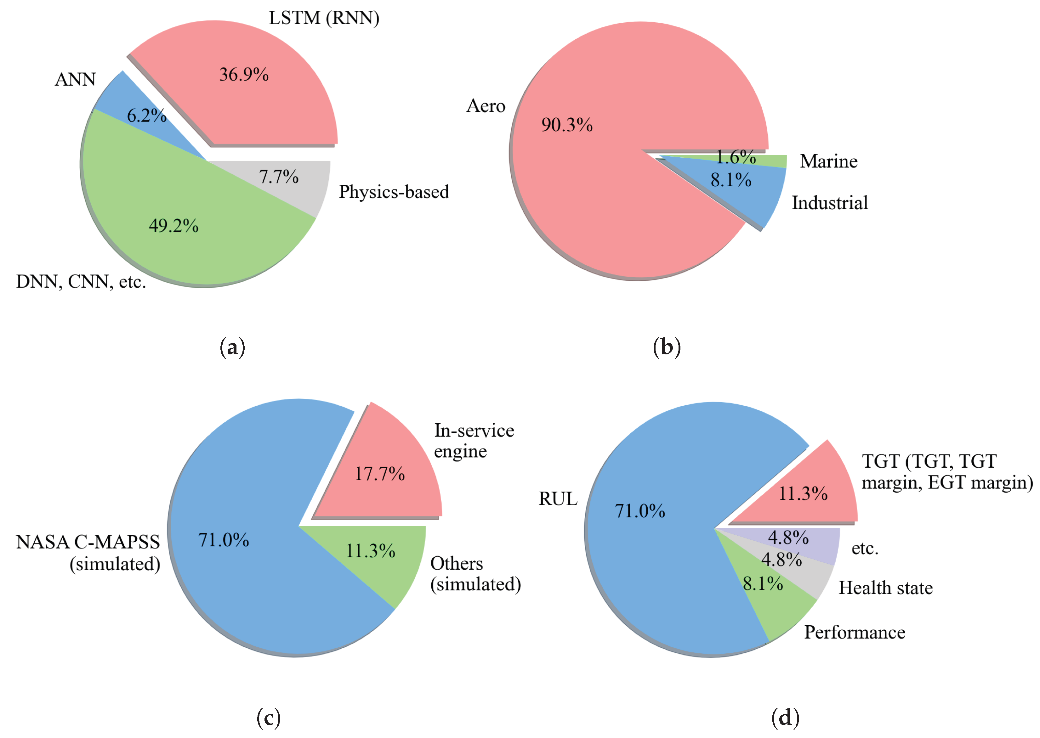
Figure 1. Surveys on previous works in the prognostics of gas turbine engines from the literature (2003–2023): (a) modeling approaches (artificial neural network, deep neural network, convolutional neural network, recurrent neural network, long short-term memory, etc.) and physics-based, (b) gas turbine type (Aero—aero engines, Marine—marine engines, Industrial—engines for power generation), (c) data source (NASA C-MAPSS, EHM data from in-service engine, other data from simulation), and (d) target variables (remaining useful life, turbine gas temperature, exhaust gas temperature, performance, health state of GT, etc.). This highlights the gap this study aims to fill.
Aerospace 12 00725 g001
Figure 2. Sampled EHM data of selected engines over their life cycles with maintenance records of major overhauls: (a) EHM data of a selected engine from turbofan family engine A, (b) EHM data of a selected engine from turbofan family engine B, (c) EHM data of a selected engine from turbofan family engine C. This illustrates pattern and incompleteness of in-service engine data.
Aerospace 12 00725 g002
Figure 3. Conventional train–test split method and data segmentation using engine maintenance intervals: (a) Conventional train–test split, (b) Data segmentation using engine maintenance intervals.
Aerospace 12 00725 g003
Figure 4. Applying detrending on the training dataset: (a) Original training dataset, (b) Detrended training dataset, (c) Trends of individual variables captured by polynomial fitting. Detrending helps the model to focus on underlying patterns.
Aerospace 12 00725 g004
Figure 5. Multi-engine-based large generalized model; Multi-engine-based large model is trained by utilizing datasets from multiple engines.
Aerospace 12 00725 g005
Figure 6. Module of long short-term memory (LSTM); Cell state (C) is the core of LSTM.
Aerospace 12 00725 g006
Figure 7. Box plot—Results of the linear regression algorithms on turbofan family engine A: (a) Approach I, (b) Train–test split.
Aerospace 12 00725 g007
Figure 8. Box plot—Results of the nonlinear regression algorithms on turbofan family engine A: (a) Approach I, (b) Train–test split.
Aerospace 12 00725 g008
Figure 9. Box plot—Results of the LSTM models on each turbofan family engine with segment-based training (Approaches I, II, and III), train–test split, and large model: (a) Turbofan family engine A, (b) Turbofan family engine B, (c) Turbofan family engine C.
Aerospace 12 00725 g009
Figure 10. Normalized prediction results of the LSTM model on turbofan family engine A, Approach I: (a) Example of prediction result near the mean value, (b) Example of outlier prediction result. Local deviations are observed with outliers from the models.
Aerospace 12 00725 g010
Figure 11. Result of uncertainty quantification using Delta method for multi-engine-based large generalized model: Turbofan family engine A. Most of target values lay within the uncertainty range.
Aerospace 12 00725 g011
Table 2. Summary of EHM data of fleets of turbofan family engines.
Turbofan Family Engine ATurbofan Family Engine BTurbofan Family Engine C
No. of enginesseveral hundredseveral hundredseveral hundred
No. of parameters<190<190<120
Flight envelopesTaxi-out, Take-off, Climb, Cruise, Taxi-in
Table 3. Selected sets of predictor variables for training ML model to predict TGT.
SymbolDescriptionUnitsSet 1 (10 Vars)Set 2 (9 Vars)Set 3 (8 Vars)Set 4 (7 Vars)Set 5 (6 Vars)Set 6 (5 Vars)Set 7 (4 Vars)Set 8 (3 Vars)
N1Low pressure spool speed%xxxxxxx
N2Intermediate pressure spool speed%xxxxxxxx
N3High pressure spool speed%xxxxxxxx
P25IPC delivery pressurepsixxxxx
P3HPC delivery pressurepsixxxxxx
P50Turbine exit pressurepsixxxx
T25IPC delivery temperatureCxxx
T3HPC delivery temperatureCxxxxxxxx
FFFuel flow ratelb/hxx
GWTAircraft gross weightlbsx
Table 4. Summary of TGT prediction using each set of predictor variables (Approach I, turbofan family engine A).
UnitsSet 1 (10 Vars)Set 2 (9 Vars)Set 3 (8 Vars)Set 4 (7 Vars)Set 5 (6 Vars)Set 6 (5 Vars)Set 7 (4 Vars)Set 8 (3 Vars)
mean RMSEC11.1612.4514.2914.1413.9614.0313.6516.03
median RMSEC9.039.5011.2311.2510.7110.710.0011.96
IQRC8.369.5212.4712.4511.7112.0711.9913.01
Q1C5.765.896.456.176.286.035.787.45
Q3C14.1215.4018.9218.6217.9918.1017.7720.47
max RMSEC41.0560.7960.1862.8259.4258.9263.0968.02
min RMSEC0.741.292.140.862.162.1662.431.67
outlier%6.306.804.744.125.365.575.576.19
Table 5. Segment-based ML model training approaches.
ApproachTraining DatasetTest DatasetHypothesis
I
(one-to-many)
segment 1 onlysegment 2 N Segment 1 represents the deterioration of
a new engine, which can be used for generic
training data for the rest of the service period
II
(many-to-many)
segment 1 ( N 1 ) segment NThe progressively accumulated data will provide
all the historical deterioration characteristics for
the ML model so that it can make more accurate predictions
III
(one-to-one)
segment N 1 segment NOnly the EHM data of the previous service period is
valid to represent the latest condition so that it
can represent the deterioration characteristics
Train–test split80%20%Conventional ML model training method,
use 80% of the available data of each engine for training,
test the trained model on the remaining 20% of the data for each engine
Table 6. Linear and nonlinear regression algorithms.
Linear AlgorithmsNonlinear Algorithms
AlgorithmAbbr.ReferenceAlgorithmAbbr.Reference
Linearlrn/aK-nearest neighborsknn[43]
Lassolasso[44]Decision treecart[45]
Ridgeridge[46]Extra treeet[47]
Elastic neten[48]Support vectorsvmr[49]
Huberhuber[50]Adaboostada[51]
Lasso larslassol[52]Baggingbag[53]
Passive aggressivepa[54]Random forestrf[55]
Stochastic gradient decentsgd[56]Gradient boostinggbm[57]
Table 7. Hyperparameters for LSTM model.
HyperparameterParameter Set
No. of layers1
Units10
Epochs100, 200, 500, 1000
Batch size32, 64, 128
Learning rate0.001
OptimizerAdam
Loss functionmse
Table 8. Prediction results of linear, nonlinear regression algorithms, and LSTM on turbofan family engine A.
LinearNonlinearLSTM
Approach lr lasso lassol huber en pa ridge sgd ada bag cart et extra gbm knn rf svmr -
IMean3.116.276.263.023.713.913.023.276.214.475.534.155.734.285.874.473.174.14
Median2.445.605.642.443.313.042.412.824.673.474.433.244.563.384.483.452.522.86
Max.39.0330.4530.4533.1830.4381.0334.1030.4936.4430.5730.5730.5130.9530.4731.3230.5536.2830.52
Min.0.000.000.000.000.000.030.000.000.940.250.070.060.130.160.290.040.040.00
IQR1.023.683.600.921.001.640.960.992.371.762.121.482.191.513.361.821.031.66
Outlier8.581.761.949.587.229.137.6610.0712.1011.6912.5813.6910.2012.458.6212.0610.4712.78
IIMean3.116.196.223.073.704.113.063.176.214.065.293.835.313.945.134.073.333.88
Median2.495.755.812.483.353.282.462.784.493.314.273.164.393.294.093.332.562.92
Max.39.0330.4530.4533.1830.4348.3234.1030.5083.6430.5749.9430.5033.2230.4631.3230.5630.4132.79
Min.0.000.000.000.010.000.060.000.010.780.180.070.370.140.550.960.330.130.17
IQR1.153.043.131.121.041.951.040.881.921.532.071.371.851.372.291.521.201.60
Outlier8.272.402.179.357.087.428.419.6315.978.7510.0410.0910.608.678.789.1712.4710.52
IIIMean3.236.326.323.133.754.253.093.276.314.335.354.035.444.165.524.313.214.05
Median2.415.825.822.413.332.962.392.774.573.374.243.174.343.304.223.322.512.83
Max.87.6430.4530.4583.7630.43178.7451.9930.5078.9340.7540.7540.7540.7540.7540.7540.7530.4158.55
Min.0.000.000.000.020.000.010.000.000.200.140.120.010.260.290.190.090.000.05
IQR0.963.373.350.931.041.470.940.842.071.641.811.391.831.412.561.631.031.52
Outlier8.902.212.169.517.2210.077.7111.2913.6311.0911.7612.0111.6010.999.7210.8512.1611.96
Train–testMean3.116.596.613.133.974.423.123.396.124.095.363.925.303.955.034.113.323.39
Median2.496.116.102.483.453.302.492.804.483.394.323.224.453.334.203.402.602.72
Max.39.6439.5139.5139.7439.7839.9639.7739.9952.2740.1047.5740.2340.8040.1441.6740.0439.8340.19
Min.0.891.991.980.901.490.970.851.191.891.602.481.532.581.522.321.600.891.00
IQR1.283.263.281.271.072.251.280.931.961.381.561.321.471.171.661.401.311.31
Outlier6.283.493.546.947.677.906.428.7111.357.489.277.827.427.919.547.587.587.05
Note: All values are in [°C] except Outlier, which is in [%]; Mean: Mean RMSE, Median: Median RMSE, Max: Maximum RMSE, Min: Minimum RMSE, IQR: Interquartile range; Minimum values from linear and nonlinear algorithms are highlighted in bold.
Table 9. Prediction results of the LSTM models on each turbofan family engine.
Approach IApproach IIApproach IIITrain–Test SplitLarge Model
Turbofan family engine AMean4.143.884.053.393.44
Median2.862.922.832.722.94
Max.30.5232.7858.5540.1930.48
Min.0.000.170.051.000.66
IQR1.661.601.521.310.94
Outlier12.7810.5211.967.059.47
Turbofan family engine BMean5.504.864.634.413.38
Median3.602.902.792.503.28
Max.24.1024.2423.45106.6010.72
Min.0.110.030.021.582.11
IQR4.503.373.251.480.47
Outlier7.269.839.8310.715.56
Turbofan family engine CMean4.454.904.774.555.48
Median3.543.883.194.004.88
Max.30.0651.6058.5719.3623.92
Min.0.110.120.431.231.72
IQR2.392.332.262.941.64
Outlier7.055.6310.395.658.19
Note: All values are in [°C] except Outlier, which is in [%]; Mean: Mean RMSE, Median: Median RMSE, Max: Maximum RMSE, Min: Minimum RMSE, IQR: Interquartile range; Minimum values are highlighted in bold.
Table 10. Normalized amount of data (i.e., engine cycles) used for model training and testing.
DatasetApproach IApproach IIApproach IIITrain–Test SplitLarge Model
Turbofan family engine ATraining0.650.950.701.00277.40
Test0.520.520.520.280.52
Turbofan family engine BTraining0.811.080.681.00116.68
Test0.440.440.440.280.44
Turbofan family engine CTraining0.350.780.451.0044.25
Test0.520.520.520.280.52
Table 11. Results of uncertainty quantification using Delta method for multi-engine-based large generalized models.
CWCMAENMPIWPICPMPIWStdAEStdPIW
Turbofan family engine A30.992.2212.1999.6630.991.870.00
Turbofan family engine B39.352.545.5692.5212.072.070.00
Turbofan family engine C29.193.9910.4598.5329.192.860.00
Note: All metrics represent median values except PICP, which is the mean value; All values are in [C], except NMPIW and PICP, which are in [%]; StdAE and StdPIW represent standard deviation of absolute error and prediction interval width.
Disclaimer/Publisher’s Note: The statements, opinions and data contained in all publications are solely those of the individual author(s) and contributor(s) and not of MDPI and/or the editor(s). MDPI and/or the editor(s) disclaim responsibility for any injury to people or property resulting from any ideas, methods, instructions or products referred to in the content.