Abstract
The gradual integration of Manned–Unmanned Teaming (MUM-T) is gaining increasing significance. An intriguing feature is the ability to do relative estimation solely through the use of the INS/GPS system. However, in certain environments, such as GNSS-denied areas, this method may lack the necessary accuracy and reliability to successfully execute autonomous formation flight. In order to achieve autonomous formation flight, we are conducting an initial investigation into the development of a relative estimator and control laws for MUM-T. Our proposal involves the use of a quaternion-based relative state estimator to combine GPS and INS sensor data from each UAV with vision pose estimation of the remote carrier obtained from the fighter. The technique has been validated through simulated findings, which paved the way for the experiments explained in the paper.
1. Introduction
Manned–Unmanned Teaming (MUM-T), Figure 1, is the cooperative interaction between manned and unmanned aircraft, in order to improve the overall capabilities of a mission. This concept involves the collaboration between human-operated aircraft and unmanned aerial vehicles (UAVs) or remote carriers. The objective is to exploit the advantages of both types of aircraft in order to accomplish operations that are more efficient and adaptable.
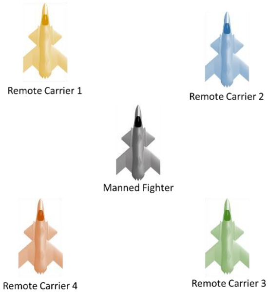
Figure 1.
MUM-T formation.
The utilization of this cooperative strategy is extensively utilized in military contexts, where MUM-T significantly improves the efficiency and efficacy of surveillance, reconnaissance, and other mission categories. The integration of piloted and unpiloted platforms optimizes the advantages of each, enhancing the overall effectiveness and flexibility of air warfare tactics.
MUM-T enables seamless communication and coordination. MUM-T facilitates uninterrupted communication and coordination between manned and unmanned platforms, enabling them to exchange information, carry out complementary activities, and improve situational awareness. Piloted aircraft can gain advantages from the supplementary functionalities of unmanned carriers, including enhanced range, prolonged endurance, and the capacity to enter hazardous locations without endangering human pilots. Unmanned vehicles can utilize the knowledge and decision-making skills of human pilots.
MUM-T refers to a continuous flight where manned and unmanned aircraft fly closely together. Close-formation flying poses a challenge that requires an accurate estimation of the relative state between the fighter aircraft and the remote carriers, as well as a reliable formation guidance system that utilizes this estimated relative state. A straightforward approach to determine the relative placement is comparing the GPS coordinates of the fighter aircraft (manned) with those of the remote carriers. This technique is valuable for precise formation flight in situations when there is a significant distance between aircraft. The precision of this method is measured in meters, which may not be sufficient for flying in close formation.
However, it is also effective in environments where Global Navigation Satellite System signals are not available. Furthermore, a source of perturbations to consider is the temporal synchronization discrepancy that arises when comparing data between unmanned aerial vehicles (UAVs). This error is amplified by elevated horizontal vehicle motion and data losses.
In comparison to previous research efforts, the present work distinguishes itself by addressing relative navigation and control within a modular and platform-agnostic MUM-T framework. While many studies have focused on hardware-specific implementations, operator-centric interfaces, or platform-dependent estimation algorithms, few have proposed a sensor fusion and control architecture that can generalize across vehicle types and mission profiles. This scalability is critical to enable reliable coordination between heterogeneous unmanned and manned aerial systems operating under GNSS-degraded conditions, latency, and environmental uncertainty.
To attain the accuracy required for close-formation flight—especially in contested airspaces or autonomous refueling scenarios—it is necessary to complement visual data with inertial and absolute references. Vision-only techniques such as active contours [1], silhouette tracking [2], and neural network-based processing [3] have shown promise in controlled environments. Others, like camera-based geometric localization [4,5], attempt to reconstruct a position directly from passive vision. However, these methods are prone to occlusion, mismatching, clutter, and lighting variation, limiting their operational robustness.
For this reason, modern vision-based navigation systems in MUM-T increasingly rely on sensor fusion, combining visual markers with data from inertial measurement units (IMUs), magnetometers, barometric altimeters, and GNSS receivers. Systems such as those proposed for autonomous aerial refueling [6,7] or collaborative UAV tracking [8,9] have shown that multi-source fusion provides the reliability and fault-tolerance necessary for precise relative estimation in complex scenarios.
While the estimation framework forms the core of the proposed solution, it is equally important to position this contribution within the broader MUM-T systems literature.
A valuable system-level taxonomy of MUM-T configurations is presented in [10], focusing on AI and interoperability protocols such as STANAG 4586. A detailed historical evolution of MUM-T in U.S. Army aviation is presented in [10], documenting the progression of Levels of Interoperability (LOI) with platforms like Apache and Hunter. These contributions help contextualize current architectural needs, but do not tackle the estimation problem directly.
Kim and Kim introduce a helicopter–UAV simulation platform integrating PX4-based drones with a full-scale simulator in Unreal Engine [10]. Their system excels in HMI experimentation, offering tactile and immersive feedback loops for operator-in-the-loop testing. However, it does not include estimation modules or GNSS-degraded capability evaluation.
A timeline-based task assignment planner that enables multi-level delegation of UAV tasks to the pilot is presented in [11]. Their planner is tested with military pilots in the IFS Jet simulator and proves effective for mission-level decision flow. Later, Ref. [12] extend this approach by incorporating mental resource models—specifically the capacity model and Wicken’s multiple resource theory—into task allocation logic. By anticipating pilot workload, their planning system schedules UAV tasks to avoid cognitive overload, thus preserving performance.
In more adversarial contexts, other works have tackled autonomous maneuverings and control. Ramírez López and Żbikowski [13] simulate autonomous decision-making in UCAV dogfighting, modeling maneuvers as a game-theoretic problem space. Similarly, Huang et al. [14] propose a Bayesian inference-based optimization framework using moving horizon control for combat trajectory selection, showing improved survivability under dynamic threats.
An autonomy balancing in MUM-T swarm engagements is presented in [15]. Their RESCHU-SA simulation integrates physiological feedback (heart rate and posture) to adjust autonomy levels based on operator stress, showing how mixed-initiative control improves mission performance. This perspective of dynamic autonomy assignment complements our work’s focus on robust estimation under variable data availability.
Human–machine interface (HMI) studies have also shown relevant results; the authors of [16] compare voice, touch, and multimodal inputs for UAV control in high-stress scenarios, concluding that touch-based input consistently outperforms others in terms of reliability and operator preference. The authors of [17] present the Hyper-Enabled Operator (HEO) framework, emphasizing cognitive load reduction and seamless HMI design as critical enablers for effective MUM-T command.
This paper proposes a novel relative estimation and control framework for Manned–Unmanned Teaming (MUM-T), specifically designed to enable autonomous close-formation flights in dynamic and complex operational scenarios. The core objectives of this work are threefold: (1) to develop a quaternion-based relative state estimator that integrates data from GPS, Inertial Navigation Systems (INSs), and vision-based pose estimation to enhance accuracy and robustness; (2) to validate the proposed framework through comprehensive simulations and initial experimental trials, demonstrating its feasibility in real-world applications; and (3) to effectively address challenges such as temporal synchronization discrepancies, GNSS degradation, vision dropouts, and sensor noise by employing an Unscented Kalman Filter (UKF), which is known for its superior performance in nonlinear estimation problems without requiring Jacobian computations.
Unlike the Extended Kalman Filter (EKF), which requires the derivation and linearization of Jacobians, the UKF uses a deterministic sampling method (sigma points) to propagate uncertainty through nonlinear transformations. This not only improves estimation accuracy through a second-order approximation [18,19] but also increases numerical stability and resilience to poor initialization—key in scenarios where GPS may be intermittent and visual markers may briefly disappear.
In this work, the UKF is applied in two distinct layers:
- First, an onboard AHRS (Attitude and Heading Reference System) fuses GPS, IMU, magnetometer, and barometer data to maintain stable state estimation in each UAV.
- Second, a relative state estimator on the leader or tanker aircraft uses visual PnP-based measurements (e.g., using POSIT [20]) combined with the state vectors of both vehicles to infer relative pose. The POSIT (Pose from Orthography and Scaling with Iterations) algorithm was employed to estimate the three-dimensional pose of known rigid objects from single monocular images. This method assumes that the intrinsic parameters of the camera are known and relies on a set of 2D-3D correspondences between image features and predefined object landmarks. POSIT initially approximates the object pose using a scaled orthographic projection, which simplifies the computation. It then iteratively refines the solution by updating the estimated depths of the 3D points, progressively converging toward a more accurate perspective pose. Due to its computational efficiency and robustness in real-time scenarios, POSIT was particularly suitable for the visual tracking and spatial estimation tasks addressed in this work.
A well-documented limitation of the UKF in attitude representation is that quaternion-based filtering can yield non-unit quaternions when averaging sigma points. To address this, the present work implements Generalized Rodrigues Parameters (GRPs) for attitude error representation, following the approach of Crassidis & Markley [19], where a three-component GRP vector is used within the UKF framework. This method preserves quaternion normalization, reduces covariance size, and has been shown to outperform conventional EKF in scenarios with large initialization errors.
The use of relative navigation techniques between aerial vehicles has been previously explored by Fosbury and Crassidis [21], who investigated the integration of inertial and GPS data for estimating relative position and velocity in formation flight. Their work emphasized the importance of accurate time synchronization and sensor alignment, particularly in distributed systems where each vehicle independently estimates its own state. While their estimator was primarily based on Extended Kalman Filter (EKF) formulations, the foundational insights regarding the coupling of inertial and GNSS measurements for inter-vehicle navigation directly inform the architecture presented in this work. In contrast, the proposed system builds upon these principles by incorporating visual observations and switching to a quaternion-based Unscented Kalman Filter (UKF) with GRP-based attitude error representation, thereby improving estimation consistency and robustness under nonlinear conditions.
This approach builds upon past work in visual navigation and aerial refueling [7,22,23,24,25], where both relative state and estimation frameworks were evaluated under dynamic, nonlinear flight conditions. However, unlike previous implementations that often relied on tightly coupled hardware platforms and custom estimation logic, our approach prioritizes modularity and abstraction, enabling deployment across a range of airframes and mission contexts.
The evolution of Manned–Unmanned Teaming (MUM-T) is intrinsically tied to advancements in distributed intelligence and cooperative control, particularly those inspired by swarm robotics and network-centric warfare. Foundational work by Beni introduced the concept of swarm intelligence as a form of self-organized behavior in distributed systems without centralized control, which later evolved into the framework of swarm robotics as applied to collective mobile agents like UAVs [26,27]. This paradigm has greatly influenced the development of cooperative robotic systems, where simple agents interact locally to produce complex, emergent behavior [28,29].
MUM-T systems leverage such decentralized architectures to increase flexibility, resilience, and mission efficiency. In this context, cooperative control strategies allow unmanned aerial systems (UASs) to dynamically share tasks, react to environmental changes, and support manned platforms without requiring explicit micromanagement [30]. Architectures enabling these behaviors are often aligned with principles of network-centric warfare (NCW), where connectivity and information superiority become key enablers of operational effectiveness [31,32,33], further emphasizing the need for scalable command and control mechanisms capable of orchestrating large UAV swarms in adversarial scenarios, as demonstrated in the 50 vs. 50 live-fly competition.
A critical aspect in the deployment of MUM-T systems lies in airborne communication networks, where small UAVs form dynamic links to ensure robust coordination with manned assets [34]. These networks support varying degrees of autonomy and delegation, ranging from basic Level 1 ISR feed relay to Level 5 full mission autonomy [35]. The implementation of such multi-level delegation schemes has been explored in recent operational planning tools that use timeline-based tasking and mixed-initiative interfaces [36].
From a practical standpoint, modern MUM-T concepts aim to transition from isolated mission execution toward robotic autonomous systems that seamlessly collaborate with manned platforms in contested environments. Capstone studies and field demonstrations have validated the utility of this teaming, particularly in ISR, targeting, and refueling roles [37]. For instance, autonomous aerial refueling tasks now benefit from multi-sensor fusion strategies, such as vision/GPS integration through Extended Kalman Filters (EKFs), enabling precise relative navigation during cooperative engagements [38].
Ultimately, the convergence of swarm theory, cooperative autonomy, robust C2 architectures, and applied mission planning underpins the growing maturity of MUM-T systems. These developments not only expand the tactical envelope of unmanned platforms but also redefine the role of human operators in future joint operations.
Additionally, the proposed system is architected with modularity and platform agnosticism in mind. The relative navigation and control framework is intentionally designed not to be tightly coupled to any specific aircraft model or sensor configuration. Instead, it supports generalization across heterogeneous aerial platforms with different dynamic characteristics. This abstraction of vehicle-specific dynamics enables broader applicability of the system, facilitating its integration into collaborative MUM-T operations across diverse mission profiles. To further enhance its flexibility, the system has been implemented in a way that allows it to function as a high-level control layer on top of standard autopilot systems commonly used in UAVs, such as ArduPilot in this case, as can be seen in Figure 2. This approach simplifies integration efforts and ensures compatibility with existing flight control architectures.
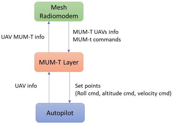
Figure 2.
High-level architecture.
Finally, an extensive simulation environment has been developed to rigorously evaluate the performance of the framework under a range of realistic conditions, including GNSS outages, visual occlusion, and maneuvering flight. These simulation results pave the way for future ground-based and in-flight testing campaigns, with the ultimate goal of deploying the proposed MUM-T system in operational environments requiring precise, resilient, and scalable formation control capabilities.
In summary, the proposed system leverages advances in UKF estimation, GRP attitude error representation, and multi-sensor fusion to achieve sub-meter accurate relative navigation in formation flight and GNSS-degraded environments. It does so while maintaining modularity across airframe types and being robust to initialization errors and visual signal dropouts. When compared to previous works—whether they emphasize control, planning, or human–machine interaction—this paper uniquely integrates a resilient, platform-agnostic estimation framework directly linked to robust formation flight control for MUM-T missions.
The remainder of this paper is organized as follows: Section 2 provides a detailed problem formulation, including the design of the relative estimation algorithm and its mathematical foundations. Section 2.3 describes the implementation of the vision system. Section 3 focuses on the guidance and control strategies for maintaining formation flight configurations. Section 4 presents simulation results, evaluating the performance of the proposed framework in diverse scenarios. Section 5 outlines experimental setups and findings, highlighting real-world applicability. Finally, Section 6 concludes the paper, summarizing key achievements and identifying directions for future research.
2. Relative Estimation in Remote Carrier Frame
This section provides a comprehensive explanation of the relative estimation algorithm. Initially, a comprehensive evaluation of the state estimation of each individual UAV should be conducted using a UKF. Following this, the algorithm can be further expanded to predict the relative position and orientation between the remote carriers and the fighter aircraft. Next, we will provide an explanation of the additional eyesight metrics that will be included.
2.1. Individual Remote Carrier UAV Stare Estimation
Following the approach outlined in [11], a state estimator based on the Unscented Kalman Filter (UKF) is employed for each UAV. The individual state estimation, denoted as x, is determined by fusing data from multiple onboard sensors [7]. This estimation process is divided into two key stages: prediction and observation. During the prediction stage, the UAV’s dynamic model forecasts the state vector for the next time step. The inputs for this stage include angular rates from the three-axis gyroscopes and linear accelerations from the three-axis accelerometer, both measured in the body axis.
Figure 3 has been updated to explicitly show that the Prediction block uses IMU measurements (gyroscopes and accelerometers), while the Observation block incorporates GPS, magnetometer, and barometer readings. This modification improves the clarity of the sensor fusion process within the UKF structure.
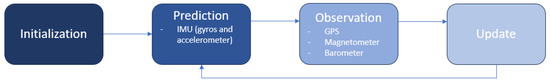
Figure 3.
UKF flowchart.
In the observation stage, sensor measurements such as GPS data, three-axis magnetometer readings, and barometer outputs are incorporated to refine the predicted state estimate. This two-stage process ensures accurate state estimation by continuously updating the UAV’s position, velocity, and orientation based on a combination of predicted dynamics and real-time sensor observations.
The position , and velocity are expressed in the North–East–Down (NED) navigation frame, which is defined as a local Earth-fixed frame tangent to the geoid at the geodetic reference of the ground control station. Although not strictly inertial, the NED frame is treated as quasi-inertial under the small-area and short-time assumptions commonly accepted in UAV applications. Accordingly, the coordinate components X, Y, and Z refer, respectively, to the north, east, and down axes of this frame. This convention has been adopted throughout the estimation process to ensure consistency between the dynamic model and measurement updates. The quaternion represents the aircraft’s attitude and is used to construct the rotation matrix , which is utilized to convert from the body frame to the navigation frame; the (NED) frame is constructed using a standard 3-2-1 (yaw–pitch–roll) Euler angle sequence. That is, the matrix applies consecutive rotations around the Z (yaw), Y (pitch), and X (roll) axes. This convention is widely used in aerospace applications due to its intuitive physical interpretation and compatibility with IMU measurements. and are the accelerometer and gyroscope bias. The precise definition of , along with other inertial mechanization equations, and a comprehensive derivation of the INS mechanization equations can be found in reference [39].
Although Euler angles are referenced in the initial attitude computation for interpretability, the rotation matrix is computed directly from the unit quaternion using the standard quaternion-to-direction cosine matrix (DCM) transformation. This approach maintains full consistency with the quaternion-based attitude representation in the UKF. The quaternion representation avoids singularities and guarantees numerical stability during state propagation and updates. Euler angles and their sequence (ZYX—yaw, pitch, roll) are used exclusively during initialization, and their definitions have now been clarified accordingly.
The rotation matrix is obtained from the unit quaternion as follows:
2.1.1. Initialization
represents the initial state of vector P and is calculated using the raw GPS measurements in the geodetic frame; the initial velocity is an average of the raw GPS velocity; and ω are assumed to be zero, where ω is the angular rate. The initial Euler orientation, , , and , is calculated using the accelerometer measurements , where are the accelerations in the three body axes and magnetometer measurements , where are the magnetic fields in the three body axes, as shown in Equation (4) to Equation (6), and is the magnetic declination.
2.1.2. Prediction
The vehicle state is propagated by the inputs, u, in Equation (7), which are the accelerometer measurements gyro measurements , and mean of the Gaussian white noise processes that govern and ω. The process noise covariance Q is provided in Equation (8).
The inputs, u, consist of the angular rates obtained from the three-axis gyroscopes and the acceleration obtained from the three-axis accelerometer in the body axis, which is completed with the necessary empty matrices for consistency.
In Equation (6), each diagonal element represents the variance of a specific noise source associated with the system’s state dynamics. The variables are described as follows. represents the variance of the accelerometer bias noise. This term models the uncertainty related to the drift or slow variation in the accelerometer bias over time, which is critical for maintaining long-term accuracy in inertial navigation systems. denotes the variance of the gyroscope bias noise in the body reference frame. This parameter accounts for the uncertainty due to the drift in the gyroscope bias, which can significantly affect the precision of attitude estimation. corresponds to the variance of the body-frame acceleration noise. It models the uncertainty associated with the actual acceleration of the body, which may arise from unmodeled dynamics, external disturbances, or measurement errors. refers to the variance of the body-frame angular velocity noise. This term captures the uncertainty in the actual angular velocity of the body, which can be influenced by dynamic changes not accounted for in the model. represents the variance of the general process noise related to angular velocity. This parameter models random disturbances or unmodeled noise affecting the angular velocity estimation, typically treated as white noise.
The downside to a quaternion attitude parametrization in a UKF is that a unit norm cannot be guaranteed during propagation. To overcome this, a method described in [19] was implemented. The Unscented Filter for nonlinear systems employs a meticulously chosen set of sample points to more precisely represent the probability distribution compared to the linearization of the standard Extended Kalman Filter, resulting in expedited convergence from erroneous initial conditions in attitude estimation issues. The filter formulation relies on typical attitude-vector measurements utilizing a gyro-based model for attitude propagation. The global attitude parameterization is represented by a quaternion, but a generalized three-dimensional attitude representation is employed to delineate the local attitude error. A multiplicative quaternion-error method is formulated from the local attitude error, ensuring the preservation of quaternion normalization within the filter.
The Unscented Kalman Filter (UKF) was selected over the Extended Kalman Filter (EKF) due to its improved robustness in the presence of large initial attitude errors and nonlinearities in rotational motion. Unlike the EKF, the UKF does not rely on local linearization and instead uses a deterministic sampling approach to propagate the mean and covariance through nonlinear transformations. This leads to better estimation accuracy, particularly in attitude estimation problems involving high angular rates or poor initial conditions. Several works have reported these advantages, including [19,40].
In terms of computational performance, the UKF remains feasible for real-time execution onboard aerial platforms. For instance, ref. [19] demonstrated that the UKF could be implemented efficiently for spacecraft attitude estimation with update rates exceeding 50 Hz using state vectors of similar size to those used in this work. More recent benchmarking studies, such as [41], report average execution times below 1 ms per cycle for UKF implementations with 15–20 state variables on embedded platforms, including ARM Cortex-M7 and STM32H7 microcontrollers. Although the UKF is more computationally demanding than the EKF due to the propagation of sigma points, this overhead is offset by its superior numerical stability and estimation accuracy in nonlinear attitude estimation problems.
For state propagation, the inertial navigation mechanization equations given in Equation (9) are used.
where is the position vector in the NED (North–East–Down) navigation frame, V is the velocity vector in the NED frame, q is the unit quaternion representing the orientation of the body frame with respect to NED, is the gyro bias, and is the accelerometer bias. In the notation used throughout this work, a dot above a variable denotes its time derivative, that is, the rate of change in the variable with respect to time. This convention is standard in dynamic systems modeling and is applied consistently to represent the evolution of state variables such as position, velocity, attitude, and sensor biases.
is the direction cosine matrix (rotation matrix from navigation to body frame), is the corrected acceleration measured in body frame, is the Earth rotation rate expressed in the NED frame, is the rotation of the navigation frame with respect to inertial in the NED frame, and is the gravitational acceleration vector in the NED frame. The notation represents the quaternion derivative induced by the corrected angular velocity . Here, is a 4 × 4 quaternion propagation matrix built from the bias-compensated angular rate vector. This matrix enables quaternion propagation within the UKF without requiring explicit trigonometric operations, maintaining consistency with the continuous-time kinematic model. is the gyroscope bias noise (process noise), and is the accelerometer bias noise (process noise).
Here, q is replaced with a three-dimensional Generalized Rodrigues Parameter (GRP) vector, from to . represents attitude error and is initialized to zero. This formulation has the added benefit of reducing the state dimensionality procedure. GRP is a compact representation of a rigid body’s orientation in three-dimensional space, derived from the unit quaternion.
Although not shown in Equation (1), the state transition model internally propagates the effect of angular velocity ω from gyroscope measurements, which is included in the input vector u. In Equation (9), attitude propagation is driven by these angular rates, ensuring that rotational dynamics are fully captured.
The unscented transform can now occur by first concatenating and u and their respective covariance, P and Q. The sigma points, , can now be formed by perturbing by the root of scaled by K. K is chosen such that , where is the dimension of . We set to 3 as per [18].
To represent attitude errors within the UKF framework, we employ the Generalized Rodrigues Parameters (GRPs), which offer a minimal three-dimensional representation suitable for small angular deviations.
This choice is motivated by the fact that unit quaternions lie on a nonlinear manifold and cannot be directly perturbed or averaged in a Euclidean sense, which is required by the Unscented Kalman Filter. GRPs provide a minimal, three-dimensional representation of attitude error in the tangent space of the quaternion manifold, enabling additive updates and linear error modeling. Although the full quaternion is still maintained as part of the state vector, the use of GRPs during the sigma point transformation avoids introducing constraints or renormalization steps. This approach is consistent with [5] and other aerospace UKF implementations and provides a balance between computational efficiency and numerical robustness. Therefore, the rationale is not to reduce the number of estimated states, but to enable a minimal and well-defined representation of rotational error during the filter update.
Rather than estimating only the imaginary components of the quaternion and reconstructing the scalar part via the unit-norm constraint, we adopt a more robust approach. Specifically, the full quaternion is estimated, and attitude error corrections are applied through multiplicative updates using the relation:
This formulation guarantees normalization and numerical stability without introducing discontinuities or ambiguity in the quaternion space. The GRP representation allows for linear error modeling during the filter update, while the quaternion structure is preserved throughout the estimation process.
It should be noted that the GRP-based representation does not correct any pre-existing normalization errors in the input quaternion. If the original measurement quaternion is not unit-norm due to sensor error or noise, transforming it into GRP space does not inherently remove this deviation. Instead, the GRP formulation provides a singularity-free, minimal parameterization of small attitude deviations suitable for additive updates in the UKF. Therefore, quaternion normalization is enforced separately after each update to maintain consistency and ensure stable propagation.
Before can be propagated, each must be converted back to a quaternion parametrization by first calculating the local error quaternion, , using Equation (14).
and f are scale factors. We chose as per [19]. The sigma point quaternions, , are then calculated by perturbing the current estimate by the attitude error . The symbol denotes quaternion multiplication.
Each of the sigma points are now transformed by the inertial navigation mechanization equations given in Equation (9). is the Earth gravity vector in the navigation frame and is the rotation of Earth in the navigation frame, as defined in [39]. We assume that the navigation frame is fixed and thus is a vector of zeros. and are the IMU accelerometer and gyro varying bias, is the Earth gravity vector in the navigation frame, and is the rotation of Earth in the navigation frame [39], and it is assumed that the navigation frame is fixed; therefore, is a zero vector. and are the biases of the accelerometer and gyroscope, and sensor are defined as white noise, where and are zero-mean Gaussian random variables. and are the bias- and noise-corrected imu measurements. and are the accelerometer and gyro measurement noise terms. Gyro measurements are corrected by the Earth’s rotation.
P and V are propagated with a first-order Euler integration whereas the discretized quaternion propagation is given by Equation (9). The skew matrix, is composed of bias-corrected gyro measurements and ∆t is the propagation timestep.
where s is small-angle approximation in rotational motion.
I is the identity matrix, and η determines the convergence speed of the numerical error. For stability, [42]. A full derivation of the INS mechanization equations can be found in [39]. Before the predicted mean and covariance can be calculated, the propagated quaternions, , must be converted back to δp using Equation (23).
The UKF predicted mean and covariance can now be calculated using Equations (24) and (25) as per [19].
where the a priori state estimate at time k + 1, denoted as is computed as a weighted average of the propagated sigma points. The corresponding equation is given by Equation (24) in this formulation:
- represents the central sigma point, typically corresponding to the mean of the prior distribution.
- for i = 1,2,…, are the sigma points generated by the unscented transformation, symmetrically distributed around the mean.
- The upper bound of the summation, , reflects the number of sigma points derived from a state-input augmented vector of dimension . This includes both the system state x and any additional components such as process noise or control inputs u that are incorporated into the augmented state vector.
The scalar λ is a scaling parameter derived from the UKF’s tuning coefficients (typically involving α, κ, and β) and ensures appropriate dispersion of the sigma points. The weights associated with the sigma points are normalized such that the resulting estimate remains unbiased and captures the second-order statistics of the system’s nonlinear transformation.
This formulation ensures that the mean estimate accounts for the nonlinear propagation of uncertainty, which is especially critical in systems where linearization would lead to significant approximation errors.
The a priori error covariance matrix in the Unscented Kalman Filter (UKF), denoted as , is computed based on the statistical dispersion of the sigma points around the predicted mean. The corresponding expression is
In this formulation:
- is the central sigma point.
- for i = 1, 2,…, are the additional sigma points generated through the unscented transformation from the augmented state.
- represents the predicted mean of the state at time k + 1.
- The term reflects the number of sigma points, where denotes the dimension of the augmented state vector, including the state and possibly control inputs and noise terms.
- λ is a UKF scaling parameter that determines the weight of the central sigma point.
- The summation term computes the contribution of the remaining sigma points to the covariance.
This formulation ensures that the covariance accounts for the full second-order nonlinear effects in the propagation of uncertainty. The resulting matrix captures the predicted uncertainty in the state estimation and serves as a fundamental component for the subsequent update step in the UKF.
2.1.3. Observation
In the state observation phase, GPS, atmospheric, and magnetic measurements are used to observe and update the state estimate. First, the expected observations, , are calculated using as shown in Equation (26). This uses the propagated quaternions rather than GRP parametrization, where h represents the measurement model in the estimation process.
The different sensor sampling rates have to be taken into account, thereby occurring sequentially, and is used when GPS measurement is available, whereas is taken into account when magnetometer and pressure observations are available.
where is the GPS-based position estimation, is the GPS-based velocity estimation, is the predicted position, is the rotation matrix from the body frame to the navigation frame, is the position of the GPS antenna relative to the center of gravity, and are the measurement noise terms for the GPS position and velocity, respectively. is the predicted velocity, and is the skew–symmetric matrix of angular velocity.
The measurement update step handles two distinct sensor update rates. GPS measurements (position and velocity) are received at a lower rate (5 Hz), while all other sensors—namely the IMU, magnetometer, and barometer, are processed at a higher, common rate (50 Hz). To support this configuration, the UKF performs measurement updates asynchronously, based on the availability of new data from each group.
Equation (28) represents the general form of the measurement update and is applied to all sensor types. The function h(x) and the associated measurement noise covariance R are adapted depending on which sensor group is currently being processed. Thus, Equation (28) also applies to the magnetometer and barometer measurements, with specific models embedded in the general update structure.
Where is the predicted measurement vector at time step based on the predicted state , is the initial height, and Z is the vertical distance. The elements , , and represent the orientation of the body frame relative to the reference frame. The combination forms part of the quaternion-to-Euler angle transformation, specifically extracting the pitch or roll angle. The expression calculates a yaw Euler angle from quaternion components. Finally, determines the predicted dynamic pressure, where represents the standard dynamic pressure formula, representing the pressure exerted by the moving air around the UAV.
and are the measurement noise terms of the pressure altitude and the heading. The raw data from the sensor must undergo preprocessing before being used in the previously stated observation models. The GPS readings are initially recorded in the geodetic frame and then transformed into the navigation frame using the specified transformation method [39]. Then, heading is calculated from the observed magnetic vector, by first de-rotating through roll, ϕ, and pitch, θ, using Equations (29) and (30) and then calculating using Equation (31). A magnetic declination correction accounts for the local difference in magnetics and true north.
The altitude above mean sea level (MSL), , is now calculated using the atmospheric pressure. First, the pressure at MSL, , is estimated using Equation (32) where is the initial pressure and is the initial MSL height, as observed by the GPS. Finally, is determined using Equation (33) with L, , M, and R provided in Table 1.

Table 1.
ISA constants.
Equations (32) and (33) are derived from the International Standard Atmosphere (ISA) model and are used to estimate pressure altitude based on static pressure measurements and a reference pressure at mean sea level. This formulation is standard in aerospace navigation and allows for a consistent conversion between pressure readings and altitude. For implementation details, see [43].
2.1.4. Update
The UKF update can now occur by first calculating the mean observation, , output covariance, , and cross-correlation, , using Equations (35) and (36), respectively, as per [19]. The GRP parametrization is used in these calculations. The actual update is now performed using the standard Kalman Filter equations. Finally, q is calculated before δp is reset to zero.
2.2. Relative Estimation
This section presents a suitable framework for estimating the position of a fighter aircraft by a distant carrier in a challenging outdoor environment. The framework takes into account factors such as turbulent conditions, varying wind direction and intensity, and different lighting conditions. Our methodology utilizes visual data in addition to the onboard sensors to provide a precise and dependable estimation of the system’s condition. This visual measurement is capable of maintaining a satisfactory level of accuracy even during brief periods of visual disruption, but its performance deteriorates during prolonged disruptions.
The relative state vector, Equation (37), contains position , the relative velocity and a pressure bias . The state is expressed relative to the fighter, with the navigation frame centered on the remote carrier. The parameter is included to account for biases in the measurement of barometric altitude.
where Equation (38) is the measurement, and and are the acceleration measurements of the fighter and the remote carrier, and Equation (39) are the noise covariance matrices of the acceleration in the fighter and remote carrier, and , quaternions, and , and pressure, .
To avoid convergence problems with incorrect and ambiguous states, during vision updates, and have been excluded from , and and are estimated in each aircraft and transmitted between both, resulting in the differential equation of the relative state.
Similarly to the remote carrier on the board estimator discussed earlier, the relative UKF-based flight formation estimator utilizes GPS readings, positions and velocities, and barometer altitude. By employing precise absolute measurements, the time synchronization between data samples can be enhanced, particularly in situations involving rapid horizontal movements. Data are communicated from the receiver to the tanker wirelessly; hence, it is necessary to consider the delay in transmission. Millisecond delays in data transmission result in significant location errors of many meters.
Although no explicit delay compensation was implemented in this version of the estimator, a sensitivity analysis indicates that transmission delays below 10 milliseconds have minimal impact on estimation accuracy. In contrast, larger delays—especially beyond 30 milliseconds—can lead to noticeable degradation in both attitude and position estimates, particularly during high-dynamic maneuvers. These findings are consistent with previous studies on delayed sensor fusion in UAV systems [44]. As a result, future implementations may benefit from delay-aware filtering strategies or prediction-based data alignment techniques to maintain estimation robustness in contested or high-latency environments.
This study addresses the issue of storing tanker data with a time stamp by utilizing the Time of Week (TOW) from the GPS and thereafter waiting for the receiver data with a suitable TOW. The delay in communications latency affects all the measurements, resulting in an inaccuracy that is dependent on both the latency and the dynamics of relative location.
If the GPS measurement TOWs of the receiver matches one of the stored GPS measurements of the tanker, a relative estimator correction is applied to the matched measurements using Equation (41).
Relative altitude corrections occur using each time step, due to vertical relative velocity dynamics being lower.
where is the measured relative altitude between aircrafts.
2.3. Vision System
Our system, similarly to the one proposed in [5], utilizes a feature-based approach in which visual markers are theoretically present on the fighter at a known position. It is important to note that this study does not aim to be a computer vision project, which is why a simple and existing algorithm has been employed. The remote carrier camera closely observes the fighter, carefully monitoring all the markers during the close-formation flight maneuvers.
The IR detection system is based on a modified Logitech C920 HD webcam, in which the original IR-blocking filter was removed and replaced with a bandpass filter centered at 850 nm. This setup allows the camera to detect passive IR markers illuminated by ambient or active near-infrared sources. The camera operates at a resolution of 1920 × 1080 pixels with a frame rate of 30 Hz. Ground tests under moderate lighting conditions showed reliable marker detection up to 6–8 m, with the effective range depending on marker reflectivity, ambient IR noise, and background contrast. Although this range is limited compared to professional IR systems, it is sufficient for close-range guidance during the terminal phase of the docking maneuver.
The pose can be directly computed by utilizing the n correspondences between the markers’ positions of the fighter , the 2D observations and the camera parameters. This requires for a solution and for a unique solution, which is a classic PNP problem (Perspective-n-Point problem) that involves estimating the pose (position and orientation) of a camera given a set of 3D points in the world and their corresponding 2D projections in an image. To solve this PnP problem, we used POSIT [20]. The limitations of this vision system arise from the adverse impact on pose estimation when there are failures in matching, occlusions, or when a portion of the object is outside the field of view (FOV). Such failures are highly problematic during close-formation flight.
As in [5], we propose a tightly coupled design with use of the n raw 2D marker observations of the receiver, where . To guarantee the observability in the UKF, are required [6,21]. The expected observations are calculated, firstly transforming from the remote carrier’s body frame to the world frame, using Equation (43).
Then, using Equation (44), vision sensor extrinsic parameters transform to the camera frame.
where and are the translation and rotation from the remote carrier body frame to the camera frame. includes the camera mounting Euler angles and the axes transformation.
is calculated using K, a matrix which encapsulates the camera intrinsic parameters, focal length, aspect ratio, principal point, and distortion. The final vision measurement model is provided in Equation (46).
In this formulation,
- represents the visual measurement vector at discrete time step k, as a function of the relative state between the remote carrier and the fighter.
- denotes the relative position and orientation of the target with respect to the follower platform, forming the input to the visual model.
- is the 2D projected observation of the j-th visual marker or feature point in image coordinates. Each is computed through the projection of the 3D marker position into the image plane using both extrinsic parameters (position and orientation of the camera relative to the UAV) and intrinsic camera parameters encapsulated in the matrix K, as detailed in Equation (45).
- n refers to the total number of detected markers or visual features.
- The final transposition arranges all visual observations into a column vector, stacking the individual projections vertically.
This formulation allows the vision-based sensor model to incorporate multiple feature observations into a unified measurement vector, which is then used within the estimation filter (e.g., an Extended or Unscented Kalman Filter) for state correction and update. The model ensures consistency with real camera measurements by accounting for the full projection pipeline including camera pose, mounting configuration, and intrinsic distortions.
This vision system estimates the relative position and attitude between the remote carrier and the fighter, but this is not always possible, mainly when they are too far and it is impossible to distinguish one marker from another. In that case, it is also possible to use the vision system to estimate using the centroid of all the markers detected. In that case, Equation (42) is replaced by Equation (47).
3. Formation Flight
Guidance for formation is necessary to convert the vehicles from their initial state to a desirable configuration known as rendezvous, and subsequently to sustain the formation configuration. The technique we propose is deterministic and explicitly articulated based on the estimated relative state. The ideal condition of the remote carrier is determined based on the commanded formation structure and the state of the fighter in order to account for the leader’s dynamics. The incorrect state is then rectified and minimized by the utilization of vector guidance in Equation (51). The primary purpose of the setpoint state is to largely preserve the formation, rather than expressly ensuring that the fighter remains within the field of view (FOV). This positive attribute is achievable due to the fact that vision serves as a support, allowing the estimate framework to withstand occasional interruptions in visual input and maintain its performance even during prolonged periods of visual unavailability.
The setpoint state is ideally the fighter state at some point in the past with some offsets determined by formation configuration. This section seeks to approximate this by assuming is not highly dynamic. We begin by commanding a formation configuration, expressed as a position , as shown in Figure 4.
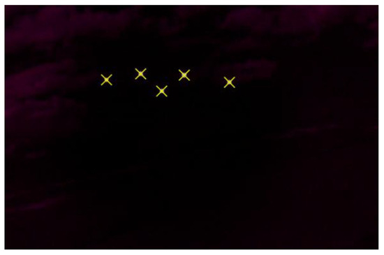
Figure 4.
Detection of the IR led markers in the fighter from a remote carrier.
This is in the fighter’s body frame but in a plane that is parallel to the navigation frame, i.e., only corrected by . It is important that this configuration is in the body frame rather than inertial frame to ensure that the leader is within the remote carrier’s camera field, in case it is used. It is also important to note that the inertial heading often differs from by a crab angle β as a result of wind. When traveling at the same velocity, in equivalent wind, β will be the same for both aircrafts. To account for this, is placed in the fighter’s inertial frame to form , where in Figure 4.
Firstly, position and velocity setpoints are calculated based on the relative position wanted in the formation flight; Figure 5 and Figure 6 describes the geometric relationship between the leader and setpoint state. Here, the leader is in a banked turn with heading rate which must be accounted for. Equations (48)–(50) calculate the geometric relationship.
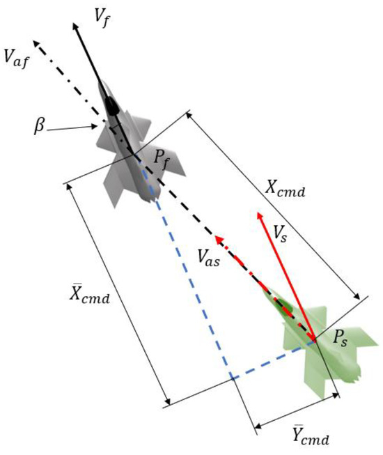
Figure 5.
Commanded relative position augmentation to compensate for the fighter crab angle.
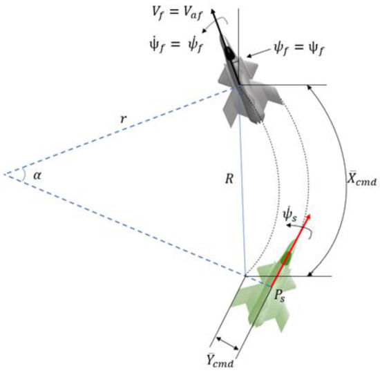
Figure 6.
Setpoint state during banked turn with lateral position offset command.
The setpoint position is then calculated in Equation (50), where and are rotation matrices around the z axis, as defined in Equation (51).
The setpoint velocity is then calculated in Equation (53).
where r is the radio of gyration and is
Finally, to converge to and track the setpoint, the error state is translated, in terms of the estimated relative state, to mid-level commands that our platform autopilot can accept. In our case, this is , and . To accomplish this, three control laws for positioning, velocities, and lateral acceleration have been developed. First, the position error calculation follows Equation (55).
where the commanded velocity is using horizontal and vertical gains and , respectively. The operator denotes element-wise multiplication.
In the case of velocity error, the longitudinal component is placed in the fighter wind frame, using the fighter airspeed .
For the lateral command, in Figure 7, which is the most complex dynamic in the close-formation flight, the lateral guidance aims to minimize the angle between the X-Y component of the desired air-relative velocity vector and the vehicle’s current air-relative velocity vector .
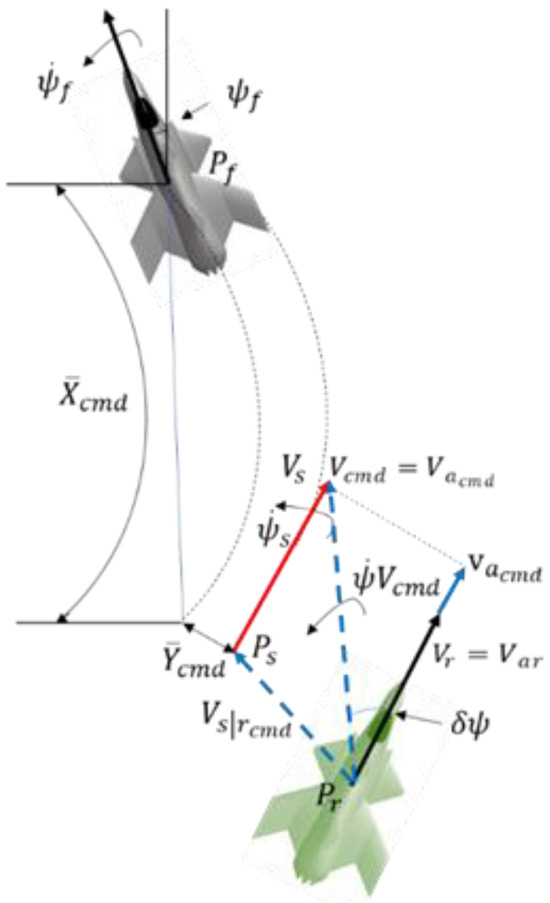
Figure 7.
A 2D depiction of vector guidance being used to transition to and maintain a commanded formation configuration.
First, the rotation rate of is calculated in Equation (61).
Then, the commanded rate is calculated using a lateral gain in Equation (62).
The bank angle command is then calculated using the commanded heading rate, follower airspeed and gravity g.
Position Setpoint Calculations
The MUM-T planner aerial module generates coordinated 3D formations of UAVs around a reference point, typically associated with a manned aircraft or a shared operational target. This planner supports a variety of tactical geometric arrangements—including Arrow, Line, cross, sphere, Plus, and Z formations—based on defined mission parameters, as show in Table 2 and Figure 8.
Table 2.
Formation types.
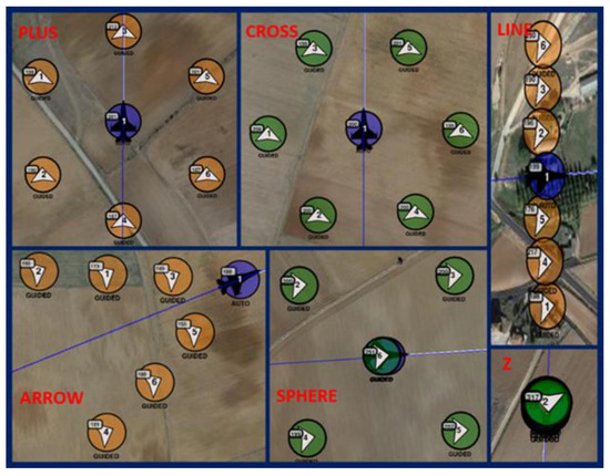
Figure 8.
Formations.
This functionality is designed specifically for Manned–Unmanned Teaming (MUM-T) contexts, where UAVs must assume predictable, geometrically controlled positions around a common reference to ensure coordination, deconfliction, and rapid deployment upon tasking.
These position setpoints will be the input of the relative navigation system.
The MUM-T planner parameters that can be defined are in the following Table 3.
Table 3.
Formation parameters.
The qualitative distance categories used in Table 3 are defined as follows:
- FAR: separation greater than 50 m;
- MEDIUM: between 35 and 50 m;
- NEAR: less than 10 m.
In multi-UAV mission scenarios involving Manned–Unmanned Teaming (MUM-T), the precise positioning of unmanned aerial vehicles relative to a central reference—typically a manned fighter aircraft—is critical to ensuring operational coherence, spatial deconfliction, and synchronized action. This section presents the mathematical formulation used to compute the relative coordinates of each UAV within a predefined formation geometry.
The UAVs are positioned with respect to a reference point (usually the first waypoint), which represents the center of the formation. The geometric layout is governed by the mission’s orientation heading, the selected formation type, and a lateral separation parameter defined by one of three possible standoff categories: FAR, MEDIUM, or NEAR. Altitude variation may also be introduced to establish a three-dimensional distribution depending on the formation configuration.
For each formation type, a specific rule is applied to compute the relative positions (, , ) of the UAVs in a local UTM coordinate frame. The following subsections define the equations used for calculating these positions. We begin with the Arrow formation, which creates a symmetric V-shape centered on the heading axis of the reference aircraft.
- Reference Point and Geometry
- The initial target point (first waypoint) is used as the center of the formation, where the fighter is.
- The altitude of each UAV may vary based on formation type and position.
- The formation orientation is derived from the following:
- ■
- Heading;
- ■
- Separation distance (FAR, MEDIUM, or NEAR).
- Position Assignment
For each position assignment corresponding to the formation types defined previously, the following sections detail how the target coordinates are computed for each UAV within the formation. These coordinates are defined relative to the leader’s frame and account for the spacing and topology constraints of the specific formation pattern.
- (a)
- Arrow
- UAVs placed in staggered angles along two arms diverging from the central axis.
- Uses a trigonometric offset with atan(2) for angular divergence.
The calculation of the relative waypoint is performed in the following way:For UAV i ∈ {0,…, N − 1}:- If i = 0: UAV at the center:
- If i > 0: UAVs placed in alternating directions:
- (b)
- Line
- UAVs distributed symmetrically along a line perpendicular to the heading.
- Alternates between left and right sides relative to the central axis.
Let heading angle α be in radians:For UAV i ∈ {0,…, N − 1}: - (c)
- Cross/Plus
- UAVs placed in four cardinal directions (0°, 90°, 180°, 270°) or full 360°.
- Uniform angular spacing computed from total UAV count.
For UAV i ∈ {0,…, N − 1}:Then - (d)
- Z
- UAVs stacked at increasing/decreasing altitudes with alternating lateral displacement.
For UAV i ∈ {0,…, N − 1}: - (e)
- Sphere
- One UAV positioned above and optionally one below the center.
- The rest are evenly distributed around a horizontal circumference.
Let
The rest are placed on a horizontal circle as in Plus formation.
For
- UAV 0 → directly above center:
- UAV 1 (if N even) → directly below:
- Remaining UAVs i ≥ 2 placed on the circle:
Let M = N − (number of vertical UAVs), then
where V = number of vertical UAVs (1 or 2)
- 3.
- Position Assignment
Each position is computed in UTM space and then converted back to geodetic coordinates.
4. Simulations
This section describes the high-fidelity simulation environment developed to evaluate the performance of the relative state estimator, the vision-based error management subsystem, and the mathematical consistency of the control and estimation architecture within a Manned–Unmanned Teaming (MUM-T) framework. The primary purpose of this simulator is not to emulate a complete formation flight mission, but rather to validate the correctness and robustness of the estimation pipeline under realistic sensor and communication conditions prior to hardware-in-the-loop or flight testing.
The simulation framework, Figure 9 and Figure 10, has been implemented using MATLAB Simulink 2019a, with the Aerospace Blockset and Aerosim Blockset providing a modular foundation for modeling the aircraft dynamics, actuator responses, and sensor suites. The UAVs and the manned fighter are modeled as nonlinear 6-degrees-of-freedom (6-DOF) systems, with actuators modeled via first-order lags, saturation limits, and rate constraints.
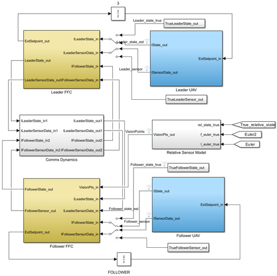
Figure 9.
Simulation environment.
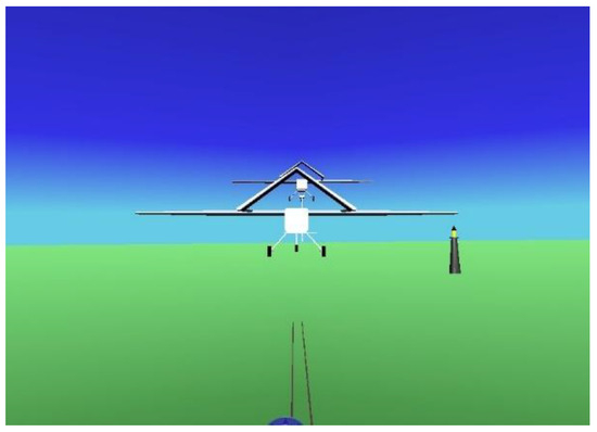
Figure 10.
Visualization in Matlab.
To create a representative environment, the simulation includes
- A gravity model,
- A geomagnetic field model,
- Atmospheric pressure and wind disturbances,
- Sensor models that incorporate bias, Gaussian white noise, and cross-axis coupling,
- GPS with Gauss–Markov drift,
- And crucially, communication latency and packet loss, especially affecting telemetry between the fighter and the remote carriers.
- The vision subsystem is modeled as a standard RGB camera with the following:
- Resolution: 1920 × 1080 pixels;
- Field of view (FOV): 70° horizontal × 42° vertical;
- Frame rate: 30 fps.
Fiducial markers are projected into image coordinates based on the relative position and orientation between the aircraft, using Equations (19) and (20). To reflect realistic limitations, the pixel stream is corrupted with white noise and randomized distortions, emulating occlusion, marker jitter, and partial dropout effects.
This controlled vision degradation is critical for validating the vision fault management strategy, which dynamically adjusts estimator confidence and fallback logic when visual information becomes unreliable or inconsistent.
- (a)
- Simulated UAV Models
The simulation includes a fleet of three fixed-wing VTOL UAVs, each defined by the following:
- Wingspan: 2500 mm
- Length: 1260 mm
- Material: Carbon fiber
- Empty weight (without battery): 7.0 kg
- Maximum Take-off Weight (MTOW): 15.0 kg
- Cruise speed: 26 m/s (at 12.5 kg)
- Stall speed: 15.5 m/s (at 12.5 kg)
- Max flight altitude: 4800 m
- Wind resistance:
- Fixed-wing: 10.8–13.8 m/s
- VTOL: 5.5–7.9 m/s
- Voltage: 12S LiPo
- Operating temperature: −20 °C to 45 °C
These characteristics ensure that the simulated agents reflect realistic operational constraints for medium-sized UAVs in tactical environments.
- (b)
- Simulation environment
All simulations were executed on a Lenovo Legion 5 16IRX8 laptop, equipped with
- CPU: Intel Core i7-13700HX
- Memory: 32 GB DDR5 RAM
- GPU: NVIDIA GeForce RTX 4070 (8 GB)
This setup enables real-time multi-agent simulation with sufficient fidelity for estimator tuning and controller evaluation.
As mentioned, the vision sensor was simulated as a normal camera, with a resolution of 1920 × 1080 pixels, a field of view of 70° × 42°, and a frame rate of 30 fps. A frame rate of 30 FPS was chosen as a trade-off between computational load and sufficient temporal resolution for close-range visual tracking. For the short-range relative estimation task, this rate proved adequate to maintain accurate marker detection and smooth estimation. Nonetheless, higher FPS (e.g., 60 or 90 FPS) would reduce latency and potentially improve robustness during fast maneuvers and will be considered in future implementations.
The field of view (FOV) is a crucial factor to consider when choosing a camera. It is essential to monitor all the markers during the close-formation flight procedure. In order to calculate the relative posture, it is necessary to simulate pixel coordinates. These coordinates are determined using Equations (18)–(20), taking into account the positions and attitudes of both the fighter and the remote carriers, as seen in Figure 7. Subsequently, white noise and a random arrangement were introduced into the pixel stream to replicate the simulated observations.
Figure 11 and Figure 12 depict the comparative orientation and location of the fighter and remote carrier, respectively. The green line represents the accurate data collected from the simulator, the red line represents the unprocessed data from each UAV, the intense blue line represents the vision measurements, and the light blue line represents the estimated data of the relative attitude and the position between UAVs.
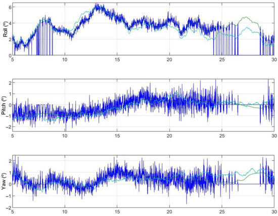
Figure 11.
Relative attitude.
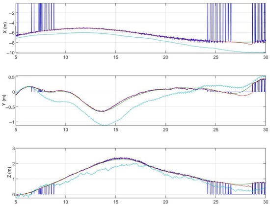
Figure 12.
Relative position.
Simulations had instances of vision dropouts, which are evident when the POSIT measurement reaches zero. The presence of vertical lines that reach zero denotes the start and end of the dropout. The vision problems can be ascribed to the markers located outside the field of view of the remote carrier. Despite significant setbacks in foresight, the estimator’s accuracy remains largely unaffected. Figure 13 shows relative velocities between aircraft. The intense blue is the true data obtained from the simulator, the red one is the raw data, and the green one is the estimator data, showing adequate robustness for the entrusted mission.
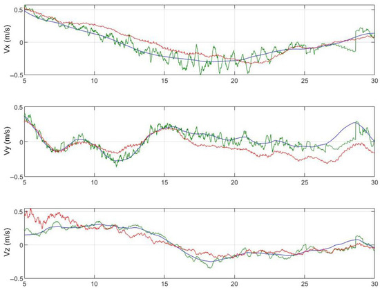
Figure 13.
Relative velocities.
Analysis
This section presents a quantitative evaluation of the accuracy of the relative state estimation subsystem used during formation flight experiments. The evaluation is based on a comparison between the estimated states and ground-truth references. Three key components are evaluated: relative position, relative velocity, and relative attitude. The comparison is expressed in terms of Mean Absolute Error (MAE) and Root Mean Square Error (RMSE), which are widely used metrics in estimation theory and control validation.
- Mean Absolute Error (MAE) quantifies the average magnitude of the estimation error. It provides a clear sense of the overall deviation between estimated and true values, regardless of the direction of the error. It is less sensitive to outliers and is often used to assess the average expected deviation in real applications.where is the estimated value at time step i, is the corresponding ground-truth value, and N is the total number of samples.
- Root Mean Square Error (RMSE) penalizes larger deviations more strongly due to the squaring of errors before averaging. RMSE is more sensitive to occasional large errors (outliers) and thus provides a better sense of estimation robustness and worst-case deviations. It is particularly relevant in systems where sporadic large errors may compromise performance or safety.where is the estimated value at time step i, is the corresponding ground-truth value, and N is the total number of samples.
While both metrics provide a measure of estimation accuracy, RMSE is more sensitive to large errors due to the squaring operation and is therefore more appropriate for detecting outliers or transient performance degradation. MAE, being less affected by extreme values, offers a more general sense of the overall estimation quality.
- Relative Position Estimation
Figure 14 illustrates the errors between the estimated relative position and the ground-truth relative position over time. The figure provides a visual representation of the estimation accuracy across the three spatial axes and highlights both the Mean Absolute Error (MAE) and the Root Mean Square Error (RMSE) values for each component. This visualization complements the quantitative analysis by showing not only the average performance but also the temporal dynamics and possible transient deviations of the estimation algorithm.
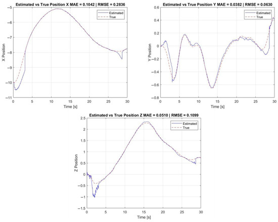
Figure 14.
Estimated vs. true position.
Table 4 summarizes the MAE and RMSE values between the estimated and true relative positions in the X, Y, and Z directions. In this configuration, the position estimation is primarily based on onboard inertial sensors and kinematic models, with vision-based measurements used as a secondary aiding source when available to improve drift correction and reduce long-term bias.
Table 4.
Relative position estimation of MAE and RMSE.
The lateral and vertical position estimates exhibit low error levels (MAE < 5 cm and RMSE < 11 cm). The longitudinal (X) component presents a higher RMSE of 28 cm, despite a moderate MAE of 10 cm. This discrepancy is explained by occasional discontinuities caused by a temporary loss or reacquisition of visual markers, which degrade the aiding signal provided by the vision system. These transient errors are better captured by the RMSE metric due to their sensitivity to outliers.
- 2.
- Relative Velocity Estimation
Figure 15 illustrates the errors between the estimated relative velocity and the ground-truth relative velocity over time. The plot presents the temporal evolution of the estimation error along each axis and includes the corresponding Mean Absolute Error (MAE) and Root Mean Square Error (RMSE) values. This figure provides insight into the dynamic behavior and precision of the velocity estimation algorithm, which relies solely on inertial measurements and onboard models.
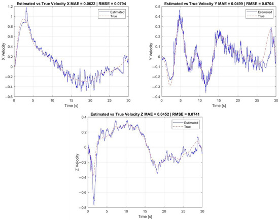
Figure 15.
Estimated vs. true velocity.
The relative velocity estimation is computed entirely from inertial measurements and onboard kinematic models and does not rely on any visual data. Table 5 provides the error metrics for the estimation of relative velocity.
Table 5.
Relative velocity estimation of MAE and RMSE.
The velocity estimation system shows uniformly low errors across all axes, with MAEs below 6.3 cm/s. The small differences between MAE and RMSE values indicate a consistent estimation performance with limited influence from transient deviations. These results confirm the robustness of the inertial-based estimation approach, particularly useful in environments with poor visual feedback or during visual marker occlusions.
- 3.
- Relative Attitude Estimation
Figure 16 illustrates the errors between the estimated relative attitude (roll, pitch, and yaw) and the corresponding ground-truth values over time. The figure includes the evolution of estimation errors for each rotational axis, along with the associated Mean Absolute Error (MAE) and Root Mean Square Error (RMSE) values. This visualization highlights the performance of the attitude estimation subsystem, which is primarily inertial-based and supported by visual corrections when available, and reveals the impact of transient discrepancies due to temporary visual marker loss or reacquisition.
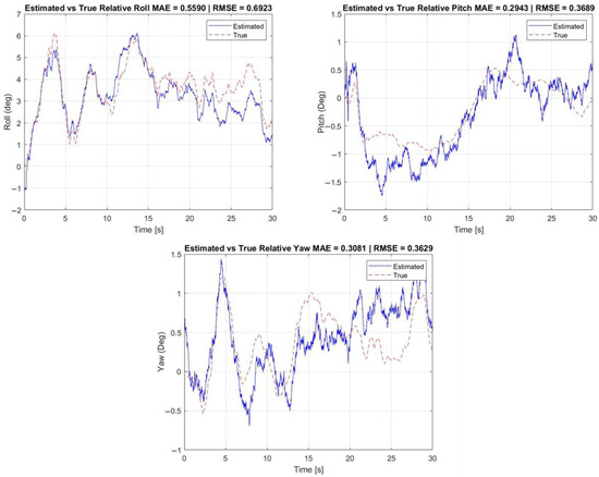
Figure 16.
Estimated vs. true attitude.
Table 6 provides the error metrics for the estimation of relative attitude angles. The attitude estimation algorithm is primarily driven by gyroscopic and inertial data, with vision-based pose information used as a complementary correction input when available.
Table 6.
Relative attitude estimation of MAE and RMSE.
All three attitude components demonstrate errors well below 1°, indicating high-quality orientation estimation. The pitch and yaw estimates are slightly more accurate than roll, which is more susceptible to cross-axis coupling and vision-related noise. Similarly to the position estimation case, outliers observed in the roll axis are likely caused by temporary disruptions in visual marker tracking, which affect the vision-aided correction process.
The combined analysis demonstrates that the relative estimation framework provides accurate and reliable outputs across all six degrees of freedom and their derivatives. The core estimation algorithms are inertial-driven, with visual data acting as an aiding mechanism that enhances long-term consistency. This design provides robustness against the temporary loss of visual information, while still benefiting from visual corrections when available. The low MAE and RMSE values across position, velocity, and attitude confirm that the system is well-suited for autonomous formation flight and cooperative navigation tasks in uncertain or visually degraded environments.
5. Experiments
For the experiments conducted in this paper, we utilized a swarming framework developed in the Robotic Operating System (ROS) and C++. This framework, independent of this study, enables the coordination of diverse robotic systems, including terrestrial, aerial, and aquatic platforms. Its modular architecture allows the seamless integration of new platforms and payloads, while C++ ensures high performance and real-time communication. The framework also interfaces with ArduPilot, providing a unified control interface for autonomous vehicles. This implementation facilitates efficient swarm coordination, making it a valuable tool for autonomous systems research.
The primary purpose of the Manned–Unmanned Teaming Air mission is to safeguard a fixed-wing vehicle, typically operated by a human pilot. A fleet of 2 remote carrier vehicles will trail after the UAV, simulating to be the fighter, maintaining a consistent formation around it. The level of protection will be contingent upon the following parameters:
- The selected vehicles will be evenly spaced around the leading vehicle, with the number of selected vehicles being taken into account.
- Placement: Depending on the selected formation, the vehicles will be positioned in different locations.
- ○
- In a PLUS (+) formation, the vehicles will be evenly dispersed around the leading vehicle, with one remote carrier positioned directly in front.
- ○
- The CROSS configuration (X) involves the equitable distribution of remote carriers surrounding the leading vehicle, with two vehicles positioned in front.
- ○
- ARROW formation: they will be positioned so that the tip of the arrow is the vehicle to follow.
- ○
- SPHERE formation: it is equivalent to CROSS formation, but one vehicle will be placed above and another below
- ○
- LINE formation: they will be distributed forming a line to the sides of the leader.
- ○
- Z formation: they will be distributed forming a vertical line above and below the leader.
The pilot has the authority to determine the distance between assets, with three separation options available: close, middle, or far, based on the desired proximity to the leader.
The MUM-T Human Machine Interface (HMI) will provide a live representation of the spatial configuration of each element in the MUM-T formation. The marked trajectories will enable operators to visually perceive the relative position between the manned aircraft and UAVs, both predicted and current. Furthermore, a dynamic depiction of restricted airspace will be included, computed according to the fighter’s dynamics and its anticipated future placements. The exclusion zones will undergo regular updates to guarantee both safety and efficiency in operations.
The determination of security levels between UAVs and manned aircraft will be based on their proximity and relative position and indicated with a color code, green, yellow, and red, based on the level of risk. The interface will offer both visual and aural alerts to notify operators of potential hazards, allowing them to make well-informed decisions to prevent dangerous situations. To ensure the safety of the manned aircraft and maintain the integrity of the MUM-T formation, we will employ collision detection and proximity detection algorithms, as shown in Figure 17.
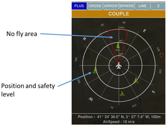
Figure 17.
MUM-T HMI.
The system will enable the control of various formations, adjusting to the individual requirements of the task. Operators have the ability to arrange formations in various tactical configurations such as line, wedge, square, or other arrangements depending on the mission objectives and environmental conditions. The interface will additionally enable the synchronization between UAVs and manned aircraft, enabling flexible adjustments in the arrangement to promptly react to unforeseen circumstances, as can be seen in Figure 17 and images below.
A prerequisite for initiating a MUM-T Air mission is the presence of a piloted vehicle within the swarm system. After being chosen, the vehicles can be directed to follow the selected target based on the specified characteristics. The MUM-T class constructor will handle declaring the ROS objects (subscribers, publishers, and services), as well as initializing variables or retrieving their values from the database. Following these fundamental initializations, you will acquire the precise location of the foremost car in order to determine the allocation of the other vehicles based on it. After the distribution is computed, each vehicle will commence moving towards its designated location.
After the mission is properly established, the commands sent to the autopilot will be adjusted whenever the leader’s position is updated. Furthermore, you will need to inquire about the velocities of the object, encompassing both its linear and angular motion.
Given that this mission lacks a predetermined sequence of waypoints and the movement of the vehicle to be tracked is not established, three distinct setpoints will be sent. These setpoints include the desired speed of the system, the desired bank angle, and the desired altitude above the ground. In order for the autopilot to process these commands, it is imperative that its operating mode is set to stabilize, which is used to control the UAV in attitude angles.
Once the system is in guided mode and receives the required data from the vehicle to be followed, it will calculate the setpoints to be delivered to the autopilot. The system will then wait for an output that aligns with the input parameters of the mission.
To ensure non-air collisions, there exists a collision detection module, which alters the flight altitude of each aircraft, and the height setpoint will cease to change in the mission whenever a potential collision is detected. This adjustment will consider the altitude commanded by the anti-collision module. This flowchart is explained in Figure 18.
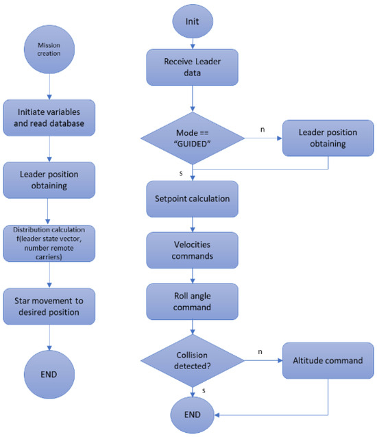
Figure 18.
MUM-T mission creation and execution.
This experiment involved the use of three unmanned aerial vehicles (UAVs) to test formation flying and mission re-tasking capabilities in a controlled environment. Two of the UAVs were configured to act as remote carriers (RCs), while the third simulated a fighter. The primary objectives were to analyze the ability of the group to fly in various geometric formations, perform a mission assigned to the remote carriers, and subsequently regroup with the fighter.
- Initial Configuration, Figure 19.
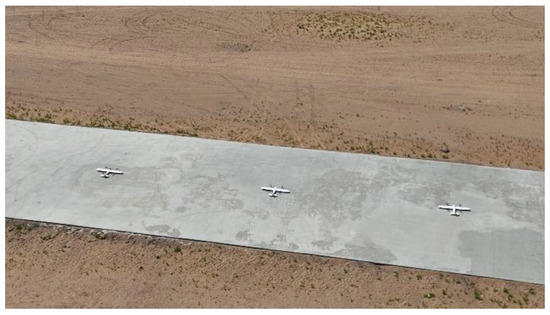 Figure 19. Test planes over the runway.
- ○
- Fighter UAV: Responsible for leading the formation and coordinating operations. This UAV acted as the central node for mission management.
- ○
- Remote Carriers: Equipped with limited autonomy capabilities, the two UAVs supported the fighter by executing specific tasks and following instructions.
- Parameters of the experiment:
Swarm Composition:
- Three fixed-wing VTOL UAVs:
- ○
- Wingspan: 2500 mm
- ○
- Length: 1260 mm
- ○
- Material: Carbon fiber
- ○
- Empty weight (no battery): 7.0 kg
- ○
- Maximum take-off weight: 15.0 kg
- ○
- Cruise speed: 26 m/s at12.5 kg
- ○
- Stall speed: 15.5 m/s at 12.5 kg
- ○
- Maximum flight altitude: 4800 m
- ○
- Wind resistance:
- ▪
- Fixed-wing mode: 10.8–13.8 m/s
- ▪
- VTOL mode: 5.5–7.9 m/s
- ○
- Operating voltage: 12S
- ○
- Temperature range: −20 °C to 45 °C
GCS:
- Executed on a Lenovo Legion 5 16IRX8 laptop:
- ○
- Intel Core i7-13700HX
- ○
- 32 GB DDR5 RAM
- ○
- NVIDIA GeForce RTX 4070 (8 GB)
- Communications:
- ▪
- XTEND 900MHz 1W for mesh communications
- ○
- Antenna omni 5 Dbi for airplane
Antenna omni 11 Dbi for ground
The methodology followed during the experiments is divided into different steps.
- Formation Flying: Several formation patterns were mentioned before for the UAVs, Figure 20, to adopt and maintain during flight. The experiment evaluated the stability and accuracy of each formation under varying flight conditions, including changes in speed, sharp turns, and turbulence (Figure 21).
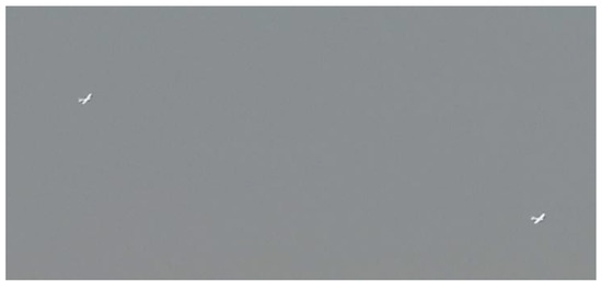 Figure 20. Two UAVs in formation flight.
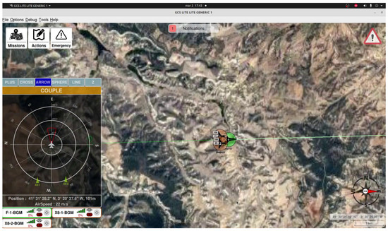 Figure 21. GCS view of the formation flight.
 - Mission Re-tasking: During the flight, the remote carriers were assigned a new mission that required them to temporarily leave the formation. The mission involved tasks such as simulating reconnaissance over a designated area (Figure 22).
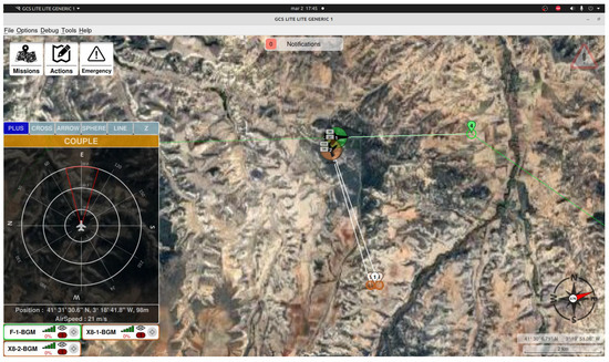 Figure 22. Two remote carrier re-tasking.
 - Regrouping: After completing their mission, the remote carriers returned to the main formation. The regrouping process followed a safe approach protocol to minimize interference and ensure a smooth return to their assigned positions within the formation (Figure 23).
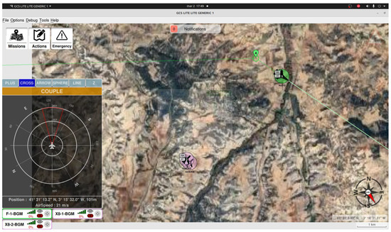 Figure 23. Two remote carriers rejoining.
The following results and observations were obtained during the test, Figure 24.
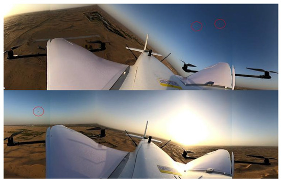
Figure 24.
Air to air view of the formation flight.
- Formation Stability: The formations were stable in simpler configurations, such as the Plus pattern. However, in more dynamic configurations like the Arrow formation, greater deviations were observed in the relative positions due to sensor navigation limitations.
- Re-Tasking Efficiency: The remote carriers successfully completed their assigned mission within an acceptable timeframe, although synchronization during regrouping with the fighter experienced minor delays in scenarios with increased simulated traffic density.
- Regrouping Success: Regrouping was successfully achieved in most trials, highlighting the importance of trajectory optimization algorithms in multi-UAV scenarios.
The following Figure 25 and Figure 26 show the different trajectories of the fighter and the remote carriers during various formation types, including Arrow, Line, and Z formations. It also illustrates the re-tasking of the two remote carriers as they temporarily leave the formation to execute a mission, followed by their subsequent regrouping with the fighter.
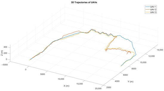
Figure 25.
Trajectories during the flight.
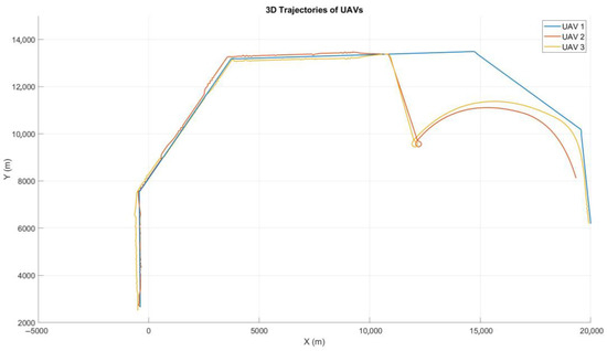
Figure 26.
Top view of the trajectories.
Analysis
To rigorously evaluate the safety and stability of the swarm’s decentralized collision avoidance mechanism, a detailed statistical analysis was conducted on inter-agent interactions throughout the flight. The methodology was applied pairwise to all UAVs in the swarm using synchronized trajectory data obtained from real flight experiments.
While the covariance matrices are not plotted for brevity, we observed consistent convergence behavior in the diagonal elements of the state covariance matrix across all estimation scenarios. The filter achieved steady-state values within the first 3–4 s of flight, indicating stable estimation performance.
First, inter-UAV distances were computed over time to classify proximity interactions into three severity levels:
- Risk: separation between 10 and 40 m.
- Danger: separation between 5 and 10 m.
- Near-collision: separation below 5 m.
Each category was quantified in terms of total event count, duration in seconds, and percentage of the total mission time. In parallel, Time to Collision (TTC) was calculated dynamically for each UAV pair based on their relative position and velocity vectors. TTC values provided insight into imminent threats not necessarily captured by spatial proximity alone.
A critical converging event was defined as a situation in which the following occurred:
- The UAVs had a relative heading <90°, indicating converging trajectories;
- The TTC was less than a defined threshold (5 s);
- The vertical separation was below 5 m.
These events were identified and visualized separately to highlight genuine risks of three-dimensional conflict, even in cases where horizontal separation appeared acceptable.
Beyond discrete event counting, several additional metrics were computed to support claims of overall system stability:
- Average separation distance between each UAV pair.
- Percentage of time with valid TTC, indicating the predictability of motion geometry.
- Rate of critical events per minute of flight, focusing exclusively on near-collisions and converging interactions.
All results were exported into a structured summary table (see Table 7) and supplemented with visual timelines and trajectory-based plots (see Figure 27 and Figure 28). This combination of geometric, kinematic, and statistical indicators provides a robust foundation for validating the swarm’s ability to maintain separation autonomously under dynamically evolving mission conditions.
Table 7.
Statistical analysis of risk events.
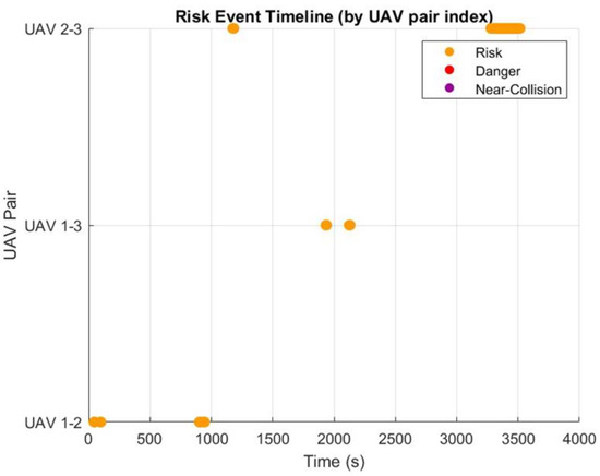
Figure 27.
Risk event timeline.
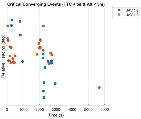
Figure 28.
Critical converging events.
Table 7 presents the results of a detailed pairwise analysis of UAV trajectories, focusing on proximity and heading convergence as indicators of potential collision risk. The dataset evaluates key metrics for three UAV pairs: UAV 1–2, UAV 1–3, and UAV 2–3. In all experiments, UAV 1 is designated as the leader, and the relative estimation is performed from the perspective of UAV 2 (wingman). The notation “UAV 1–2” therefore indicates an estimation of UAV 2’s state relative to UAV 1.
The following indicators were computed: minimum distance reached, number and duration of risk-related events, and percentage of mission time spent in each risk category. The categories include general Risk Events, Danger Events, Near-Collision Events, and Critical Converging Events (i.e., proximity events with heading alignment suggesting imminent convergence).
Pair UAV 1–2 reached a minimum separation of 34.77 m, triggering 61 risk events. These events accumulated a total of 30.17 s, corresponding to 0.51% of the total mission time. Additionally, 22 critical converging events were detected, with a cumulative duration of 10.88 s (0.18% of the mission time). No danger or near-collision events were recorded, indicating that although frequent, these interactions were not severe in nature.
Pair UAV 1–3 experienced slightly closer interactions, with a minimum distance of 29.35 m. A total of 30 risk events were logged, lasting 14.84 s (0.25% of the mission). Despite the reduced event count, the number of critical converging events was higher than in UAV 1–2 (23 events, lasting 11.38 s, or 0.19% of the mission), suggesting more alignment in velocity vectors during close encounters.
Pair UAV 2–3 showed the most concerning behavior, with the closest minimum distance of 19.67 m. This pair experienced a significantly higher number of risk events (474), totaling 234.47 s, which represents 3.98% of the mission time—an order of magnitude higher than the other pairs. However, only 18 of these events were classified as critically converging, indicating that while close-range operations were frequent, their converging nature was less prominent (0.15% of the time). Still, the elevated number and duration of risk events suggest a persistent violation of conservative safety margins.
Overall, while none of the pairs registered any Danger or Near-Collision events (0% in all cases), the high number of Risk and Critical Converging events—especially in the case of UAV 2–3—highlights the need for tuning inter-agent spacing policies and potentially modifying the collision avoidance or path planning strategies for improved long-term safety and stability of the swarm during operation.
6. Conclusions
This article introduced a vision-based state estimator for relative formation flight within a Manned–Unmanned Teaming (MUM-T) framework. The core of the system is an Unscented Kalman Filter (UKF), adapted to handle the nonlinearities of relative motion through the use of quaternions and Generalized Rodrigues Parameters (GRPs) for attitude error representation. This approach enables robust estimation during close-formation flight, even in the presence of sensor dropouts or poor initialization.
A high-fidelity simulation environment was developed to evaluate the estimator in a realistic 6-DOF nonlinear aircraft model. The UKF demonstrated strong performance in maintaining relative state accuracy under dynamic conditions and intermittent vision measurements. Experimental flight tests further validated the framework, confirming its applicability in real-world scenarios.
Key findings included the system’s ability to maintain stable formations in simple configurations, while more aggressive maneuvers revealed the need for refined controller tuning and better handling of navigation limitations. The framework also proved effective in managing dynamic mission re-tasking and regrouping, showcasing adaptability to evolving operational demands.
Future work will focus on integrating these findings into a more robust control and estimation architecture. Priorities include improved trajectory optimization for enhanced stability and adaptability, the mitigation of data latency and synchronization issues between platforms, and expanded testing under diverse environmental conditions, including GNSS-denied environments and higher wind variability. These efforts aim to ensure the reliability and operational readiness of the proposed system for broader deployment in manned–unmanned cooperative missions.
Author Contributions
Conceptualization, J.M.; Development, J.M.; Test, J.M.; Writing, J.M. and S.E. All authors have read and agreed to the published version of the manuscript.
Funding
This research received no external funding.
Data Availability Statement
Raw data supporting the tests and conclusions of this article will be made available by the authors under request.
Conflicts of Interest
The authors declare no conflicts of interest.
References
- Doebbler, J.; Spaeth, T.; Valasek, J.; Monda, M.J.; Schaub, H. Boom and receptacle autonomous air refueling using a visual pressure snake optical sensor. J. Guid. Control Dyn. 2007, 30, 1753–1769. [Google Scholar] [CrossRef]
- Johnson, E.N.; Watanabe, Y.; Ha, J.; Calise, A.J.; Tannenbaum, A.R. Image processing, estimation, guidance, and flight test of vision-based formation flight. In Proceedings of the 3rd International Symposium on Innovative Aerial/Space Flyer Systems, Tokyo, Japan, 24–25 November 2006. [Google Scholar]
- Khansari-Zadeh, S.M.; Saghafi, F. Vision-based navigation in autonomous close proximity operations using neural networks. IEEE Trans. Aerosp. Electron. Syst. 2011, 47, 864–883. [Google Scholar] [CrossRef]
- Mahboubi, Z.; Kolter, Z.; Wang, T.; Bower, G.; Ng, A.Y. Camera-based localization for autonomous UAV formation flight. In Proceedings of the AIAA Infotech Conference, St. Louis, MO, USA, 29–31 March 2011. [Google Scholar]
- Wilson, D.B.; Göktogan, A.H.; Sukkarieh, S. A vision based relative navigation framework for formation flight. In Proceedings of the IEEE International Conference on Robotics and Automation (ICRA), Hong Kong, China, 31 May–5 June 2014. [Google Scholar]
- Williamson, W.R.; Glenn, G.J.; Dang, V.T.; Speyer, J.L.; Stecko, S.M.; Takacs, J.M. Sensor fusion applied to autonomous aerial refueling. J. Guid. Control Dyn. 2009, 32, 262–275. [Google Scholar] [CrossRef]
- Hinchman, J.P.; Nalepka, J.L. Automated aerial refueling: Extending the effectiveness of unmanned air vehicles. In Proceedings of the AIAA Modeling and Simulation Technologies Conference and Exhibit, San Francisco, CA, USA, 15–18 August 2005. [Google Scholar]
- Lee, D.R.; Pernicka, H. Vision-based relative state estimation using the unscented kalman filter. Int. J. Aeronaut. Space Sci. 2011, 12, 24–36. [Google Scholar] [CrossRef]
- Oh, S.M.; Johnson, E. Relative motion estimation for vision-based formation flight using unscented kalman filter. In Proceedings of the AIAA Guidance, Navigation and Control Conference and Exhibit, Hilton Head, SC, USA, 20–23 August 2007. [Google Scholar]
- Kiim, S.; Kim, Y. Development of an MUM-T integrated simulation platform. IEEE Access 2023, 11, 21519–21533. [Google Scholar] [CrossRef]
- Heilemann, F.; Hollatz, F.; Schulte, A. Integration of mental resources in the planning of manned-unmanned teaming missions: Concept, implementation and evaluation. In Proceedings of the AIAA Scitech 2020 Forum, Orlando, FL, USA, 6–10 January 2020. [Google Scholar]
- Schmitt, F.; Brand, Y.; Rudnick, G.; Schulte, A. Experimental Evaluation of a Cooperative Automation Approach for Manned-Unmanned Teaming in Future Military Helicopter Missions; STO-MP-HFM-300; NATO: Brussels, Belgium, 2020; pp. 1–13. [Google Scholar]
- Ramírez-López, N.; Żbikowski, R. Effectiveness of Autonomous Decision Making for Unmanned Combat Aerial Vehicles in Dogfight Engagements. J. Guid. Control Dyn. 2018, 41, 1021–1024. [Google Scholar] [CrossRef]
- Huang, C.; Dong, K.; Huang, H.; Tang, S.; Zhang, Z. Autonomous air combat maneuver decision using Bayesian inference and moving horizon optimization. J. Syst. Eng. Electron. 2018, 29, 86–97. [Google Scholar] [CrossRef]
- Yang, J.-H.; Kapolka, M.; Chung, T.H. Autonomy balancing in a manned-unmanned teaming (MUT) swarm attack. In Robot Intelligence Technology and Applications 2012; Springer: Berlin/Heidelberg, Germany, 2013; Volume 208, pp. 561–569. [Google Scholar]
- Levulis, S.J.; DeLucia, P.R.; Kim, S.Y. Effects of Touch, Voice, and Multimodal Input, and Task Load on Multiple-UAV Monitoring Performance During Simulated Manned-Unmanned Teaming in a Military Helicopter. Proc. Hum. Factors Ergon. Soc. Annu. Meet. 2018, 60, 1117–1129. [Google Scholar] [CrossRef] [PubMed]
- Andrews, J.M. Human Performance Modeling: Analysis of the Effects of Manned-Unmanned Teaming on Pilot Workload and Mission Performance. Master’s Thesis, Defense Technical Informatiuon Center, Wright-Patterson Air Force Base, OH, USA, 2020. [Google Scholar]
- Julier, S.J.; Uhlmann, J.K.; Durrant-Whyte, H.F. A new approach for filtering nonlinear systems. In Proceedings of the 1995 American Control Conference-ACC’95, Seattle, WA, USA, 21–23 June 1995. [Google Scholar]
- Crassidis, J.L.; Markley, F.L. Unscented Filtering for Spacecraft Attitude Estimation. J. Guid. Control Dyn. 2003, 26, 536–542. [Google Scholar] [CrossRef]
- Dementhon, D.F.; Davis, L.S. Model-based object pose in 25 lines of code. Int. J. Comput. Vis. 1995, 15, 123–141. [Google Scholar] [CrossRef]
- Fosbury, A.; Crassidis, J. Relative navigation of air vehicles. J. Guid. Control Dyn. 2008, 31, 824–834. [Google Scholar] [CrossRef]
- Thomas, R.; van Riet, F.R. KC-10A refueling boom control system. In Proceedings of the IEEE National Aerospace and Electronics Conference (NAECON), Dayton, OH, USA, 20–22 May 1980. [Google Scholar]
- Smith, J.; Kunz, D. Simulation of the dynamically coupled KC-135 tanker and refueling boom. In Proceedings of the AIAA Modeling and Simulation Technologies Conference, Hilton Head, SC, USA, 20–23 August 2007. [Google Scholar]
- Mao, W.; Eke, F. A survey of the dynamics and control of aircraft during aerial refueling. Nonlinear Dyn. Syst. Theory 2008, 8, 375–388. [Google Scholar]
- Tharrett, D.L.; Pittaluga, A.E.; Decker, J.K.; Snelgrove, J.P. Robotic Autonomous Systems: Manned/Unmanned Teaming (RAS-MUM-T). Ph.D. Thesis, Naval Postgraduate School, Monterrey, CA, USA, 2020. [Google Scholar]
- Beni, G. Swarm Intelligence in Cellular Robotic Systems. In Robots and Biological Systems: Towards a New Bionics; NATO ASI Series; NATO: Brussels, Belgium, 1993; Volume 102, pp. 703–712. [Google Scholar]
- Beni, G. From Swarm Intelligence to Swarm Robotics. Swarm Robotics. In Lecture Notes in Computer Science; Springer: Berlin/Heidelberg, Germany, 2005; Volume 3342. [Google Scholar]
- Sahin, E. Swarm Robotics: From Sources of Inspiration to Domains of Application. In Proceedings of the 2004 International Conference on Swarm Robotics; Springer: Berlin/Heidelberg, Germany, 2005. [Google Scholar]
- Cao, Y.U.; Fukunaga, A.S.; Kahng, A. Cooperative Mobile Robotics: Antecedents and Directions. Auton. Robot. 1997, 4, 7–27. [Google Scholar] [CrossRef]
- Weiskopf, F.; Gion, T.; Elkiss, D.; Gilreath, H.; Bruzek, J.; Bamberger, R.; Grossman, K.; Wilkerson, J. Control of Cooperative, Autonomous Unmanned Aerial Vehicles. In Proceedings of the First AIAA Technical Conference and Workshop on UAV, Portsmouth, VA, USA, 20–23 May 2002. [Google Scholar]
- Dekker, A. A Taxonomy of Network Centric Warfare Architectures. Systems Engineering/Test and Evaluation. 2008, pp. 1–14. Available online: https://apps.dtic.mil/sti/citations/ADA488254 (accessed on 7 June 2025).
- Chung, T.H.; Jones, K.D.; Day, M.A.; Jones, M.; Clement, M. 50 vs. 50 by 2015: Swarm vs. Swarm UAV Live-Fly Competition at the Naval Postgraduate School. In Proceedings of the AUSVI Unmanned Systems, Washington, DC, USA, 12–15 August 2013; Volume 2, pp. 1792–1811. [Google Scholar]
- Parunak, H.V. Making Swarming Happen. In Proceedings of the Conference on Swarming and C4ISR, Tyson Corner, VA, USA, 3 January 2003. [Google Scholar]
- Frew, E.W.; Brown, T.X. Airborne Communication Networks for Small Unmanned Aircraft. Proc. IEEE 2009, 96, 2008–2027. [Google Scholar] [CrossRef]
- Kim, B.W.; Choi, G.E. Level and program analytics of MUM-T system. Int. J. Aeronaut. Space Sci. 2024, 25, 593–604. [Google Scholar] [CrossRef]
- Heilemann, F.; Schulte, A. Time line based tasking concept for MUM-T mission planning with multiple delegation levels. In Proceedings of the Advances in Intelligent Systems and Computing (AISC), Modena, Italy, 19–21 February 2020; Volume 1131. [Google Scholar]
- Taylor, G.; Turpin, T. Army aviation manned-unmanned teaming (MUM-T): Past, present, and future. In Proceedings of the 18th International Symposium on Aviation Psychology, Dayton, OH, USA, 4–7 May 2015. [Google Scholar]
- Mammarella, M.; Campa, G.; Napolitano, M.R.; Fravolini, M.L.; Gu, Y.; Perhinschi, M.G. Machine Vision/GPS Integration Using EKF for the UAV Aerial Refueling Problem. IEEE Trans. Syst. Man Cybern. Part C (Appl. Rev.) 2008, 38, 791–801. [Google Scholar] [CrossRef]
- Rogers, R.M. Applied Mathematics in Integrated Navigation Systems, 3rd ed.; AIAA Education Series; AIAA: Reston, VA, USA, 2007. [Google Scholar]
- Julier, S.J.; Uhlmann, J.K. A new extension of the Kalman filter to nonlinear systems. In Proceedings of the AeroSense: The 11th International Symposium on Aerospace/Defense Sensing, Simulation and Controls, Orlando, FL, USA, 21–23 April 1997. [Google Scholar]
- Rehbinder, H.X. Comparison of EKF and UKF for estimation of attitude and position of a rigid body. In Proceedings of the 2004 IEEE Conference on Decision and Control, Nassau, Bahamas, 14–17 December 2004; pp. 4729–4734. [Google Scholar]
- Van Der Merwe, R.; Wan, E.A.; Julier, S. Sigma-point Kalman filters for nonlinear estimation and sensor-fusion: Applications to integrated navigation. In Proceedings of the AIAA Guidance, Navigation and Control Conference and Exhibit, Rhode Island, RI, USA, 16–19 August 2004. [Google Scholar]
- Anderson, J.D. Introduction to Flight, 8th ed.; McGraw-Hill Education: New York, NY, USA, 2015. [Google Scholar]
- Weiss, S.; Achtelik, M.W.; Lynen, S.; Chli, M.; Siegwart, R. Real-time onboard vis-ual-inertial state estimation and self-calibration of MAVs in unknown environments. In Proceedings of the ICRA 2013, Karlsruhe, Germany, 6–10 May 2013; pp. 957–964. [Google Scholar]
Disclaimer/Publisher’s Note: The statements, opinions and data contained in all publications are solely those of the individual author(s) and contributor(s) and not of MDPI and/or the editor(s). MDPI and/or the editor(s) disclaim responsibility for any injury to people or property resulting from any ideas, methods, instructions or products referred to in the content. |
© 2025 by the authors. Licensee MDPI, Basel, Switzerland. This article is an open access article distributed under the terms and conditions of the Creative Commons Attribution (CC BY) license (https://creativecommons.org/licenses/by/4.0/).