Visual Active SLAM Method Considering Measurement and State Uncertainty for Space Exploration

Abstract

This paper presents a visual active SLAM method considering measurement and state uncertainty for space exploration in urban search and rescue environments. An uncertainty evaluation method based on the Fisher Information Matrix (FIM) is studied from the perspective of evaluating the localization uncertainty of SLAM systems. With the aid of the Fisher Information Matrix, the Cramér–Rao Lower Bound (CRLB) of the pose uncertainty in the stereo visual SLAM system is derived to describe the boundary of the pose uncertainty. Optimality criteria are introduced to quantitatively evaluate the localization uncertainty. The odometry information selection method and the local bundle adjustment information selection method based on Fisher Information are proposed to find out the measurements with low uncertainty for localization and mapping in the search and rescue process. By adopting the method above, the computing efficiency of the system is improved while the localization accuracy is equivalent to the classical ORB-SLAM2. Moreover, by the quantified uncertainty of local poses and map points, the generalized unary node and generalized unary edge are defined to improve the computational efficiency in computing local state uncertainty. In addition, an active loop closing planner considering local state uncertainty is proposed to make use of uncertainty in assisting the space exploration and decision-making of MAV, which is beneficial to the improvement of MAV localization performance in search and rescue environments. Simulations and field tests in different challenging scenarios are conducted to verify the effectiveness of the proposed method.

1. Introduction

In recent years, much attention has been paid to simultaneous localization and mapping (SLAM) and it has been applied in many different scenarios, such as indoor localization [1], search and rescue [2], inspection [3], autonomous driving [4,5], environment reconstruction [6], and underground exploration [7]. However, as the robot moves, the pose uncertainty increases. In terms of visual SLAM, the localization accuracy will decrease over time, especially when no loop is detected. Hence, for practical application considerations, it is necessary for a robot, such as UAV [8,9] or UGV [10,11], to find a collision-free trajectory that is beneficial both to decrease the uncertainty of pose estimation and to perform other tasks, such as coverage planning and exploration. This problem, which involves both SLAM and path planning, is known as active SLAM, and is considered to be one of the opening and challenging problems in mobile robotics.

In this work, we focus more on the uncertainty in visual active SLAM systems. A visual active SLAM method considering measurement and state uncertainty for space exploration is proposed. The novelty of the proposed method lies in that it realizes the quantification of both measurement and state uncertainty, and the quantification results are utilized in the design of perception-aware planning method. Compared with the existing results, the computational efficiency and MAV localization accuracy are improved through measurement and state uncertainty quantification while performing space exploration tasks with stereo camera in urban search and rescue environments.

The main contributions of this work are as follows:

• The perception-aware planning method makes full use of Fisher Information Matrix (FIM) and the uncertainty quantification metric for measurement information selection and path planning to improve MAV localization performance.
• The Cramér–Rao Lower Bound (CRLB) of the pose uncertainty in the stereo SLAM system is derived to describe the boundary of the pose uncertainty.
• The visual odometry information selection method and local bundle adjustment information selection method considering measurement uncertainty are proposed to improve the computational efficiency in both the front-end and back-end of the system.
• The generalized unary node and generalized unary edge are defined to quantify local state uncertainty and to improve the computational efficiency in computing local state uncertainty. Further, the perception-aware active loop closing planning method considering local state uncertainty is proposed for MAV space exploration and decision-making, which is beneficial to improving MAV localization performance.

The rest of this paper is structured as follows. Section 2 provides an overview of related work in active SLAM. Section 3 explains the uncertainty in visual SLAM and derives the CRLB of the pose uncertainty in stereo visual SLAM systems. In Section 4, we present the system overview and explain the proposed method in detail. Section 5 provides qualitative and quantitative results and analysis of the proposed method. Finally, we conclude the paper in Section 6.

2. Related Work

The conception of active SLAM was first proposed in [12]. It aims at integrating active perception into SLAM and can be defined as the problem of reducing the uncertainty of localization and map representation while performing SLAM [13,14].

To deal with the uncertainty of localization, different kinds of active SLAM approaches are proposed based on the uncertainty quantification [8,15,16,17,18,19,20]. In [15], the paramount importance of representing and quantifying uncertainty is highlighted to correctly report the associated confidence of the robot pose estimation. In [8], an active SLAM framework for mobile robots to find a collision-free trajectory with good performance in SLAM uncertainty reduction is presented. In [17], the Fisher Information Matrix and Cramér–Rao Lower Bound are derived based on the assumption of isotropic Langevin noise for rotation and block-isotropic Gaussian noise for translation and shown to be closely related to the graph structure of pose-graph SLAM. In [18], an application of Kullback–Leibler divergence is proposed for the purpose of evaluating the particle-based SLAM posterior approximation, which allows the robot to autonomously decide between exploration and place revisiting actions. In [19], the uncertainty evaluation is performed for the 3-D position estimation of each map point obtained from the depth measurement of the RGB-D camera. In [20], the selection of the visual cues is guided by the visual-inertial system performance quantification metric.

Moreover, to reduce the uncertainty of exploration and improve the accuracy of robot localization, many perception-aware planning methods have been proposed [21,22,23,24,25]. In [21], perception-aware planning methods for differentially flat robots are designed and discussed in detail. In [22], a topology-guided perception-aware receding horizon trajectory generation method is proposed to keep more visual features in view and improve localization accuracy. In [23], feature matchability is taken into account during trajectory planning. In [24], a perception-aware trajectory planning strategy for quadrotors is proposed to ensure the safety and localization accuracy. In [25], a perception-and-energy-aware motion planning method is presented to realize energy-efficient and reliable flight.

Inspired by [17,20], in this work, we derive the CRLB of the pose uncertainty in visual SLAM system with stereo camera. Differing from the previous work, in this work, we propose an information selection method considering measurement uncertainty to improve the efficiency of the algorithm. Further, we define the generalized unary node and generalized unary edge, and design a perception-aware active loop closing planner considering local state uncertainty to improve the localization accuracy when performing autonomous space exploration in search and rescue environments.

3. Uncertainty in Visual SLAM

In this paper, we followed the classical ORB-SLAM2 [26] algorithm framework, based on which, the algorithm is improved and optimized for the evaluation of pose uncertainty, which further facilitates the progress of MAV decision-making. Therefore, in this section, we focus on deriving the propagation and representation of uncertainty for SLAM systems using stereo camera based on graph optimization under this framework.

3.1. Graph Optimization Theory in Visual SLAM

The graph optimization theory-based SLAM method integrates graph theory with nonlinear optimization and adopts a graph representation to solve the estimation problem in SLAM, which mainly includes robot pose estimation and map point 3D position estimation. A graph consists of a number of nodes and edges that connect the nodes. Nodes are used to represent the states to be optimized and edges are used to represent measurement information or measurement error items. The process of generating constraints between nodes from the measured information is known as data association. A certain range of measurement constraints is usually selected to form a relatively simple topological complement structure so as to keep the complexity of data association as low as possible. In this work, the nodes are the MAV poses and the positions of the map points, while the edges are mainly the reprojection errors and the relative pose errors between image frames. Specifically, the following optimization processes are involved in the algorithm.

(1) Camera pose optimization for single image frames. The node is the camera pose corresponding to the current image frame, since only the pose is optimized and not the map points, and the edges are the unary edges composed of reprojection errors corresponding to a number of map points.

(2) Local Bundle Adjustment Optimization. The nodes are the camera pose corresponding to the current keyframe and the covisibility keyframe, the camera pose corresponding to the keyframe where the map points in the current keyframe and the covisibility keyframe are observed, and the map points in the current keyframe and the covisibility keyframes. The edges are the binary edges connecting the camera pose and the map points formed by the reprojection error of the above map points in the image frame in which the map points are observed.

(3) Global pose optimization. Nodes are the camera poses corresponding to all keyframes in the current map. The edges are binary edges composed of relative positional errors between camera poses.

(4) Local pose and map point optimization. Nodes are the position coordinates of camera poses and map points corresponding to all keyframes in the map. The edges are the binary edges consisting of the relative pose errors between the camera poses and the reprojection errors of the map points in the corresponding image frames.

In summary, in any case, once the SLAM problem is considered as graph optimization, the state to be optimized is associated with the observed information through data association. With the assumption that the measurement noise is Gaussian white noise, the final goal of the SLAM method based on graph optimization is to find the optimal estimate of the state to be optimized such that the posterior probability is maximized in that state.

Generally, the state to be optimized is denoted as x. In SLAM algorithms, the state estimation is to solve for the conditional probability distribution $P\left(x\right|z)$ of the state x under the condition that the measurement z is available. According to the definition of conditional probability and Bayesian law,

$$P\left(x\right|z)={\displaystyle \frac{P(x,z)}{P\left(z\right)}}={\displaystyle \frac{P\left(z\right|x\left)P\right(x)}{P\left(z\right)}}$$

(1)

We can find that the denominator of Equation (1) is independent of the state x. The posterior probability $P\left(x\right|z)$ of $P{\left(z\right)}^{-1}$ is the same for any state x. Thus, for the simplicity of formulation, $P{\left(z\right)}^{-1}$ can be expressed in terms of the normalized variable $\eta$. The above equation turns into

$$P\left(x\right|z)=\eta P(z\left|x\right)P\left(x\right)$$

(2)

In the equation above, $P\left(z\right|x)$ is the likelihood and $P\left(x\right)$ is the prior probability. Solving for x to maximize the posterior probability can be expressed as

$$x_{MAP}^{\ast }=argmaxP\left(z\right|x)P\left(x\right)$$

(3)

In an unknown environment with no prior information, the maximum likelihood estimate of x can be solved. The equation is as follows.

$$x_{MLE}^{\ast }=\arg \max P\left(z\right|x)$$

(4)

The maximum likelihood estimate in the above equation can be intuitively understood as the state under which the available measurements are most likely to be obtained. The maximum likelihood estimation can be solved by least squares. For the visual SLAM problem in this work, the poses of the camera are represented in the form of a Lie algebra. The optimization problem for the poses can be formulated as finding the optimal camera pose that minimizes the reprojection error, i.e.,

$${\xi }^{\ast }=\arg \underset{\xi }{\min }{\displaystyle \frac{1}{2}}\sum _{i=1}^n\rho {∥u_i-{\displaystyle \frac{1}{s_i}}Kexp\left({\xi }^{\wedge }\right)P_i∥}_2^2$$

(5)

In the above equation, $\xi$ is the Lie algebraic form of the camera pose. $u_i$ denotes the pixel coordinates of the i-$th$ spatial point in the image. $s_i$ denotes the scale. K denotes camera intrinsics. $P_i$ denotes 3D coordinates of spatial points. $\rho$ denotes robust kernel functions. Similarly, the optimization of the poses and map points optimization can be expressed as follows.

$${(\xi ,P)}^{\ast }=arg\underset{\xi ,P}{min}{\displaystyle \frac{1}{2}}\sum _{i=1}^m\sum _{j=1}^n\rho {∥u_j-{\displaystyle \frac{1}{s_j}}Kexp\left({\xi }_i^{\wedge }\right)P_j∥}_2^2$$

(6)

As mentioned above, the parameters and error items to be optimized in the least-squares expression of the SLAM problem correspond to the nodes and edges in the graph optimization. Considering the complex nonlinear relationship between the reprojection error of the pixel coordinates in the image and the camera pose and map points, the essence and core of the problem is a nonlinear least-squares problem. The relationship between reprojection and camera poses and map points will be described in detail in Section 3.3 during the derivation of the Cramér–Rao lower bound for the localization uncertainty.

3.2. Cramér–Rao Lower Bound and Fisher Information Matrix

Assuming that the probability density function $p(z;\theta )$ satisfies the regularity condition, where z denotes the measurement and $\theta$ denotes the estimated parameter, i.e., $\forall \theta$,

$$E\left[{\displaystyle \frac{\mathit{\partial }lnp(z;\theta )}{\mathit{\partial }\theta }}\right]=0$$

(7)

Then, the covariance for any unbiased estimation $\widehat{\theta }$ will always satisfy the following inequality.

$$Cov(\widehat{\theta })⪰I^{-1}\left(\theta \right)$$

(8)

$I^{-1}\left(\theta \right)$ in Equation (8) is Cramér–Rao Lower Bound, and it equals the inverse of the Fisher Information Matrix. The equation above indicates that $Cov(\widehat{\theta })-I^{-1}\left(\theta \right)$ is positive semi-definite, where $I\left(\theta \right)$ is the Fisher Information Matrix, defined as follows.

$$I\left(\theta \right)=-E\left[{\displaystyle \frac{{\mathit{\partial }}^{2}lnp(z;\theta )}{\mathit{\partial }{\theta }^2}}\right]$$

(9)

The lower bound determines the lower limit of the covariance of the unbiased estimation. In the case that the measurements are independent of each other and obey the same zero-mean Gaussian distribution $N\left(0,{\sigma }^2\right)$, the Fisher Information Matrix can be written in the following form.

$$I\left(\theta \right)=J^T\left(\theta \right){Cov}^{-1}\left(z\right)J\left(\theta \right)$$

(10)

In the above equation, $Cov\left(z\right)$ is the covariance matrix of the measurements and $J\left(\theta \right)$ is the Jacobian matrix consisting of the partial derivatives of the measurements with respect to the estimated parameters, i.e.,

$$J\left(\theta \right)={\displaystyle \frac{\mathit{\partial }z}{\mathit{\partial }\theta }}$$

(11)

Due to the assumption of independent identical distribution, Equation (10) can be further simplified as

$$I\left(\theta \right)={\displaystyle \frac{1}{{\sigma }^2}}{J}^T\left(\theta \right)J\left(\theta \right)$$

(12)

It is notable that the nonlinear maximum likelihood estimation is usually biased, but as the amount of Fisher Information increases, the bias also tends to decrease. Due to the rich theoretical implications of the Fisher Information Matrix, it is widely used in different applications, such as the Theory of Optimal Experimental Design (TOED) [27], Active SLAM [28], and information selection [20], etc. In [17], due to the different noise assumptions, the noise for the rotation part is different from the Gaussian noise, and Equation (12) may not be suitable. Thus, the rigorous CRLB is derived based on the assumption of zero-mean isotropic Langevin noise for orientation and block-isotropic Gaussian noise. In this work, we assume that the measurements (reprojection errors) are independent of each other and follow a Gaussian distribution, so that the Fisher Information Matrix takes the form of Equation (12). Given the variance of measurements, it is sufficient to calculate the Jacobian matrix of the reprojection error of pixel coordinates with respect to the poses and map points. The detailed derivation is presented in Section 3.3.

3.3. Cramér–Rao Lower Bound of Uncertainty for Visual SLAM with Stereo Camera

In the SLAM algorithm of this work, the uncertainty of the algorithm mainly lies in two aspects; one is the uncertainty of camera poses and the other is the uncertainty of map points. This section focuses on deriving the Jacobian matrix of the stereo visual SLAM reprojection error with respect to the poses and map points and then deriving the Cramér–Rao lower bound on the uncertainty of stereo visual SLAM with the help of the Fisher Information Matrix. The sensor mainly used in this system is a stereo camera.

Consider the coordinate of the spatial point in the world coordinate system as $P_w\left(X_w,Y_w,Z_w\right)$. Then, transform the point to the camera coordinate system with the coordinate $P_c\left(X_c,Y_c,Z_c\right)$. The following relationships can be derived from the camera projection model.

$$u=f_x{\displaystyle \frac{X_c}{Z_c}}+c_x$$

(13)

$$v=f_y{\displaystyle \frac{Y_c}{Z_c}}+c_y$$

(14)

$$u_r=f_x{\displaystyle \frac{X_c}{Z_c}}+c_x-{\displaystyle \frac{bf}{Z_c}}$$

(15)

In the equations above, u and v are the coordinates of the pixel points corresponding to the left camera. $u_r$ indicates the horizontal coordinate of the pixel point corresponding to the right camera. Denote the reprojection error of $\left(u,v,u_r\right)$ as e. Multiplying a perturbation $\delta \xi$ left for ${\xi }^{\wedge }$ and considering the partial derivative of the error with respect to the perturbation, using the chain law, we can obtain

$${\displaystyle \frac{\mathit{\partial }e}{\mathit{\partial }\delta \xi }}={\displaystyle \frac{\mathit{\partial }e}{\mathit{\partial }{P}_c}}{\displaystyle \frac{\mathit{\partial }{P}_c}{\mathit{\partial }\delta \xi }}=J\left(\xi \right)$$

(16)

The equation above is the Jacobian matrix for the pose optimization, where

$${\displaystyle \frac{\mathit{\partial }e}{\mathit{\partial }{P}_c}}=-\left[\begin{array}{ccc}{\displaystyle \frac{\mathit{\partial }u}{\mathit{\partial }{X}_c}}\hfill & {\displaystyle \frac{\mathit{\partial }u}{\mathit{\partial }{Y}_c}}\hfill & {\displaystyle \frac{\mathit{\partial }u}{\mathit{\partial }{Z}_c}}\hfill \\ {\displaystyle \frac{\mathit{\partial }v}{\mathit{\partial }{X}_c}}\hfill & {\displaystyle \frac{\mathit{\partial }v}{\mathit{\partial }{Y}_c}}\hfill & {\displaystyle \frac{\mathit{\partial }v}{\mathit{\partial }{Z}_c}}\hfill \\ {\displaystyle \frac{\mathit{\partial }{u}_r}{\mathit{\partial }{X}_c}}\hfill & {\displaystyle \frac{\mathit{\partial }{u}_r}{\mathit{\partial }{Y}_c}}\hfill & {\displaystyle \frac{\mathit{\partial }{u}_r}{\mathit{\partial }{Z}_c}}\hfill \end{array}\right]=-\left[\begin{array}{ccc}{\displaystyle \frac{f_x}{Z_c}}& 0& -{\displaystyle \frac{f_x{X}_c}{Z_c^2}}\\ 0& {\displaystyle \frac{f_y}{Z_c}}& -{\displaystyle \frac{f_y{Y}_c}{Z_c^2}}\\ {\displaystyle \frac{f_x}{Z_c}}& 0& -{\displaystyle \frac{f_x{X}_c-bf}{Z_c^2}}\end{array}\right]$$

(17)

$${\displaystyle \frac{\mathit{\partial }{P}_c}{\mathit{\partial }\delta \xi }}=\left[I_{3\times 3},-P_c^{\wedge }\right]$$

(18)

The projection model of $\left(u,v,u_r\right)$ in Equations (16)–(18) can be found in Equations (13)–(15), respectively.

To optimize the map points, the partial derivative of the error item with respect to the map points is calculated, i.e.,

$${\displaystyle \frac{\mathit{\partial }e}{\mathit{\partial }{P}_w}}={\displaystyle \frac{\mathit{\partial }e}{\mathit{\partial }{P}_c}}{\displaystyle \frac{\mathit{\partial }{P}_c}{\mathit{\partial }{P}_w}}=J\left(P_w\right)$$

(19)

The equation above is the Jacobian matrix for map point optimization, where

$${\displaystyle \frac{\mathit{\partial }{P}_c}{\mathit{\partial }{P}_w}}={\displaystyle \frac{\mathit{\partial }\left(R{P}_w+t\right)}{\mathit{\partial }{P}_w}}=R$$

(20)

At this point, two Jacobian matrices, which are extremely essential for the optimization of stereo visual SLAM poses and map points, are derived. Meanwhile, the above Jacobian matrix is crucial for the derivation of the Cramér–Rao Lower Bound on the uncertainty of stereo visual SLAM as well.

Let the covariance matrix of the pixel reprojection error be ${\Sigma }_{uvr}$. Then, the Fisher Information Matrix regarding the pose optimization is as follows.

$$I\left(\xi \right)=J^T\left(\xi \right){\Sigma }_{vvr}^{-1}J\left(\xi \right)$$

(21)

Similarly, Equation (22) denotes the Fisher Information Matrix regarding the map points optimization.

$$I\left(P_w\right)=J^T\left(P_w\right){\Sigma }_{wv}^{-1}J\left(P_w\right)$$

(22)

Under the definition of the Cramér–Rao Lower Bound, the Cramér–Rao Lower Bound for poses uncertainty is $I^{-1}\left(\xi \right)$, and the Cramér–Rao Lower Bound for map points uncertainty is $I^{-1}\left(P_w\right)$. By utilizing the relationship between the Cramér–Rao Lower Bound and the Fisher Information Matrix, the Fisher Information Matrix can be calculated based on the relationship between the measurement and the variable to be optimized during the SLAM uncertainty evaluation, and the uncertainty in the current state can be evaluated using appropriate metric criteria. Several optimality criteria are introduced in the next section.

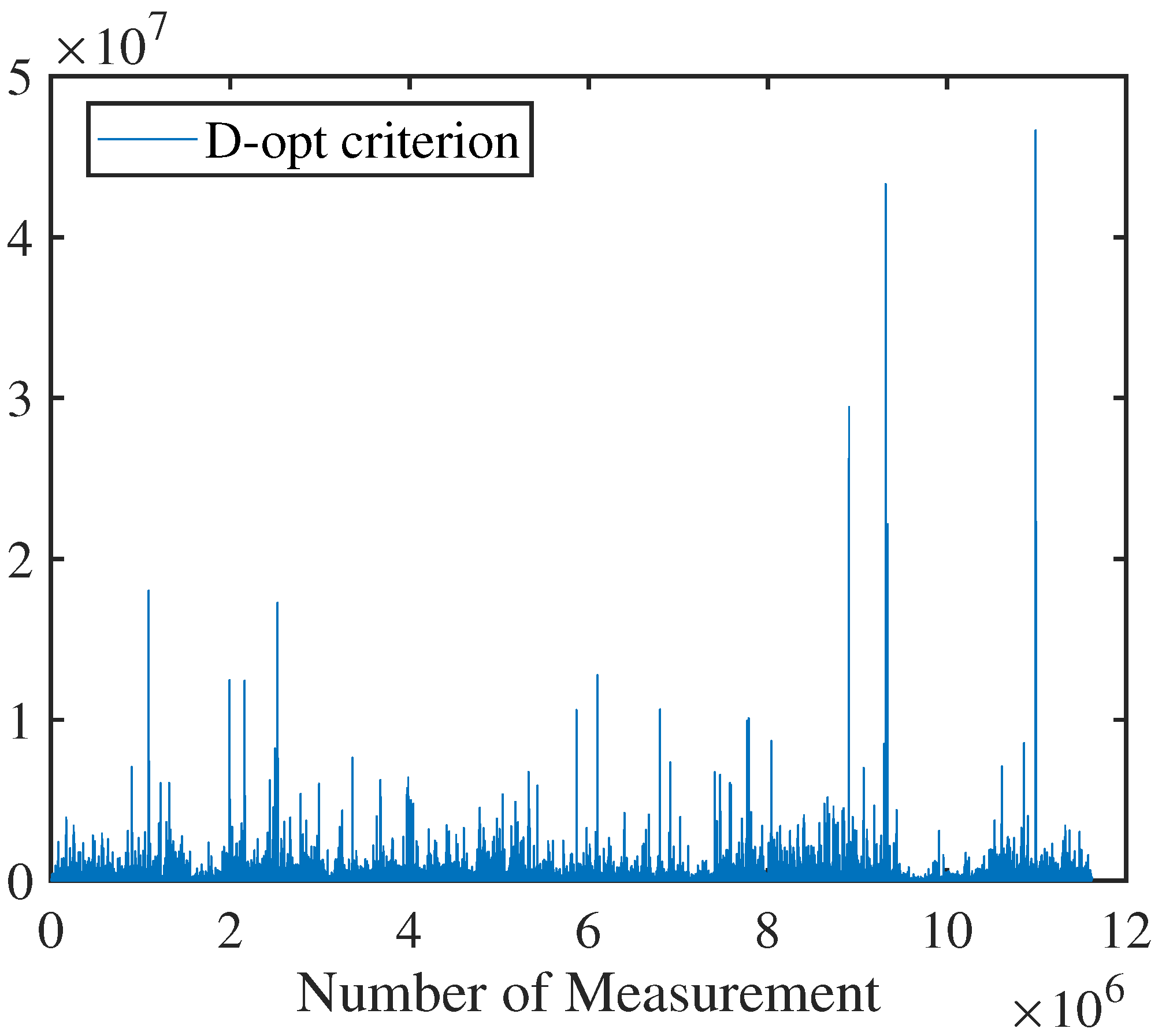
3.4. Optimality Criteria

In terms of quantifying uncertainty, Kiefer found, on the basis of TOED, that there exists a series of mappings [29], i.e.,

$${\parallel \Sigma \parallel }_p\to \mathbb{R}$$

(23)

The mapping depends mainly on the parameters p.

$${\parallel \Sigma \parallel }_p\triangleq {\left({\displaystyle \frac{1}{l}}trace\left({\Sigma }^p\right)\right)}^{{\displaystyle \frac{1}{p}}}$$

(24)

where l denotes the dimension of the state to be estimated and $\Sigma \in R^{l\times l}$ the covariance matrix that measures the uncertainty of the system, which is a symmetric positive semi-definite matrix. As mentioned before, the Cramér–Rao Lower Bound of this matrix is the inverse of the corresponding Fisher Information Matrix. In the quantitative analysis of uncertainty in this work, we focus on quantifying the Cramér–Rao Lower Bound of uncertainty.

Equation (24) can be transformed according to the value of p, as shown in the following equation.

$${\parallel \Sigma \parallel }_p=\left\{\begin{array}{cc}\sqrt[p]{{\displaystyle \frac{1}{l}}trace\left({\Sigma }^p\right)}& 0<\left|p\right|<\infty \\ det{(\Sigma )}^{{\displaystyle \frac{1}{l}}}& p=0\end{array}\right.$$

(25)

Using the matrix power property, the above equation can also be expressed as

$${\parallel \Sigma \parallel }_p=\left\{\begin{array}{cc}{\left({\displaystyle \frac{1}{l}}{\sum }_{k=1}^l{\lambda }_k^p\right)}^{{\displaystyle \frac{1}{p}}}& 0<\left|p\right|<\infty \\ exp\left({\displaystyle \frac{1}{l}}{\sum }_{k=1}^{l}log\left({\lambda }_k\right)\right)& p=0\end{array}\right.$$

(26)

where ${\lambda }_k$ is the eigenvalues of the matrix.

The above quantitative representation of uncertainty is essentially a function of the eigenvalues of the covariance matrix. From Equation (26), several commonly used optimality criteria for evaluating uncertainty can be deduced.

(1) T-opt criterion ($p=1$): Calculate the mean of the covariance, denoted by the trace of the normalized covariance matrix. The metric is easy to compute and the computational burden is small, but large eigenvalues may have a large impact on the whole metric, so it provides similar results to evaluating only the largest eigenvalues.

$$T-opt\triangleq {\displaystyle \frac{1}{l}}\sum _{k=1}^l{\lambda }_k$$

(27)

(2) A-opt criterion ($p=-1$): Calculate the summed mean of the covariance. The criterion is sensitive to outliers whose values are much smaller than the rest of the data, different from the T-opt criteria, which ignores these outliers, but the A-opt criterion is insensitive to extremely large outliers.

$$A-opt\triangleq {\left({\displaystyle \frac{1}{l}}\sum _{k=1}^l{\lambda }_k^{-1}\right)}^{-1}$$

(28)

(3) D-opt criterion ($p=0$): Calculate the volume of the whole variance (hyper) ellipsoid. The name of the criterion is derived from its covariance determinant formulation. Moreover, this criterion is the only one with monotonicity under both absolute and differential representations.

$$D-opt\triangleq exp\left({\displaystyle \frac{1}{l}}\sum _{k=1}^{l}log\left({\lambda }_k\right)\right)=exp\left({\displaystyle \frac{1}{l}}log(det(\Sigma ))\right)$$

(29)

In this work, the Cramér–Rao Lower Bound for the Fisher Information Matrix and the covariance matrix can be derived based on the relationship between the measurement and the state to be estimated. Moreover, the uncertainty can be measured with the above criterion. However, as the number of variables and measurements to be optimized increases, i.e., the graph optimization structure becomes more complex, the computational burden of the Fisher Information Matrix increases. Therefore, a Fisher Information-based measurement information selection method and a local beam leveling optimization method are proposed in this work to pick out the map point measurement with greater contribution and to ensure the localization performance of the system while improving the computational efficiency.

4. Method

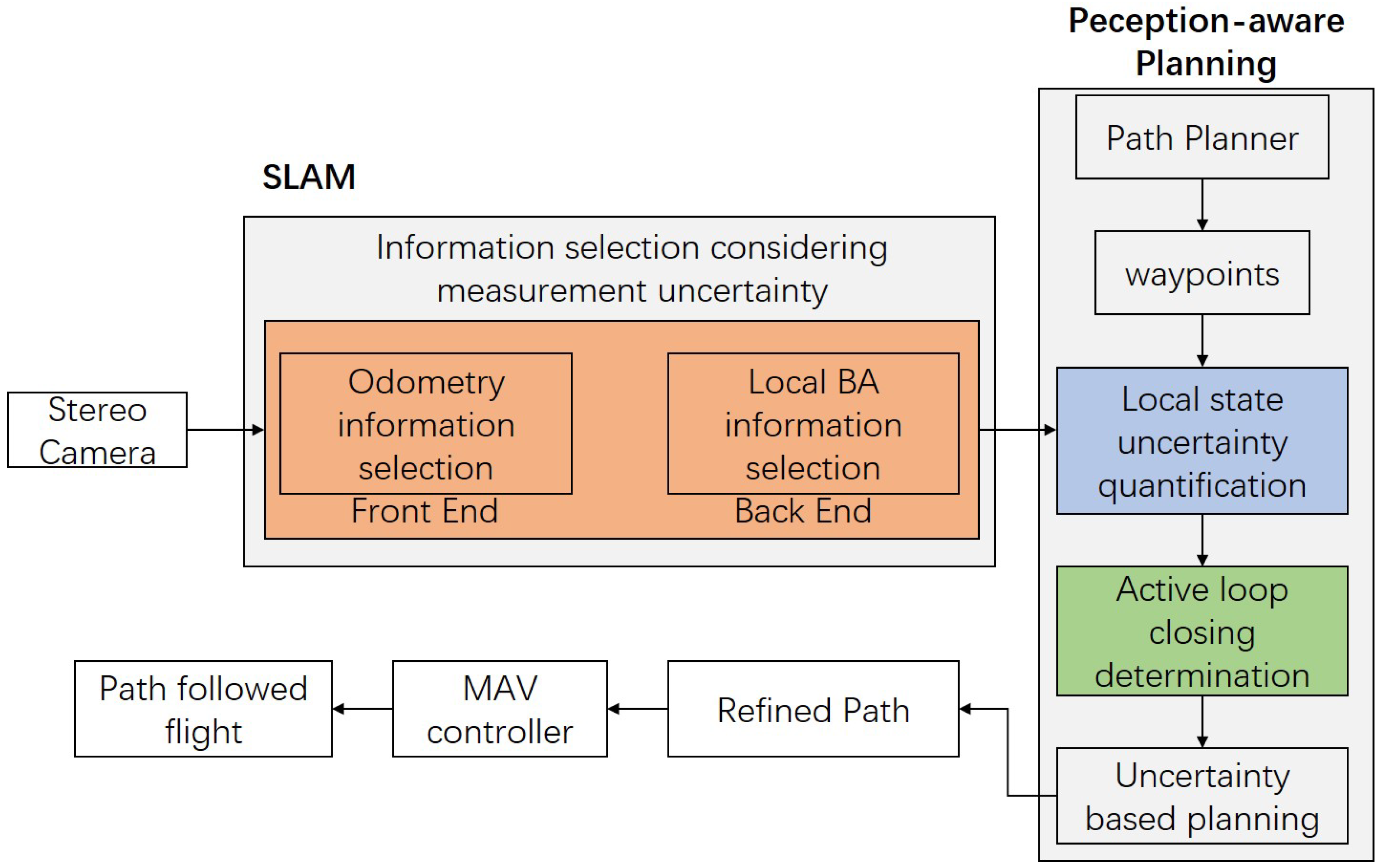
4.1. System Overview

The framework of the system can be seen in Figure 1. First, the measurement uncertainty based information selection is proposed in both front-end and back-end of the SLAM pipeline to find out measurements with high contribution, which improves computational efficiency. Second, the local state uncertainty based perception-aware active loop closing planning method is proposed to plan a trajectory that facilitates the improvement of localization accuracy. Different to our previous in [30], in this work, optimality criteria are introduced to quantify the uncertainty of the local state. Moreover, we define a generalized unary node to consider the poses and map points in the local BA as a whole state. Additionally, the binary edge connecting the states in the local BA becomes a generalized unary edge. The purpose is to fix the dimension of the state when calculating uncertainty and to avoid a sharp increase in the dimension of the Fisher Information Matrix due to the increase in nodes, which significantly improves the computational efficiency of the system.

4.2. Information Selection Considering Measurement Uncertainty

4.2.1. Odometry Information Selection Considering Measurement Uncertainty

In the front-end visual odometry, feature point matching is first carried out between the current image frame and the key frame. After the corresponding feature points are obtained, the least-squares problem shown in Equation (5) is constructed by taking the pose between two image frames as the state to be optimized, and the camera pose corresponding to the current image frame is optimized by the graph optimization method. As described in Section 3.1, in this optimization process, the node is the camera pose corresponding to the current image frame, and the edge is the unary edge composed of reprojection errors corresponding to a number of map points. In a MAV search and rescue scenario, the current image may match several features. The practice of constructing measurement based on the reprojection error of each feature point affects the computational efficiency of the front-end visual odometry in the case of many feature points. Therefore, an odometry information selection method considering measurement uncertainty is designed in this section. Firstly, based on the edges composed of the measurements from the matched feature points, the Fisher Information Matrix corresponding to that edge and the Cramér–Rao Lower Bound of uncertainty are calculated, and the uncertainty of that measurement is quantified according to the metric criterion in Section 3.4. Secondly, since the feature points are extracted from the ORB features with an image pyramid; the pyramid is divided into seven layers, and each layer corresponds to a different variance of the feature point positions. Considering that the image coordinates u and v of each feature point position are independent of each other, the uncertainty of the feature point position can be represented by the covariance matrix. The covariance is generally determined based on the pyramid level where the feature points are extracted. Specifically, when extracting ORB features, each level of the image pyramid is reduced to a scale of s. Following the framework of ORB-SLAM2 [26], we assume that the standard deviation of the $0th$ level is p pixels. Then, the covariance matrix of the reprojection error of a feature extracted at the $nth$ level of the pyramid can be expressed as follows.

$${\Sigma }_{\mathit{M}}={\left(s^n\times p\right)}^2\left[\begin{array}{cc}1\hfill & 0\hfill \\ 0\hfill & 1\hfill \end{array}\right]$$

(30)

The D-opt criterion is used to quantify the measurement uncertainty. Measurements with uncertainty greater than a certain threshold are filtered out in each layer based on Fisher Information and are not included in the process of pose optimization, because such measurements do not contribute much to the current pose estimation. The Fisher Information Matrix corresponding to this process is as follows.

$$I\left(\xi \right)={\left({\displaystyle \frac{\mathit{\partial }{e}_i}{\mathit{\partial }\xi }}\right)}^T{\Sigma }_{\left(u_i,v_i\right)}^{-1}{\displaystyle \frac{\mathit{\partial }{e}_i}{\mathit{\partial }\xi }}$$

(31)

where $\xi$ denotes camera pose.

By adopting the method above, the efficiency of front-end odometry pose estimation can be improved while ensuring localization accuracy. The process of odometry information selection algorithm considering measurement uncertainty is shown in Algorithm 1.

Algorithm 1 odometry information selection algorithm considering measurement uncertainty

Input:  initial pose $\xi$, set of edges $U_E$, coordinates of feature point positions $(u_i,v_i)$, variance of feature points ${\sigma }_j^2$, uncertainty quantification threshold $T{h}_{D-opt}$ Output:  set of selected edges $U_{Es}$ 1: Initialize $U_{Es}=⌀$  2: for all $e_i\in U_E$ do 3:    Determine the variance ${\sigma }_j^2$ according to the coordinates $(u_i,v_i)$ of the position of the feature point corresponding to $e_i$ 4:    Calculate the Fisher Information Matrix $I\left(\xi \right)$ and the Cramér-Rao Lower Bound $I^{-1}\left(\xi \right)$ for uncertainty following Equation (31) 5:    The D-opt criterion is used to calculate the uncertainty quantitative metric $m_{D-opt}$ of the measurement $e_i$ following Equation (29) 6:    if $m_{D-opt}<T{h}_{D-opt}$ then 7:        $U_{Es}=U_{Es}\cup \left\{e_i\right\}$ 8:    end if 9: end for

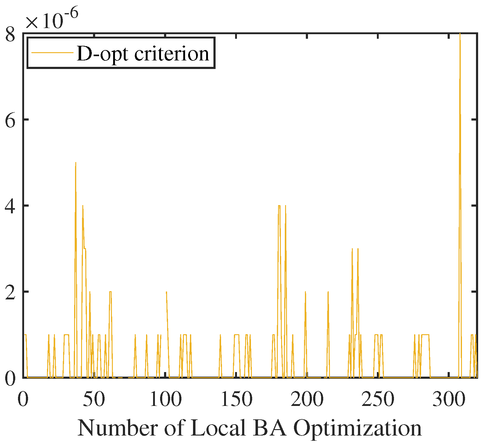
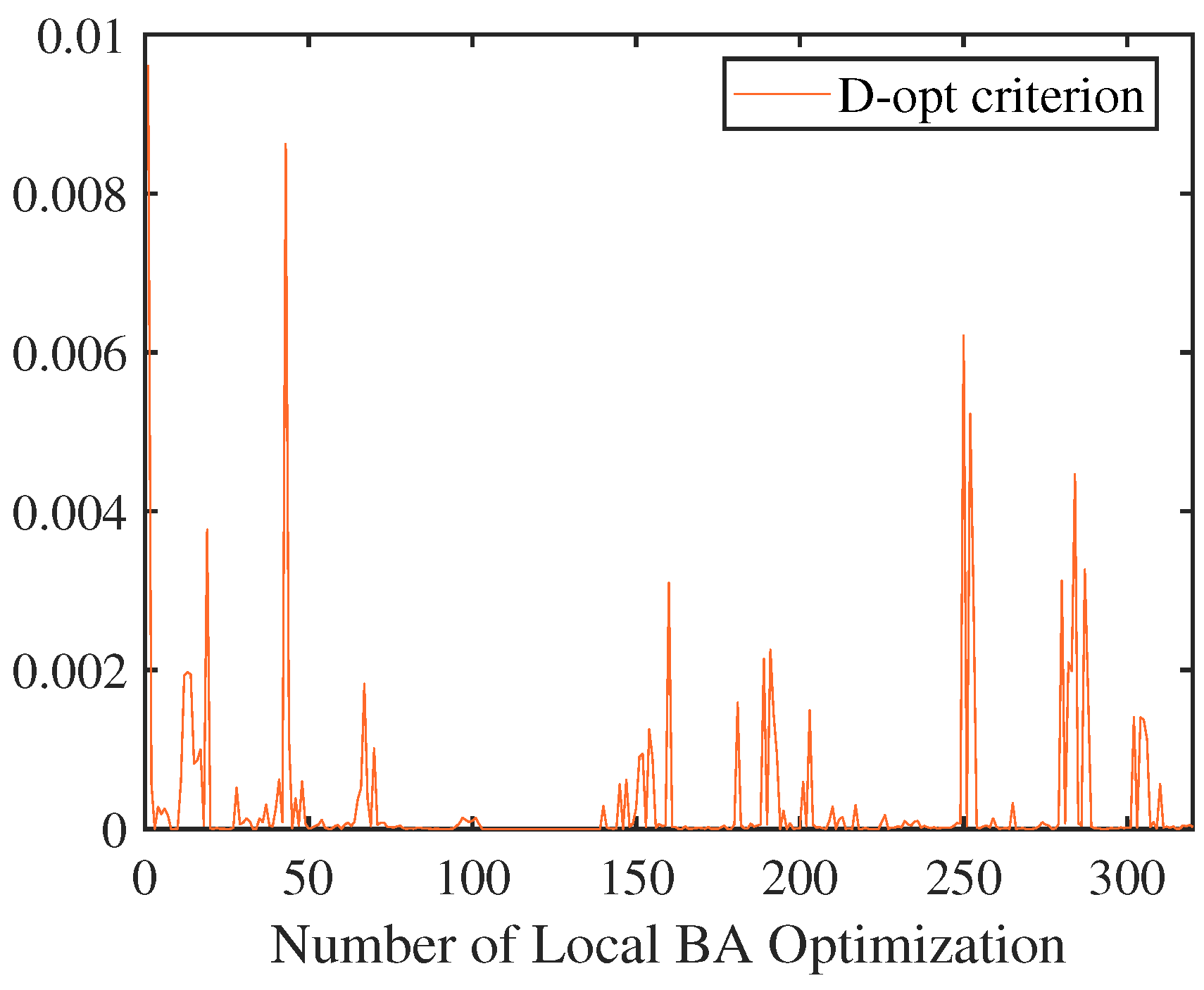
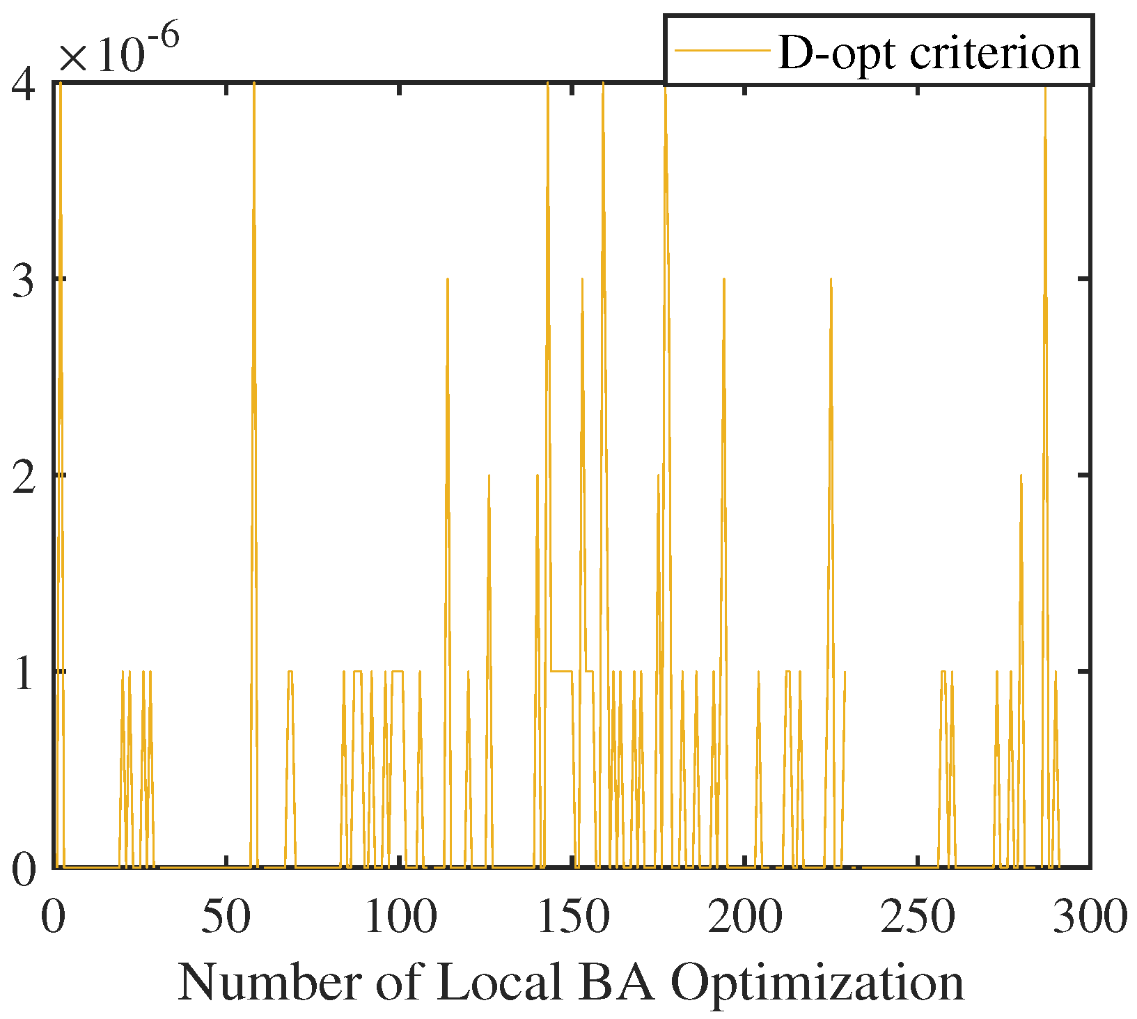
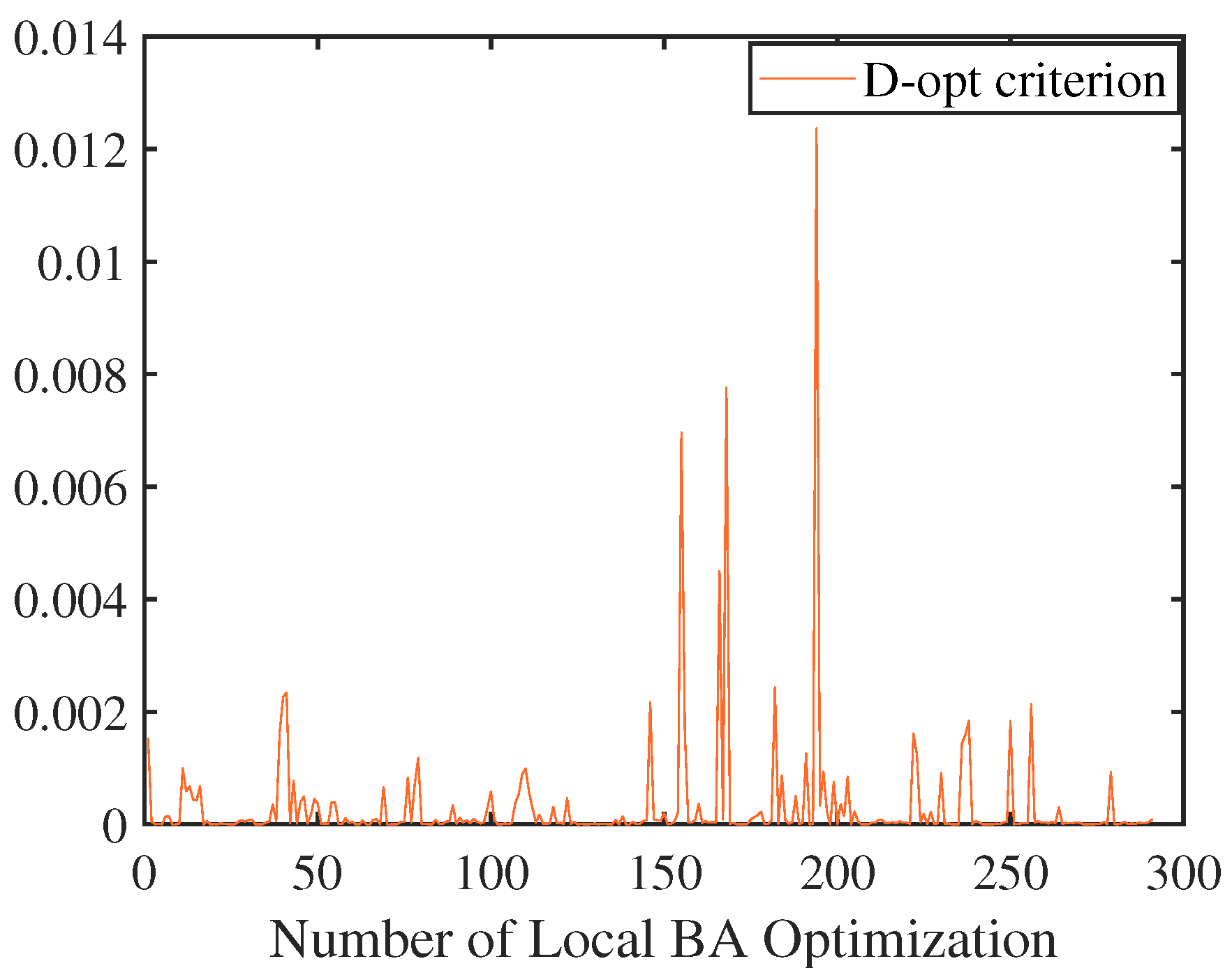
4.2.2. Local BA Information Selection Considering Measurement Uncertainty

The front-end odometry estimates the relative poses between the two image frames based on the feature points matched between the current image frame and the key frame, together with the reprojection error of the feature points. Further, the estimation of the current pose is achieved by means of dead reckoning. However, the localization error of this approach will inevitably accumulate gradually over time due to the presence of measurement noise. Therefore, when new keyframes appear, the bundle adjustment method is first adopted to optimize the local poses and map points so as to obtain more accurate poses and map information. As mentioned in Section 3.1, the optimization process optimizes both the map points and the camera poses. Considering that there are more measurements in the local BA, a local BA information selection method considering measurement uncertainty is proposed in this section. Among the numerous measurements, similar to Section 4.2.1, measurements with uncertainty greater than a certain threshold are filtered out based on the Fisher Information Matrix and the optimality criteria. Different to the situation in Section 4.2.1, a number of poses and map points are optimized at the same time; the uncertainties caused by the measurements for both the poses and the map points need to be considered simultaneously. The Fisher Information Matrix is as follows.

$$I\left({\xi }_j,P_k\right)={\left[\begin{array}{cc}{\left({\displaystyle \frac{\mathit{\partial }{e}_i}{\mathit{\partial }{\xi }_j}}\right)}^T{\Sigma }_{\left(u_k,v_k\right)}^{-1}{\displaystyle \frac{\mathit{\partial }{e}_i}{\mathit{\partial }{\xi }_j}}& {\left({\displaystyle \frac{\mathit{\partial }{e}_i}{\mathit{\partial }{\xi }_j}}\right)}^T{\Sigma }_{\left(u_k,v_k\right)}^{-1}{\displaystyle \frac{\mathit{\partial }{e}_i}{\mathit{\partial }{P}_k}}\\ {\left({\displaystyle \frac{\mathit{\partial }{e}_i}{\mathit{\partial }{P}_k}}\right)}^T{\Sigma }_{\left(u_k,v_k\right)}^{-1}{\displaystyle \frac{\mathit{\partial }{e}_i}{\mathit{\partial }{\xi }_j}}& {\left({\displaystyle \frac{\mathit{\partial }{e}_i}{\mathit{\partial }{P}_k}}\right)}^T{\Sigma }_{\left(u_k,v_k\right)}^{-1}{\displaystyle \frac{\mathit{\partial }{e}_i}{\mathit{\partial }{P}_k}}\end{array}\right]}_{9\times 9}$$

(32)

where, ${\xi }_j$ denotes camera pose, and $P_k$ denotes the spatial position of feature points. The above measurement information selection method can improve the efficiency of the calculation of camera poses and map point optimization in the process of local BA optimization. The process of local BA information selection algorithm considering measurement uncertainty is shown in Algorithm 2.

Algorithm 2 local BA information selection algorithm considering measurement uncertainty

Input:  initial pose and map point ${\xi }_j$$P_k$, set of edges $B_E$, coordinates of feature point in key frames $(u_k,v_k)$, variance of feature points ${\sigma }_l^2$, uncertainty quantification threshold $T{h}_{D-opt}$ Output:  set of selected edges $B_{Es}$ 1: Initialize $B_{Es}=⌀$ 2: for all $e_i\in U_E$ do 3:    Determine the variance ${\sigma }_l^2$ according to the coordinates $(u_k,v_k)$ of the position of the feature point corresponding to $e_i$ 4:    Calculate the Fisher Information Matrix $I({\xi }_j,P_k)$ and the Cramér-Rao Lower Bound $I^{-1}({\xi }_j,P_k)$ for uncertainty following Equation (32) 5:    The D-opt criterion is used to calculate the uncertainty quantitative metric $m_{D-opt}$ of the measurement $e_i$ following Equation (29) 6:    if $m_{D-opt}<T{h}_{D-opt}$ then 7:      $B_{Es}=B_{Es}\cup \left\{e_i\right\}$ 8:    end if 9: end for

4.3. Perception-Aware Active Loop Closing Planning Considering Local State Uncertainty

The method proposed in the previous section highlights the importance of Fisher Information in measurement information selection, and in this section, we explore the application of Fisher Information in planning and decision-making from the perspective of search and rescue MAV exploration and planning. The active loop closing planning method considering local state uncertainty (U-ALCP) is proposed in this section by utilizing Fisher Information and optimality criteria for the representation and quantification of uncertainty in local BA optimization, which is an active SLAM method further combining the SLAM algorithm and planning algorithm.

4.3.1. Definition of Generalized Unary Node and Generalized Unary Edge in Local BA

As can be seen from the description above, in the local BA optimization, the edge connecting the camera poses and the map feature points is a binary edge since the camera poses and map feature points are optimized simultaneously. With the continuous addition of key frames, there are more and more pose nodes and map points in the local map. When representing uncertainties with the Fisher Information Matrix, classifying poses and map points separately as states will cause the dimensionality of the Fisher Information Matrix to increase rapidly, resulting in an exponential increase in the computational burden. Therefore, in order to reduce the computational burden, in this section, all the states (i.e., camera pose, map feature points) in the local BA optimization are regarded as a whole, which is defined as a generalized node, and the binary edge connecting the camera pose and map feature points becomes a unary edge connecting the interior of the states, which is defined as a generalized unary edge in this work. The schematic diagram of generalized nodes and generalized unary edges is shown in Figure 2. In this way, the dimensionality of the Fisher Information Matrix, which represents the SLAM uncertainty, is fixed and is equal to the dimensionality of the camera poses together with the dimensionality of the map points. In this work, all the states in local BA optimization are considered as a whole when quantifying the uncertainty to decrease the computational burden. The local BA optimization process is not simplified when estimating pose; thus, the accuracy of the pose estimation can be guaranteed.

4.3.2. Uncertainty Representation of Local States

According to the definition of the generalized unary edge above, the Fisher Information Matrix is divided into the following two parts.

(1) Camera pose uncertainty

$$I{\left(\xi \right)}_{BA}=\sum _{i=1}^N{\left({\displaystyle \frac{\mathit{\partial }{e}_i}{\mathit{\partial }{\xi }_j}}\right)}^T{\Sigma }_{\left(u_k,v_k\right)}^{-1}{\displaystyle \frac{\mathit{\partial }{e}_i}{\mathit{\partial }{\xi }_j}}$$

(33)

(2) Map point uncertainty

$$I{\left(P\right)}_{BA}=\sum _{i=1}^N{\left({\displaystyle \frac{\mathit{\partial }{e}_i}{\mathit{\partial }{P}_k}}\right)}^T{\Sigma }_{\left(u_k,v_k\right)}^{-1}{\displaystyle \frac{\mathit{\partial }{e}_i}{\mathit{\partial }{P}_k}}$$

(34)

From Equations (33) and (34), the complete Fisher Information Matrix representing the local state uncertainty can be obtained as shown in Equation (35).

$$\begin{array}{cc}\hfill & I{(\xi ,P)}_{BA}=\hfill \\ \hfill & {\left[\begin{array}{cc}I{\left(\xi \right)}_{BA}& {\sum }_{i=1}^N{\left({\displaystyle \frac{\mathit{\partial }{e}_i}{\mathit{\partial }{\xi }_j}}\right)}^T{\Sigma }_{\left(u_k,v_k\right)}^{-1}{\displaystyle \frac{\mathit{\partial }{e}_i}{\mathit{\partial }{P}_k}}\\ {\sum }_{i=1}^N{\left({\displaystyle \frac{\mathit{\partial }{e}_i}{\mathit{\partial }{P}_k}}\right)}^T{\Sigma }_{\left(u_k,v_k\right)}^{-1}{\displaystyle \frac{\mathit{\partial }{e}_i}{\mathit{\partial }{\xi }_j}}& I{\left(P\right)}_{BA}\end{array}\right]}_{9\times 9}\hfill \end{array}$$

(35)

4.3.3. Active Loop Closing Strategy Considering Local State Uncertainty

The D-opt criterion is adopted to quantify the uncertainty of camera poses, map points, and the whole local state in local BA optimization, respectively. Also, the uncertainty of local maps can be analyzed. When the local state uncertainty at a certain moment is greater than a certain threshold, an active loop closing strategy is performed to further reduce the state uncertainty. The flow of the active loop closing planning algorithm considering local state uncertainty is shown in Algorithm 3. More detail about active loop closing, best node, and key way point selection can be found in our previous work [30].

Algorithm 3 Active loop closing planning algorithm considering local state uncertainty

Input:  best node $n_{best}$, initial pose and map point ${\xi }_j$$P_k$, set of selected edges $B_{Es}$, coordinates of feature point in key frames $(u_k,v_k)$, variance of feature points ${\sigma }_l^2$, uncertainty quantification threshold $T{h}_{D-opt}$ Output:  active loop closing flag $bFla{g}_{lc}$, planned path $ϵ$ 1: Select key waypoint according to $n_{best}$ 2: Save key waypoint as $w{p}_{key}$ 3: List $w{p}_{key}$ as candidate active loop closing waypoints 4: if $w{p}_{key}\ne ⌀$ then 5:    $bFla{g}_{lc}$ = true 6: end if 7: for all $e_i\in B_{Es}$ do 8:    Determine the variance ${\sigma }_l^2$ according to the coordinates $(u_k,v_k)$ of the position of the feature point corresponding to $e_i$ 9:    Calculate the Fisher Information Matrix $I{(\xi ,P)}_{BA}$ and the Cramér-Rao Lower Bound $I^{-1}{(\xi ,P)}_{BA}$ for uncertainty following Equation (35) 10:    The D-opt criterion is used to calculate the local state uncertainty quantitative metric $M_{D-opt}$ following Equation (29) 11: end for 12: if ($m_{D-opt}>T{h}_{D-opt}$ and $bFla{g}_{lc}=$ true) then 13:    Perform active loop closing planning to find the path $ϵ$ 14: end if

5. Results and Analysis

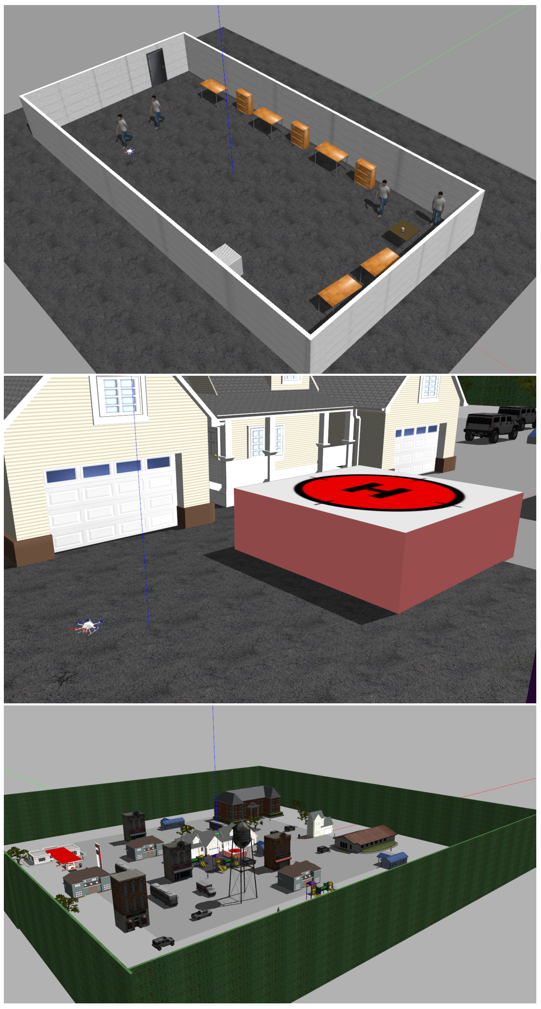
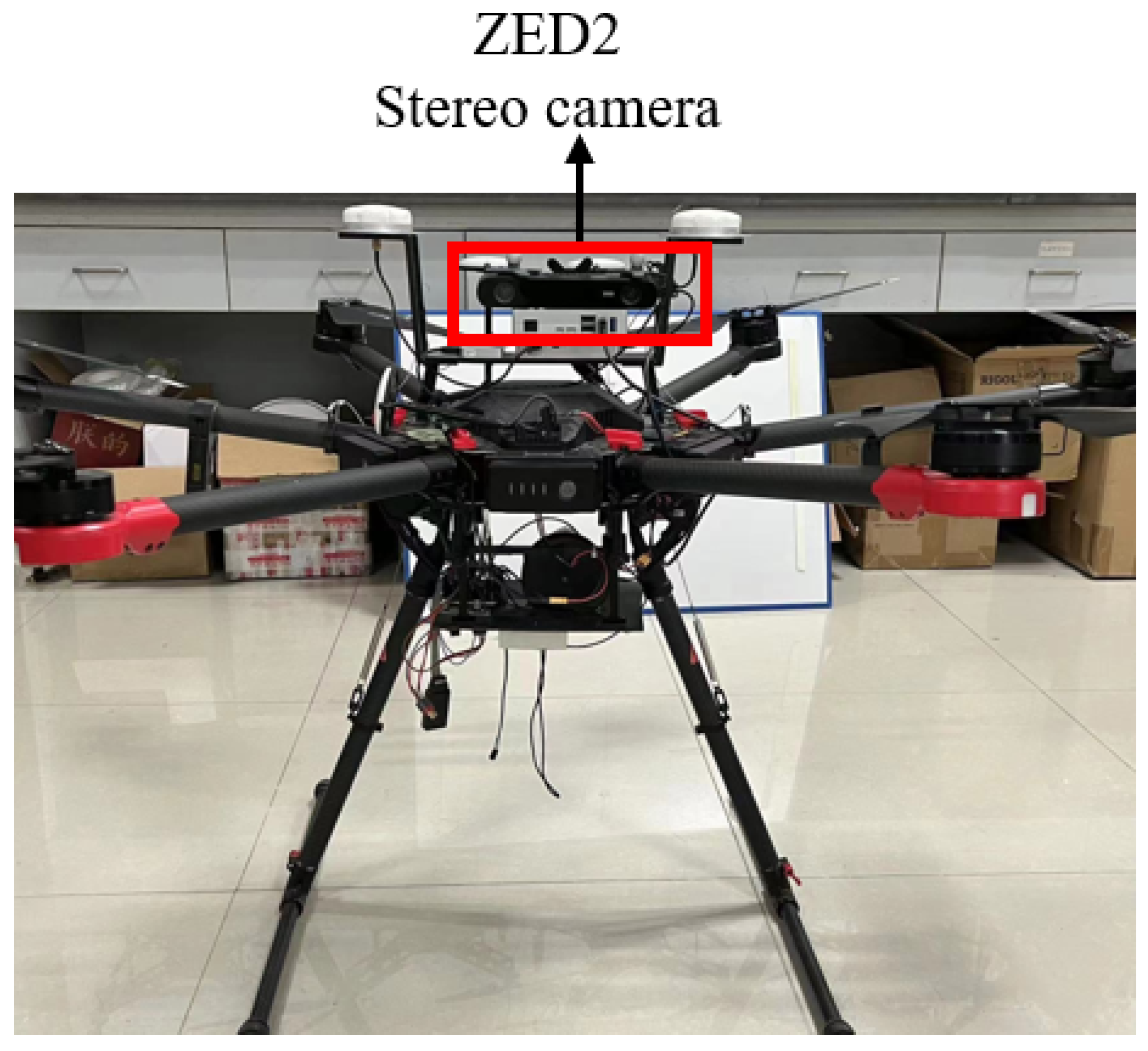
5.1. Experimental Settings and Sensors Configuration

In this section, the information selection method considering measurement uncertainty proposed in this work are evaluated. Moreover, the effects of camera pose uncertainty, map point uncertainty, and complete local state uncertainty on active loop closing planning are compared and analyzed in detail. For simulation environments, a flight simulation in different scales and environments is performed based on the Gazebo simulator [31] to test the real-time performance and localization accuracy of the proposed method. The RotorS simulator [32] equipped with the sensors of IMU and stereo camera is used to provide the parameters of the MAV. Both indoor and outdoor scenarios are shown in Figure 3, where the medium-scale scenario is part of the large-scale scenario. Moreover, DJI-M600 (DJI, Shenzhen, China) and the equipped sensor ZED2 stereo camera (StereoLabs, San Francisco, CA, USA) (Figure 4) are used for data collection in field tests. Algorithms in different scenarios were tested and verified on a computer with an Inter Core i7-10750H CPU at 2.6 GHz, a GTX1660Ti GPU, and 16 GB of RAM.

5.2. Results for Information Selection Considering Measurement Uncertainty

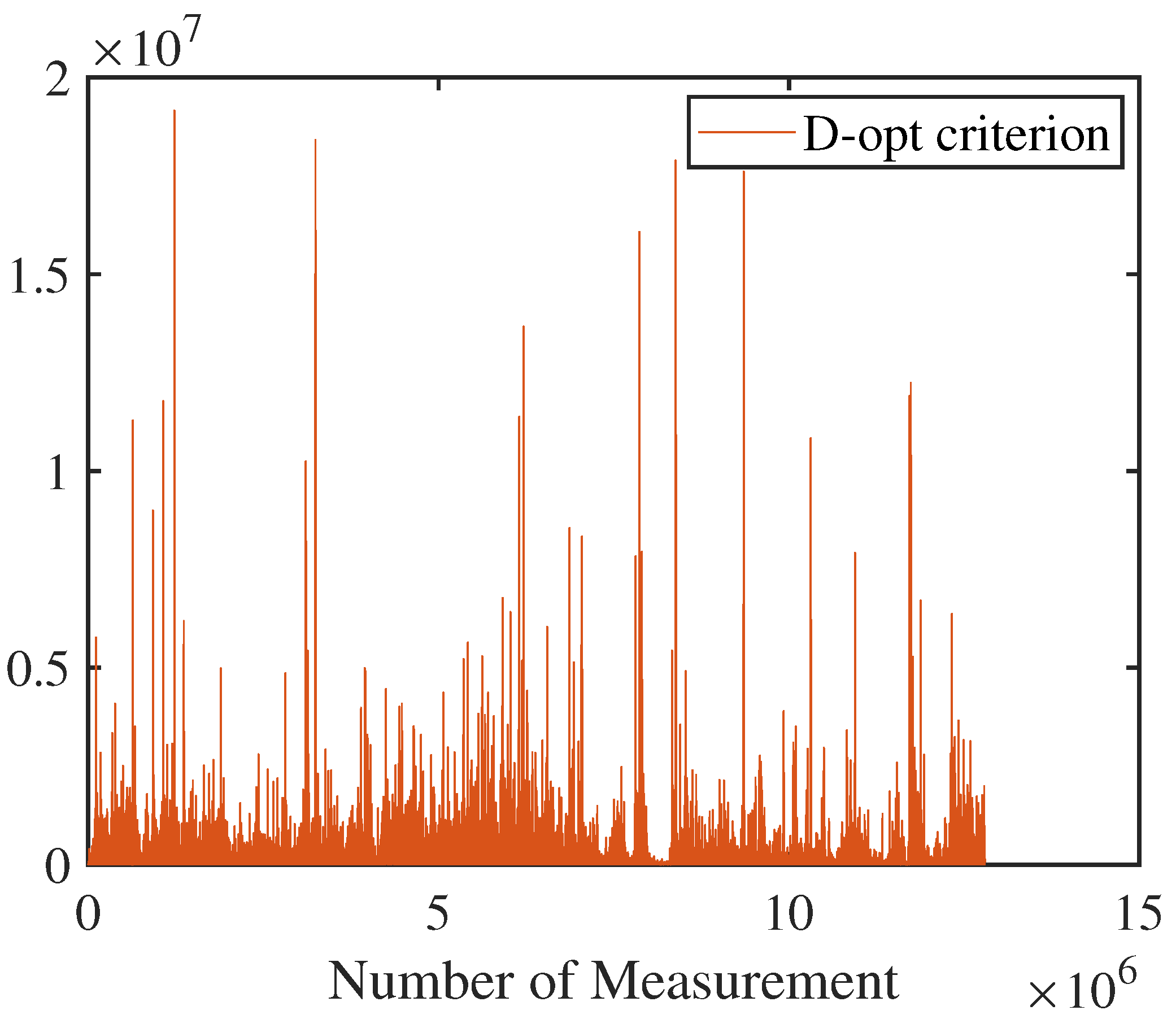
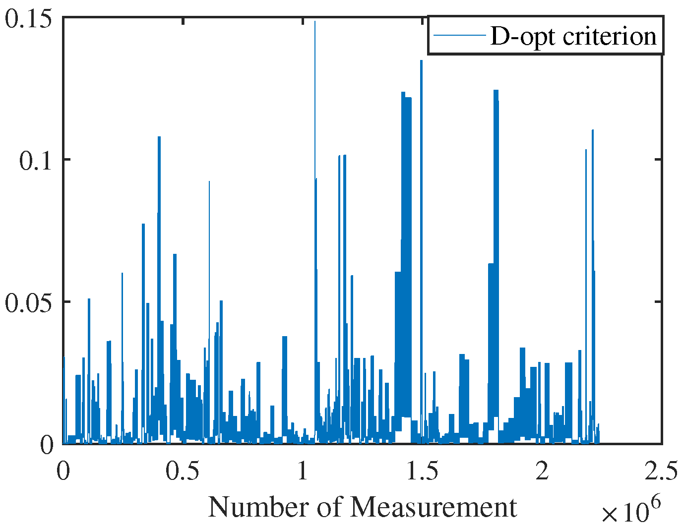
5.2.1. Visual Odometry Measurement Information Selection

In this section, validation of the visual odometry measurement information selection method is carried out with simulation data collected from Next-Best-View Planner (NBVP) [33] and Active Loop Closing Planner (ALCP) [30] planning methods. The methods proposed in this work that consider measurement and state uncertainty are denoted as U-NBVP and U-ALCP, respectively.

According to the uncertainty quantification metric, the appropriate threshold value can be determined, and the measurement over the threshold value will be discarded, which can improve the computing efficiency of the visual odometry tracking module. The threshold can be adjusted depending on the scenario. In this work, we first test NBVP and ALCP methods in different scenarios and then quantify the measurement uncertainty. Taking the small-scale scenario, for instance, the uncertainty quantification curves of the measurement information with NBVP and ALCP algorithms before information selection are shown in Figure 5 and Figure 6. The horizontal coordinates of the figure are the number of measurement information (number of edges) and the vertical coordinates are the quantitative metrics of the D-opt criterion. Subsequently, thresholds are selected based on the performance of existing algorithms for the proposed method in this work. Five times the mean value of the uncertainty metric was selected as the threshold value. Such a threshold selection strategy is able to eliminate some of the measurement information with high uncertainty without eliminating too many measurements, which could affect the accuracy of the pose estimation. Specifically, in scenarios with a priori information, the properties of the uncertainty quantitative metric can be selected according to the peak and mean value. In unknown scenarios without a priori information, the uncertainty quantitative metric can be determined based on the mean value of measurements during the initial stage of tracking process. Generally, the threshold value is chosen to be 5–8 times the mean value. The visual odometry measurement uncertainty quantification thresholds for measurement information selection in different scenarios are shown in

Table 1. Uncertainty quantification thresholds for odometry measurement information selection in different scenarios.

Scenarios	U-NBVP	U-ALCP
	Uncertainty Threshold	Uncertainty Threshold
small-scale	$1.5\times {10}^7$	$1\times {10}^7$
middle-scale	$4\times {10}^7$	$4\times {10}^7$
large-scale	$1\times {10}^8$	$1\times {10}^8$

. The time consumption of the tracking module before and after adopting the odometry information selection method in different scenarios is compared with the above thresholds, which is shown in

Table 2. Comparison of tracking time-consuming performance before and after the adoption of odometry informaiton selection method in different scenarios.

Scenarios	Method	Information Section	Median Tracking Time (ms)	Mean Tracking Time (ms)
small-scale	NBVP	×	48.68	50.33
	U-NBVP(ours)	✓	45.74	47.43
	ALCP	×	44.93	46.32
	U-ALCP(ours)	✓	44.08	45.72
medium-scale	NBVP	×	50.72	53.79
	U-NBVP(ours)	✓	48.80	50.90
	ALCP	×	49.34	52.15
	U-ALCP(ours)	✓	47.72	50.31
large-scale	NBVP	×	53.21	56.13
	U-NBVP(ours)	✓	50.76	54.01
	ALCP	×	52.28	55.83
	U-ALCP(ours)	✓	50.37	53.15

. A comparison of the absolute trajectory root mean square error (RMSE) and mean error in different scenarios can be seen in

Table 3. Comparison of absolute trajectory RMSE and mean error before and after odometry measurement information selection in different scenarios (v = 0.2 m/s).

Scenarios	Method	Information Selection	RMSE (m)	Mean (m)
small-scale	NBVP	×	3.25	2.56
	U-NBVP(ours)	✓	3.29	2.51
	ALCP	×	3.21	2.87
	U-ALCP(ours)	✓	3.21	2.88
medium-scale	NBVP	×	2.32	1.78
	U-NBVP(ours)	✓	2.35	1.76
	ALCP	×	1.00	0.91
	U-ALCP(ours)	✓	0.94	0.95
large-scale	NBVP	×	4.89	3.66
	U-NBVP(ours)	✓	4.86	3.70
	ALCP	×	3.45	3.49
	U-ALCP(ours)	✓	3.45	3.50

.

From the graphs above, we can find that after the adoption of the odometry measurement information selection method in different scenarios, the computing efficiency of the front-end odometry tracking module is improved. Meanwhile, the localization accuracy is equivalent to that before the information selection, as the contribution of the measurement information removed after the selection is relatively small.

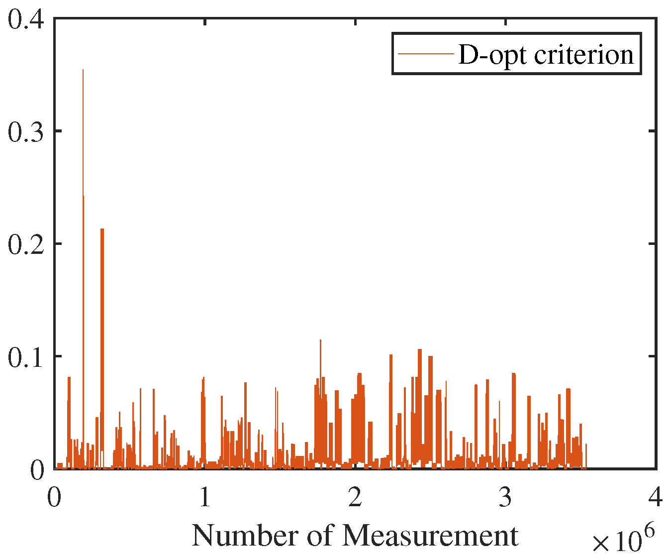
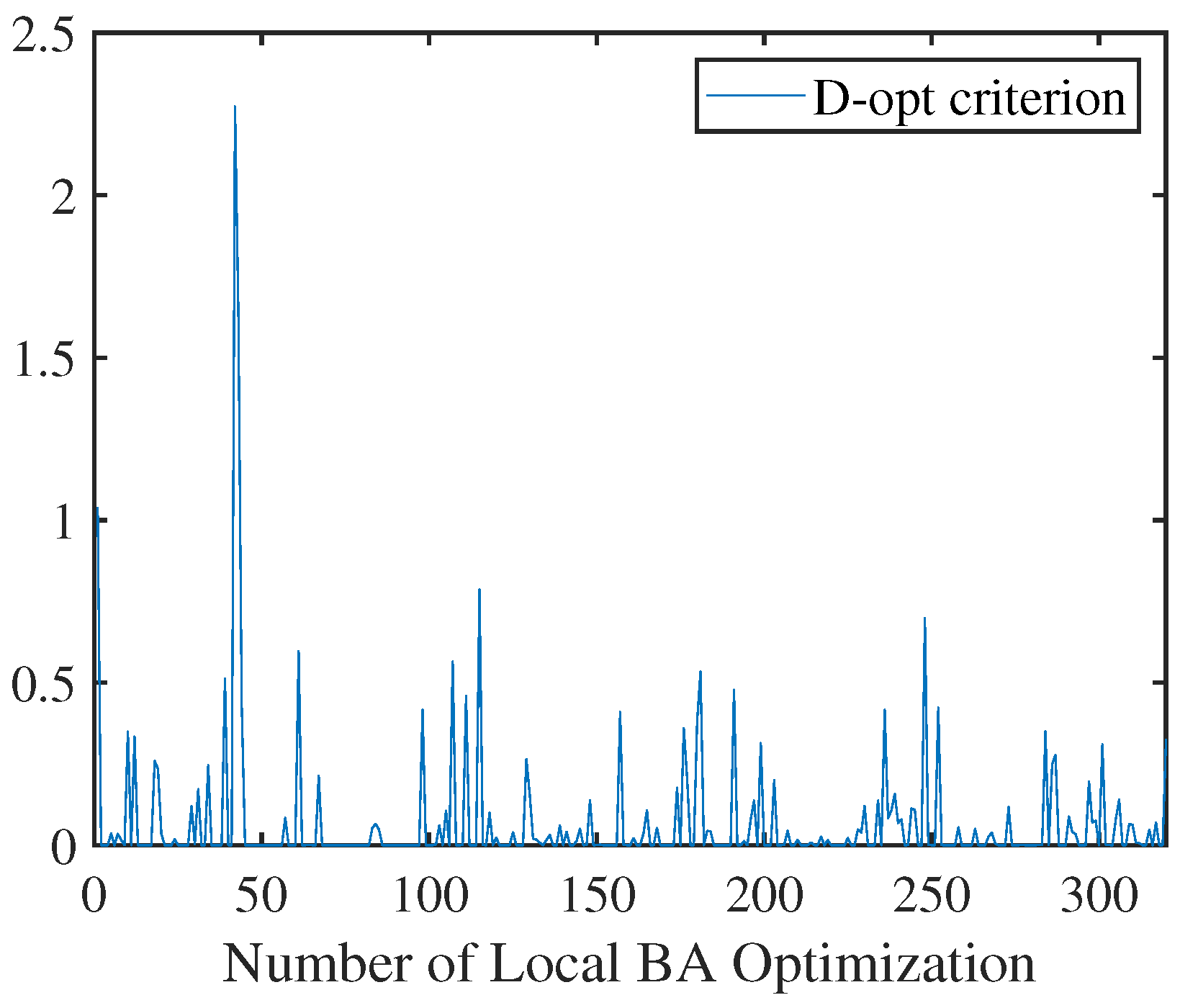
5.2.2. Local BA Measurement Information Selection

Similar to Section 5.2.1, validation of the local BA measurement information selection method is carried out with simulation data collected from NBVP and ALCP planning methods. Taking a small-scale scenario for instance, the uncertainty quantification curves of the measurement information with NBVP and ALCP algorithms before information selection are shown in Figure 7 and Figure 8. The horizontal coordinates of the figure are the number of measurement information (number of edges) and the vertical coordinates are the quantitative metrics of the D-opt criterion.

The selection strategy of the uncertainty threshold is consistent with Section 5.2.1. In this work, the local BA measurement uncertainty quantification thresholds for measurement information selection in different scenarios are shown in

Table 4. Uncertainty quantification thresholds for local BA measurement information selection in different scenarios.

Scenarios	U-NBVP	U-ALCP
	Uncertainty Threshold	Uncertainty Threshold
small-scale	0.1	0.1
middle-scale	2	2
large-scale	4.5	4.5

. The time-consuming performance of the tracking module before and after the adoption the local BA informaiton selection method in different scenarios is compared with the above thresholds, which is shown in

Table 5. Comparison of tracking time-consuming performance before and after the adoption of local BA information selection method in different scenarios.

Scenarios	Method	Information Selection	Median Tracking Time (ms)	Mean Tracking Time (ms)
small-scale	NBVP	×	105.78	157.65
	U-NBVP(ours)	✓	99.26	148.23
	ALCP	×	91.56	139.59
	U-ALCP(ours)	✓	80.26	120.02
medium-scale	NBVP	×	199.85	279.61
	U-NBVP(ours)	✓	184.20	270.62
	ALCP	×	159.82	227.05
	U-ALCP(ours)	✓	123.97	175.09
large-scale	NBVP	×	191.45	257.11
	U-NBVP(ours)	✓	169.49	201.20
	ALCP	×	186.92	203.04
	U-ALCP(ours)	✓	163.28	190.77

. A comparison of the absolute trajectory RMSE and mean error in different scenarios can be seen in

Table 6. Comparison of absolute trajectory RMSE and mean error before and after local BA measurement information selection in different scenarios (v = 0.2 m/s).

Scenarios	Method	Information Selection	RMSE (m)	Mean (m)
small-scale	NBVP	×	3.25	2.56
	U-NBVP(ours)	✓	3.26	2.56
	ALCP	×	3.21	2.87
	U-ALCP(ours)	✓	3.27	2.90
medium-scale	NBVP	×	2.32	1.78
	U-NBVP(ours)	✓	2.19	1.76
	ALCP	×	1.00	0.91
	U-ALCP(ours)	✓	0.79	0.85
large-scale	NBVP	×	4.89	3.66
	U-NBVP(ours)	✓	4.82	3.70
	ALCP	×	3.45	3.49
	U-ALCP(ours)	✓	3.43	3.55

.

The comparison of the time-consuming performance and localization accuracy of the local BA optimization before and after the measurement information selection method in the graphs above indicates that after the adoption of the local BA optimization measurement information selection method in different scenarios, the computing efficiency of the back-end local BA optimization is improved. Meanwhile, the localization accuracy is equivalent to that before information selection.

5.3. Results for Active Loop Closing Planning Considering Local State Uncertainty

In this section, the local state uncertainty of the collected data is first quantified and analyzed. On the basis of the analysis results, the uncertainty threshold for performing active loop closing planning is determined. The active loop closing planning method considering local state uncertainty proposed in Section 4.3 is validated in the same scenario, and the effects of pose uncertainty and map point uncertainty on the active loop closing strategy and localization results are analyzed in detail.

Figure 9, Figure 10 and Figure 11 show the quantification curves of the pose uncertainty, map point uncertainty, and state uncertainty considering both pose and map feature points, for small-scale scenarios with the NBVP method. Similarly, Figure 12, Figure 13 and Figure 14 show the curves with ALCP method.

5.4. Field Tests

To further analyze the spread of localization error when the active loop closing is not available, data collection and localization error analysis were conducted in the corridor of the building using DJI-M600 and stereo visual sensor ZED2. Due to the specificity of the building corridor structure, the algorithm is verified by performing active loop closing and not performing active loop closing at the turnoffs of the building corridor, respectively. The curves for the two sets of tests are shown in Figure 15 below. The green curve in the figure indicates the localization trajectory without active loop closing, and the blue one indicates the localization trajectory with active loop closing. The details of the test method are as follows.

In the first group of tests without active loop closing, the end point and the starting point are separated by 55 square bricks with a side length of 60 cm, so the reference value of the distance between the starting point and the end point is 33 m. In the second set of tests, the building turnoff was closer to the starting point, so it returned to the starting point for an active loop closing, with a reference value of 0 m for the distance between the starting point and the end point. The estimated value of the distance between the end point and the starting point of the first group is 41.17 m, with an error of 8.17 m. The distance of movement was about 177 m, and the percentage of error at the end point is 4.61%. Meanwhile, the estimated value of the distance between the end point and the starting point of the first group is 3.31 m, with an error of 3.31 m. The distance of movement was about 210 m, and the percentage of error at the end point is 1.58%. Therefore, this test verifies that the adoption of active loop closing can effectively slow down the error spread, which is good for the improvement of localization accuracy.

5.5. Discussion

On the basis of the uncertainty quantification curves in Figure 9, Figure 10, Figure 11, Figure 12, Figure 13 and Figure 14, the following two aspects can be discussed in detail. On one hand, in terms of the estimated state, there are several points with large values in the curve when considering part of the state (camera poses or map points) separately or considering the state uncertainty of camera poses and map points simultaneously, which means that the state uncertainty of the local map is relatively large after local BA optimization. Thus, active loop closing planning can be performed at this point. On the other hand, in terms of the planning strategy, the uncertainty is not significantly reduced after the adoption of the ALCP method if only the uncertainty quantification metrics of the camera or map feature points are considered. However, the uncertainty of the camera poses and map points (Figure 14) is smaller when compared to the NBVP method (Figure 11). Although there are still a small number of curve points with high uncertainty, most of the uncertainty is relatively small. Moreover, for the four uncertainty peaks that occur between the 150th and 200th optimizations in Figure 14, the number of uncertainty peaks can be further reduced by using the local state uncertainty-based active loop closing strategy presented in this work.

The above analysis shows that after the active loop closing planning, the uncertainty of local poses and map feature points as a whole tends to decrease more obviously than that of simply considering the camera or map feature points; the reason is that the local BA optimization integrates all the states to be optimized and optimizes them as a whole. Therefore, in the validation of the local state uncertainty based active loop closing planning method proposed in this paper, both the pose and map point uncertainties will be considered, and the overall uncertainty quantification metric will be applied as the reference for active loop closing planning.

Similar to our previous work in [30], when adopting local state uncertainty based active loop closing strategy, it is necessary to determine the uncertainty quantification threshold and then perform active loop closing planning when the uncertainty is greater than the threshold. Different to [30], in this work, we include an uncertainty evaluation criterion in deciding whether active loop closing is required. The D-opt criterion is used for uncertainty evaluation in this work. Five times the mean value of the uncertainty metric was selected as the threshold value. In unknown scenarios without a priori information, the uncertainty quantitative metric can be determined based on the mean value of measurements during the initial stage of exploration process. Generally, the threshold value is chosen to be 5–8 times the mean value. Such a threshold selection strategy enables active loop closing planning when uncertainty is high, while not being too frequent to compromise exploration efficiency. Hence, the uncertainty quantification thresholds used for active loop closing planning are shown in

Table 7. Uncertainty quantification thresholds used for active loop closing planning in different scenarios.

Scenarios	U-NBVP	U-ALCP
	Uncertainty Threshold	Uncertainty Threshold
small-scale	0.005	0.004
middle-scale	0.015	0.01
large-scale	0.18	0.15

. A comparison of the absolute trajectory RMSE and mean error in different scenarios with the adoption of the active loop closing strategy is shown in

Table 8. Comparison of absolute trajectory RMSE and mean error before and after the adoption of active loop closing strategy in different scenarios (v = 0.2 m/s).

Scenarios	Method	Active Loop Closing	Uncertainty Quantification	RMSE (m)	Mean (m)
small-scale	NBVP	×	×	3.25	2.56
	U-NBVP(ours)	✓	✓	3.23	2.51
	ALCP	✓	×	3.21	2.87
	U-ALCP(ours)	✓	✓	3.21	2.88
medium-scale	NBVP	×	×	2.32	1.78
	U-NBVP(ours)	✓	✓	2.19	1.67
	ALCP	✓	×	1.00	0.91
	U-ALCP(ours)	✓	✓	0.79	0.85
large-scale	NBVP	×	×	4.89	3.66
	U-NBVP(ours)	✓	✓	4.33	3.54
	ALCP	✓	×	3.45	3.49
	U-ALCP(ours)	✓	✓	3.18	3.36

.

From the above diagram, we can find that, on one hand, the uncertainty thresholds vary in different scenarios, when adopting the local state uncertainty-based method for active loop closing planning. Generally speaking, the larger the scale of the scenario, the larger the state uncertainty, which needs to be selected adaptively according to the practical application scenarios. On the other hand, the adoption of the uncertainty quantification metric makes the uncertainty further reduced and the localization accuracy further improved during the MAV search and rescue process.

6. Conclusions

A visual active SLAM method considering measurement and state uncertainty for space exploration with a stereo camera is presented in this work. The Cramér–Rao Lower Bound for the localization uncertainty of the stereo visual SLAM system is derived with the benefit of the Fisher Information Matrix. The optimality criteria are introduced as a quantification metric to evaluate the pose and map point uncertainty in our stereo visual SLAM system. On this basis, to further improve the efficiency of the algorithm, an odometry information selection method considering measurement uncertainty is designed at the front end of the SLAM system, and a local BA optimization information selection method is designed at the back end to pick out the measurements with small uncertainty for localization and mapping, which improves the computational efficiency of the system while ensuring the localization accuracy. Moreover, according to the uncertainty of quantified local poses and map points, an active loop closing planning method considering local state uncertainty is proposed to exploit the uncertainty in assisting the space exploration and decision-making of search and rescue MAVs. Finally, the effectiveness of the method proposed in this work is verified in several challenging scenarios, which provides a new idea for the application of uncertainty evaluation in active SLAM. In future work, we could derive the measurement uncertainty representation under different noise models. Moreover, multi-MAVs active SLAM could be considered to further improve the performance of the system in complex scenarios.

References

1. Wang, X.; Zheng, S.; Lin, X.; Zhu, F. Improving RGB-D SLAM accuracy in dynamic environments based on semantic and geometric constraints. Measurement 2023, 217, 113084. [Google Scholar] [CrossRef]
2. Niroui, F.; Zhang, K.; Kashino, Z.; Nejat, G. Deep reinforcement learning robot for search and rescue applications: Exploration in unknown cluttered environments. IEEE Robot. Autom. Lett. 2019, 4, 610–617. [Google Scholar] [CrossRef]
3. Xia, L.; Meng, D.; Zhang, J.; Zhang, D.; Hu, Z. Visual-Inertial Simultaneous Localization and Mapping: Dynamically Fused Point-Line Feature Extraction and Engineered Robotic Applications. IEEE Trans. Instrum. Meas. 2022, 71, 5019211. [Google Scholar] [CrossRef]
4. Li, J.; Zhao, J.; Kang, Y.; He, X.; Ye, C.; Sun, L. Dl-slam: Direct 2.5 d lidar slam for autonomous driving. In Proceedings of the 2019 IEEE Intelligent Vehicles Symposium (IV), Paris, France, 9–12 June 2019; pp. 1205–1210. [Google Scholar]
5. Cheng, J.; Zhang, L.; Chen, Q.; Hu, X.; Cai, J. Map aided visual-inertial fusion localization method for autonomous driving vehicles. Measurement 2023, 221, 113432. [Google Scholar] [CrossRef]
6. Zhang, D.; Shen, Y.; Lu, J.; Jiang, Q.; Zhao, C.; Miao, Y. IPR-VINS: Real-time monocular visual-inertial SLAM with implicit plane optimization. Measurement 2024, 226, 114099. [Google Scholar] [CrossRef]
7. Jacobson, A.; Zeng, F.; Smith, D.; Boswell, N.; Peynot, T.; Milford, M. Semi-supervised slam: Leveraging low-cost sensors on underground autonomous vehicles for position tracking. In Proceedings of the 2018 IEEE/RSJ International Conference on Intelligent Robots and Systems (IROS), Madrid, Spain, 1–5 October 2018; pp. 3970–3977. [Google Scholar]
8. Chen, Y.; Huang, S.; Fitch, R. Active SLAM for mobile robots with area coverage and obstacle avoidance. IEEE/Asme Trans. Mechatronics 2020, 25, 1182–1192. [Google Scholar] [CrossRef]
9. Norbelt, M.; Luo, X.; Sun, J.; Claude, U. UAV Localization in Urban Area Mobility Environment Based on Monocular VSLAM with Deep Learning. Drones 2025, 9, 171. [Google Scholar] [CrossRef]
10. Zhou, B.; Li, C.; Chen, S.; Xie, D.; Yu, M.; Li, Q. ASL-SLAM: A LiDAR SLAM with Activity Semantics-Based Loop Closure. IEEE Sens. J. 2023, 23, 13499–13510. [Google Scholar] [CrossRef]
11. Kim, D.; Lee, B.; Sung, S. Design and Verification of Observability-Driven Autonomous Vehicle Exploration Using LiDAR SLAM. Aerospace 2024, 11, 120. [Google Scholar] [CrossRef]
12. Feder, H.J.S.; Leonard, J.J.; Smith, C.M. Adaptive mobile robot navigation and mapping. Int. J. Robot. Res. 1999, 18, 650–668. [Google Scholar] [CrossRef]
13. Carrillo, H.; Reid, I.; Castellanos, J.A. On the comparison of uncertainty criteria for active SLAM. In Proceedings of the 2012 IEEE International Conference on Robotics and Automation, St Paul, MN, USA, 14–18 May 2012; pp. 2080–2087. [Google Scholar]
14. Bonetto, E.; Goldschmid, P.; Pabst, M.; Black, M.J.; Ahmad, A. iRotate: Active visual SLAM for omnidirectional robots. Robot. Auton. Syst. 2022, 154, 104102. [Google Scholar] [CrossRef]
15. Rodríguez-Arévalo, M.L.; Neira, J.; Castellanos, J.A. On the importance of uncertainty representation in active SLAM. IEEE Trans. Robot. 2018, 34, 829–834. [Google Scholar] [CrossRef]
16. Placed, J.A.; Castellanos, J.A. Fast Autonomous Robotic Exploration Using the Underlying Graph Structure. In Proceedings of the 2021 IEEE/RSJ International Conference on Intelligent Robots and Systems (IROS), Prague, Czech Republic, 27 September–1 October 2021; pp. 6672–6679. [Google Scholar]
17. Chen, Y.; Huang, S.; Zhao, L.; Dissanayake, G. Cramér–Rao bounds and optimal design metrics for pose-graph SLAM. IEEE Trans. Robot. 2021, 37, 627–641. [Google Scholar] [CrossRef]
18. Carlone, L.; Du, J.; Kaouk Ng, M.; Bona, B.; Indri, M. Active SLAM and exploration with particle filters using Kullback-Leibler divergence. J. Intell. Robot. Syst. 2014, 75, 291–311. [Google Scholar] [CrossRef]
19. Yuan, J.; Zhu, S.; Tang, K.; Sun, Q. ORB-TEDM: An RGB-D SLAM Approach Fusing ORB Triangulation Estimates and Depth Measurements. IEEE Trans. Instrum. Meas. 2022, 71, 5006315. [Google Scholar] [CrossRef]
20. Carlone, L.; Karaman, S. Attention and anticipation in fast visual-inertial navigation. IEEE Trans. Robot. 2018, 35, 1–20. [Google Scholar] [CrossRef]
21. Murali, V. Perception-Aware Planning for Differentially Flat Robots. Ph.D. Thesis, Massachusetts Institute of Technology, Cambridge, MA, USA, 2024. [Google Scholar]
22. Sun, G.; Zhang, X.; Liu, Y.; Wang, H.; Zhang, X.; Zhuang, Y. Topology-Guided Perception-Aware Receding Horizon Trajectory Generation for UAVs. In Proceedings of the 2023 IEEE/RSJ International Conference on Intelligent Robots and Systems (IROS), Detroit, MI, USA, 1–5 October 2023; pp. 3070–3076. [Google Scholar]
23. Chen, X.; Zhang, Y.; Zhou, B.; Shen, S. APACE: Agile and Perception-Aware Trajectory Generation for Quadrotor Flights. arXiv 2024, arXiv:2403.08365. [Google Scholar]
24. Sun, G.; Zhang, X.; Liu, Y.; Zhang, X.; Zhuang, Y. Safety-Driven and Localization Uncertainty-Driven Perception-Aware Trajectory Planning for Quadrotor Unmanned Aerial Vehicles. IEEE Trans. Intell. Transp. Syst. 2024, 25, 8837–8848. [Google Scholar] [CrossRef]
25. Takemura, R.; Ishigami, G. Perception-and-Energy-aware Motion Planning for UAV using Learning-based Model under Heteroscedastic Uncertainty. In Proceedings of the 2024 IEEE International Conference on Robotics and Automation (ICRA), Yokohama, Japan, 13–17 May 2024; pp. 10103–10109. [Google Scholar]
26. Mur-Artal, R.; Tardós, J.D. Orb-slam2: An open-source slam system for monocular, stereo, and rgb-d cameras. IEEE Trans. Robot. 2017, 33, 1255–1262. [Google Scholar] [CrossRef]
27. Pázman, A. Foundations of Optimum Experimental Design; Springer: Berlin/Heidelberg, Germany, 1986. [Google Scholar]
28. Zhang, Z.; Scaramuzza, D. Beyond point clouds: Fisher information field for active visual localization. In Proceedings of the 2019 International Conference on Robotics and Automation (ICRA), Montreal, QC, Canada, 20–24 May 2019; pp. 5986–5992. [Google Scholar]
29. Kiefer, J. General equivalence theory for optimum designs (approximate theory). Ann. Stat. 1974, 2, 849–879. [Google Scholar] [CrossRef]
30. Zhao, Y.; Xiong, Z.; Zhou, S.; Wang, J.; Zhang, L.; Campoy, P. Perception-Aware Planning for Active SLAM in Dynamic Environments. Remote Sens. 2022, 14, 2584. [Google Scholar] [CrossRef]
31. Koenig, N.; Howard, A. Design and use paradigms for gazebo, an open-source multi-robot simulator. In Proceedings of the 2004 IEEE/RSJ International Conference on Intelligent Robots and Systems (IROS) (IEEE Cat. No. 04CH37566), Sendai, Japan, 28 September–2 October 2004; Volume 3, pp. 2149–2154. [Google Scholar]
32. Furrer, F.; Burri, M.; Achtelik, M.; Siegwart, R. Rotors—A modular gazebo mav simulator framework. In Robot Operating System (ROS); Springer: Berlin/Heidelberg, Germany, 2016; pp. 595–625. [Google Scholar]
33. Bircher, A.; Kamel, M.; Alexis, K.; Oleynikova, H.; Siegwart, R. Receding horizon “next-best-view” planner for 3d exploration. In Proceedings of the 2016 IEEE International Conference on Robotics and Automation (ICRA), Stockholm, Sweden, 16–21 May 2016; pp. 1462–1468. [Google Scholar]
Figure 1. Framework of system.
Aerospace 12 00642 g001
Figure 2. Schematic diagram of generalized nodes and generalized unary edges.The orange circles are nodes that indicate position of map points, the blue triangles are nodes that indicate camera poses, the dotted lines are generalized unary edges that indicate relative pose error, and the dashed lines are generalized unary edges that indicate reprojection error.
Aerospace 12 00642 g002
Figure 3. Small-scale (top), middle-scale (middle), and large-scale (bottom) scenarios.
Aerospace 12 00642 g003
Figure 4. DJI-M600 for field tests.
Aerospace 12 00642 g004
Figure 5. Visual odometry measurement uncertainty quantification curve (small-scale, NBVP).
Aerospace 12 00642 g005
Figure 6. Visual odometry measurement uncertainty quantification curve (small-scale, ALCP).
Aerospace 12 00642 g006
Figure 7. Local BA measurement uncertainty quantification curve (small-scale, NBVP).
Aerospace 12 00642 g007
Figure 8. Local BA measurement uncertainty quantification curve (small-scale, ALCP).
Aerospace 12 00642 g008
Figure 9. Local pose uncertainty quantification curve (small-scale, NBVP).
Aerospace 12 00642 g009
Figure 10. Local map point uncertainty quantification curve (small-scale, NBVP).
Aerospace 12 00642 g010
Figure 11. Local pose and map point uncertainty quantification curve (small-scale, NBVP).
Aerospace 12 00642 g011
Figure 12. Local pose uncertainty quantification curve (small-scale, ALCP).
Aerospace 12 00642 g012
Figure 13. Local map point uncertainty quantification curve (small-scale, ALCP).
Aerospace 12 00642 g013
Figure 14. Local pose and map point uncertainty quantification curve (small-scale, ALCP).
Aerospace 12 00642 g014
Figure 15. Trajectory with/without active loop closing in field test.
Aerospace 12 00642 g015