Resolving Non-Proportional Frequency Components in Rotating Machinery Signals Using Local Entropy Selection Scaling–Reassigning Chirplet Transform

Abstract

Under complex operating conditions, vibration signals from rotating machinery often exhibit non-stationary characteristics with non-proportional and closely spaced instantaneous frequency (IF) components. Traditional time–frequency analysis (TFA) methods struggle to accurately extract such features due to energy leakage and component mixing. In response to these issues, an enhanced time–frequency analysis approach, termed Local Entropy Selection Scaling–Reassigning Chirplet Transform (LESSRCT), has been developed to improve the representation accuracy for complex non-stationary signals. This approach constructs multi-channel time–frequency representations (TFRs) by introducing multiple scales of chirp rates (CRs) and utilizes a Rényi entropy-based criterion to adaptively select multiple optimal CRs at the same time center, enabling accurate characterization of multiple fundamental components. In addition, a frequency reassignment mechanism is incorporated to enhance energy concentration and suppress spectral diffusion. Extensive validation was conducted on a representative synthetic signal and three categories of real-world data—bat echolocation, inner race bearing faults, and wind turbine gearbox vibrations. In each case, the proposed LESSRCT method was compared against SBCT, GLCT, CWT, SET, EMCT, and STFT. On the synthetic signal, LESSRCT achieved the lowest Rényi entropy of 13.53, which was 19.5% lower than that of SET (16.87) and 35% lower than GLCT (18.36). In the bat signal analysis, LESSRCT reached an entropy of 11.53, substantially outperforming CWT (19.91) and SBCT (15.64). For bearing fault diagnosis signals, LESSRCT consistently achieved lower entropy across varying SNR levels compared to all baseline methods, demonstrating strong noise resilience and robustness. The final case on wind turbine signals demonstrated its robustness and computational efficiency, with a runtime of 1.31 s and excellent resolution. These results confirm that LESSRCT delivers robust, high-resolution TFRs with strong noise resilience and broad applicability. It holds strong potential for precise fault detection and condition monitoring in domains such as aerospace and renewable energy systems.

1. Introduction

As the aerospace industry continues to evolve, the reliability and safety of aerospace equipment are facing increasingly stringent requirements. Fault detection technology [1,2], as a crucial approach for maintaining equipment reliability, has made significant progress in recent years. For example, the defect diagnosis technique targeting liquid rocket propulsion systems based on Genetic Algorithm-optimized Least Squares Support Vector Regression (GA-LSSVR) has significantly enhanced the adaptability of fault detection by optimizing the parameters of the support vector machine [3]. Meanwhile, deep learning-based methods have gradually become mainstream. For instance, the use of one-dimensional Convolutional Neural Networks (1D-CNNs) combined with attention mechanisms has further improved the precision of fault detection [4].

Within the domain of rotating machinery, research on fault detection technology has also advanced rapidly. Taking planetary gearboxes as a typical example, some scholars have proposed a method utilizing an enhanced Complete Ensemble Empirical Mode Decomposition (ICEEMD) and information entropy in the time–frequency domain. By decomposing vibration signals and calculating the entropy of each intrinsic mode function (IMF), this method effectively extracts fault features [5]. For bearing fault diagnosis, a method combining Clustered Federated Learning (CFL) with self-attention mechanisms has been proposed. This method improves the generalization ability and diagnostic accuracy of the model by collaborative training among multiple clients and leveraging the similarity of data distributions [6]. Additionally, for fault detection of other rotating components [7], a method based on Fuzzy Fault Tree Analysis (FFTA) and Interpretable Interval Belief Rule Base (IBRB) has been proposed. By developing uncertainty-aware diagnostic trees to support the formalization of expert knowledge, this method forms a complete fault reasoning framework [8]. It can be seen that accurate signal analysis is the key to ensuring the safe and reliable operation of aerospace equipment. The combination of advanced signal processing techniques and deep learning can significantly improve the accuracy of fault detection and reduce response time [9,10,11].

Time–frequency analysis (TFA) methods, as effective approaches for processing non-stationary signals, have found extensive use in assessing the operational status of rotating equipment [12,13]. In current TFA techniques, most approaches can be broadly categorized into two major research directions. The first focuses on enhancing the accuracy of time–frequency representations (TFRs) by constructing or optimizing basis functions. The second emphasizes post-processing of the initially generated TFRs to improve their clarity and energy concentration. In addition to these two categories, a third class of methods based on signal decomposition has emerged in recent years [14,15]. Representative techniques include empirical mode decomposition (EMD) [16] and variational mode decomposition (VMD) [17]. These approaches aim to decompose complex signals into several intrinsic mode functions (IMFs) with time-varying characteristics, thereby facilitating subsequent TFA and feature extraction. Although decomposition-based methods have demonstrated promising performance in certain non-stationary and multi-component signal scenarios, they often suffer from limited reproducibility and involve complex reconstruction procedures, leading to inherent uncertainties. Considering that the present study primarily focuses on enhancing TFR concentration and resolution, decomposition-based methods are not explored in depth and are referenced only for comparative purposes where appropriate.

The first category of TFA methods, which aim to improve time–frequency representation performance by constructing or optimizing basis functions, includes a series of classical approaches, such as the Short-Time Fourier Transform (STFT) [18], the Wigner–Ville Distribution (WVD) [19], and the Continuous Wavelet Transform (CWT) [20]. These techniques have demonstrated effectiveness in various applications, particularly for relatively simple or stationary signals. However, they encounter significant challenges when applied to signals with intricate frequency structures and nonlinear characteristics. Specifically, STFT is constrained by its limited TFR, making it less effective for signals with rapidly changing frequency components. Meanwhile, both CWT and WVD, while powerful in certain contexts, are prone to generating cross-term artifacts and energy leakage when analyzing signals with closely spaced or asynchronous instantaneous frequencies (IFs). Although these traditional TFA methods perform well under certain conditions, they still face challenges, such as limited resolution and cross-term interference, when dealing with complex, nonlinear, and non-stationary signals commonly encountered in rotating machinery diagnostics.

To overcome the limitations of STFT, researchers have introduced methods that modify orthogonal basis functions to align with the IF ridges of a signal. This approach led to the development of the Chirplet Transform (CT) [21], which is effective in modeling linear frequency modulations. However, CT encounters difficulties when applied to signals exhibiting nonlinear IFs or signals composed of multiple frequency components. In response to these challenges, several extensions of the Chirplet Transform have been proposed to improve its effectiveness in analyzing signals composed of multiple components, including the Scaled Basis Chirplet Transform (SBCT) [22], the Proportional Extraction Chirplet Transform (PECT) [23], the Velocity-Synchronized Linear Chirplet Transform (VSLCT) [24], the Synchro-Compensating Chirplet Transform (SCCT) [25], and the General Linear Chirplet Transform (GLCT) [26]. Additionally, methods like the Component-Matching Chirplet Transform (CMCT) [27] have also emerged. These techniques have advanced time–frequency resolution, enhanced energy concentration, and improved the ability to analyze multiple IFs. Nevertheless, such techniques generally rely on the premise that frequency components within the signal are either synchronized or exhibit proportional behavior. In real-world applications, this assumption does not always hold. For instance, in complex mechanical systems, such as aircraft engine gearboxes or wind turbine bearings, vibration signals often contain non-proportional frequency components. These asynchronous frequency characteristics present significant challenges, as the kernel functions of these methods cannot simultaneously match all the fundamental frequencies of the signal. As a result, energy leakage and blurring effects occur in the TFR, thereby hindering these methods from effectively representing the signal’s time–frequency characteristics.

The second type of TFA methods primarily focuses on post-processing techniques aimed at refining the initial TFR. These methods aim to refine the frequency resolution and enhance the TFR’s visual distinctiveness by suppressing artifacts such as smearing and energy leakage. By redistributing energy more effectively within the time–frequency domain, these techniques facilitate better localization of IFs and increase the overall interpretability of the TFR. Techniques in this category include the Synchronized Synchrosqueezed Transform (SST) [28], the Reassignment Method (RM) [29], and the Synchronized Extraction Transform (SET) [30], initially proposed by Li et al., as well as the Synchronized Reassignment Transform (SRT) [31], among several other modified versions of these approaches. These methods function by redistributing the energy within the time–frequency plane, thereby concentrating the energy in the vicinity of the IF paths and improving the readability of the TFR. While post-processing techniques such as these can improve the reliability and resolution of TFRs by addressing issues such as energy leakage and smearing, their effectiveness is highly contingent on the quality of the initial TFA and the appropriate selection of parameters. In particular, when the primary time–frequency method fails to accurately capture the IF trajectories due to the complexities of the signal, such as closely spaced or nonlinear IFs, any subsequent post-processing adjustments are unlikely to fully recover the true IF paths. This limitation underscores the importance of selecting a suitable primary TFA method that can provide a high-quality initial TFR, as the success of any further refinement depends on the quality of this foundational step.

When dealing with non-proportional IF signals with closely spaced frequency components, the two existing TFA methods have certain limitations. The following requirements must be met to overcome these constraints: (1) the ability to effectively handle nonlinear signals containing multiple frequency components; (2) the ability to accurately analyze signals with closely spaced frequency components; and (3) the capability to process signals with multiple fundamental frequency components. In order to address these challenges, some researchers have already undertaken relevant studies. In particular, He et al. proposed the entropy-based Chirplet Transform (EMCT) [32], which can handle vibration signals with multiple non-proportional frequency components. However, when the frequency gaps between the IF ridges are small, the performance of the EMCT is not optimal. At the same time, as proposed by Han et al. [33], which offers certain advantages in handling non-stationary signals with multiple fundamental frequencies. However, when multiple local maxima are selected at the same time center, the method tends to cause overlapping between frequency components, thus affecting the readability of the TFR and limiting its applicability.

To address the limitations of existing TFA methods in processing non-proportional signals with closely spaced frequency components, this study proposes an enhanced approach named Local Entropy Selection Scaling–Reassigning Chirplet Transform (LESSRCT). The primary objective of LESSRCT is to overcome two core challenges:

(1)

To accurately analyze signals containing multiple fundamental frequency components, particularly those exhibiting nonlinear and non-proportional characteristics;

(2)

To effectively resolve closely spaced IF components, thereby enhancing the interpretability and resolution of TFRs in complex signal scenarios.

To fulfill these objectives, LESSRCT introduces several technical innovations:

(1)

Chirp Rate (CR) Scaling Mechanism: By modulating the chirp rate, the method generates a set of sub-time–frequency representations (sub-TFRs) corresponding to different frequency modulations.

(2)

Entropy-Based CR Selection: An entropy minimization criterion is utilized to select multiple CRs at the same time center, thereby preserving distinct IF ridges and improving component separability.

(3)

Local Reassignment Strategy: A localized reassignment scheme is incorporated to further sharpen the energy concentration in the TFR, enhancing both clarity and interpretability.

Through the integration of these strategies, LESSRCT demonstrates superior capability in addressing overlapping components and preserving signal structure, particularly in scenarios involving multiple asynchronous and non-proportional IFs. Compared with EMCT and GCBT, the proposed method shows improved resolution, reduced spectral interference, and enhanced robustness against component aliasing.

This paper is divided into the following sections: Section 2 first outlines the limitations of the SBCT method and validates them through examples; Section 3 introduces the LESSRCT method and provides a detailed explanation; Section 4 presents a performance evaluation pertaining to the developed method simulated experiments; Section 5 further validates the practical application of the method using three sets of experimental signals exhibiting non-proportional characteristics; and finally, Section 6 summarizes the main conclusions of this study and discusses potential directions for future research.

2. Conceptual Foundations and Motivation

2.1. Overview of SBCT

To effectively analyze signals with IF variations, researchers proposed CT. By adjusting the CR of basis functions, CT can accurately capture the linear frequency modulation properties of the signal, providing good time–frequency resolution in TFA. However, the application of CT is primarily limited to analyzing individual linear frequency modulated signals, and it has limited analytical capability when dealing with complex signals containing multiple nonlinear IF components. To address this limitation, Li et al. [22] developed SBCT. This method improves the performance of CT by applying scale transformations to basis functions around the time center. As a result, SBCT can precisely match the IF trajectories of multiple frequency components, effectively overcoming the limitations of CT in analyzing multi-component nonlinear signals and significantly improving the precision and adaptability of TFA.

$${\phi }_t\left(f_c,u,t_c,a_1,a_2,\dots ,a_h\right)=f_{c}u+{\displaystyle \sum _{l=1}^h{f}_c{a}_l{\left(u-t_c\right)}^{l+1}}$$

(1)

where φ_t is the newly designed phase function and f_c and t_c represent the frequency center and time center, respectively. In order to ensure that SBCT can be correctly solved, the parameters a₁, a₂, …, a_h must be precisely determined prior to the solution process. Additionally, the derivatives of φ_t(f_c, u, t_c) can be calculated using the following formula, a process that relies on the meticulous derivation and accurate calculation of the relevant parameters.

$${{\phi }^{\prime }}_t\left(f_c,u,t_c\right)=f_c+{\displaystyle \sum _{l=1}^h{f}_c{a}_l\cdot \left(l+1\right){\left(u-t_c\right)}^l}$$

(2)

$${\displaystyle \frac{d{\phi }_t^{\prime }}{du}}={\displaystyle \sum _{l=1}^{h}l\cdot f_c{a}_l\cdot \left(l+1\right){\left(u-t_c\right)}^{l-1}}$$

(3)

where φ_s″, referred to as the CR, delineates the intricate relationship between the frequency center and the time center, encapsulating this dynamic connection in the following expression:

$$C={\displaystyle \frac{d{\phi }_t^{\prime }}{du}}=c\left(f_c,u,t_c\right)=-\tan \left(\theta \right)$$

(4)

where u is defined as a parameter within the interval (t_c − L/2, t_c + L/2). The angle θ denotes the rotation of the time–frequency basis function, governing its direction on the time–frequency plane. The tangent of this angle, tan(θ), indicates the slope of the basis, which reflects the IF variation. When u = f_c, Equations (3) and (4) can be re-expressed as follows:

$$\begin{array}{cc}\hfill -\tan \left(\theta \right)& =2f_c{a}_1+{\displaystyle \sum _{l=2}^{h}l\cdot f_c{a}_l\cdot \left(l+1\right){\left(u-t_c\right)}^{l-1}}\hfill \\ & =2f_c{a}_1\hfill \end{array}$$

(5)

where θ represents the rotation angle of the time–frequency basis, which varies according to the central frequency f_c. In contrast, the angle in CT remains fixed, marking a key distinction between the two. For multi-component signals, the rotation angle of the time–frequency basis aligns with the slope of the different components at the time center t_c. The following equation illustrates this process:

$$-\tan \left({\theta }_i\right)=2f_{ci}{a}_{1}i=1,2,\dots N$$

(6)

where N denotes the total number of frequency components. These frequency components will be sequentially matched with the time–frequency basis, ensuring that each component is accurately represented and described in the time–frequency domain.

To ensure that the rotation angle can change dynamically with time within a single time window, a time offset Δu is introduced into the equation. This modification allows Equation (6) to be adjusted as follows:

$$-\tan \left(\theta \right)={\displaystyle \sum _{l=1}^{h}l\cdot f_{cl}{a}_l\cdot \left(l+1\right){\left(u-t_c-\Delta u\right)}^{l-1}}$$

(7)

where l = 1, 2, …, N, the rotation angle of the time–frequency basis evolves with the change in Δu. As Δu moves within the range of −L/2 to L/2, and when a₁, a₂, …, a_h, are determined, the CR can accurately capture the subtle changes in the IF slope:

$${\displaystyle \frac{{\phi }_t^{″}\left(f_{c1},u,t_c\right)}{{\phi }_t^{″}\left(f_{c2},u,t_c\right)}}={\displaystyle \frac{f_{c1}{\displaystyle \sum _{l=1}^{h}l\cdot a_l\cdot \left(l+1\right){\left(u-t_c\right)}^{l-1}}}{f_{c2}{\displaystyle \sum _{l=1}^{h}l\cdot a_l\cdot \left(l+1\right){\left(u-t_c\right)}^{l-1}}}}$$

(8)

The two arbitrary IFs f_c1 and f_c2 of the target signal at its central time t_c represent the signal’s specific frequency characteristics at that moment. Based on this, when these two frequencies are combined with the time-varying properties of the signal, the form of SBCT can be precisely expressed as follows:

$$SBCT\left(f_c,u,t_c\right)={\displaystyle {\int }_{-\infty }^{+\infty }s\left(u\right){\omega }_{\sigma }\left(u-t_c\right)e^{-j2\pi f_{c}u}{e}^{-j2\pi {\displaystyle \sum _{l=1}^h{f}_c{a}_l{\left(u-t_c\right)}^{l+1}}}du}$$

(9)

where s(u) is the complex analytic signal and ω_σ(u) is the Gaussian window function.

2.2. Limitations of SBCT

SBCT technology overcomes several inherent limitations of traditional CT, particularly demonstrating its unique advantages when processing nonlinear and multi-component signals. Unlike traditional methods, SBCT allows for precise matching of the time–frequency basis within a single window, tracking and fitting the time-varying slope of IF trajectories. However, when analyzing multi-component signals, SBCT relies on the analysis of a single fundamental frequency, meaning that the frequency components must maintain a certain proportional relationship. This assumption does not hold in many practical applications, particularly in the processing of non-stationary signals from rotating machinery, where the frequency components often exhibit disproportionate correlations. This irregularity presents a significant challenge for SBCT. Next, we will analyze the reasons why SBCT cannot effectively handle multi-component signals with frequency components that are not proportional to each other from a theoretical perspective. Signals with non-proportional characteristics can be expressed as:

$$z(u)={\displaystyle {\sum }_{t=1}^T{\displaystyle {\sum }_{t=1}^{p_t}{A}_{ti}(u)\exp \left(-j2\pi {\displaystyle \int v_{ti}{f}_t(u)du}\right)}}+{\sigma }_{noise}(u)$$

(10)

In this scenario, the signal z(u) is composed of multiple fundamental frequency families z_t(u), where each family contains harmonics associated with it. Let N represent the total number of fundamental frequency groups, and p_t denote the number of harmonics in the k-th group. Additionally, a noise term σ_noise(u) is introduced to better simulate real-world conditions. When analyzing signals with mismatched frequency components, let f₁ and f₂ represent the chosen frequency components, with their derivatives denoted as f₁′ and f₂′. Based on this, the following equation can be derived:

$${\displaystyle \frac{f_{ci}}{{f^{\prime }}_{ci}}}\ne {\displaystyle \frac{f_{cj}}{{f^{\prime }}_{cj}}},i,j\in \left[1,N\right],andi\ne j$$

(11)

From the derivations of Equations (8) and (11), it is clear that the fundamental logic behind SBCT’s solution relies on the synchronization of frequency components. Within this framework, if a signal contains multiple fundamental frequencies, the algorithm fails to provide accurate solutions. This limitation highlights the vulnerability of SBCT when dealing with non-proportional signals. Therefore, in order to address this challenge, it is crucial to establish new analytical methods that can effectively overcome these limitations and resolve the complexities posed by non-proportional signals.

To assess the shortcomings of the SBCT technique in the analysis of non-proportional signals, a comparative experimental framework was designed in this study. The simulation signals were organized using a two-group controlled design: the first group consisted of standard proportional signals, while the second group comprised signals with typical non-proportional characteristics. The main objective of this study was to compare the performance differences of the SBCT algorithm in processing proportional and non-proportional signals.

This study employed a parameterized modeling strategy to establish a benchmark signal system, with the experimental design based on the principle of multi-component signal synthesis. First, a simulation signal group with strict proportional relationships was constructed, as described by the following equation:

$$x_{prop}(t)={\displaystyle {\sum }_{s=1}^6\sin \left(2\pi {\displaystyle {\int }_0^t{v}_s(u)du}\right)}$$

(12)

where V_s(u) represents the fundamental frequency, which can be expressed by the following equation:

$$v_1(u)=-{\displaystyle \frac{1}{7000}}\cdot {\left(u-30\right)}^2+2$$

(13)

The harmonic components V₂(u), V₃(u), V₄(u), V₅(u), and V₆(u) are multiples of V₁(u), with frequency multipliers of 0.8, 1.5, 2.7, 3.1, and 4, respectively, and a sampling frequency of 20 Hz. Figure 1a presents the ideal IF curve corresponding to the signal x_prop. Based on this framework, a non-proportional signal was further constructed.

$$x_{non-prop}(t)={\displaystyle {\sum }_{i=1}^6{a}_i\cdot \sin \left(2\pi {\displaystyle {\int }_0^t{v}_i(u)du}+{\phi }_i\right)}$$

(14)

Similarly, a series of fundamental frequency V_i(u) expressions were determined:

$$\left\{\begin{array}{l}{v}_1(u)={\displaystyle \frac{1}{600}}\cdot {\left(u-29\right)}^2+8\\ v_2(u)=0.9\cdot v_1(u)+0.2\\ v_3(u)=0.75\cdot v_1(u)+0.3\\ v_4(u)=-{\displaystyle \frac{1}{800}}\cdot {\left(u-32.5\right)}^2+5.8\\ v_5(u)=0.85\cdot v_4(u)-3.3\\ v_6(u)={\displaystyle \frac{1}{1000}}\cdot {\left(u-31\right)}^2+2.4\end{array}\right.$$

(15)

The amplitudes of the fundamental frequencies a₁, a₂, a₃, a₄, a₅, and a₆ were 1.0, 0.9, 1.3, 2.9, 1, and 1.4, respectively; the phase parameters φ₁, φ₂, φ₃, φ₄, φ₅, and φ₆ were set to 0, π/8, π/5, π/4, π/9, and π/3; and the remaining parameters were strictly consistent with the proportional signal group. The ideal IF associated with the x_non-prop signal is illustrated Figure 1b.

The TFRs obtained from analyzing the proportional and non-proportional signals using SBCT are shown in Figure 2a and Figure 2b, respectively. The TFR of the proportional signal exhibits concentrated energy and clear trajectories, while the TFR of the non-proportional signal displays a dispersed energy distribution and blurred trajectory boundaries, making it difficult to distinguish between different components. This highlights the limitations of SBCT in processing non-proportional signals.

In light of the above analysis, the limitations of SBCT and the underlying motivation for this study are summarized as follows:

(1)

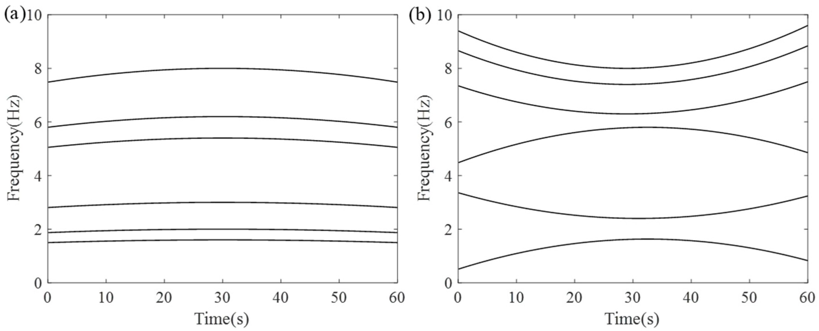
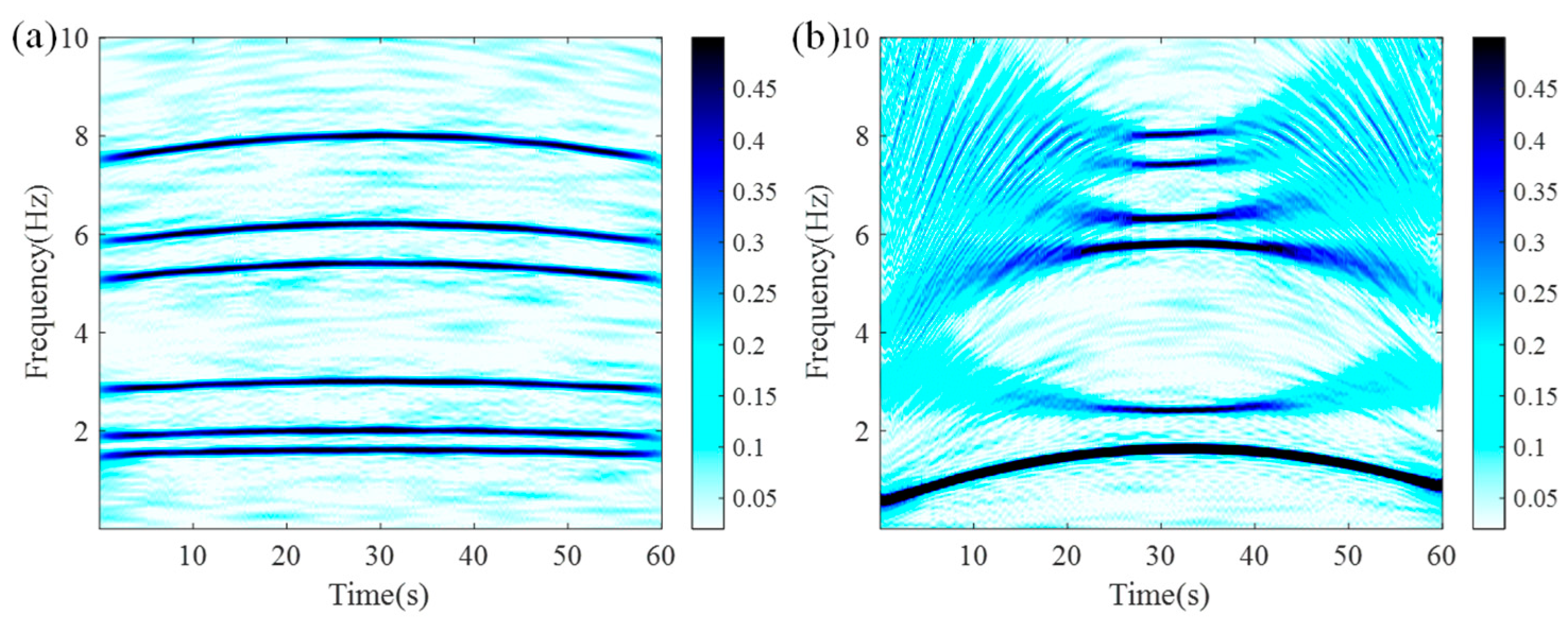
SBCT exhibits limited capability in analyzing non-stationary signals containing multiple fundamental frequency components that do not conform to a proportional relationship. As revealed by the mathematical formulation (e.g., Equation (8)), the core assumption of SBCT relies on the proportionality among IF trajectories. When the frequency components do not satisfy the proportional constraint, the matching capability of the method significantly degrades, as demonstrated by the example signals constructed earlier.

(2)

When non-stationary signals contain closely spaced IF components, the energy concentration capability of SBCT becomes insufficient. Specifically, when the frequency spacing between multiple IF components is small, the energy distribution obtained by SBCT tends to spread within the frequency support of the window function, resulting in blurred ridges and reduced resolution in the TFR, making it difficult to accurately distinguish adjacent components.

(3)

SBCT currently lacks a post-processing mechanism to enhance the energy concentration in the TFR. The time–frequency output of the existing SBCT algorithm is not subjected to energy reconstruction or optimization, which limits its potential for further improvement in energy concentration and time–frequency resolution. Introducing effective post-processing strategies, such as energy reassignment or enhancement operations, is anticipated to greatly enhance the readability and analytical accuracy of the TFR.

Therefore, it is imperative to design or improve TFA methods to address complex non-stationary signals containing non-proportional frequency components and closely spaced IF components. The method presented in this work specifically targets these challenges, focusing on resolving the challenges of SBCT when multiple fundamental components and closely spaced IFs coexist and enhancing the energy concentration and frequency resolution of the resulting TFRs.

3. Local Entropy Selection Scaling–Reassigning Chirplet Transform Method

This section mainly introduces the core mathematical theory of LESSRCT, which was developed based on SBCT and primarily includes the Rényi entropy-based TFR optimization criterion and the energy reconstruction-based concentration enhancement mechanism.

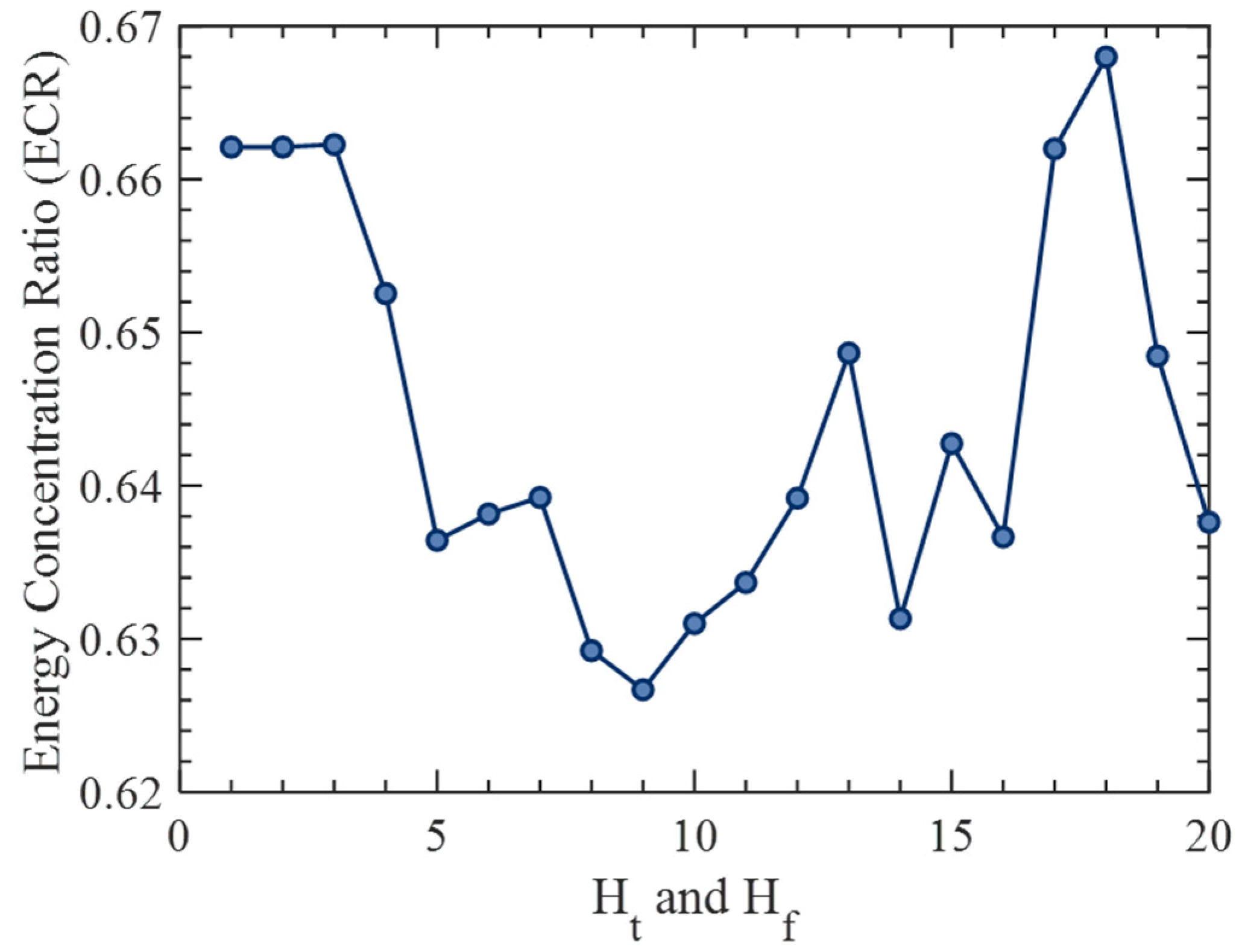
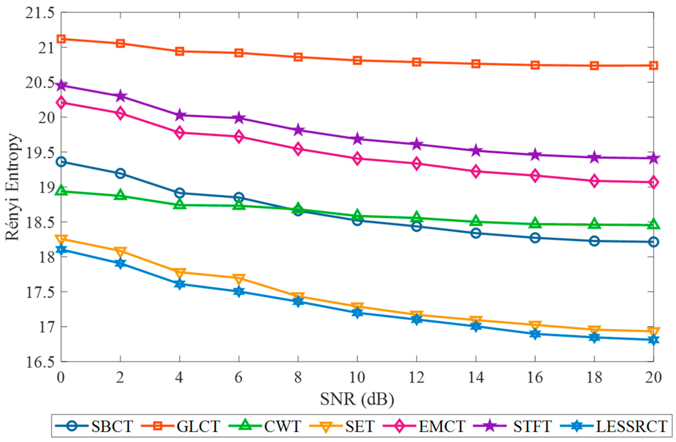
3.1. TFR Optimization Criterion Based on Rényi Entropy

The core idea of the TFR optimization criterion based on Rényi entropy is to divide the entire TFR into several local regions (i.e., time–frequency blocks). Within each block, Rényi entropy is employed to measure the energy concentration of the time–frequency distribution. By minimizing the local Rényi entropy, the CR is adaptively adjusted, enabling the most suitable time–frequency basis function to be chosen for each region. This approach effectively enhances the matching capability for multiple IF components in multi-component signals, thereby achieving more precise energy concentration in the TFR.

In this process, we first define a series of discrete CRs to approximate the signal’s modulation parameters. This discretization strategy not only allows for flexibility in adapting to the characteristics of different signals but also facilitates the optimization of the CR by continuously adjusting it, thereby maximizing the precision of the signal’s TFR. Specifically, the selection of discrete CRs is detailed as follows:

$$C=\tan (\theta )\cdot {\displaystyle \frac{F_S}{2T_S}}$$

(16)

In Equation (16), C represents the CR, θ is the rotation angle in the time–frequency plane, F_S denotes the sampling frequency, and T_S refers to the sampling time. This equation establishes the relationship between the rotation angle θ and C, where the modulation parameter C depends on the angle θ, the sampling frequency, and the sampling time.

$$\theta =-{\displaystyle \frac{\pi }{2}}+{\displaystyle \frac{\pi }{N_c+1}},\dots ,-{\displaystyle \frac{\pi }{2}}+{\displaystyle \frac{N_c\pi }{N_c+1}}$$

(17)

Equation (17) further describes the discrete nature of the CRs, with Nc indicating the number of discrete CRs. The angle θ is adjusted incrementally, dividing the TF plane into Nc + 1 sections, thus yielding N distinct discrete CRs.

To determine the optimal CR for windowed signals, we rely on the principle that the amplitude of CT reaches its maximum when the CR is consistent with the modulation ratio of the signal. This alignment ensures the best matching between the signal’s IF characteristics and the TFR. In this work, we propose using Rényi entropy as a quantitative measure to evaluate how well the CR matches the IF trajectory of the signal.

The theoretical foundation of this approach lies in the fact that when the CR matches the modulation ratio, the CT amplitude achieves its peak. Building on this, we select Rényi entropy as an appropriate criterion for assessing the CR-IF alignment, as it allows us to quantify the degree of match between the CR and the signal’s IF trajectory. By minimizing Rényi entropy, we can identify the optimal CR that best represents the signal in the time–frequency plane. The Rényi entropy of the TFR of order α can be described as:

$$H^{\alpha }={\displaystyle \frac{1}{1-\alpha }}{\log }_2\left({\displaystyle {\int }_{-\infty }^{+\infty }{\displaystyle {\int }_{-\infty }^{+\infty }{\left(\frac{\stackrel{⌢}{T}(t,\zeta )}{{\displaystyle {\int }_{-\infty }^{+\infty }{\displaystyle {\int }_{-\infty }^{+\infty }\stackrel{⌢}{T}(t,\zeta )dtd\zeta }}}\right)}^{\alpha }dtd\zeta }}\right)$$

(18)

where $\stackrel{⌢}{T}(t,\zeta )$ denotes the time–frequency distribution (TFD) function before normalization. It is a two-dimensional function with respect to time t and frequency ζ, representing the energy density of the signal at that point. In the context of Rényi entropy for TFR, an effective evaluation of the match between the CR and the IF can be achieved by performing integration throughout the time–frequency plane. To assess this alignment quantitatively, we apply the Rényi entropy formulation to the SBCT-based TFR. The entropy measure provides a criterion for selecting the optimal CR by minimizing signal dispersion and enhancing energy concentration. Based on the SBCT representation, Rényi entropy H^α is formulated as:

$$H^{\alpha }={\displaystyle \frac{1}{1-\alpha }}{\log }_2\cdot \left[{\displaystyle \iint \underset{n\to \infty }{\lim \sup }}{\left({\displaystyle \frac{\mathrm{SBCT}(f,t_c,a_1,a_2,\dots ,a_n)}{{\displaystyle \prod _{m=0}^{n+1}\mathrm{SBCT}}(f_m,t_m,a_1,a_2,\dots ,a_n)}}\right)}^{\alpha }dtdf\right]$$

(19)

The SBCT-based Rényi entropy formulation evaluates the alignment between the CR and the IF. Here, SBCT (f, t_c, a₁, a₂, …, a_n) represents the TFR.

$${\displaystyle \prod _{m=0}^{n+1}\mathrm{SBCT}}(f_m,t_m,a_1,a_2,\dots ,a_n)$$

(20)

Equation (20) denotes the product of SBCT values at different time–frequency points. The double integral spans the time–frequency plane, and α, typically set to 3, determines the entropy order. This formulation provides a quantitative criterion for CR selection by minimizing entropy to enhance energy concentration.

For multi-component signals, significant differences in modulation exist across both time and frequency domains. The challenge lies in approaches to reliably utilize Rényi entropy to allow the CR to adapt dynamically in both directions, ensuring it aligns with the varying characteristics of the signal. Notably, within a small time–frequency window, the signal can be approximated as having a linear modulation. Based on this assumption, we propose segmenting the entire time–frequency plane into multiple time–frequency blocks, within which Rényi entropy is individually computed. This approach enables localized entropy evaluation, ensuring that CR selection remains adaptive to variations in the signal. The TFR of SBCT, denoted as h(t, μ), is partitioned by moving a window function H(t, μ) along both the time and frequency directions, progressively covering the entire time–frequency plane. This segmentation provides a structured framework for computing Rényi entropy, refining the TFR, and enhancing the accuracy of TFA.

$$R(c,t,f)={\displaystyle \frac{1}{1-\alpha }}{\log }_2\cdot \left({\displaystyle {\int }_{-\infty }^{+\infty }{\displaystyle {\int }_{-\infty }^{+\infty }\frac{\left|h(c,\gamma ,\delta )H(\gamma -t,\delta -f)\right|}{{\displaystyle {\int }_{-\infty }^{+\infty }{\displaystyle {\int }_{-\infty }^{+\infty }\left|h(c,\gamma ,\delta )\right|H(\gamma -t,\delta -f)d\gamma d\delta }}}}}\right)d\gamma d\delta$$

(21)

$$M(t,f)=\left\{\begin{array}{l}1,-{\displaystyle \frac{\Delta t}{2}}<t<{\displaystyle \frac{\Delta t}{2}},-{\displaystyle \frac{\Delta f}{2}}<f<{\displaystyle \frac{\Delta f}{2}}\\ 0,otherwise\end{array}\right.$$

(22)

To enhance the flexibility of TFA, the TFR of a signal is divided into multiple smaller blocks, allowing for a more refined assessment of the match between the CR and the IF. The time and frequency intervals of each TF block are denoted as Δt and Δf, respectively. Additionally, the variable N_c is introduced to describe the time–frequency structure of the signal within a three-dimensional space h(c, t, f). Here, N_c represents the number of distinct CRs, while L × L/2 defines the frequency resolution, allowing the signal to be represented as a three-dimensional representation of size N_c × L × L/2.

Within this framework, different CRs applied to the SBCT method yield distinct TFR results. Assuming that the entire TFR is divided into H_t × H_f time–frequency blocks, each block corresponds to a localized time–frequency region. The Rényi entropy of each TF block is then computed to evaluate the degree of alignment between the CR and the IF trajectory within that region. Consequently, after entropy computation, the three-dimensional space h(c, t, f) is reduced in scale from N_c × L × L/2 to N_c × H_t × H_f, achieving a compressed representation of the signal’s overall structure.

Among these time–frequency blocks, each contains N_c entropy values. The block with the minimum entropy is considered the optimal time–frequency block, as it corresponds to the CR that best aligns with the time–frequency characteristics of that region. In other words, the chirp rate associated with this block most accurately captures the modulation features of the signal within the given time–frequency segment. By identifying the time–frequency block with the lowest entropy, the CR can be dynamically adjusted to adapt across the time–frequency plane, ultimately optimizing the overall TFR. This process can be mathematically described as follows:

$$\stackrel{⌢}{c}(t,f)=\underset{c}{\arg \min }\left\{R(c,t,f)\right\}$$

(23)

After computing the preliminary TFR, the Rényi entropy for each segment in the time–frequency plane is evaluated. By adjusting parameters, the entropy values for different time–frequency blocks at various chirp rates are compared. This process allows for the selection of the time–frequency blocks that exhibit the highest energy concentration. The corresponding time–frequency blocks are then combined to form an enhanced two-dimensional TFR with dimensions L × L/2. A key parameter in the Rényi entropy-based TFR optimization criterion is the size of the time–frequency block (H_t × H_f), which should be determined based on the local structural characteristics of the TFR generated by the scaled chirplet basis.

Through this approach, Rényi entropy is minimized, leading to a more focused and refined TFR. The final result is an entropy-enhanced SBCT (E-SBCT), which offers a more accurate and concentrated representation of the signal in the time–frequency domain.

Compared with other sparsity and concentration measures, such as Shannon entropy, L1-norm, the Gini index, or spectral kurtosis, Rényi entropy offers greater flexibility and adaptability due to its adjustable order parameter α. Specifically, when α > 1, Rényi entropy places more emphasis on high-energy components, making it particularly sensitive to localized concentrations in the TFR. This property is essential for distinguishing closely spaced IF components and enhancing energy aggregation in multi-component signals. Moreover, Rényi entropy has been widely adopted in state-of-the-art TFA frameworks, such as EMCT and SET, where time–frequency resolution and component separability are critical. In contrast, Shannon entropy tends to be less sensitive to sharp energy peaks, and L1-norm lacks a probabilistic interpretation. Therefore, the use of Rényi entropy in this study ensures both theoretical rigor and empirical effectiveness in evaluating and enhancing the concentration of TFRs.

3.2. Energy Reconstruction-Based Concentration Enhancement Mechanism

To deeply analyze the working principle of LESSRCT, we will begin by investigating the TFR of non-stationary signals obtained via STFT, further exploring its role in enhancing energy display.

$$\left\{\begin{array}{l}F(t,f)={\displaystyle {\int }_{-\infty }^{\infty }s(u)\cdot \mathrm{g}(u-t)\cdot e^{-j\omega (u-t)}du}\\ s(t)=A(t)\cdot e^{j\theta (t)}\end{array}\right.$$

(24)

where we define F(t, f) as the TFD of STFT, where the signal s(t) represents a time-varying signal. A(t) denotes the amplitude modulation, and θ(t) represents the phase component that changes with time at each instant. g(u − t) is the window function, used for localizing the signal. According to Parseval’s theorem, we can further expand and re-express STFT in Equation (18):

$$F(t,f)=\left(1/2\pi \right){\displaystyle {\int }_{-\infty }^{\infty }\stackrel{⌢}{s}(\tau )\cdot \stackrel{⌢}{g}(f-\tau )}\cdot e^{j\xi t}d\tau$$

(25)

In this case, the integrand functions are represented as the Fourier transforms (FTs) of g(·) and s(·). To facilitate understanding and analysis, we will focus on harmonic signals with a constant amplitude A and frequency f for further investigation. The STFT of such a harmonic signal can be stated as:

$$F(t,f)=A\cdot \stackrel{⌢}{g}(f-f_0)\cdot e^{j{\omega }_{0}t}$$

(26)

The TFD of SBCT, as described in Section 2.1, is defined as follows:

$$SBCT\left(f_c,u,t_c\right)={\displaystyle {\int }_{-\infty }^{+\infty }s\left(u\right){\omega }_{\sigma }\left(u-t_c\right)e^{-j\omega (u-t)}du}$$

(27)

Based on the Rényi entropy-based TFR optimization criterion derived in Section 3.1, we propose E-SBCT. Accordingly, Equation (26) can be further expressed as:

$$E-SBC{T}_s\left(t,f\right)=A\cdot \stackrel{⌢}{g}(f-{\stackrel{⌢}{f}}_0)\cdot e^{j{\stackrel{⌢}{f}}_{0}t}$$

(28)

To significantly enhance the quality of the TFR, an advanced one-dimensional IF estimation method is employed. Based on this, we introduce the frequency reassignment operator (RO), as shown below. This approach not only optimizes the frequency reassignment process but also further improves signal energy aggregation in the time–frequency domain, thus providing strong support for more precise signal analysis.

$$f_r(t,f)=\left\{\begin{array}{l}\underset{f}{\arg \max }\left|E-SBC{T}_s\left(t,f\right)\right|,if\left|E-SBC{T}_s\left(t,f\right)\right|\ne 0\\ 0,if\left|E-SBC{T}_s\left(t,f\right)\right|=0\end{array}\right.$$

(29)

Due to the symmetry of the Gaussian window function, its Fourier transform (FT) reaches a peak at zero frequency. Therefore, the RO can be further optimized and rewritten. This representation leverages the unique properties of the Gaussian window function, making the frequency reassignment process more accurate and effectively enhancing signal energy aggregation in the time–frequency domain.

$$f_r(t,f)=\left\{\begin{array}{l}{f}_j(t),iff\in \left[f_j(t)-\Delta ,f_j(t)+\Delta \right]\\ 0,\mathrm{otherwise}\end{array}\right.$$

(30)

Therefore, the RO can be further expressed as:

$$RO(t,f)=\delta (f-f_r(t,f))=\left\{\begin{array}{c}1,\left|f-f_r(t,f)\right|<\epsilon \\ 0,\mathrm{otherwise}\end{array}\right.$$

(31)

In this process, δ (·) represents the Dirac delta function. In practical applications, precisely aligning the RO with the frequency center is a complex and challenging task. To overcome this difficulty and achieve a close approximation, we introduce a small parameter ε to relax the constraints appropriately.

In the energy reallocation-based concentration enhancement mechanism, the parameter ε plays a crucial role in regulating the redistribution behavior of time–frequency energy. Its selection has a substantial influence on the clarity and concentration of the resulting TFR. Specifically, a smaller ε is more suitable for signals with closely spaced frequency components and high demands on time–frequency resolution, as it helps suppress energy diffusion and enhances the representation of dominant components. Conversely, for signals with rapidly varying frequencies or more dispersed components, a larger ε allows broader frequency participation in the reconstruction process, thereby improving the robustness and adaptability of the representation. Based on extensive empirical evaluations across various signal types, setting ε = 0.4 generally offers a good trade-off between energy concentration and global fidelity, making it a reliable and versatile choice.

Based on the above derivation and analysis, an efficient TFA method, termed LESSRCT, is proposed to enhance energy concentration and readability of the TFR, thereby improving the interpretability of complex signals.

$$LESSRCT(t,f)=E-SBCT(t,f)\cdot RO(t,f)$$

(32)

3.3. Implementation of the LESSRCT Method

Based on the theoretical derivations and discussions presented in Section 3.1 and Section 3.2, the implementation procedure of the LESSRCT algorithm is outlined in the form of pseudocode in Algorithm 1. The algorithm was developed and executed using MATLAB R2024b, ensuring numerical stability and reproducibility in practical applications.

Algorithm 1: LESSRCT algorithm

Step 1: Initial Parameter Configuration (1) The signal s(t), the length of the window L, the sampling frequency Fs, and the count of Gaussian windows K, along with the values of delta and ε. (2) local-TFR ← zeros(NH, NL). Step 2: Computation of the local-TFR   for i = 1: NH   for j = 1: NH     local-TFR(i, k) ← SBCT(t, f).     local-TFRg(i, k) ← SBCTg′(t, f).   end for   end for Step 3: Localized Entropy Selection (3) Apply entropy to divide the local time–frequency segments.    for i = 1: N     E-SBCT(:, :) ← the minimum value (entropy (local-TFR (:, i)))     E-SBCT (g)’(:, :) ← the minimum value (entropy (local-TFRg(:, i)))    end for Step 4: Energy Reconstruction (4) Compute:E ← mean(s(t)).   for i = 1: NL      for j = 1: NL        LESSRCT (i, j) ← LESSRCT (i, j) + sub-TFR (i, j)       if abs(i-fr(i, j)) < ε        δs(i, j) = 1       end for      end for   end if (5) LESSRCT(i, j) ← E-SBCT(i, j)·δs(i, j).

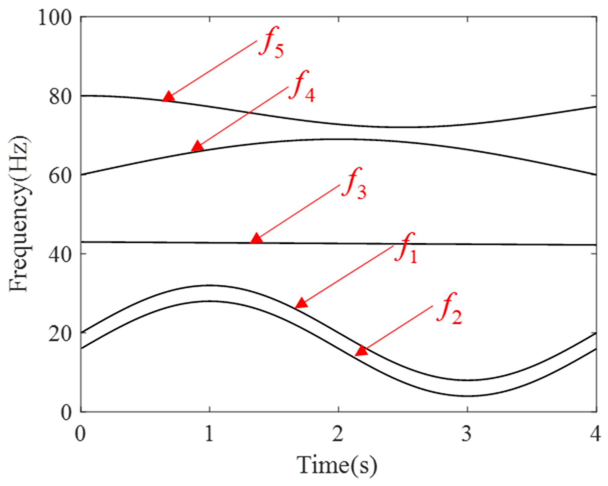
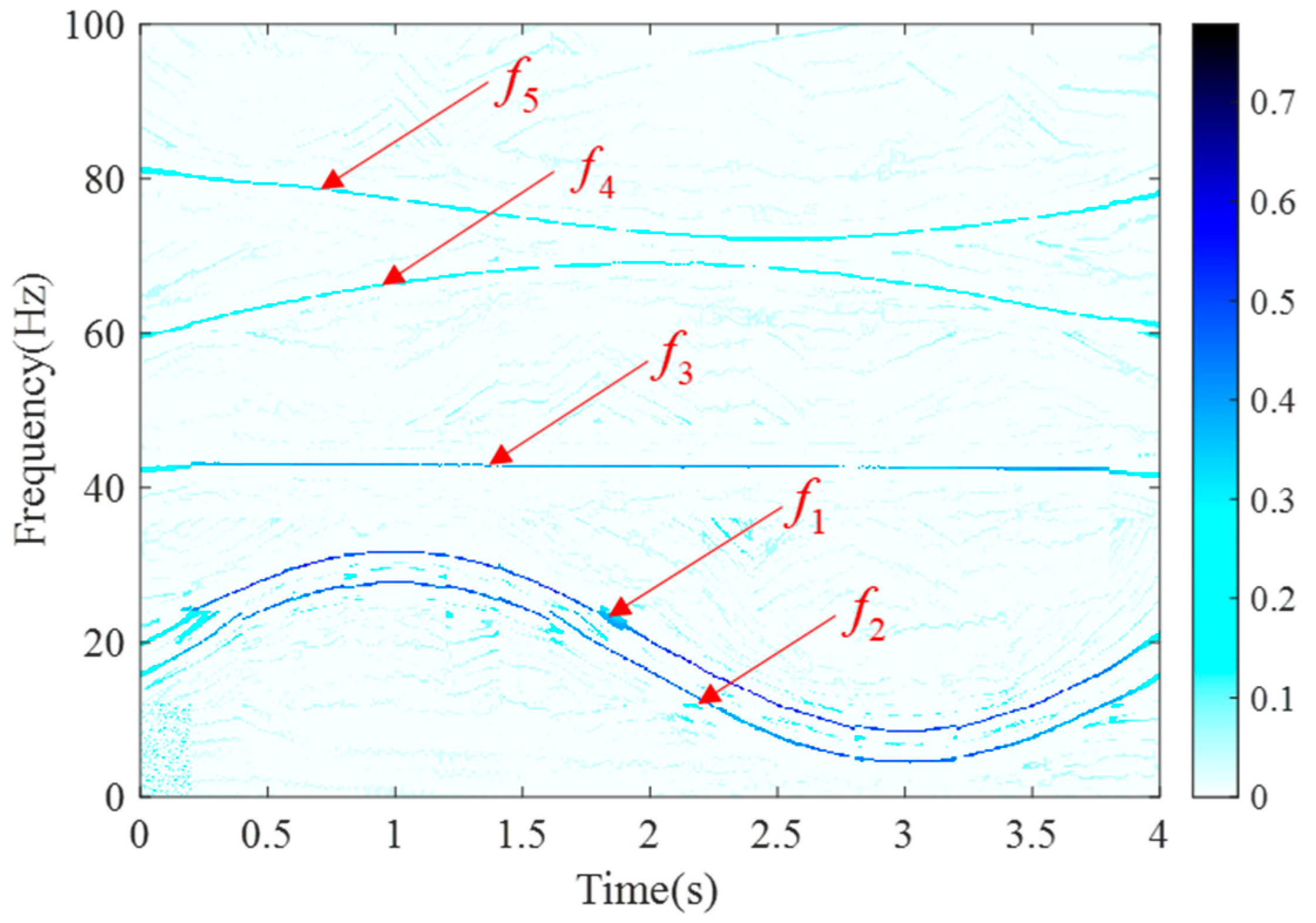
4. Numerical Experimentation

To evaluate the performance and effectiveness of LESSRCT in analyzing signals characterized by non-proportional features and closely spaced instantaneous frequency components, a set of simulated experimental signals was constructed in this study and compared with other TFA methods. The comparison focused on key metrics, such as energy concentration, time, and frequency accuracy, providing a comprehensive demonstration of the advantages of the LESSRCT method in TFA. The signal set used in the experiments was complex and exhibited strong disproportionate characteristics, with the specific signals formulated as:

$$s_1(t)={\displaystyle {\sum }_{K=1}^5\sin (2\pi \cdot F_K(t))}\cdot A_K(t)+noise(t)$$

(33)

where Ak(t) represents the time-varying amplitude (envelope) of the k-th component, while F_K(t) = ∫f_K(t) dt denotes the instantaneous phase derived from the IF f_k(t). This construction enables the simulation of multiple non-proportional components with varying energy levels and frequency behaviors. To more accurately emulate real-world conditions, additive white Gaussian noise with a signal-to-noise ratio (SNR) of 10 dB was incorporated into the synthetic signal. This process aimed to replicate the typical noise characteristics encountered in practical environments. The IF components of each signal element were defined as follows:

$$\left\{\begin{array}{l}{f}_1(t)=19+12\sin (0.5\pi t)\\ f_2(t)=16+12\sin (0.5\pi t)\\ f_3(t)={\displaystyle \frac{1}{350}}{\left(t-29\right)}^2+41\\ f_4(t)=60+9\sin (0.25\pi t)\\ f_5(t)=76+4\cos (0.4\pi t)\end{array}\right.$$

(34)

The amplitudes of the individual signal components A_i(t) (i = 1~5) were set to constant values of 1.1, 1.0, 0.85, 0.65, and 0.6, respectively, in order to construct signal components with varying energy levels and pronounced disproportionate characteristics. The simulated signal was sampled at a frequency of 200 Hz, with a total analysis duration of 4 s. Based on the previously defined IFs f_k(t) and their corresponding amplitudes A_k(t), the phase functions were obtained via integration as F_K(t) = ∫f_K(t) dt, which were then used to synthesize the composite signal s₁(t). Figure 3 presents the ideal TFD of the signal s₁(t), clearly illustrating its temporal evolution, the variation trends in its IF components, and the corresponding energy distribution characteristics.

The artificially constructed signal s₁(t) was analyzed using the LESSRCT method, and the resulting TFD is shown in Figure 4. The method successfully captured all IF components, and, notably, it was able to accurately separate and clearly identify closely spaced components, such as f₁(t) and f₂(t). The generated TFD exhibits high time–frequency resolution and strong energy concentration. These results fully validate the accuracy and robustness of LESSRCT in analyzing complex, multi-component non-stationary signals, demonstrating its significant advantages in constructing high-precision TFRs.

To thoroughly assess LESSRCT’s effectiveness, a comparative study was performed against several conventional and widely used TFA methods, including SBCT, GLCT, CWT, SET, EMCT, and STFT. To guarantee an unbiased comparison, all methods employed identical parameter settings. The resulting TFDs are illustrated in Figure 5a–f. As shown, none of the six TFA methods succeeded in accurately resolving all five IF components, with particularly poor performance in distinguishing the closely spaced components f₁(t) and f₂(t). The generated TFDs exhibited varying degrees of energy smearing and spectral blurring, revealing significant limitations in capturing the detailed time–frequency structure of the signal.

To comprehensively, accurately, and objectively assess the effectiveness of the introduced LESSRCT method in analyzing the non-stationary signal s₁(t), we introduced two representative quantitative evaluation metrics: Rényi entropy and the Structural Similarity Index Measure (SSIM). These metrics were also used to compare LESSRCT with six mainstream TFA methods.

The first metric, Rényi entropy, is a widely used information-theoretic measure that quantifies the energy concentration of a TFR. For a two-dimensional normalized TFR P(t,f), the Rényi entropy of order α is defined as:

$$H_{\alpha }(P)={\displaystyle \frac{1}{1-\alpha }}{\log }_2\left({\displaystyle \sum _{t,f}P}{(t,f)}^{\alpha }\right)$$

(35)

where P(t,f) denotes the normalized energy distribution at time t and frequency f, and α is the Rényi order, typically set to α = 2. A lower Rényi entropy value signifies greater energy concentration within the TFR, reflecting a better ability to localize signal components and reveal fine time–frequency structures.

The second metric, the SSIM, assesses the structural similarity between two images and is particularly effective in evaluating the visual consistency between the ideal TFR and those generated by different TFA methods. It is defined as:

$$\mathrm{SSIM}(x,y)={\displaystyle \frac{(2{\mu }_x{\mu }_y+C_1)(2{\sigma }_{xy}+C_2)}{({\mu }_x^2+{\mu }_y^2+C_1)({\sigma }_x^2+{\sigma }_y^2+C_2)}}$$

(36)

where x and y represent the ideal TFR and the generated TFR, respectively; μ_x and μ_y are the means; σ_x² and σ_y² are the variances; and σ_xy is the covariance between x and y. The constants C₁ = (K₁L)² and C₂ = (K₂L)² are included to stabilize the division, with L denoting the dynamic range of the pixel values; typically, K₁ = 0.01 and K₂ = 0.03. The SSIM measures structural similarity, with values closer to 1 indicating better similarity.

By combining these two metrics, we aimed to objectively evaluate the performance of each method from the perspectives of both energy concentration and structural fidelity. The Rényi entropy results for each method applied to s₁(t) are summarized in

Table 1. Quantitative comparison of Rényi entropy values for different TFA methods.

Method	SBCT	GLCT	CWT	SET	EMCT	STFT	LESSRCT
Rényi entropy	16.0713	18.3627	16.8712	14.7565	16.8717	16.9143	13.5316

, providing a quantitative measure of energy localization. The corresponding SSIM comparison results are visually illustrated in Figure 6, further demonstrating the structural similarity between each method’s output and the ideal TFR.

According to the results presented in Table 1, compared with other commonly used TFA methods, the LESSRCT method achieves a minimum Rényi entropy value of 13.5316. This indicates that the TFR generated by LESSRCT exhibits a high degree of energy concentration, demonstrating superior energy aggregation performance and a clearer time–frequency structure, which is beneficial for highlighting the intrinsic characteristics of the signal. In contrast, the GLCT method yields the highest Rényi entropy value of 18.3627, suggesting that its TFR energy distribution is more dispersed, resulting in a blurred time–frequency structure that struggles to effectively capture the local details of the signal.

Meanwhile, as shown in the SSIM comparison in Figure 6, the LESSRCT method attains the highest structural similarity index, further validating the strong consistency between its output and the ideal TFR. In other words, LESSRCT is capable of more accurately reconstructing the time–frequency features of the signal, closely approximating the structural details and overall pattern of the ideal representation.

In summary, based on multiple experimental validations, the proposed LESSRCT algorithm demonstrates excellent performance on the constructed s₁(t) signal. Despite the presence of non-proportional fundamental frequency components and closely spaced signal components, LESSRCT effectively performs precise TFA and energy concentration, exhibiting strong anti-interference and resolution capabilities. This highlights its practical value and potential application prospects in complex signal processing scenarios.

5. Validation in Practice

This section comprehensively evaluates the efficiency of the LESSRCT method using three real experimental signals. The first dataset consists of echolocation signals from bats, the second contains vibration signals from a faulty bearing, and the third is vibration data collected from the planetary gearbox of a wind turbine. These datasets represent complex signal types from different domains, providing strong support for verifying the universality and robustness of the LESSRCT method.

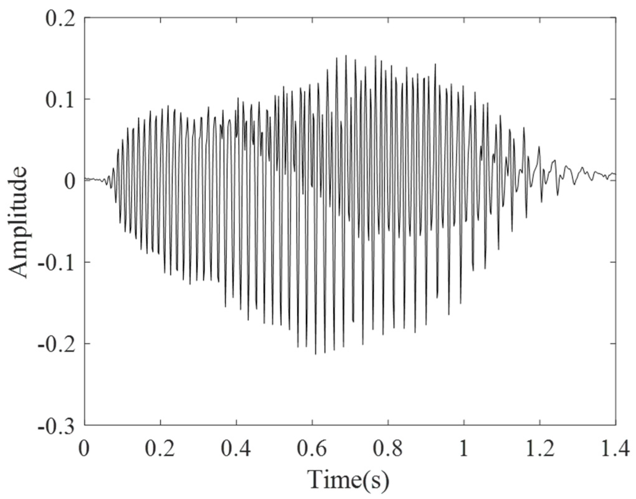
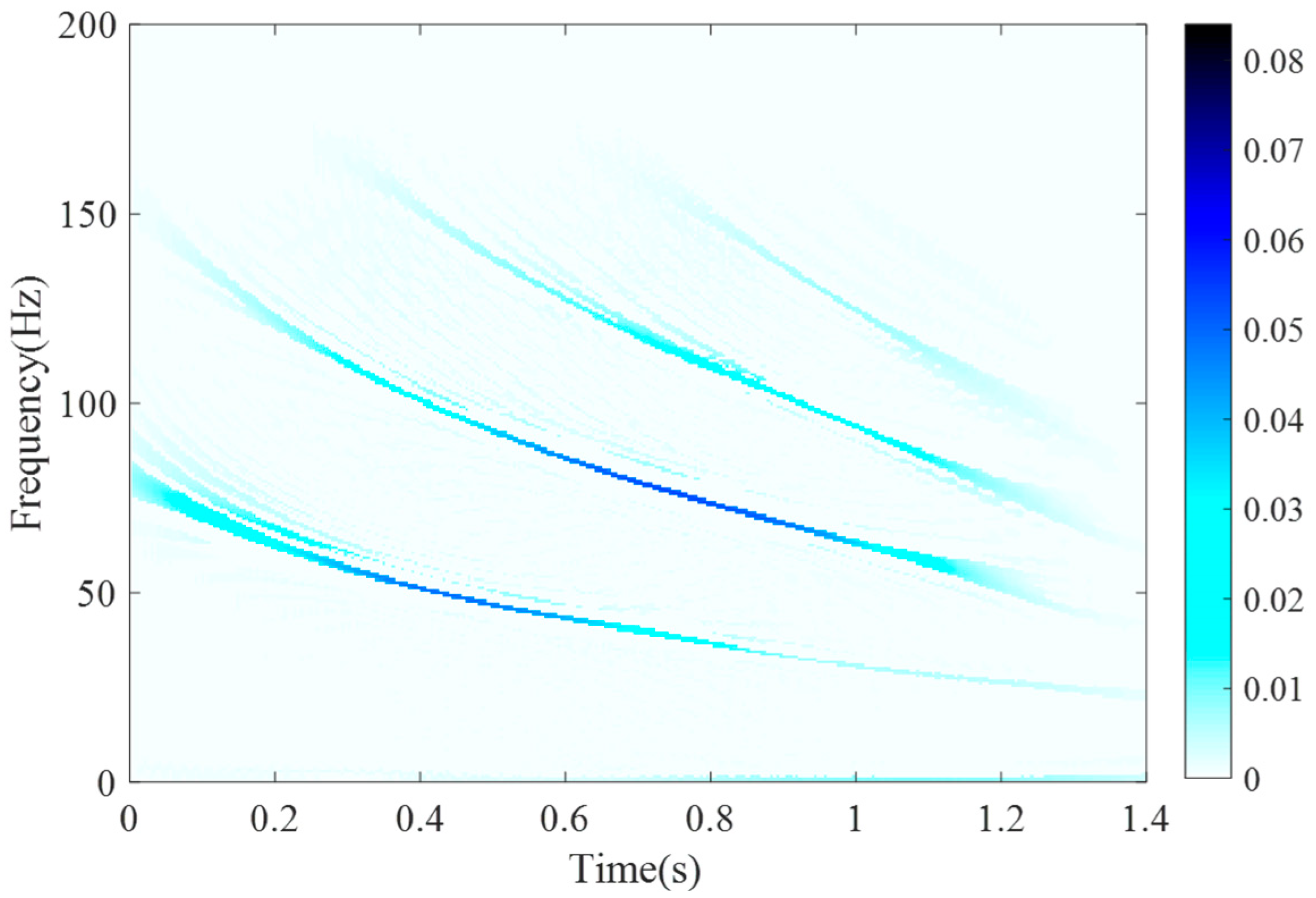
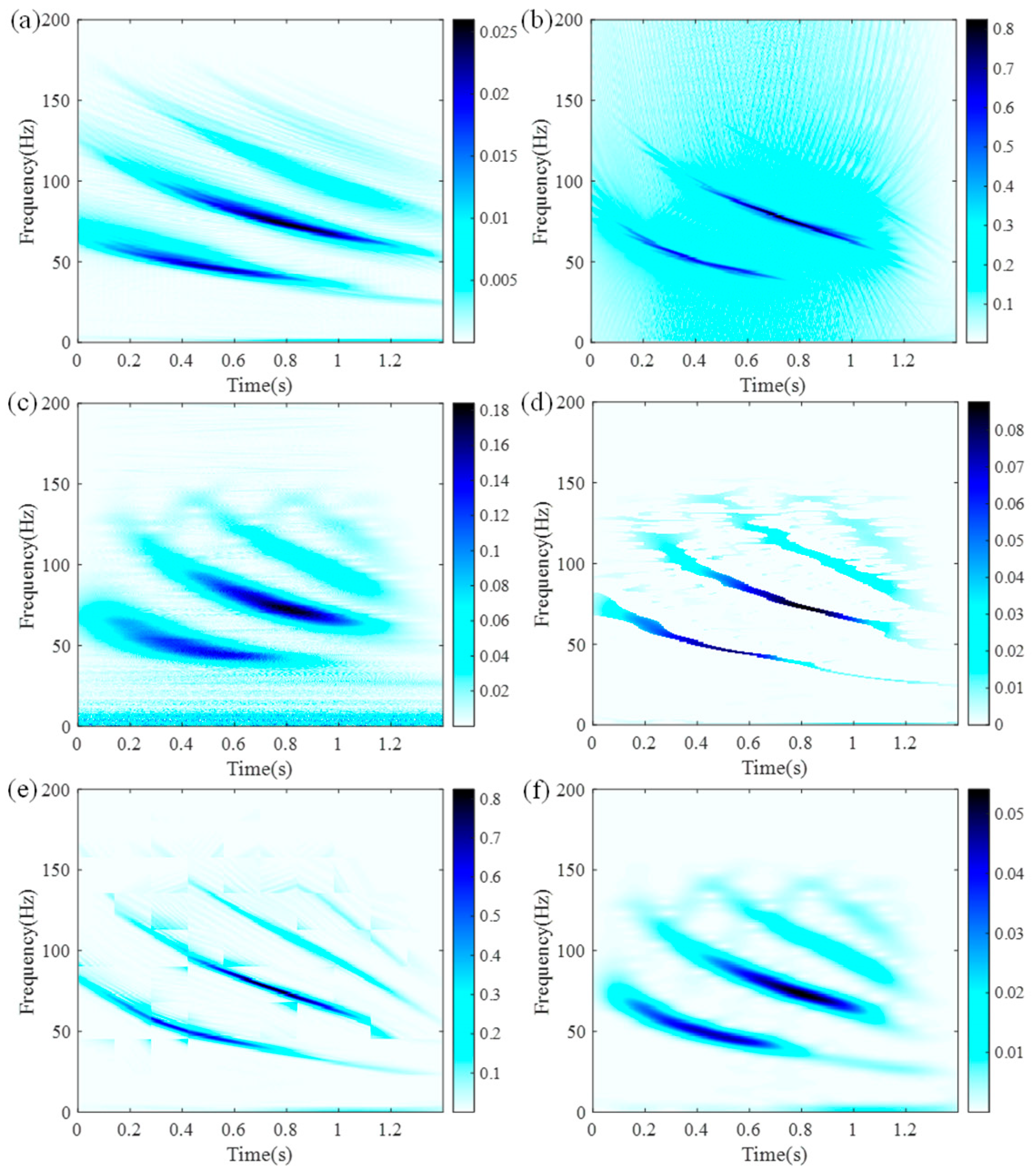
5.1. Evaluation of Bat Echolocation Calls

In this set of experiments, we conducted a systematic analysis of echolocation signals emitted by bats. These signals consist of a series of short, high-frequency ultrasonic pulses that bats use for spatial perception and target localization. A prominent characteristic of such signals is their non-proportional IF components. The signals were recorded at a sampling frequency of 450 Hz with a total duration of 1.4 s. The time-domain waveform of the captured signal is illustrated in Figure 7.

To validate the functionality of the proposed LESSRCT method in processing such biologically complex signals, we compared its TFR with those generated by several widely used TFA techniques, including SBCT, GLCT, CWT, SET, EMCT, and STFT. For consistency, all methods were applied using an identical window length of 200. The TFR produced by LESSRCT is shown in Figure 8. As observed, LESSRCT demonstrates outstanding capability in identifying all frequency components while effectively concentrating energy in the time–frequency domain, yielding a highly focused and structurally coherent representation.

In contrast, the other TFA methods exhibit notable limitations, as shown in Figure 9a–f. Both STFT and CWT result in significant energy diffusion and structural distortion, rendering them ineffective in capturing subtle frequency variations. The SET method struggles to distinguish closely spaced components, leading to limited resolution. Although EMCT is capable of detecting frequency trajectories to some extent, its results suffer from discontinuity, resulting in instability. The TFR produced by SBCT shows low energy concentration, leading to a blurred representation. Moreover, GLCT introduces noticeable cross-components, which obscure the true frequency information and compromise the interpretability and accuracy of the analysis.

To objectively assess the degree of energy concentration performance of various TFA methods, the Rényi entropy values of the TFRs obtained by each method were calculated, as shown in Figure 10. The proposed LESSRCT method yielded the lowest Rényi entropy value (11.5293), indicating the most concentrated energy distribution in the time–frequency domain and superior focusing capability. In contrast, methods such as GLCT and CWT exhibited significantly higher Rényi entropy values, reflecting a pronounced energy diffusion in their TFRs, which led to blurred representations and compromised both the accuracy and stability of the analysis.

The above analysis demonstrates that the LESSRCT method exhibits a significant advantage in time–frequency concentration compared to the six other mainstream TFA methods. The size of the time–frequency block H_t × H_f is a crucial parameter in the LESSRCT method, and the density of these blocks affects the analysis performance to some extent. However, it is noteworthy that increasing the number of time–frequency blocks does not necessarily lead to better analysis results. On the contrary, the optimal TFA performance is often achieved with a moderate block size. To objectively quantify the degree of energy concentration in the TFRs computed with different block sizes, the Energy Concentration Ratio (ECR) is introduced, defined as follows:

$$ECR={\displaystyle \frac{{\displaystyle {\sum }_{t=t_1}^{t_2}{\displaystyle {\sum }_{f=f_1}^{f_2}{\left|TFR\left(t,f\right)\right|}^2}}}{{\displaystyle {\sum }_{t=1}^T{\displaystyle {\sum }_{f=1}^F{\left|TFR\left(t,f\right)\right|}^2}}}}$$

(37)

where TFR(t, f) denotes the energy value of the TFR at time index t and frequency index f, [t₁, t₂] and [f₁, f₂] represent the time and frequency intervals of interest, and T and F are the total number of time and frequency points in the TFR, respectively. The ECR quantifies the proportion of energy within the region of interest relative to the total energy of the time–frequency plane; values closer to 1 indicate higher energy concentration.

In this study, the size of the time–frequency blocks was varied from 1 × 1 to 20 × 20, with ECR values calculated at each increment. The energy-focused region was set within the time interval of 0.4 to 1.0 s and the frequency interval of 50 to 150 Hz. As shown in Figure 11, the ECR reaches a relatively high value at 4 × 4 in the lower block size region and attains its maximum at 18 × 18 in the higher block size region. However, increasing the block size excessively leads to a rectangular effect in the TFRs, causing blurring and reduced time–frequency resolution. Therefore, considering both time–frequency resolution and energy concentration, a block size of 4 × 4 was chosen in this work. It is worth noting that all quantitative analyses of TFRs in this study were conducted based on this block size.

5.2. Inner Race Defect Testing in Rolling Bearings

Further experiments were conducted as a second stage using the Mechanical Fault Simulator Mechanical Fault Simulator (MFS-PK5M, SpectraQuest Inc., Richmond, VA, USA) to simulate inner race defects in rolling bearings. The experimental setup is shown in Figure 12, where the shaft is driven by an electric motor, and its speed is precisely controlled by an AC drive. The shaft is supported by two ball bearings. Detailed information about the faulty bearing is provided in

Table 2. Specifications for the bearings employed in the inner race fault test.

Fault Type	Pitch Diameter	Number of Balls	Ball Diameter	FCF
inner race fault	38.52 mm	9	7.94 mm	5.43 fr

. It is noteworthy that f_r represents the bearing’s rotational frequency. During the experiment, vibration signals were captured using an ICP accelerometer (PCB Piezotronics Inc., Depew, NY, USA) with a sampling rate of 200 kHz. The shaft speed varied between 13 Hz and 27.8 Hz throughout the test. This experimental design allowed for a comprehensive analysis of the fault signal characteristics at different rotational speeds.

To effectively analyze the non-stationary vibration signals of faulty bearings, the original signal was first downsampled to 600 Hz, with a total duration of 4 s. Figure 13 presents the time-varying rotational speed profile of the bearing under the given operating condition, highlighting significant non-stationary characteristics during operation. The LESSRCT method was then employed as the primary approach for TFA, where the window length was set to 450 in order to more effectively reflect the signal’s localized time-domain characteristics. The corresponding TFR is shown in Figure 14.

To comprehensively evaluate the performance of the LESSRCT method in time–frequency resolution and energy concentration, its results were compared against six widely used TFA methods, namely, STFT, CWT, SET, GLCT, SBCT, and EMCT. All methods were tested under consistent parameter settings and processing conditions to ensure the fairness and reproducibility of the comparison.

As illustrated in Figure 14, the LESSRCT method successfully captures the bearing fault characteristic frequencies (FCFs) and their corresponding harmonic frequencies, such as fr, 2 fr, 3 fr, 10 fr, 11 fr, and 12 fr, with well-defined time–frequency energy concentration, demonstrating exceptional time–frequency readability. In contrast, other TFA methods, including GLCT, CWT, and STFT, fail to accurately extract all frequency components, exhibiting noticeable blurring effects, as shown in Figure 15b,c,f. The SET method reveals discontinuous IF trajectories and suffers from energy leakage, as depicted in Figure 15d. Although the TFRs obtained using SBCT and EMCT can capture the FCF and most high-frequency components, such as 11 fr and 12 fr, they still struggle to accurately identify the low-frequency components, resulting in some blurring effects, as demonstrated in Figure 15a,e.

To further quantitatively assess the energy concentration capability of the various TFA methods, the Rényi entropy values of the TFRs generated by each method were calculated, as summarized in

Table 3. Comparison of Rényi entropy values for TFRs generated by different TFA methods.

Method	SBCT	GLCT	CWT	SET	EMCT	STFT	LESSRCT
Rényi entropy	18.1515	20.7281	18.4348	15.1607	19.0051	19.3523	16.6139

. As a key metric reflecting the energy distribution characteristics of a TFR, a lower Rényi entropy indicates a higher degree of energy concentration in the time–frequency domain. The results show that the proposed LESSRCT method achieves the lowest Rényi entropy value (16.7139), suggesting superior ability in concentrating signal energy and providing a more compact and interpretable TFR. In contrast, traditional methods, such as GLCT, EMCT, and STFT, yield significantly higher entropy values, indicating more dispersed energy distributions and limited capability in capturing the instantaneous features and localized structures of non-stationary signals.

In TFA, noise acts as a central element that affects the performance of various methods. The robustness of a technique against noise is an important indicator of its practical applicability. To objectively assess the noise resistance of different TFA approaches, we computed the Rényi entropy values of the TFRs generated by the proposed LESSRCT method and the six other representative techniques under SNRs ranging from 0 dB to 20 dB, with an increment of 2 dB. The results are illustrated in Figure 16.

As demonstrated in the figure, the Rényi entropy of the LESSRCT method consistently remains the lowest across all SNR levels, indicating its superior energy concentration and strong robustness to noise. The SET method also achieves relatively low entropy values under certain SNR conditions. However, it is worth highlighting that SET extracts the time–frequency ridge energy based on thresholding, which, while leading to numerically concentrated energy, often fails to capture the actual structural features of the signal, as reflected in Figure 15d. In contrast, the other methods (including STFT, CWT, GLCT, SBCT, and EMCT) generally yield higher entropy values under varying noise levels, suggesting that their TFRs tend to be more energy-dispersive when subjected to noise interference.

In summary, the evaluation of the faulty bearing signal demonstrates that the LESSRCT method effectively captures complex time–frequency features and maintains high resolution even in the presence of strong noise and closely spaced frequency components. The comparative analysis further confirms the superiority of LESSRCT in dealing with challenging nonlinear, non-stationary, and non-proportional signals.

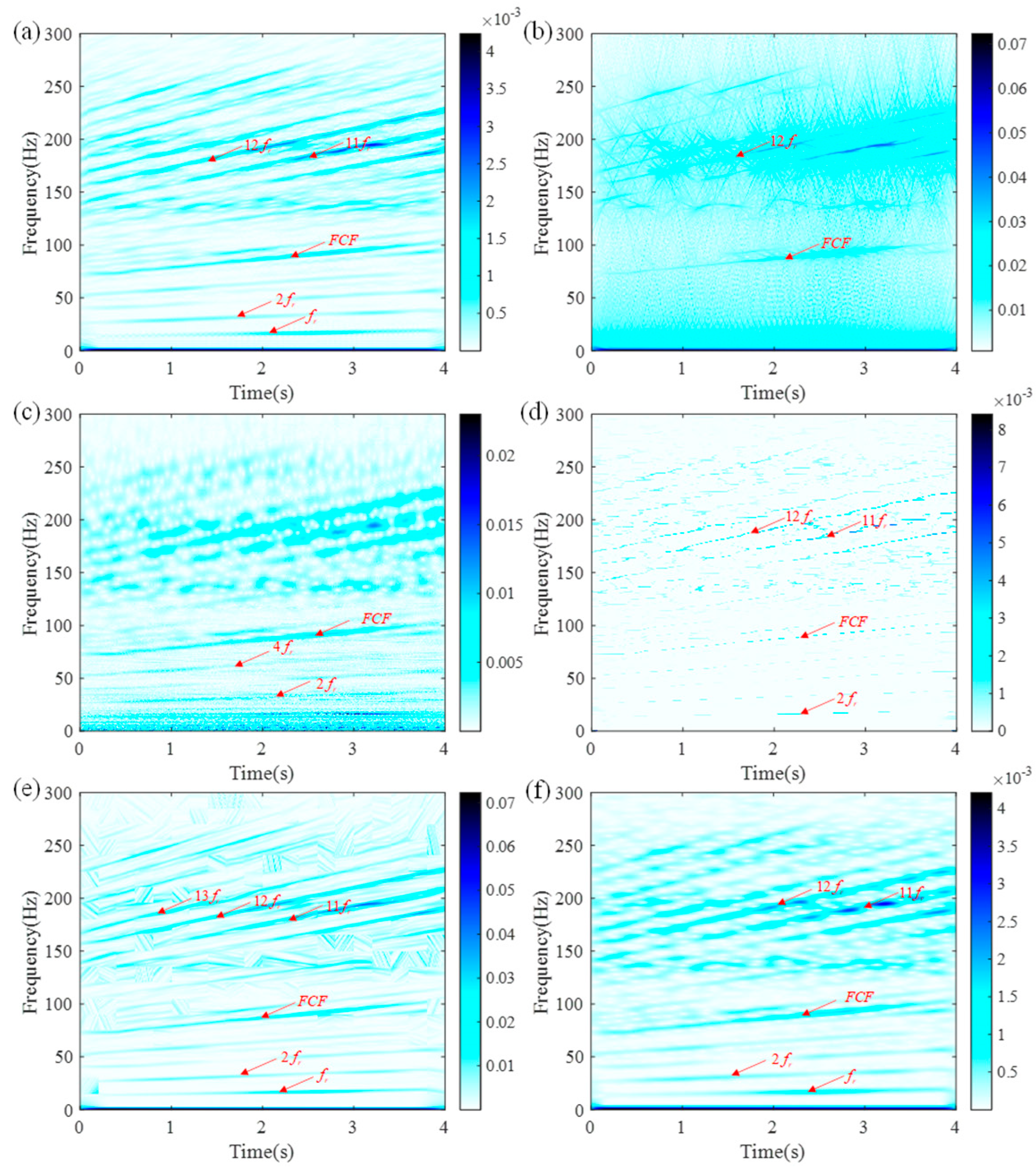
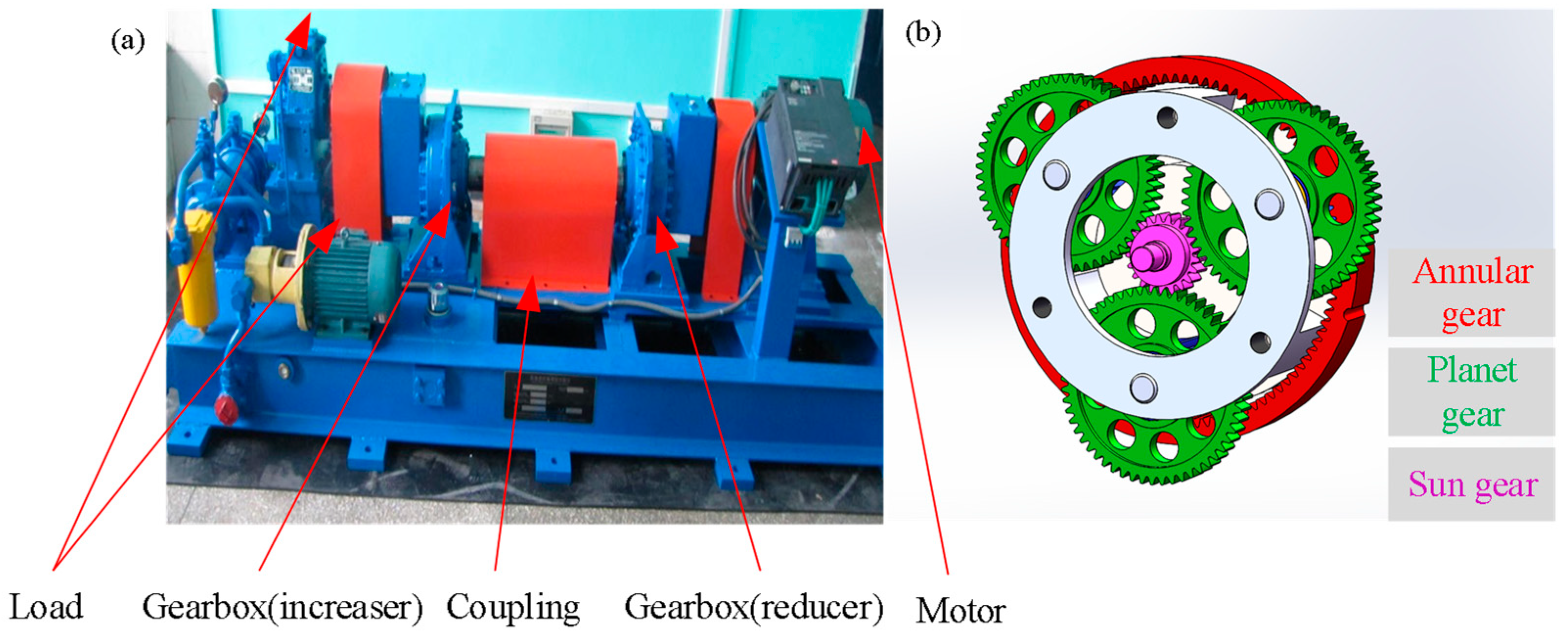
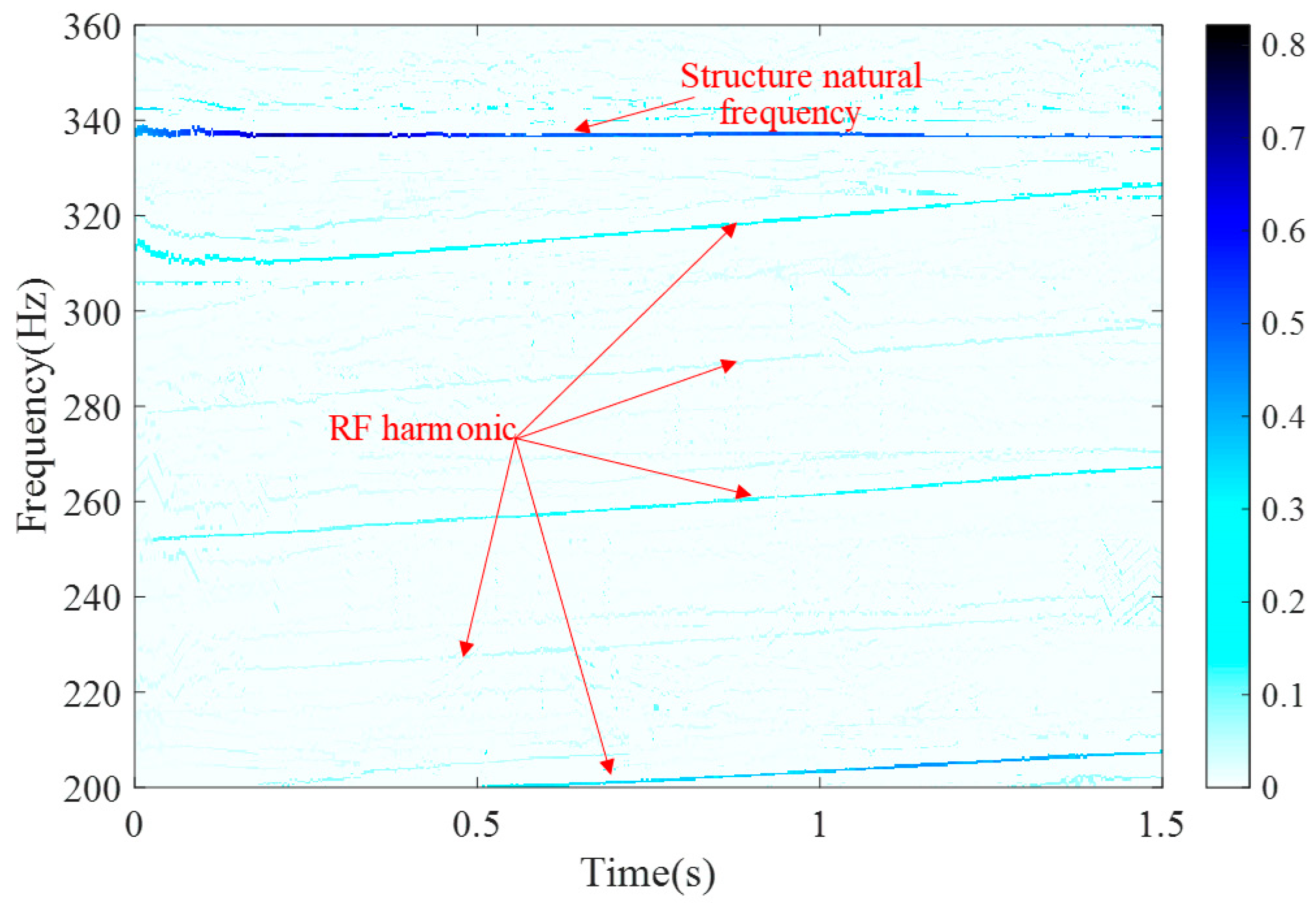
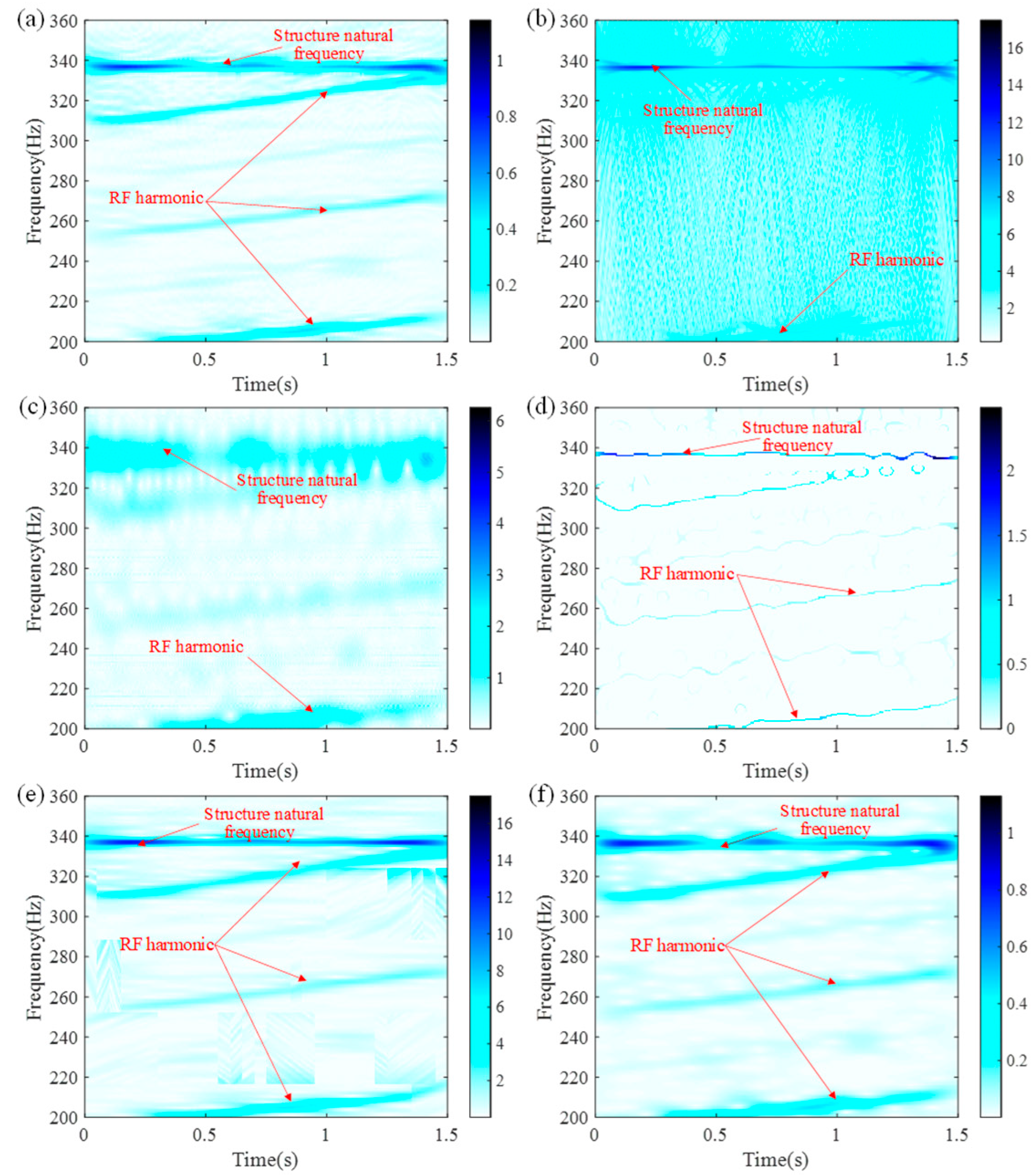
5.3. Evaluation of Gearbox Performance in Wind Turbine Power Transmission

The third experimental signal was obtained from a scaled-down wind turbine test platform designed to simulate the dynamic behavior of gearbox systems under realistic conditions. The comprehensive design of the test rig, the experimental setup, and the configuration of the planetary gear system are illustrated in Figure 17a,b. The platform is equipped with two identical gearboxes, both employing a compound gear system design [20] to enhance load transmission and adaptability. To more accurately replicate real-world operating conditions, a high-pressure hydraulic system is used to apply adjustable loads to the drivetrain via the driving motor. For vibration data acquisition, an accelerometer (Model 3056B1, PCB Piezotronics Inc., Depew, NY, USA) was precisely mounted on the top of the accelerated gearbox, ensuring high-precision and real-time monitoring of the gearbox vibration response throughout the experiment.

During the signal analysis, the original dataset was first downsampled to a sampling rate of 720 Hz, with an analysis time window set to 1.5 s. Figure 18 shows the variation in the gearbox rotational frequency, revealing the operating status and dynamic behavior of the gearbox over different time intervals.

Figure 19 presents the TFR obtained by applying the LESSRCT method to the experimental signal, with the window length set to 450. The resulting TFR demonstrates excellent time–frequency resolution, clearly revealing the signal’s inherent resonant frequencies and their corresponding harmonic components. The energy distribution is compact, and the structure is well-defined, effectively avoiding issues such as time–frequency smearing or interference. These results strongly validate the superior capability of the LESSRCT method in identifying and characterizing complex, non-proportional signals.

To assess the effectiveness of the LESSRCT method, we compared its computed TFR with those obtained from the SBCT, GLCT, CWT, SET, EMCT, and STFT methods. The results show that most of the key frequency components and the system’s inherent resonant modes were not captured by the TFR generated by the alternative methods, as shown in Figure 20a–f. Specifically, the STFT, CWT, SBCT, and EMCT methods could only extract a limited number of harmonic components, and their corresponding TFRs exhibited varying degrees of energy leakage. When using the SET method, the harmonic trajectories were significantly disrupted, and not all components were fully extracted. The GLCT method could only capture the inherent frequency trajectories of the structure and failed to identify other harmonic components. Overall, each of these six methods demonstrated varying degrees of energy dispersion and could not accurately capture the time–frequency characteristics of the signal.

To objectively quantify the energy concentration characteristics of the TFRs generated by the different methods, the Rényi entropy values corresponding to each method were calculated, as shown in Figure 21. It can be observed that the LESSRCT method yields the lowest Rényi entropy, indicating superior energy concentration in the time–frequency domain. In contrast, the entropy values of the other methods are relatively higher, with the GLCT method exhibiting the highest entropy, suggesting a more dispersed energy distribution and weaker concentration performance in its TFR.

Although the previous experiments demonstrated that the proposed LESSRCT method offers superior time–frequency resolution and energy concentration when analyzing complex non-stationary signals, its generalizability and practical applicability must also be evaluated in terms of computational efficiency. It is well known that, in the LESSRCT algorithm, the size of the time–frequency blocks affects the computational load to some extent. However, in practical applications, the selected block sizes typically fall within a moderate range, resulting in an acceptable level of computation time.

To further assess the processing efficiency of the proposed method and to provide a fair comparison with the six other mainstream TFA techniques, we conducted a series of benchmark experiments. It should be emphasized that in these experiments, the time–frequency block configuration used in LESSRCT was selected based on an optimal setting derived from extensive testing. All methods were executed under the same computational environment, detailed as follows:

Processor: Intel(R) Core (TM) i5-10500 CPU @ 3.10 GHz;

RAM: 24.0 GB (23.8 GB available);

GPU 1: AMD Radeon R7 430, 13.9 GB memory;

GPU 0: Intel(R) UHD Graphics 630, 11.9 GB memory;

Software Platform: MATLAB 2019a.

The average computation times for each method under this environment are summarized in

Table 4. Execution time evaluation of various TFRs.

Method	SBCT	GLCT	CWT	SET	EMCT	STFT	LESSRCT
Computation Time (s)	0.2345	1.5701	0.1192	0.1444	1.0459	0.0938	1.3119

, providing an objective comparison of the computational costs and efficiency of the different approaches.

From Table 4, it can be observed that the LESSRCT method achieves a favorable balance between time–frequency resolution, energy concentration, and computational efficiency. With an average computation time of 1.3119 s, LESSRCT ranks in the moderately low range among the mainstream methods. Compared to other high-performance techniques, such as GLCT (1.5701 s) and EMCT (1.0459 s), LESSRCT delivers superior performance in terms of energy concentration and the characterization of frequency components while exhibiting slightly faster execution than GLCT. This demonstrates the method’s effective trade-off between performance and efficiency. Although its computational time is marginally higher than that of traditional low-cost methods like CWT and STFT, the TFRs generated by LESSRCT offer significantly enhanced clarity and structural detail, making it particularly well suited for the fine-grained analysis of complex nonlinear signals.

6. Conclusions

Under time-varying conditions, vibration signals from rotating machinery typically exhibit significant non-stationarity and non-proportional modulation characteristics, which cause traditional TFA methods to suffer from energy leakage and frequency component mixing when processing such signals, making it difficult to accurately extract critical fault information. To address these challenges, this paper proposes an improved auxiliary analysis method—LESSRCT. This method constructs multi-channel reference TFDs to generate sub-TFRs, selects multiple CRs at the same time point based on an entropy optimization criterion to match different fundamental frequency components, and introduces a time–frequency energy reassignment strategy to effectively enhance energy concentration and improve the identification of complex frequency structures.

The performance of LESSRCT was systematically evaluated using a set of simulated signals and three groups of experimentally measured vibration signals from diverse sources and compared with multiple classical TFA methods (SBCT, GLCT, CWT, SET, EMCT, and STFT). The results demonstrate that LESSRCT exhibits superior frequency resolution and energy concentration in scenarios involving closely spaced frequency components and significant nonlinear variations, effectively identifying IF features. Specifically, quantitative evaluations across four experiments demonstrate that LESSRCT consistently achieves the lowest Rényi entropy, indicating superior energy aggregation, i.e., 13.53 in synthetic signals, 11.53 in bat calls, and 16.61 in bearing faults, outperforming six mainstream TFA methods. Moreover, in simulated signals, it achieves the highest SSIM scores, indicating a close structural resemblance to the ideal TFRs. With a computation time of only 1.31 s, LESSRCT balances performance and efficiency.

Although the computational complexity of LESSRCT is reasonable for current datasets, it may increase substantially with larger-scale data or more sophisticated signal models, potentially hindering its applicability in certain scenarios.

Future research will focus on synergistically integrating LESSRCT with advanced deep learning frameworks—such as end-to-end time–frequency enhancement networks and graph neural networks—to enable more robust, adaptive, and automated fault diagnosis. Moreover, tailoring deep neural architectures to capture intricate time–frequency features under complex operating conditions will be a key priority to enhance diagnostic performance.

Given its significant advantages in time–frequency energy focusing and recognition of complex non-proportional signals, LESSRCT holds broad application prospects in industrial fields. The method provides a solid technical foundation for high-precision fault feature extraction, with the potential to improve the accuracy of rotating machinery condition monitoring and the sensitivity of fault detection, thereby becoming an important supplement to future industrial fault diagnosis technologies. Particularly in the aerospace sector, LESSRCT is expected to offer powerful support for condition monitoring and fault diagnosis of rotating components in critical equipment, such as satellites and rocket engines, ensuring the safe and efficient execution of aerospace missions.

References

1. Liu, D.; Cui, L.; Wang, H. Rotating machinery fault diagnosis under time-varying speeds: A review. IEEE Sens. J. 2023, 23, 29969–29990. [Google Scholar] [CrossRef]
2. Li, H.; Wu, X.; Liu, T.; Li, S. Rotating machinery fault diagnosis based on typical resonance demodulation methods: A review. IEEE Sens. J. 2023, 23, 6439–6459. [Google Scholar] [CrossRef]
3. Huang, P.; Yu, H.; Wang, T. A Study Using Optimized LSSVR for Real-Time Fault Detection of Liquid Rocket Engine. Processes 2022, 10, 1643. [Google Scholar] [CrossRef]
4. Yang, X.; Jiang, A.; Jiang, W.; Yue, Y.; Jing, L.; Zhou, J. Small-Sample Fault Diagnosis of Axial Piston Pumps across Working Conditions, Based on 1D-SENet Model Migration. J. Mar. Sci. Eng. 2024, 12, 1430. [Google Scholar] [CrossRef]
5. Wang, Y.; Fan, Z.; Liu, H.; Gao, X. Planetary Gearbox Fault Diagnosis Based on ICEEMD-Time-Frequency Information Entropy and VPMCD. Appl. Sci. 2020, 10, 6376. [Google Scholar] [CrossRef]
6. Li, W.; Yang, W.; Jin, G.; Chen, J.; Li, J.; Huang, R.; Chen, Z. Clustering Federated Learning for Bearing Fault Diagnosis in Aerospace Applications with a Self-Attention Mechanism. Aerospace 2022, 9, 516. [Google Scholar] [CrossRef]
7. Marijančević, A.; Braut, S.; Žigulić, R.; Skoblar, A. Fatigue Assessment of Marine Propulsion Shafting Due to Cyclic Torsional and Bending Stresses. Machines 2025, 13, 384. [Google Scholar] [CrossRef]
8. Long, M.; Zhu, H.; Zhang, G.; He, W. Aerospace Equipment Fault Diagnosis Method Based on Fuzzy Fault Tree Analysis and Interpretable Interval Belief Rule Base. Mathematics 2024, 12, 3693. [Google Scholar] [CrossRef]
9. Wei, Y.; Li, Y.; Xu, M.; Huang, W. A Review of Early Fault Diagnosis Approaches and Their Applications in Rotating Machinery. Entropy 2019, 21, 409. [Google Scholar] [CrossRef]
10. Guo, Y.; Cheng, Z.; Zhang, J.; Sun, B.; Wang, Y. A review on adversarial–based deep transfer learning mechanical fault diagnosis. J. Big Data 2024, 11, 151. [Google Scholar] [CrossRef]
11. Liu, T.; Yan, S.; Zhang, W. Time-Frequency Analysis of Nonstationary Vibration Signals for Deployable Structures by Using the Constant-Q Nonstationary Gabor Transform. Mech. Syst. Signal Process. 2016, 75, 228–244. [Google Scholar] [CrossRef]
12. Yang, Y.; Peng, Z.; Zhang, W.; Meng, G. Parameterised Time-Frequency Analysis Methods and Their Engineering Applications: A Review of Recent Advances. Mech. Syst. Signal Process. 2019, 119, 182–221. [Google Scholar] [CrossRef]
13. Bai, Y.; Cheng, W.; Wen, W.; Liu, Y. Application of time-frequency analysis in rotating machinery fault diagnosis. Shock. Vib. 2023, 2023, 9878228. [Google Scholar] [CrossRef]
14. Zhao, H.; Niu, G. Enhanced order spectrum analysis based on iterative adaptive crucial mode decomposition for planetary gearbox fault diagnosis under large speed variations. Mech. Syst. Signal Process. 2023, 185, 109822. [Google Scholar] [CrossRef]
15. Shi, G.; Qin, C.; Zhang, Z.; Tao, J.; Liu, C. Towards complex multi-component pulse signal with strong noise: Deconvolution and time–frequency assisted mode decomposition. Mech. Syst. Signal Process. 2024, 212, 111274. [Google Scholar] [CrossRef]
16. Huang, N.E.; Shen, Z.; Long, S.R.; Wu, M.C.; Shih, H.H.; Zheng, Q.; Liu, H.H. The empirical mode decomposition and the Hilbert spectrum for nonlinear and non-stationary time series analysis. Proc. R. Soc. Lond. Ser. A Math. Phys. Eng. Sci. 1998, 454, 903–995. [Google Scholar] [CrossRef]
17. Dragomiretskiy, K.; Zosso, D. Variational mode decomposition. IEEE Trans. Signal Process. 2013, 62, 531–544. [Google Scholar] [CrossRef]
18. Portnoff, M. Time-Frequency Representation of Digital Signals and Systems Based on Short-Time Fourier Analysis. IEEE Trans. Acoust. Speech Signal Process. 1980, 28, 55–69. [Google Scholar] [CrossRef]
19. Boashash, B.; Black, P. An Efficient Real-Time Implementation of the Wigner-Ville Distribution. IEEE Trans. Acoust. Speech Signal Process. 1987, 35, 1611–1618. [Google Scholar] [CrossRef]
20. Daubechies, I. The Wavelet Transform, Time-Frequency Localization and Signal Analysis. IEEE Trans. Inf. Theory 1990, 36, 961–1005. [Google Scholar] [CrossRef]
21. Mann, S.; Haykin, S. The Chirplet Transform: Physical Considerations. IEEE Trans. Signal Process. 1995, 43, 2745–2761. [Google Scholar] [CrossRef]
22. Li, M.; Wang, T.; Chu, F.; Han, Q.; Qin, Z.; Zhou, J.M. Scaling-Basis Chirplet Transform. IEEE Trans. Ind. Electron. 2020, 68, 8777–8788. [Google Scholar] [CrossRef]
23. Zhang, D.; Feng, Z. Proportion-Extracting Chirplet Transform for Nonstationary Signal Analysis of Rotating Machinery. IEEE Trans. Ind. Inform. 2022, 19, 2674–2683. [Google Scholar] [CrossRef]
24. Guan, Y.; Liang, M.; Necsulescu, D.S. Velocity Synchronous Linear Chirplet Transform. IEEE Trans. Ind. Electron. 2018, 66, 6270–6280. [Google Scholar] [CrossRef]
25. Miao, Y.; Sun, H.; Qi, J. Synchro-Compensating Chirplet Transform. IEEE Signal Process. Lett. 2018, 25, 1413–1417. [Google Scholar] [CrossRef]
26. Yu, G.; Zhou, Y. General Linear Chirplet Transform. Mech. Syst. Signal Process. 2016, 70–71, 958–973. [Google Scholar] [CrossRef]
27. Li, M.; Wang, T.; Chu, F.; Feng, Z. Component Matching Chirplet Transform via Frequency-Dependent Chirp Rate for Wind Turbine Planetary Gearbox Fault Diagnostics under Variable Speed Condition. Mech. Syst. Signal Process. 2021, 161, 107997. [Google Scholar] [CrossRef]
28. Daubechies, I.; Lu, J.; Wu, H.T. Synchrosqueezed Wavelet Transforms: An Empirical Mode Decomposition-Like Tool. Appl. Comput. Harmonic Anal. 2011, 30, 243–261. [Google Scholar] [CrossRef]
29. Auger, F.; Flandrin, P. Improving the Readability of Time-Frequency and Time-Scale Representations by the Reassignment Method. IEEE Trans. Signal Process. 1995, 43, 1068–1089. [Google Scholar] [CrossRef]
30. Yu, G.; Yu, M.; Xu, C. Synchroextracting Transform. IEEE Trans. Ind. Electron. 2017, 64, 8042–8054. [Google Scholar] [CrossRef]
31. Li, M.; Wang, T.; Kong, Y.; Chu, F. Synchro-Reassigning Transform for Instantaneous Frequency Estimation and Signal Reconstruction. IEEE Trans. Ind. Electron. 2021, 69, 7263–7274. [Google Scholar] [CrossRef]
32. He, Y.; Hu, M.; Jiang, Z.; Feng, K.; Ming, X. Local Maximum Synchrosqueezes from Entropy Matching Chirplet Transform. Mech. Syst. Signal Process. 2022, 181, 109476. [Google Scholar] [CrossRef]
33. Han, Q.; Wang, T.; Ding, Z.; Xu, X.; Chu, F. Magnetic Equivalent Modeling of Stator Currents for Localized Fault Detection of Planetary Gearboxes Coupled to Electric Motors. IEEE Trans. Ind. Electron. 2020, 68, 2575–2586. [Google Scholar] [CrossRef]
Figure 1. (a) The ideal IFs of the xprop signal. (b) The ideal Ifs of the xnon-prop signal.
Aerospace 12 00616 g001
Figure 2. TFRs of SBCT: (a) proportional signal; (b) non-proportional signal.
Aerospace 12 00616 g002
Figure 3. Ideal TFR of signal s1(t).
Aerospace 12 00616 g003
Figure 4. The TFR of signal s1(t) processed by LESSRCT.
Aerospace 12 00616 g004
Figure 5. TFR of s1(t) with different TFA methods: (a) SBCT; (b) GLCT; (c) CWT; (d) SET; (e) EMCT; (f) STFT.
Aerospace 12 00616 g005
Figure 6. SSIM-based structural similarity comparison between the ideal TFR and TFRs obtained by different methods.
Aerospace 12 00616 g006
Figure 7. Waveform of bat echolocation calls.
Aerospace 12 00616 g007
Figure 8. LESSRCT TFR of bat echolocation signals.
Aerospace 12 00616 g008
Figure 9. TFR of bat echolocation vibration data using various TFA methods: (a) SBCT; (b) GLCT; (c) CWT; (d) SET; (e) EMCT; (f) STFT.
Aerospace 12 00616 g009
Figure 10. Rényi entropy evaluation across various TFA techniques.
Aerospace 12 00616 g010
Figure 11. Variation in the ECR with Ht and Hf in LESSRCT.
Aerospace 12 00616 g011
Figure 12. Test platform for bearing faults.
Aerospace 12 00616 g012
Figure 13. Rotational frequency (RF) from the faulty bearing.
Aerospace 12 00616 g013
Figure 14. LESSRCT-generated TFR for faulty bearing vibration data.
Aerospace 12 00616 g014
Figure 15. TFR results using different analysis methods: (a) SBCT; (b) GLCT; (c) CWT; (d) SET; (e) EMCT; (f) STFT.
Aerospace 12 00616 g015
Figure 16. Noise robustness evaluation via Rényi entropy under different SNRs.
Aerospace 12 00616 g016
Figure 17. Wind turbine gearbox experimental setup: (a) test bench setup; (b) planetary gear setup.
Aerospace 12 00616 g017
Figure 18. Time-varying RF curve of the gearbox.
Aerospace 12 00616 g018
Figure 19. TFR of the gearbox signal using LESSRCT.
Aerospace 12 00616 g019
Figure 20. TFR by other TFA methods: (a) SBCT; (b) GLCT; (c) CWT; (d) SET; (e) EMCT; (f) STFT.
Aerospace 12 00616 g020
Figure 21. Entropy metrics for various time–frequency analysis approaches.
Aerospace 12 00616 g021