1. Introduction
To address the escalating need for air travel and its imminent economic and environmental ramifications, the most viable solution at present is aircraft electrification. While the notion of an all-electric aircraft (AEA) remains unrealized, the concept of more-electric aircraft (MEA) has elicited considerable interest. In these systems, electrical counterparts supplement or entirely supplant the cumbersome, inefficient hydraulic and pneumatic systems that are characteristic of conventional aircraft [
1,
2,
3]. Due to this trend, the functionality and structure of the auxiliary power unit (APU) have undergone significant changes, transitioning from the conventional APU that provided aerodynamic, hydraulic, and electrical power to an all-electric APU that solely provides electrical power [
4,
5].
The all-electric APU has been implemented on the Boeing 787 aircraft. The key difference between the traditional APU and the all-electric APU is that the latter is equipped with a high-power electric starter/generator and eliminates the pneumatic and hydraulic functions and their associated components of the APU [
4].
The estimation and diagnosis of APU failures are critically important for flight safety, as the APU is closely related to the key energy supply of the aircraft and serves as a vital component for starting the main engines. Additionally, estimating degradation and health conditions are beneficial for achieving condition-based maintenance (CBM), which can reduce maintenance cost. Consequently, numerous studies have been conducted on APU failure and health condition estimation, including those focused on gas generators and starters/generators [
6,
7,
8,
9,
10,
11,
12,
13].
The authors of [
8] proposed a method for identifying the health status of gas generator components based on the recognition of system performance parameters. This method trains a classification algorithm for each system component to identify its health status. As compared to the training strategy based on a single fault assumption, the training strategy considering multiple component faults provides more accurate diagnostic estimation. The authors of [
9] proposed a method that combines long short-term memory (LSTM) network and support vector regression (SVR) techniques with a Kalman filter to estimate key performance parameters of gas generators. The authors of [
10] utilized the random forest method to establish a performance baseline model for an APU and then obtained estimates of health indices characterizing the performance degradation of an in-service APU based on the performance baseline model. The authors of [
14] proposed a multi-time-window convolutional bidirectional long short-term memory neural network for fault detection and isolation (FDI) of APUs in civil aircraft.
The authors of [
11] presented a time-to-failure analysis of a more-electric aircraft starter/generator relying on the physics of failure approach, with a special focus on turn-to-turn short-circuit faults. The authors of [
12] utilized an extended Kalman filter (EKF) to estimate inter-turn short-circuit faults in the APU aircraft starter/generator. The authors of [
13] proposed a method based on stacked autoencoders (SAEs) and support vector data description (SVDD) for detecting rectifier faults in the aircraft starter/generator.
However, the above studies have been conducted focusing on individual components, such as the gas generator or starter/generator. This approach of conducting fault estimation research on each component separately is feasible for traditional APUs. Nevertheless, for all-electric APUs, this isolated approach is not the optimal solution, due to strong coupling relationship between the starter/generator and gas generator of an all-electric APU. On one hand, this coupling causes a malfunction of either component to severely affect the operation of the other, posing a challenge to our fault estimation results. On the other hand, one can utilize this coupling relationship to introduce new external information into the fault estimation of individual components, thereby enhancing the fault estimation capability, which presents opportunities for improving the fault estimation results. This paper will conduct an in-depth investigation into this opportunity, exploring the enhancement of our capability in estimating gas generator faults through the utilization of starter/generator signals.
The organization of this paper is as follows.
Section 2 introduces our research objectives and the all-electric APU and conducts an in-depth analysis of the opportunities and challenges in fault diagnosis that are brought by the electrification of APUs.
Section 3 provides the premises and assumptions for our proposed methodology.
Section 4 presents the posterior estimates using and not using the shaft power estimate from the starter/generator.
Section 5 explores the differences in estimation accuracy between the two estimates, aiming to demonstrate how the information of shaft power from the starter/generator can improve the accuracy of the gas generator fault estimation and identifies factors that affect the magnitude of this improvement.
Section 6 presents the Monte Carlo simulation results, validating the improvement in estimation accuracy that is achieved through incorporating the shaft power data from the starter/generator. Additionally, it demonstrates that employing a more accurate model or estimating additional health parameters can significantly enhance the utility of shaft power information in fault estimation, as well as in FDI objectives.
2. Statement of Problem and Research Objectives
In this section, we will first introduce an all-electric APU and then present our analysis of the opportunities and challenges that the electrification of the APU brings to the fault estimation problem. Finally, we will briefly outline the research objectives of our study.
Our research focuses on an all-electric APU, primarily comprising a gas generator and a high-power starter/generator. The gas generator operates as a turboshaft, producing minimal thrust while primarily generating power via its output shaft [
15]. The starter/generator, on the other hand, functions as a brushless wound-field synchronous generator (BWFSG) [
16]. The operational mechanism of an all-electric APU involves the gas generator transmitting power to the starter/generator via the drive shaft and gearbox, thereby enabling the starter/generator to generate electricity and supply power to the aircraft [
17].
The all-electric APU is an evolution from the traditional APU. Conventionally, aircraft requires the APU to supply electrical, pneumatic, and hydraulic energy. Therefore, the shaft power output of the traditional APU is required to drive the starter/generator for electrical energy, the compressor for pneumatic energy, and the equipment for hydraulic energy. However, with the electrification of aircraft, more-electric aircraft no longer require the APU to provide pneumatic and hydraulic energy but only require electrical energy from the APU. This implies that the all-electric APU, as opposed to the traditional APU, only needs the shaft power to drive a high-power starter/generator.
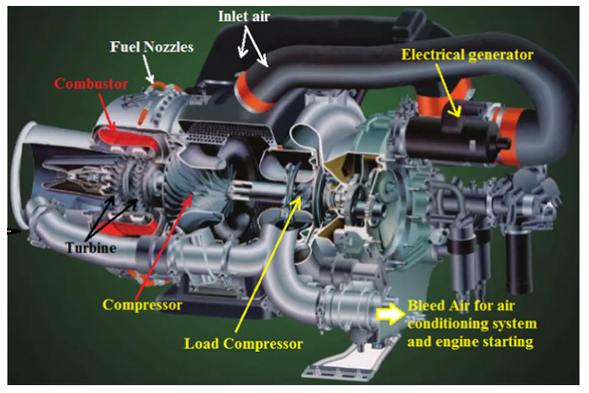
Taking the Hamilton Sundstrand APS5000 all-electric APU used in the Boeing 787 as an example, the structure of a typical all-electric APU is shown in
Figure 1 [
18]. Using the Honeywell 131-9 series APU employed in Boeing 737 and Airbus A320 aircraft as an example, the structure of a typical traditional APU is shown in
Figure 2 [
19]. The gas generators in both systems are single-shaft turboshaft engine structures. The principles and structures of the traditional APU and the all-electric APU are compared in the form shown in
Figure 3, where
represents power and
denotes rotor speed. The dashed line represents the components that are reduced in an all-electric APU as compared to the traditional APU. It can be seen that the all-electric APU eliminates two components that convert rotational power into pneumatic and hydraulic energy, resulting in a simpler structure. This simpler coupling and more direct relationship between the gas generator and starter/generator brings about both opportunities and challenges for fault estimation and FDI in the APU.
On one hand, this establishes a strong coupling relationship between the starter/generator and the gas generator, causing their faults to have significant impacts on each other and rendering starter/generator faults more critical [
8,
20]. This presents a new challenge for our FDI approach. On the other hand, it also offers opportunities to leverage this relationship to enhance our FDI methodology and performance. By utilizing information from one system, one can improve the estimates of the other system. This paper will focus on this opportunity and specifically illustrate how information from the starter/generator can be used to enhance the FDI performance of the gas generator.
Given that the energy output of a gas generator in an all-electric APU is solely reserved for the electrical part of the generator, an opportunity arises for us to precisely estimate the power output (shaft power) of the gas generator, thereby improving the accuracy of the fault diagnosis scheme in the gas generator.
The energy output of a traditional APU gas generator equals the sum of the energy consumed by the starter/generator that supplies electrical energy to the aircraft, the compressor that supplies the pneumatic energy, and the hydraulic pump that supplies the hydraulic energy. As a component of the electrical system, the power consumed by the starter/generator can be estimated through measurable electrical measurements. However, the energy consumed by the compressor and hydraulic pump is influenced by numerous factors, and obtaining accurate relevant parameters is a highly challenging task. Therefore, making a precise estimate of their power consumption is quite challenging. Moreover, due to the compact structure of the APU, installing torque or power sensors inside it poses significant challenges, which has always made estimating the power of the gas generator a complex task [
21,
22].
The advent of an all-electric APU offers a solution to the above problem. Without the compressor and hydraulic pump, one can estimate the power of the starter/generator with relative precision, thereby obtaining a fairly accurate estimate of power output of the gas generator. This information on the shaft power of gas generator can significantly enhance the estimation accuracy of states and the health parameters of the gas generator.
The feasibility of the above concept has already been demonstrated in other similar electro-mechanical systems, such as the hybrid electric vehicle and wind power generation industries. A range-extended electric vehicle (REEV) is an electric car powered by a battery and equipped with an on-board range extender generator, also known as an auxiliary power unit (REEV-APU). When the battery charge level is low, the range extender automatically starts and charges the battery. The REEV-APU consists of an engine and a generator, where the engine is solely responsible for driving the generator, which in turn supplies electrical power to the vehicle. Researchers in this field have conducted extensive studies on how to utilize the generator to estimate the engine’s shaft power and utilize power estimation to improve the parameter estimation and performance of the REEV-APU [
23,
24,
25]. Similarly, the wind power generation system primarily comprises a generator and a mechanical wind turbine, where the wind turbine, driven by wind power, serves as the prime mover that drives the generator to produce electricity. Researchers in this field have also conducted a substantial amount of research on how to utilize the generator’s signals, including shaft power information, to estimate the parameters, monitor the conditions, and diagnose faults in the wind turbine [
26,
27].
In this study, our aim and objective are to investigate why, how, and to what extent shaft power estimates from the starter/generator can enhance system state and health parameter estimation in an all-electric APU gas generator, thereby improving FDI performance.
5. Impact of Shaft Power Information from the Starter/Generator on the Gas Generator Fault Estimation Accuracy
This section evaluates the impact of shaft power information from the starter/generator on the estimation accuracy through a comparison between the PES and PENS. To facilitate this comparison, we develop MPESs (modified posterior estimates with shaft power information), a modified version of the PES model, and demonstrate its equivalence to the PENS model. This equivalence enables us to use MPESs as a bridge for effectively comparing PESs and PENSs. The results demonstrate that incorporating shaft power information significantly improves the estimation precision of each gas generator state and health parameter. This improvement becomes more pronounced under two conditions, namely, when using a more accurate state transition model or when estimating a larger number of health parameters.
5.1. Modified Posterior Estimate with Shaft Power Information (MPES) and Its Equivalence with PENS
After substituting Equation (9) for Equation (4) in the PES, we derive a modified estimate that is referred to as the MPES, and its algorithm is outlined as the Algorithm 3.
| Algorithm 3: Modified posterior estimates with shaft power information (MPES) |
Input : Engine augmented state space matrix:
, , , , ;
Posterior state estimate and covariance at :
, ;
Shaft power estimate from starter/generator:
;
Output : Posterior state estimate and covariance at :
, ;
Step 1 : Predict
1. Predict the prior estimate based on Equation (3);
2. Predict the prior estimate covariance based on
Equation (9);
Step 2 : Update
1. Obtain the Kalman gain based on Equation (5);
2. Update posterior state estimate based on Equation (6);
3. Update posterior state estimate covariance based on
Equation (7); |
The substitution that is outlined in Algorithm 3 reveals that the MPES is derived by leveraging the precise estimate from the starter/generator, without utilizing the corresponding covariance. Instead, the pre-set large value , used in Algorithm 2 for computing the PENS, is employed as the covariance. Consequently, the MPES represents estimates that are obtained by utilizing the accurate shaft power estimates from the starter/generator, albeit with minimal belief. Following this, we now introduce Theorem 1 to elucidate the equivalence between the MPES and PENS schemes.
Theorem 1. The estimation covariance and the Kalman gain in Algorithm 3 for achieving the MPES is equal to that in Algorithm 2 for achieving the PENS at each time step following
, as denoted by and
, where the superscripts and
correspond to the estimates and covariance of the MPES and PENS, respectively.
Proof. Since both algorithms for the PENS and MPES use Equations (4), (5), and (7), respectively, to compute the prior covariance and , the Kalman gain and , and the posterior covariance and , it follows that , , and when , provided that the system parameters and health parameters, as well as the measurements and inputs, are the same.
Thus, it can be inferred through recursive reasoning that and at each time step following when the system parameters, the initial Gaussian distribution of the system states and health parameters, as well as the measurements and inputs are the same.
This completes the proof of the theorem. □
Here, we have demonstrated the equality of the covariance and the Kalman gain between the PENS and MPES. Next, we will demonstrate that the estimates of the PENS and MPES are also the same under the conditions.
Theorem 2. Assuming that is bounded for any when
, where
represents any row of the matrix and the subscript
refers to the matrix element at the corresponding row and column, then it follows that as
, the difference between
and
converges to zero following the initial time
.
Proof. By expanding Equations (4) and (7), one can express the posterior estimate variance of the PENS as follows:
It follows that all the three parts in Equation (10) are positive semi-definite matrices. Considering that when is bounded for any , it follows that as .
Using Equation (6) and Theorem 1 above, and considering the same inputs and measurements, one can derive
Based on the result that as , it can be inferred that if , thus as .
Then, through recursive reasoning, one can derive that as , for each time step following the initial time , under the assumptions of the theorem. This completes the proof of the theorem. □
Theorem 2 implies the practical equivalence of estimates between the PENS and MPES. This is due to the fact that the is a large number, as previously described, and when PENS is effective (signifying that the estimation error is not significantly large, i.e., is not a large value for any ), then and are almost the same.
By combining the covariance equivalence that is presented in Theorem 2 with the equivalence of estimates that is outlined in Theorem 3, one can conclusively establish the equivalence between the PENS and the MPES.
In this subsection, we proposed the MPES and demonstrated the equivalence of the PENS and MPES. Subsequently, we will assess and compare the estimation accuracy of the PENS and PES by examining the accuracy between the MPES and PES.
5.2. Comparative Estimation Accuracy Analysis of PENS and PES
In this section, we will demonstrate and derive the differences in accuracy between the PES and PENS. Given the demonstrated equivalence between the PENS and MPES in the previous subsection, we can assess the estimation accuracy of the PES relative to the PENS through a comparison with the MPES.
Theorem 3. Assuming that the shaft power estimates and corresponding covariances from starter/generator, which are provided to the PES, are consistent with the actual system and in each time step, then it follows that
for any and time step following , where and
, representing the expected squared estimation errors for the th estimate of the MPES and PES, respectively.
Proof. We first denote
and
as the covariance of estimation error (CEE) [
47] of the MPES and PES as follows:
where subscript
denotes the expected squared estimation error matrix.
The proof can now be transformed into demonstrating that for any given and time step subsequent to , under the stipulated assumptions.
Given that the parameters that are provided to compute the PES are all consistent with the actual system, it follows that the posterior covariance of the PES is equal to its CEE, namely
holds for any time step following
. Consequently, based on Equation (7), the CEE of the PES, as denoted by
, can be expressed as follows [
47]:
where
Due to the lack of actual shaft power distribution information in the calculations for the MPES, the posterior estimate of the MPES is not the CEE of the MPES. The CEE of the MPES is presented as follows [
48]:
where
By utilizing Equations (14) and (15), the expression for
can be derived as shown in Equation (16), as follows:
From Equation (16), it can be observed that when
, the right-hand side of Equation (16) consists of two positive semi-definite matrices, resulting in
, where
represents that
is a positive semi-definite matrix, because we have
Therefore, through the application of recursive reasoning, it can be concluded that, given and the same actual initial distribution implying , along with other assumptions outlined in the theorem, the inequality is maintained at any time step following . Hence, based on Equation (16), one can derive that holds under the same conditions.
Based on the properties of positive semi-definite matrices and the definition of the CEE, one can conclude that for any index and for all time steps subsequent to , given the assumptions that are specified in the theorem. This completes the proof of the theorem. □
We next explore the conditions under which equality is consistently achieved in the inequality . From Equation (16), it follows that for the inequality to consistently hold, the th row of the matrix must be zero. Referring to Equation (5), it is observed that if the matrices and do not contain any rows entirely composed of zero elements, and matrix does not have any columns entirely composed of zero elements, then the matrix will not have any rows consisting solely of zero elements. Therefore, by combining the equivalence between the PENS and MPES as demonstrated in Theorems 1 and 2, we can conclude that for any under the given estimation scenarios.
Building on the conclusion and the definitions provided in
Section 4 for Scenarios 1 and 2, as well as for the PES and PENS, we demonstrate that the use of shaft power information from the starter/generator can improve the accuracy of estimating each system state and health parameter. This improvement will consequently enhance the achievable FDI capabilities.
From the proofs of Theorems 1–3, it can be observed that the improvement in the estimation accuracy for each state and health parameter, due to the shaft power information, is attributable to the intrinsic characteristics of the all-electric APU gas generator. The influence of the shaft power on each state enhances the estimation of each system state. The fact that each measurement is influenced by at least one state, and that, in turn, each health parameter can affect at least one measurement, improves the estimation of each health parameter.
Additionally, the proofs of Theorems 1–3 reveal that the capability of shaft power estimates from the starter/generator to enhance estimation accuracy lies in providing more accurate prior estimates. This improvement becomes more pronounced with the enhancement of the accuracy of the model state transition representation. On the other hand, as the number of health parameters increases, the uncertainty and difficulty of the estimation also increases, thereby elevating the importance of accurate prior estimates. This amplifies the advantages of estimates that utilize shaft power information.
Consequently, as the accuracy of the state transition representation or the number of health parameters in the gas generator model increases, the significance of the improvement in the estimation accuracy of system states and health parameters, enabled by the shaft power information from the starter/generator, becomes more pronounced. A detailed demonstration of this is provided in
Section 6.
In this section, we have demonstrated that incorporating shaft power estimates from the starter/generator can improve the estimation accuracy of each state and health parameter of the gas generator, thereby enhancing the achievable FDI performance. We also analyzed the relationship between this improvement and the unique characteristics of the all-electric APU. Additionally, we examined the aspects that can influence the degree of achievable performance improvement. The subsequent section presents simulation results to further substantiate and demonstrate our proposed methodology.
6. Simulation Results
In this section, we utilize Monte Carlo simulations to demonstrate the impact of shaft power estimates from the starter/generator on the FDI performance of an all-electric APU gas generator. Furthermore, we investigate the correlation between this impact, model accuracy, and the number of health parameters.
First, we introduce the model of the gas generator that is used in our study. Subsequently, we present and compare the confusion matrices for the FDI in scenarios both with and without shaft power estimates derived from the starter/generator. These comparisons support our conclusion that the incorporation of shaft power information significantly enhances the achievable FDI performance of gas generators.
We also present comparison results for the FDI after adjusting the noise level in the gas generator model and the number of health parameters to be estimated. The results indicate that improvements in the FDI performance are more pronounced by utilizing a more accurate model or a greater number of health parameters.
In this study, gas-path faults are selected as the research focus, and a corresponding gas generator fault model is developed as follows:
where
and the subscript
represents the reference steady-state value,
represents the rotor speed (single shaft),
represents the measured rotor speed,
represents the measured compressor outlet temperature,
represents the measured compressor outlet pressure,
represents the measured turbine outlet temperature, and
,
,
, and
, respectively, represent the degradation of compressor efficiency, compressor flow capability, turbine efficiency, and turbine flow capability.
The above linear model formulation is a typical representation of single-shaft all-electric APU gas generator gas-path fault models commonly employed in the industry [
40,
49,
50]. This model was derived by linearizing a component-level nonlinear all-electric APU model developed using GasTurb [
51]. The component-level model’s parameters and design are based on the Hamilton Sundstrand APS 5000, which is a mainstream single-shaft all-electric APU widely used in the current field [
18]. The modeling approach employs GasTurb-based dynamic link library technology [
52,
53,
54], which enables the simulation of gas-path faults in the gas generator. The model’s validity has been confirmed through validation using widely recognized industry software and relevant literature. To maintain the shaft speed at its nominal value, a proportional–integral (PI) controller was also designed and incorporated.
Gas-path faults represent a critical area of focus in the field, as such faults significantly affect the efficiency and flow capacity of major rotating components [
40,
49,
50]. The linearized model described above constitutes a typical all-electric APU gas generator gas-path fault model, with rotational speed as the state variable and the health parameters
,
,
, and
used to quantify the severity of gas-path faults. These four parameters represent the efficiency and flow factors of the compressor and turbine, respectively, as defined in Equations (20) and (21). In a healthy state, these parameters have a baseline value of 1. Deviations from this baseline can indicate changes in efficiency and flow due to gas-path degradation. The gas-path degradation of compressors and turbines is primarily caused by issues such as blade corrosion, erosion, fouling, and tip wear, among others, which lead to alterations in blade parameters and overall performance. Typically, compressor degradation results in decreased efficiency and reduced flow, whereas turbine degradation is characterized by decreased efficiency albeit with increased flow [
55,
56,
57,
58,
59]. Specifically, we have
where
and
denote the actual efficiencies of the compressor and turbine, respectively,
and
represent their nominal efficiencies,
and
indicate the actual flow rates, and
and
correspond to the nominal flow rates.
It is evident that this model conforms to the model structure and satisfies all assumptions outlined in
Section 3, thus enabling its application for validating the effectiveness of our analytical conclusions, while also confirming the rationality of our related assumptions. Based on the values of these health parameters, degradation is categorized into four distinct health conditions, namely healthy, minor fault, medium fault, and severe fault. These conditions are detailed in
Table 1.
It is worth noting that the above classification of healthy, minor fault, medium fault, and severe fault states does not carry any special physical considerations. This classification serves to differentiate fault severity levels, enabling us to evaluate PES-based and PENS-based approaches through their ability to distinguish different fault magnitudes. Combined with the assessment of fault estimation accuracy, this provides a comprehensive evaluation of both fault estimation and the FDI capabilities of PES-based and PENS-based approaches. This helps validate our theoretical framework by examining whether fault estimation and diagnosis with shaft power information indeed outperforms those without it, and whether the factors affecting this shaft power information-induced improvement align with our analysis. Such fault classification and testing methodology has been widely adopted in various aero gas turbine fault estimation and diagnosis studies to compare the estimation and diagnostic capabilities of different approaches [
60,
61,
62,
63].
Case 1: We set measurement noise
and process noise
to be 0.5% of the reference steady-state values of states and measurements, respectively. We conducted 100 Monte Carlo simulation runs for each condition, as shown in
Table 1. Each simulation began completely healthy, namely all health parameters were set to 1, and gradually degraded to the target condition. We used the PES and PENS algorithms as described in
Section 4 to estimate health parameters. Subsequently, we performed an FDI scheme based on these estimation results to identify the health condition associated with each degradation.
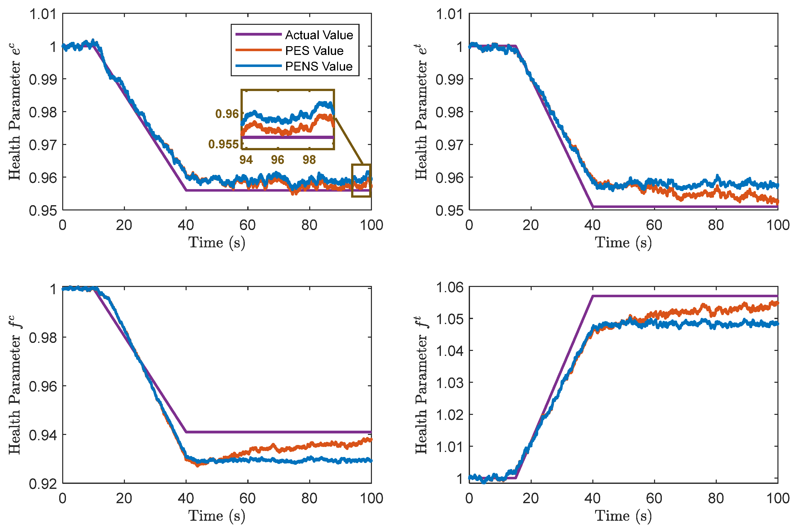
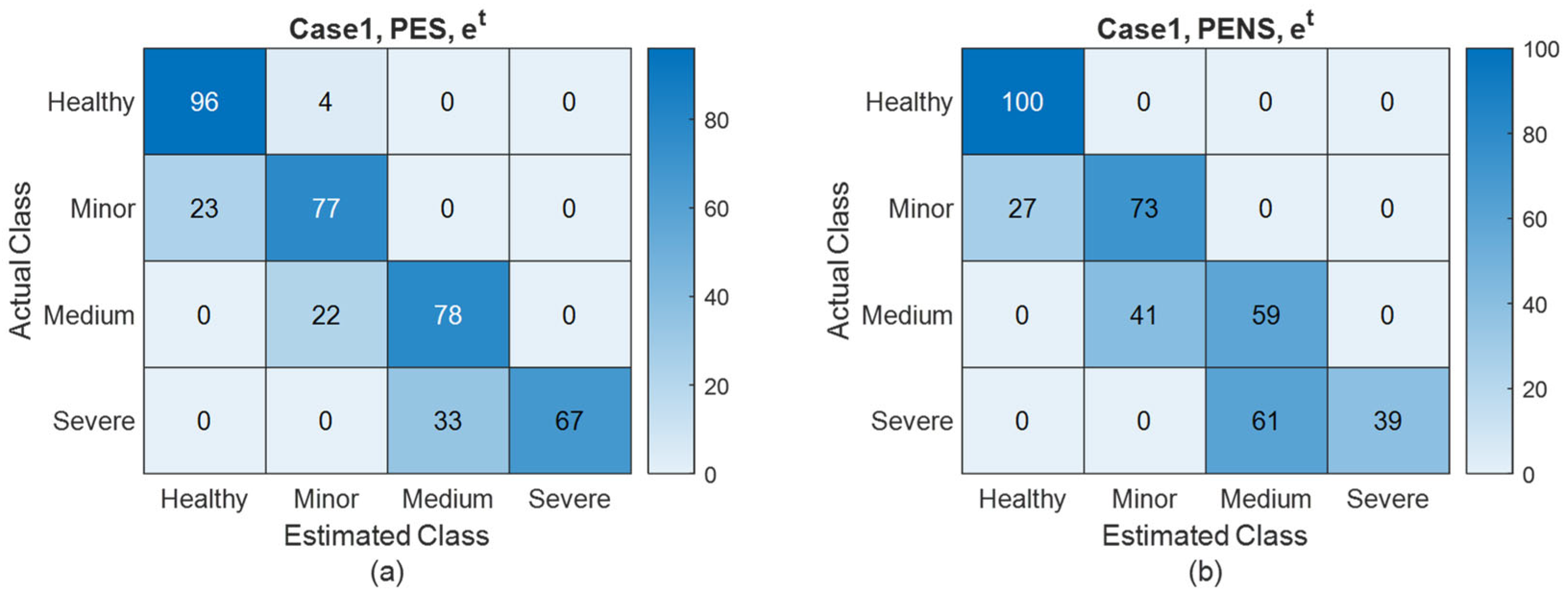
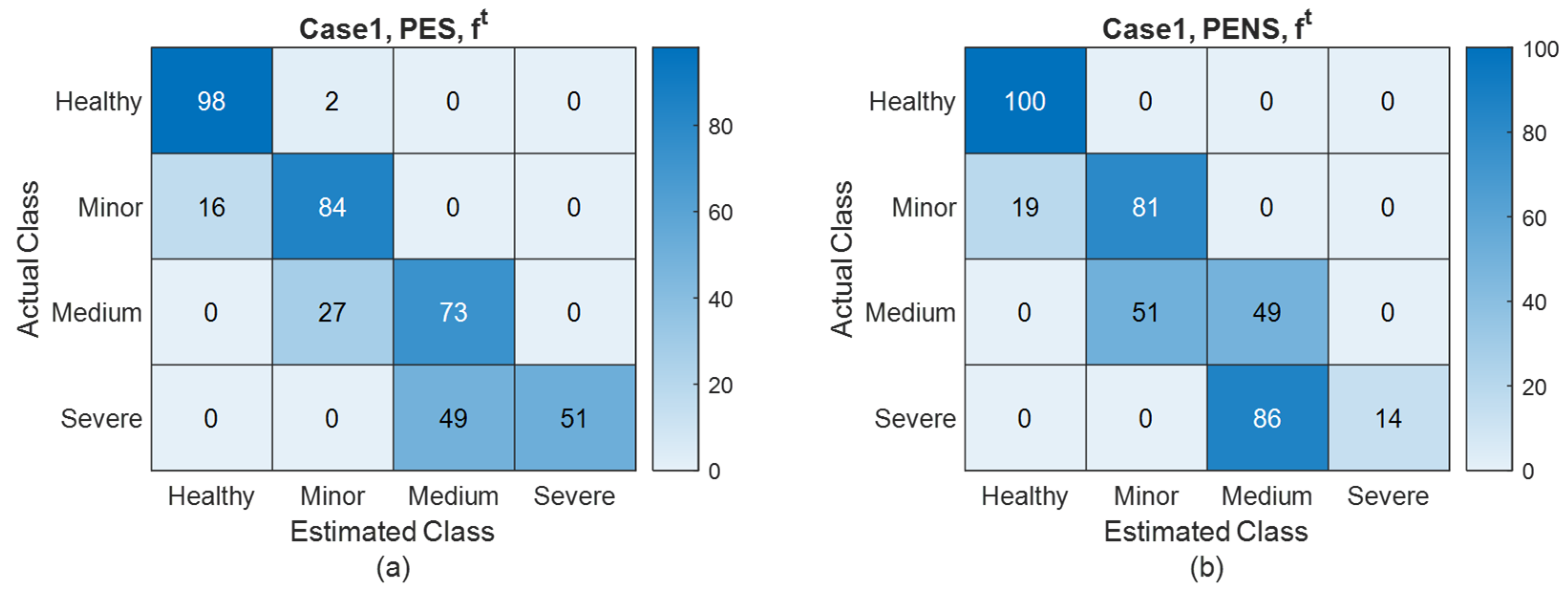
Figure 4 illustrates the dynamic estimation results from a representative simulation sample.
Table 2 shows the estimation accuracy of the PES and PENS, where RMSE represents the root mean square error.
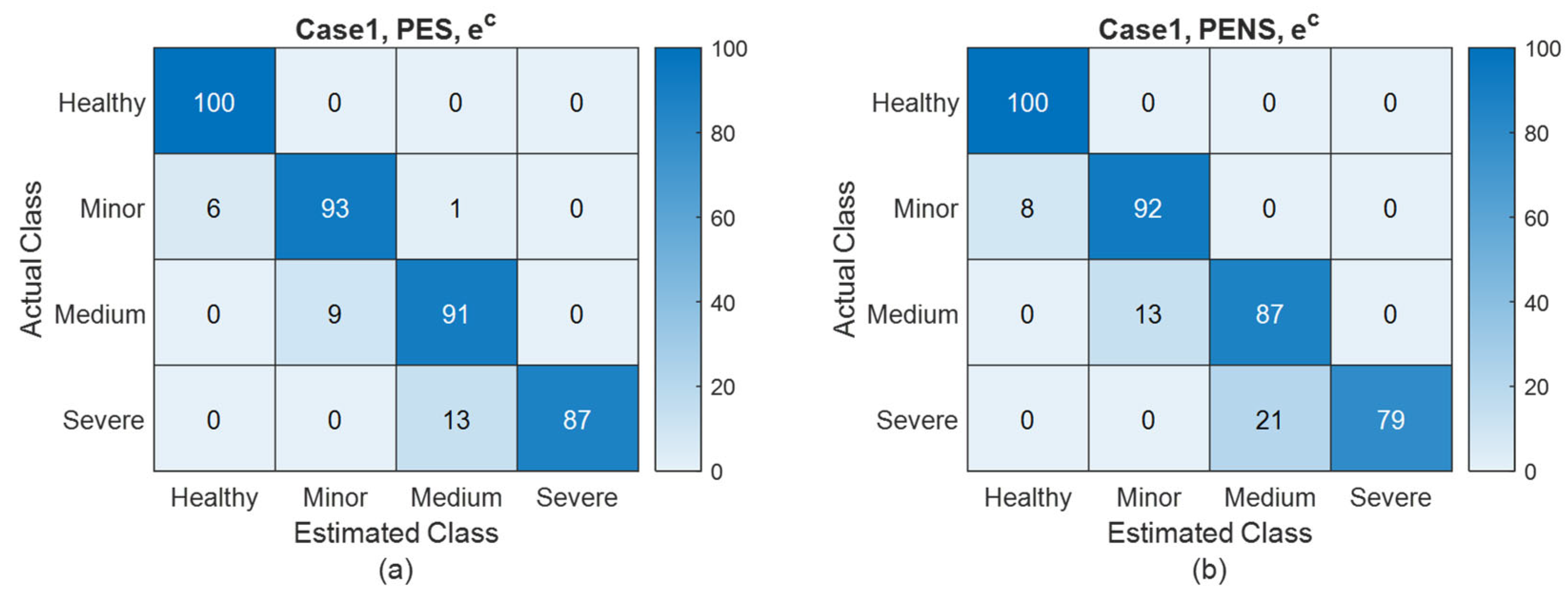
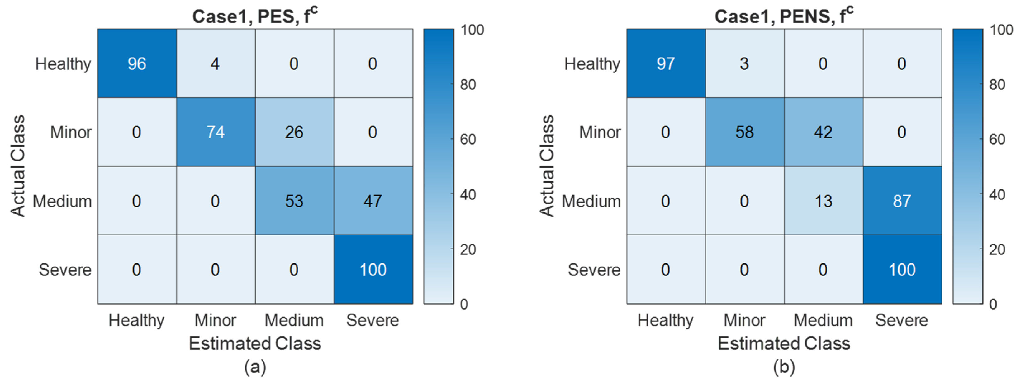
Figure 5,
Figure 6,
Figure 7 and
Figure 8 present FDI confusion matrices based on the PES and PENS for
,
,
, and
, respectively.
Figure 4 and
Table 2 demonstrate that the PES significantly outperforms the PENS in terms of estimation accuracy for each state and health parameter. Also, from
Figure 5,
Figure 6,
Figure 7 and
Figure 8, we can observe that FDI utilizing the PES demonstrates superior performance as compared to FDI based on the PENS, particularly as fault severity escalates.
For the healthy condition, the FDI based on both the PES and PENS demonstrates comparable performance. This can be attributed to the fact that a completely healthy system does not exhibit any dynamic changes in health parameters due to degradation. Each parameter consistently maintains a value of 1, thereby reducing the complexity of the estimation and resulting in similar FDI performance.
However, for minor, medium, and severe fault conditions, the FDI systems that utilize PESs exhibit markedly superior performance as compared to those using PENSs. This superiority is evidenced by higher detection rates as well as lower false positive and negative rates, particularly in the context of higher severe faults. Consequently, the simulation results from Case 1 substantiate the conclusion in
Section 5 that shaft power information can improve the estimation accuracy of each state and health parameter, resulting in an enhancement in the performance of the FDI scheme.
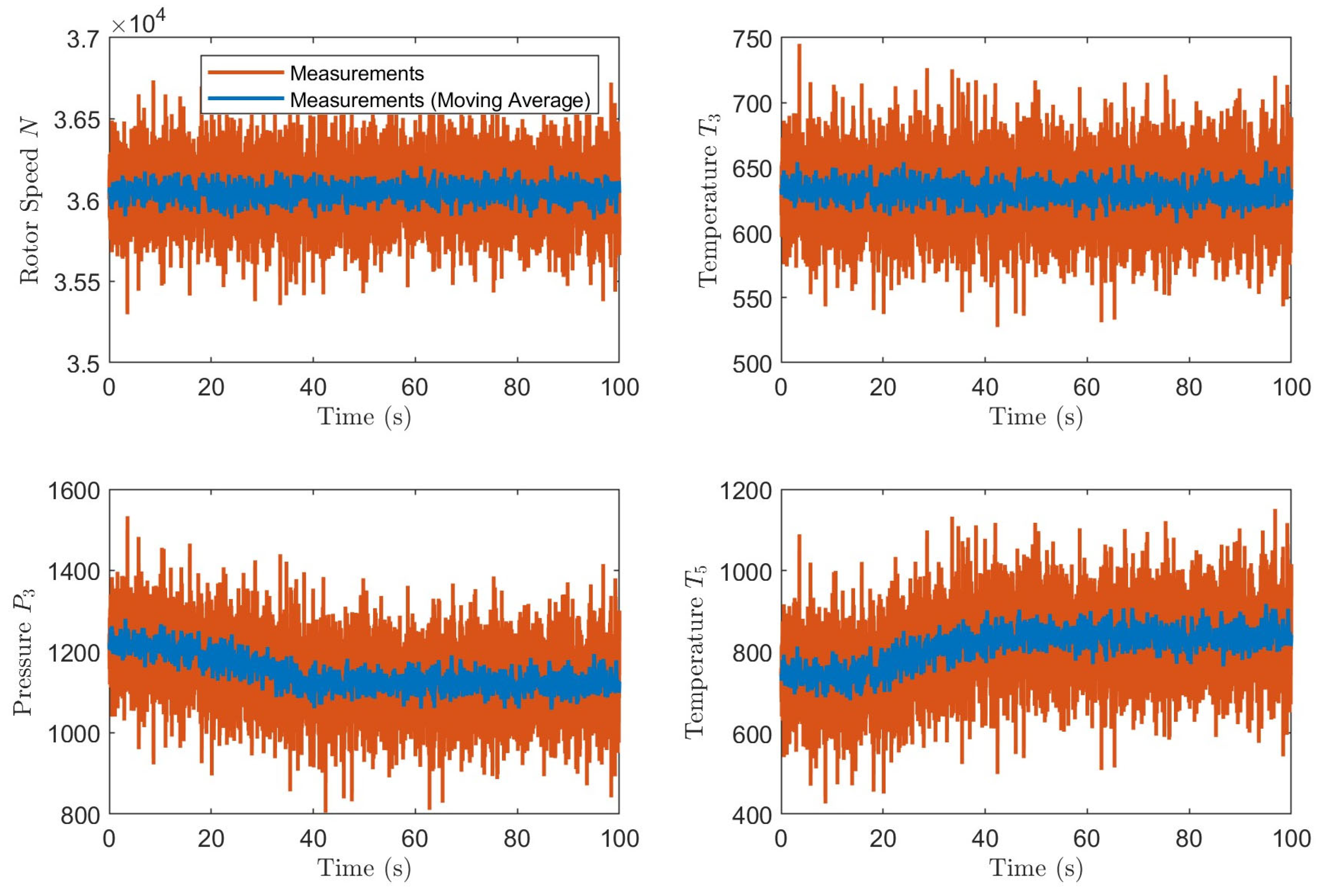
Next, we analyze the changes in system measurements, including the state variable (rotor speed) and other measured parameters, during gas-path faults. Taking the degradation profile shown in
Figure 4, we set the shaft power output to remain constant and examine the resulting system measurements as illustrated in
Figure 9. The red lines represent raw measurements while the blue lines show the moving average values to better illustrate the trends, as the original measurements (red) are affected by state and measurement noise.
From the figure, we can observe that the rotor speed (state variable) exhibits minimal variation. This is because APU gas generators typically operate under fixed-speed control logic at specific operating conditions [
64]. As mentioned in the model description at the beginning of this section, a PI controller was implemented to maintain the nominal speed.
Examining the system parameters in Equations (18) and (19) and the degradation curves in
Figure 4, we notice that for this particular degradation profile, the health parameters’ effects on
largely cancel each other out, resulting in minimal
variation. However, this limited variation is specific to this sample’s degradation rate and should not be considered universal.
For
and
, since their influences cannot be mutually canceled, we observe significant changes after degradation. The degraded compressor performance results in reduced compression capability, leading to lower pressure ratio for the same temperature rise. This decreased gas work capability means that to maintain the same power output, higher temperatures and increased fuel consumption are required. Consequently, we observe decreased compressor outlet pressure
and elevated turbine outlet temperature
. For more detailed analysis of degradation effects on system performance, readers are referred to the relevant literature [
30,
32,
38,
51].
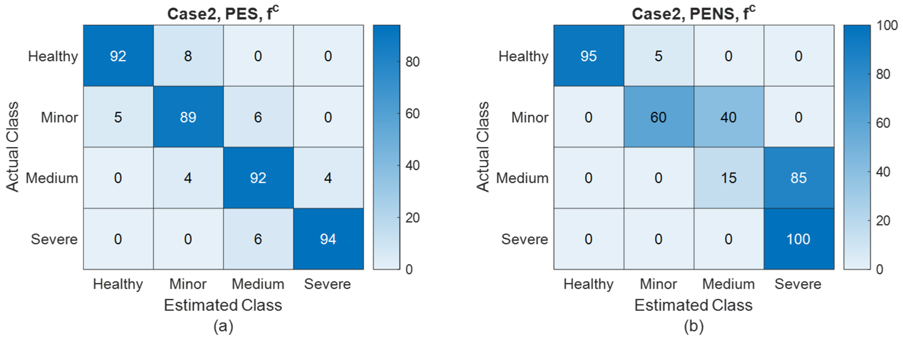
Case 2: We now reduced the process noise
to 0.1% of the reference steady-state values of the system states, while keeping all other parameters the same as in Case 1. Subsequently, we also conducted 100 Monte Carlo simulation runs for each condition, as shown in
Table 1.
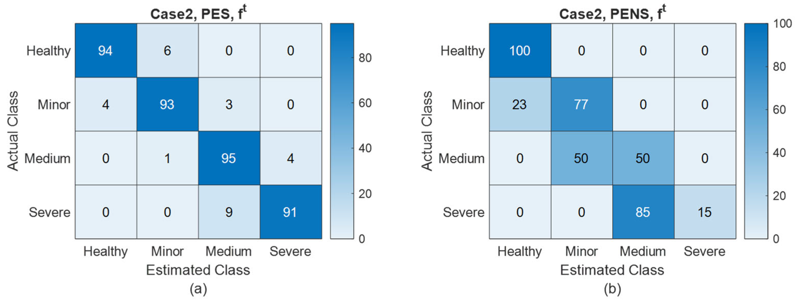
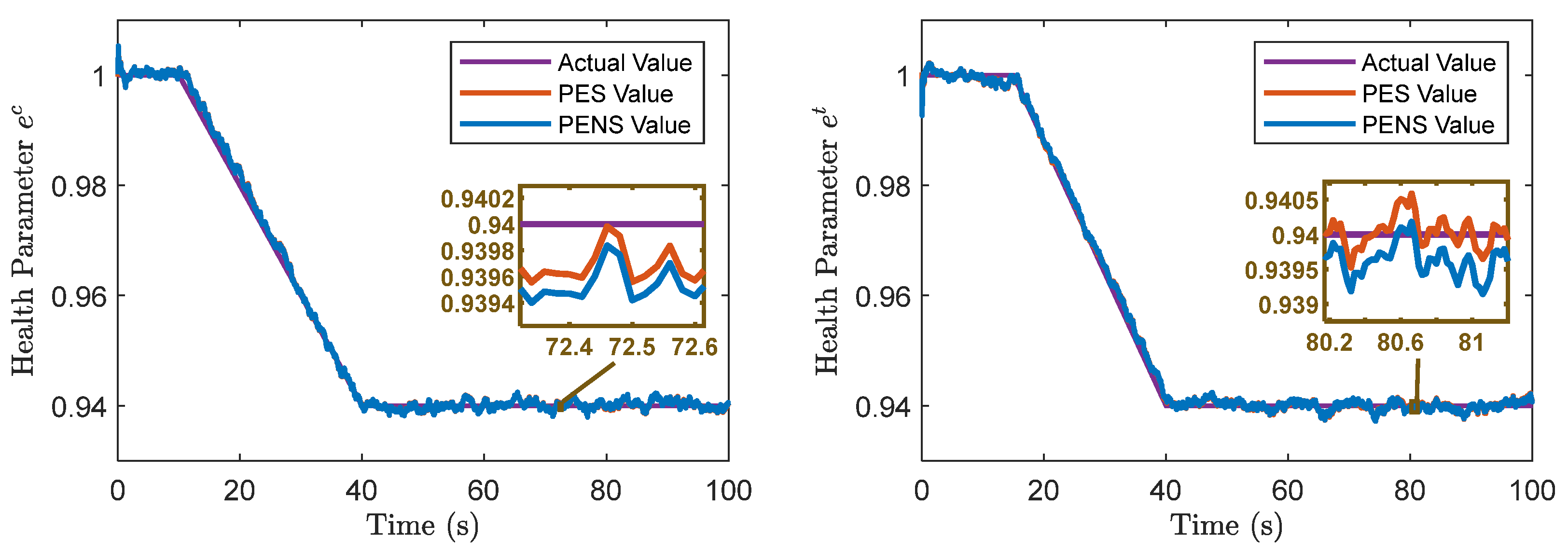
Figure 10 illustrates the dynamic estimation results from a representative simulation sample. The estimation accuracy of the PES and PENS, along with corresponding FDI results, are provided in
Table 3 and
Figure 11,
Figure 12,
Figure 13 and
Figure 14.
Figure 10 and
Table 3 demonstrates the estimation accuracy and FDI capabilities in scenarios both with and without access to shaft power information, given a more accurate model. Comparing
Table 3 with
Table 2 shows that the accuracy of the PES increases with the use of a more accurate model, while the accuracy of the PENS remains nearly unchanged under the same conditions. This leads to a larger accuracy advantage for the PES over the PENS. It can be inferred that increased accuracy in the model state transition representation enhances the positive impact of power shaft information on the accuracy of health parameter estimation.
Note that a more accurate state transition representation leads to a more effective utilization of power shaft information, resulting in improved prior estimations and, ultimately, enhanced overall accuracy and FDI performance. However, in scenarios lacking shaft power information, the improvement in the accuracy of the state transition representation does not significantly enhance the estimation accuracy. Without the shaft power information, state transition representation plays a limited role in estimating states and health parameters, which primarily rely on the observation equation. Consequently, simulation results for Case 2 show that a more accurate model enhances the positive impact of power shaft information on the accuracy of achievable health parameter estimation results.
Case 3: We assume that degradation of the compressor and turbine simultaneously occurs in terms of efficiency and flow, and there exists a known proportional relationship as given by Equation (22) [
57]. Given that
are known fixed values, the description of the gas generator gas-path degradation can be reduced from the four independent health parameters
to the two independent variables
, as specifically shown in Equation (22). Next, we set the same noise level as in Case 2 and keep all other parameters unchanged. Subsequently, we also conducted 100 Monte Carlo simulation runs for each condition, as shown in
Table 1.
Figure 15 illustrates the dynamic estimation results from a representative simulation sample. The estimation accuracy of the PES and the PENS, along with the corresponding partial FDI results, are detailed in
Table 4 and
Figure 16 and
Figure 17.
where
respectively, denote the known fixed correlation coefficients between the efficiency factor and the flow factor of the compressor and turbine, respectively.
Figure 15,
Figure 16 and
Figure 17 provide estimation accuracy and FDI performance when fewer health parameters are estimated by using the same number of measurements, indicating a relatively higher sufficiency of information for estimating health parameters. In
Table 4, it follows that the estimation accuracies of the PES and PENS are nearly the same. This similarity can be attributed to the fact that estimating fewer parameters while maintaining the same number of measurements results in relatively less uncertainty in estimations. This diminished uncertainty arises from the assumption in Case 3 of a determined relationship among health parameters, thereby narrowing the possible distribution of parameters given the same measurements. Consequently, when uncertainty is lower, the contributions of shaft power estimates from the starter/generator to enhancing the accuracy of health parameter estimation are minimal. Furthermore, similar FDI performance based on both the PES and PENS, as per
Figure 16 and
Figure 17, further supports our conclusion.
Consequently, comparisons between Cases 3 and 2 indicate that the contribution of shaft power information in improving the estimation accuracy of system states and health parameters becomes more significant when more health parameters are estimated.
In
Table 5 below, we present the macro averages of precision, recall, and F1 score for FDI based on the PES and PENS across different health conditions in Case 1, Case 2, and Case 3. From the data in
Table 5 for Case 1, it is evident that the PES outperforms PENS due to its use of precise shaft power information. Furthermore, the data in
Table 5 for Case 2 show that as the model accuracy improves, the advantages of the PES become more pronounced. However, data in
Table 5 for Case 3 also indicate that when the number of health parameters to be estimated decreases, the importance of additional shaft power information diminishes due to reduced system uncertainty, resulting in similar performance between the PES and PENS.
It follows that the relative advantage of the PES over PENS lies in its significant accuracy benefits when measurement information is relatively insufficient, the number of health parameters to be estimated is large, or the model accuracy is high. On the other hand, the relative advantage of the PENS is that it does not require additional precise shaft power information provided by a generator, making it easier to deploy. It also performs well when model accuracy is not high or the number of health parameters to be estimated is small. Therefore, the choice between the PES and PENS should be based on the specific scenario and application under consideration.
The above Monte Carlo simulation runs and related analyses have confirmed our conclusion that incorporating shaft power information can enhance the estimation accuracy of each state and health parameter, thereby improving the FDI performance. These improvements are especially pronounced with a more accurate model or when more health parameters are involved, as discussed in
Section 5.
In this study, linear degradation patterns are employed for validation purposes. This choice is justified as our focus is on fault estimation rather than fault prediction, and the proposed estimation method is not significantly dependent on the specific form of the degradation curve. As long as the degradation process is gradual, the estimation accuracy remains robust across different degradation patterns. This is evidenced through our Monte Carlo simulations, where various degradation rates are tested despite the linear form. While more complex stochastic degradation models exist in the reliability literature, linear degradation models are commonly used in fault estimation studies [
30,
65,
66] due to their ability to effectively validate estimation algorithms.
It should be noted that the above model used for simulation validation is based on a single-shaft all-electric APU gas generator gas-path fault model referenced from the currently prevalent Hamilton Sundstrand APS 5000. However, our analysis and conclusions are derived through mathematical analysis and are of general applicability. The analytical framework and conclusions presented herein are valid for any aviation gas turbine and associated faults that conform to the model specifications and assumptions established in
Section 3, including all-electric APUs with alternative configurations and hybrid electric aircraft power systems that exhibit analogous structural characteristics.
Furthermore, it should be emphasized that this study investigates the theoretical upper bounds of estimation capability rather than specific implementation approaches. While our theoretical derivation and simulation validation employ Kalman filtering, we utilize it solely for its optimal estimation properties to establish the best achievable estimation accuracy under ideal conditions, rather than as a proposed implementation method. Our analysis demonstrates that when a system satisfies our model assumptions, the theoretical upper bound of estimation accuracy with shaft power information is higher than that without such information, and this advantage becomes more pronounced when the model is more accurate or when more health parameters need to be estimated. This fundamental conclusion about theoretical limits is independent of practical implementation aspects such as specific estimation methods, system identification, or parameter acquisition procedures.


