1. Introduction
The performance of fuel electro-hydraulic servo valves, the core actuating elements of modern hydraulic control systems, directly determines the reliability and control accuracy of aerospace and other major equipment [
1]. In a fuel electro-hydraulic servo valve, a key component with extremely high precision requirements, there is usually only 5–15 μm clearance between the spool and the valve body, and under the special working conditions of low viscosity and high pollution of the fuel medium, micron-sized particles of contaminants are very likely to cause serious failures such as spool motion stagnation [
2,
3,
4]. Statistics show that the aviation hydraulic system failure cases caused by particle contamination comprise up to 82% of the total number of failures, of which sliding valve gap contamination hysteresis accounts for more than 60% [
5,
6,
7]. This micro-mechanism of dynamic friction sub-failure triggered by particle accumulation has become a bottleneck problem restricting the development of high-end hydraulic components.
Liquid–solid two-phase flow analysis technique provides an important research tool for revealing the particle dynamics behavior in the interstitial space. In the traditional approach, the CFD-DEM coupling strategy accurately describes the particle–fluid momentum exchange process through the Eulerian–Lagrangian framework [
8,
9,
10]. However, the classical CFD-DEM faces computational efficiency dilemma in micro- and nanoscale flow simulations. Barigou et al. [
11] improved the computational strategy by the SPH meshless method, which successfully improved the spatial resolution of particle–wall interactions to the submicron level. For the complex wall conditions, the PPIC-VOF model developed by Mohseni et al. [
12] realizes the multi-scale coupling calculation of multiphase flow and solid particles, which opens up a new way for the liquid–solid coupling study under a rough surface. At the experimental research level, the particle trajectory tracking system based on PIV [
13] and microscopic high-speed camera technology [
14] provides a reliable means for the validation of the theoretical model.
In recent years, scholars have made a series of breakthroughs in the field of hydraulic component contamination mechanism research. Mittal et al. proposed an immersed boundary calculation method, which can calculate the motion characteristics of particles in the flow field in a cross-scale basin [
15]. Terrell et al. proposed a hybrid modeling method combining particle dynamics model and dynamic model and obtained the motion trajectory of the nanoabraded particles in the abrasive fluid [
16]. Vito Tic et al. analyzed the motion characteristics of contaminated particles in a hydraulic tank based on the Eulerian–Lagrangian liquid–solid two-phase flow method [
17], and Yohsuke Tanaka et al. used a high-resolution PIV test system to record the particle trajectories in a Kamen vortex street and obtained the interaction between the Kamen vortex street and the motion of particles [
18].
It is worth noting that, although these results have greatly improved the understanding of particle dynamics, the existing studies generally assume that the moving subsurfaces have ideal geometric characteristics, the research models are still based on smooth surfaces, and there is a theoretical gap in the consideration of the transport mechanism of particulate matter under rough surfaces.
This paper focuses on the anti-pollution design needs of fuel electro-hydraulic servo valves and carries out the research on the mechanism of liquid–solid coupling action under rough surfaces. In the second part, the liquid–solid two-phase flow study method is used to analyze the force on sensitive particles in the interstitial flow field. In the third part, different rough slide valve gap models are established by characterizing the rough surface morphology through the numerical simulation method of the W-M fractal model. In the fourth part, the particle transport characteristics in the rough slide valve gap are obtained. In the fifth part, the particle transport characteristics of the rough slide valve gap are analyzed. In order to verify the accuracy of the simulation model, experimental validation is carried out in the sixth part. The seventh part is the conclusion.
2. Force Analysis of Sensitive Particles in Interstitial Flow Fields
2.1. Effect of Particles on Slide Valves
A schematic diagram of a typical fuel electro-hydraulic servo valve is shown in
Figure 1. The electro-hydraulic servo valve generally consists of three main components: a torque motor, a hydraulic amplifier, and a feedback mechanism. This type of servo valve uses fuel oil as the working medium; however, due to the absence of a circulation filtration system, the fuel often contains a high level of contaminants. If an excessive number of particles migrate and accumulate within the internal gaps, these sensitive particles can cause friction and wear on the spool surface during its operation. This can directly affect the performance and service life of the hydraulic system and may even lead to spool jamming, resulting in the failure of hydraulic components and compromising the normal operation of the system.
2.2. Liquid–Solid Two-Phase Flow Research Methods
The Eulerian–Lagrangian method treats the liquid phase as a continuous medium and uses the Eulerian method to analyze the motion processes of the fluid. The solid-phase particles are treated as discrete phases, the motion of the particles is described using the Lagrangian method, and the two methods are coupled to each other by interacting forces (e.g., trailing forces, lift forces, etc.).
Liquid phase governing equations in this method, the fluid is considered to be a continuous phase. Consequently, the Navier–Stokes equations are employed to describe the conservation of mass and momentum of the fluid. The mass conservation equation for the liquid phase is as follows:
where
—density of the fluid (kg/m
3);
—time (s);
—fluid movement speed (m/s).
The momentum conservation equation for the liquid phase is
where
—fluid pressure (Pa);
—fluid dynamic viscosity (Pa-s);
—gravity acceleration (m/s2);
—the force of the particles on the fluid (N).
The Euler–Lagrange method is predicated on the assumption that solid-phase particles are to be regarded as discrete phases. These particles are then described by the Lagrange method, which involves analyzing the position, motion, velocity, and acceleration of the particles, as well as the force exerted on them by the fluid. The equations of motion of the particles are obtained through Newton’s second law. The trajectory of the particles in the flow field is then analyzed, thus yielding the equation of motion of the particles:
where
—pellet mass (kg);
—velocity of particle movement (m/s);
—trailing force (N);
—the force of gravity (N) on the particles;
—the buoyant force (N) on the particles;
—pressure rise force on particles (N).
2.3. Particle Force Analysis
The motion of the particles in the rough slide valve gap is analyzed by treating the oil as a continuous phase and the particles as a discrete phase, based on the basic Eulerian–Lagrangian calculation method.
Derived from Newton’s second law, the equation of motion for the particle is thus established:
The main force diagram of the particles is shown in
Figure 2. The movement of the sensitive particles within the flow field of the slide valve gap is primarily influenced by gravity, buoyancy, traction, and Saffman lift.
Gravity is an objective force on any object that has a direct effect on the trajectory of the particles. The formula for the force of gravity on a particle is
The buoyant force exerted on the particles is equivalent to the force of gravity, which is a constant force, and the direction of the buoyant force is antithetical to the force of gravity. The formula for the buoyant force on the particles in the oil is as follows:
The expression for the trailing force on a single circular sensitive particle in the flow field in the slide valve gap flow field model is given by
where
denotes the coefficient of resistance.
The drag coefficient of round particles moving in a fluid is frequently principally influenced by the particle Reynolds number. The majority of scholars have derived an empirical formula for calculating the drag coefficient by experimental methods as follows:
where
represents the particle Reynolds number in the flow field and is expressed as
The diameter of the particles under scrutiny in this study is 1 μm, with subsequent analysis of the transport of particles at varying flow rates. The drag coefficient calculation formula is thus selected when the particle Reynolds number is less than 800. The trailing force calculation formula employed in this study is as follows:
When a particle moves in a flow field with a velocity gradient, the pressure in the upper part of the particle is lower than the pressure in the lower part because the velocity in the upper part of the particle is higher than the velocity in the lower part, and the particle will be subjected to a lifting force, which is known as the Saffman force.
The expression for the Saffman force is
3. Different Roughness Slide Valve Gap Modeling
3.1. Numerical Simulation of the W-M Fractal Model
For the surface of the servo valve spool, the numerical simulation method of the W-M function fractal model is used to characterize the rough surface topography and analyze the relationship between the two-dimensional fractal parameters and the complexity of the surface contour and topography, and the fractal dimension D and the scale parameter G jointly affect the complexity of the function and the overall height. The function expression is
where
the value of the fractal function, expressed in the independent variable x at the height of the two-dimensional profile; G control function of the overall scale or amplitude; D is the two-dimensional profile of the fractal dimension, describing the complexity of the curve, and 1 < D < 2; n is the infinite series of the number of terms;
is the smallest infinite series of the terms; x is an independent variable that can be expressed as a machining surface simulation of the sampling length;
is the scale factor, the value of which is a constant; and
> 1. In practical engineering problems, it is often made that
= 1.5.
Figure 3 and
Figure 4 illustrate the impact of fractal dimension D and scale factor G on the W-M function curve and surface roughness, respectively. Increases in the fractal dimension D have been shown to result in a decrease in vibration amplitude, accompanied by an increase in vibration intensity and complexity. This corresponds to a flatter and finer textured machined surface. Furthermore, it is evident that a decrease in the scale factor G results in a concomitant decrease in the contour value of the curve, whilst the magnitude of both variables remains constant. It can be demonstrated that if the scale factor G is altered, the morphology and complexity of the curves remain unchanged, and the self-similarity also stays the same. This indicates that the scale factor is the main factor affecting the height of the surface roughness. Consequently, when describing different surface roughness, it is possible to effectively control the height of the rough surface by adjusting the scale factor.
3.2. Modeling of Different Roughness
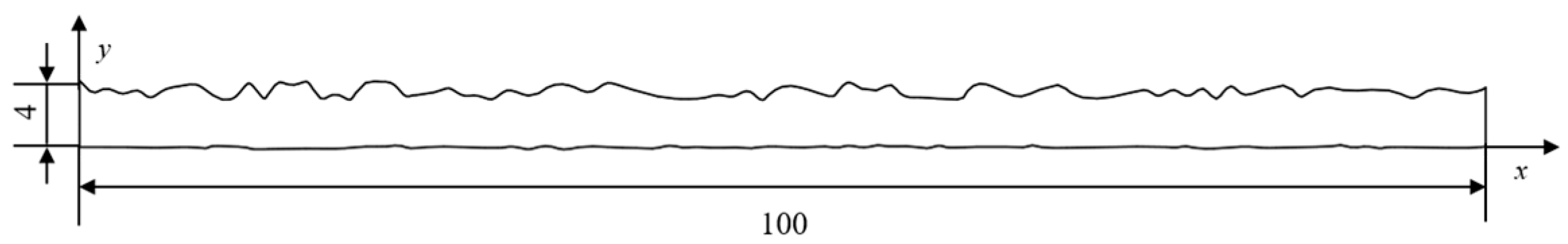
Analyze the relationship between the two-dimensional fractal parameters and the surface contour and morphological complexity, and establish a fit clearance model with a rough surface. Select a part of the fit gap between the spool and the valve sleeve, and establish the calculation model of the rough surface gap, as shown in
Figure 5. The gap length of the calculation model is 100 μm, and the average height of the gap is 4 μm.
The computational results of liquid–solid two-phase flow are affected by the number and quality of meshes. Too many meshes increase the computational cost, while too few meshes do not accurately reflect the flow state, and thus mesh-independence verification is needed. The maximum grid size was adjusted from 8 × 10
−4 mm to 1 × 10
−4 mm, divided into five levels, and the grid-independence was evaluated by analyzing the exit velocity with other boundary conditions being the same. The results are shown in
Table 1.
As can be seen from
Table 1, the exit velocity is largest when the maximum grid size is 8 × 10
−4 mm, and gradually stabilizes at 0.0494 m/s with the refinement of the grid and the increase of the number of grids. The exit velocity of the last three groups does not change much, but the difference in the number of grids is large, which leads to a significant increase in the computation time and cost. Considering the above factors, the minimum grid size of 2 × 10
−4 mm is selected for numerical simulation.
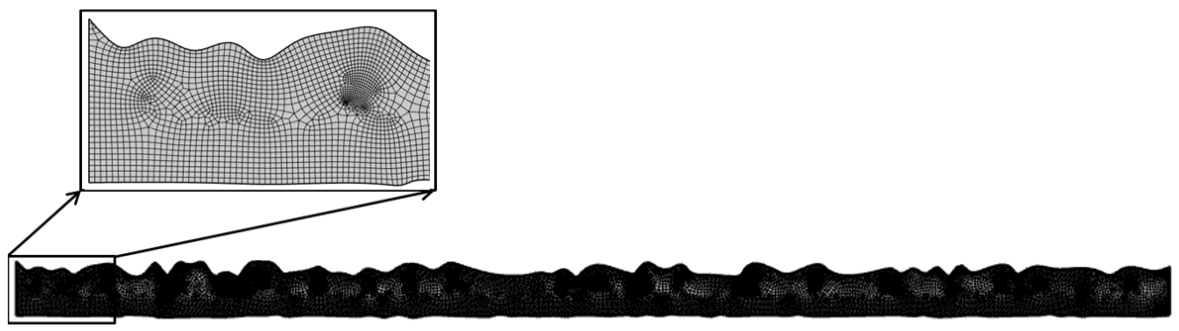
Based on the results of the mesh-independence verification, the maximum mesh size of 2 × 10
−4 mm is set to ensure that the rough flow gap mesh is sufficiently fine, and the final number of meshes generated is 14,813, with an average mesh quality of 0.8914, which meets the requirements of multi-physics field computation. The results of rough gap meshing are shown in
Figure 6.
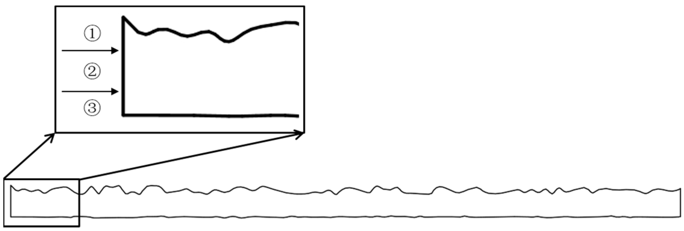
As shown in
Figure 7, the entrance of the computational model is divided into three parts: the first part is the position of releasing particles close to the surface with large roughness (i.e., close to the surface of the valve body), i.e., position ①, with a radial position height of 3–4 μm; the second part is the position of releasing particles in the middle position of the rough flow field model, i.e., position ②, with a radial position height of 1.5–3 μm; and the third part is the position of releasing particles close to the surface with small roughness (i.e., near the surface of the spool), i.e., position ③, with a radial position height of 0 to 1.5 μm.
The computational domain is defined as a fluid domain, with No. 46 antiwear hydraulic oil designated as the fluid medium. The oil has a density of 871 kg/m
3 and a dynamic viscosity of 0.04 Pa-s. The fluid is characterized as incompressible. The boundary conditions are set as velocity inlet and pressure outlet, and the specific parameters are shown in
Table 2.
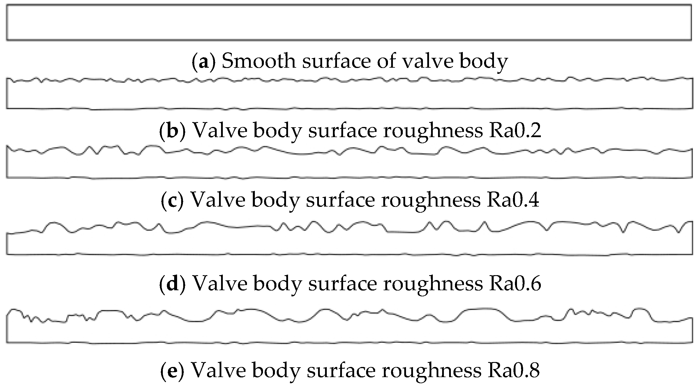
In order to explore the effect of different degrees of roughness of the valve body on the flow field in the mating gap, in this section, through the establishment of different valve body surface roughness calculation model, take the valve body surface smooth, valve body surface roughness Ra0.2, valve body surface roughness Ra0.4, valve body surface roughness Ra0.6, valve body surface roughness Ra0.8—five different degrees of roughness, as shown in
Figure 8—and the rest of the dimensions and the computational conditions remain unchanged. Then, analyze the effect of the rough surface on the gap flow field.
4. Characterization of Particle Transport in a Rough Slide Valve Gap
4.1. Characterization of Particle Motion on Different Rough Surfaces
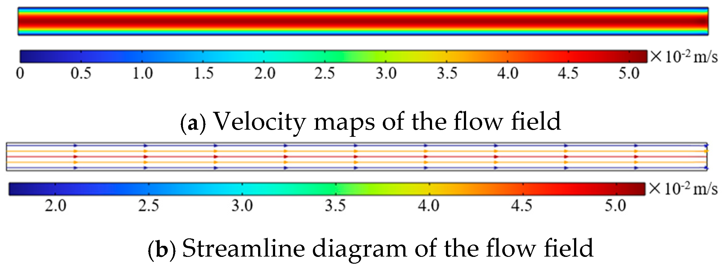
The smooth surface model of the valve body is calculated with an inlet pressure of 0.1 MPa at the inlet port and 0 MPa at the outlet port, and the velocity and pressure clouds of the flow field are obtained as shown in
Figure 9.
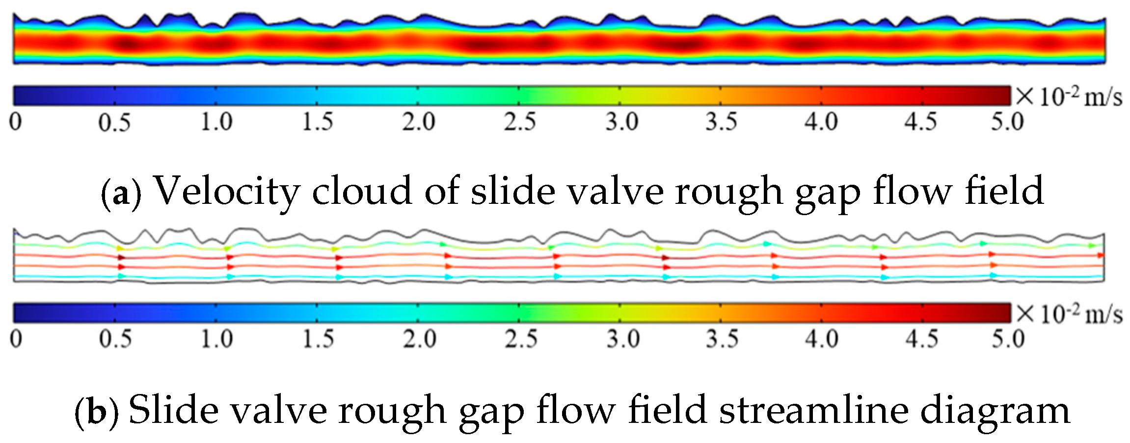
The velocity cloud and streamline diagram of the interstitial flow field at the same boundary condition with the valve body surface roughness Ra0.4 are shown in
Figure 10.
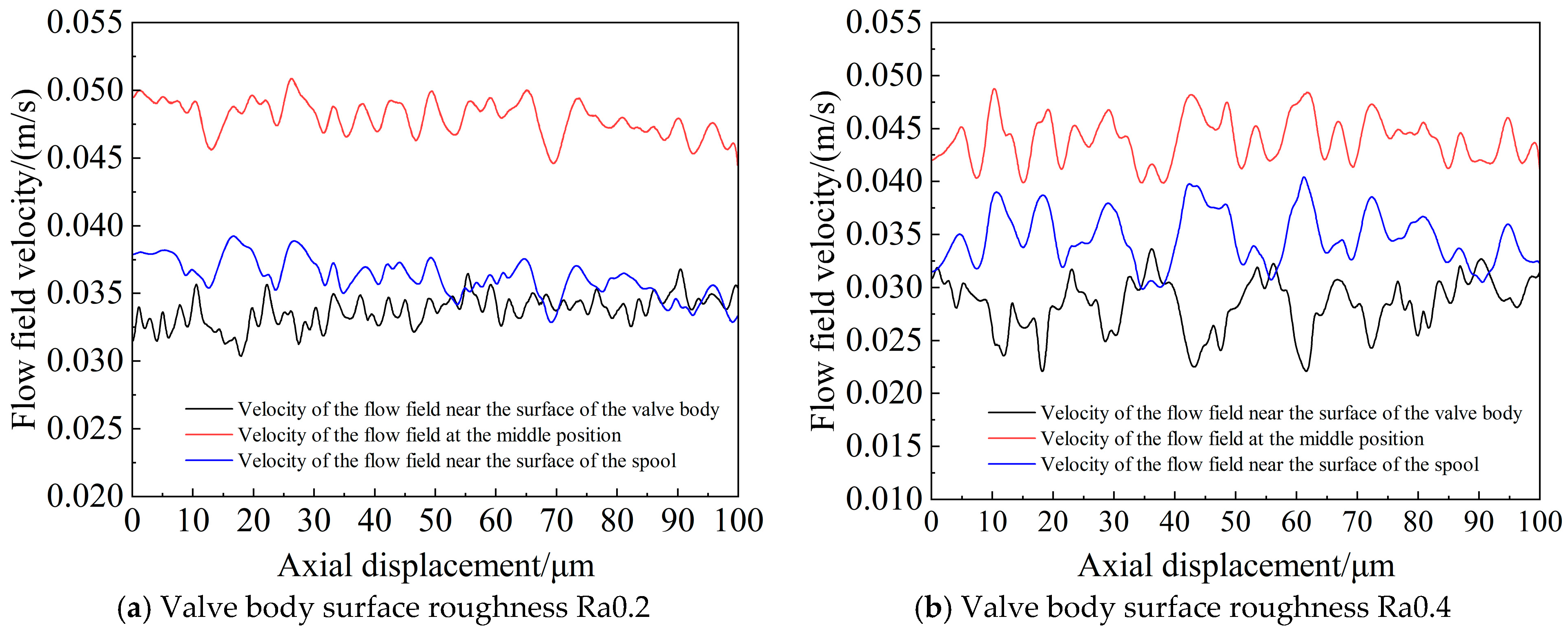
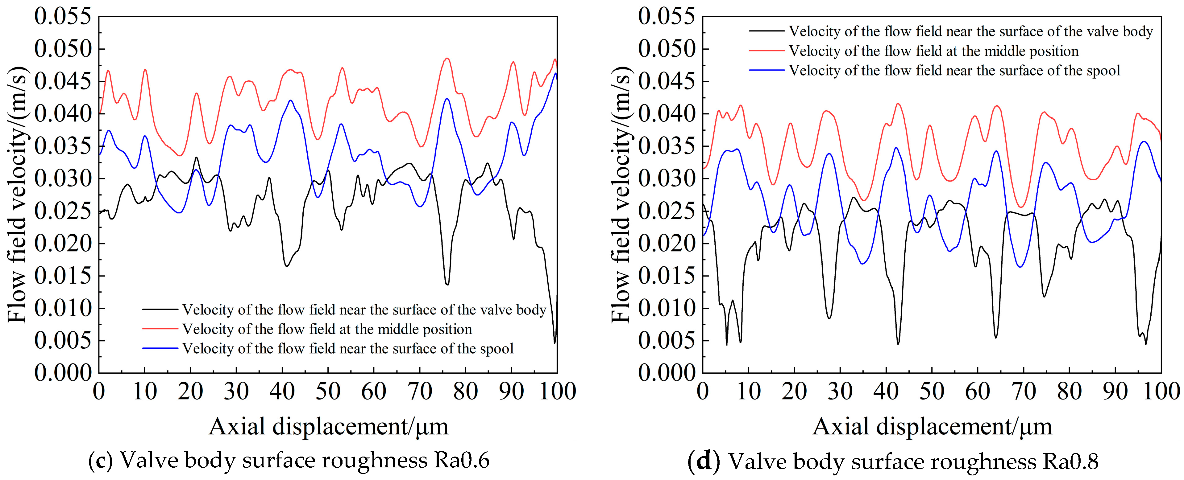
Plots of flow velocity versus axial displacement at three positions in the gap flow field for valve body surface roughness Ra0.2, Ra0.4, Ra0.6, and Ra0.8 are shown in
Figure 11.
As demonstrated in
Figure 11, within the gap-fit flow field, the fluid velocity exhibits a maximum at the intermediate position and a minimum in proximity to the rough surface of the valve body.
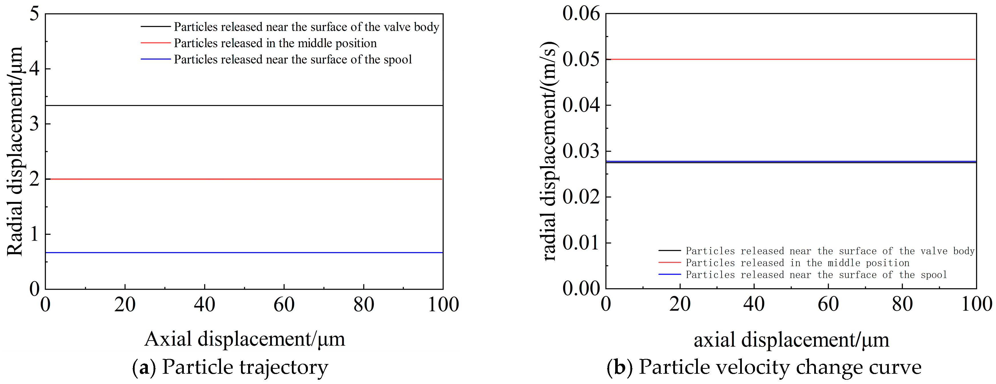
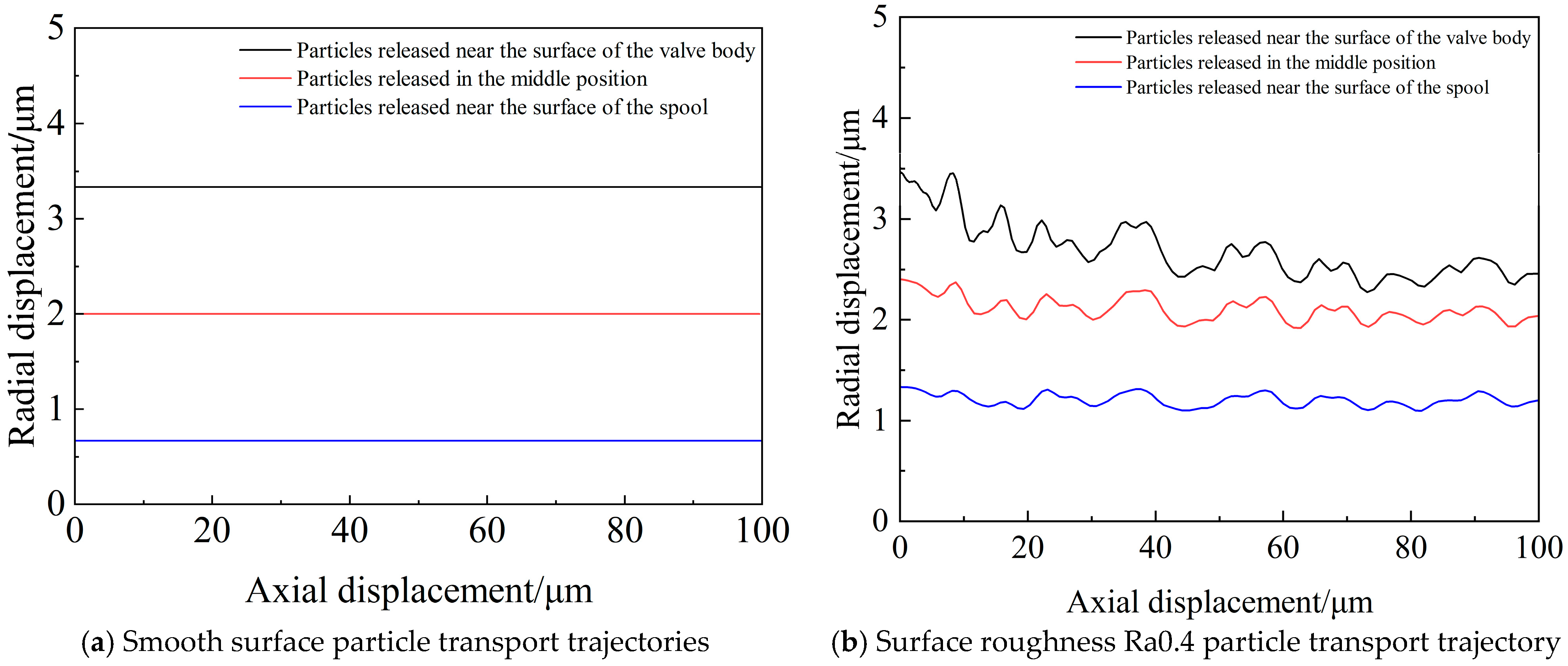
The radial displacements of the particles at the three release positions under the smooth model of the valve body surface are extracted and displayed in
Figure 12.
From
Figure 12, it can be concluded that the spherical ferrous particles in the gap under this calculation condition are driven by the differential pressure flow and enter the gap, and the motion of the particles in the gap in the smooth surface model advances smoothly due to the driving of the flow field.
Since the velocity distribution of the flow field in the smooth gap is stable, the trailing force on the particles in the smooth flow field model is also stable, so the trajectory and velocity of the particles are basically unchanged during the movement in the smooth flow field.
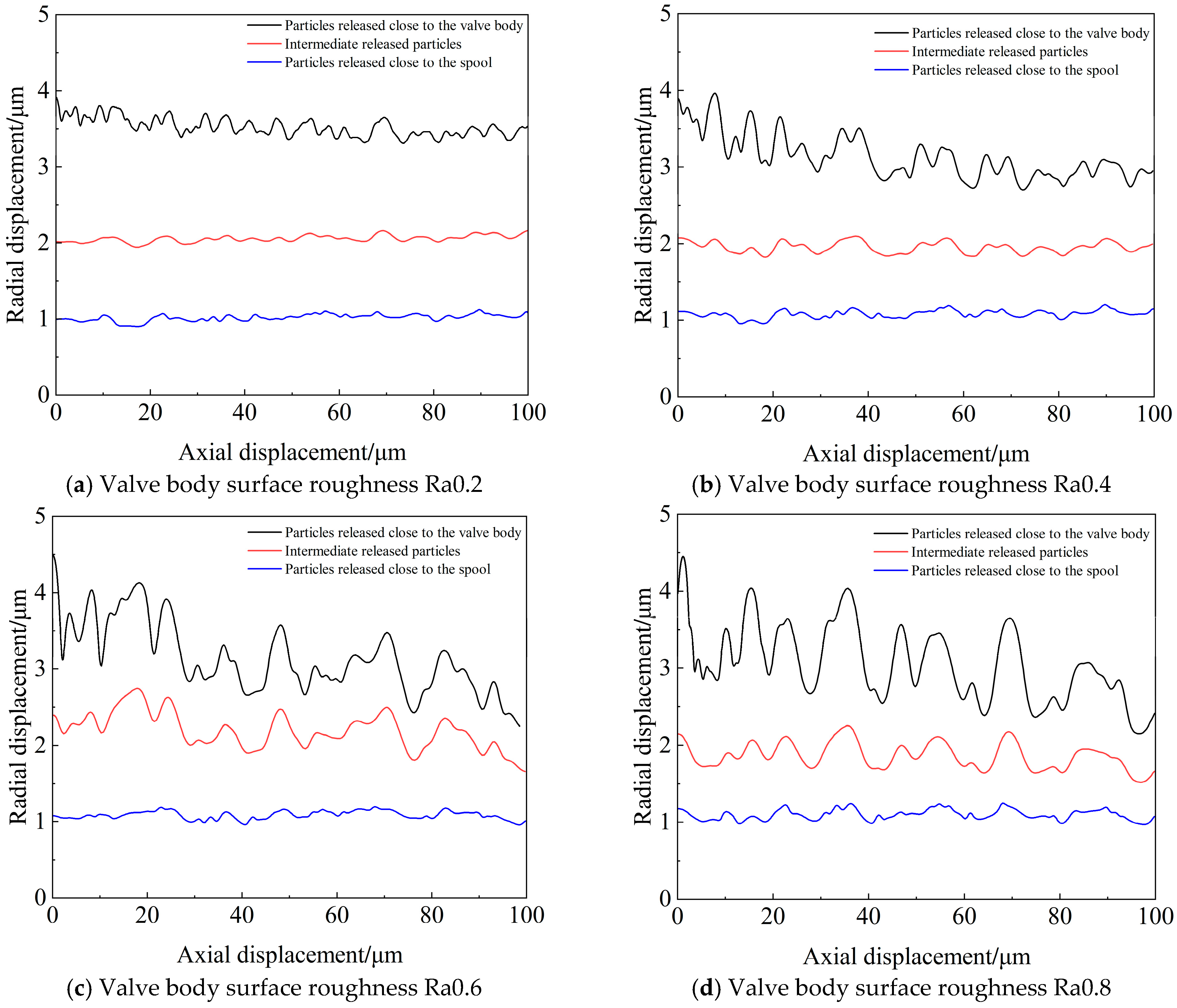
With the increase of the surface roughness of the valve body, the fluctuation of the radial displacement of the particles in the flow field under the three release positions all become more and more violent. Among the three particle release positions, the radial displacement fluctuation of the particles released near the surface of the valve body is the most violent, so the particles released at this position increase the possibility of collision with the wall, increasing the chance of sliding valve stagnation.
As shown in
Figure 13, the irregular structure of rough surfaces leads to velocity fluctuations in the flow field, which affects the radial displacement of particles. Comparing the particle trajectories in
Figure 12a with those in the rough flow field shows that, while the changes in radial displacement and velocity of particles released from the smooth surface are relatively smooth, those in the rough flow field fluctuate more. As the roughness of the valve surface increases, the fluctuations in radial displacement of particles released from all three positions become more intense. Of the three particle release positions, those close to the valve body surface experience the most violent fluctuations in radial displacement, increasing the likelihood of collision with the wall and the chance of sliding valve stagnation.
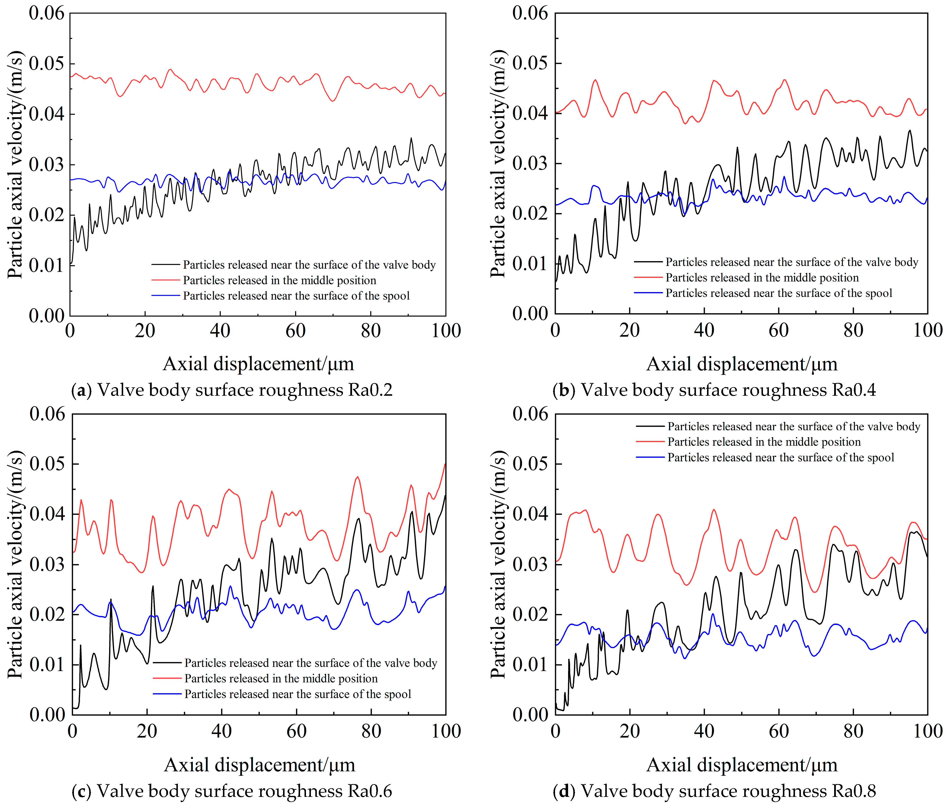
The curves of particle motion velocity versus displacement for the three types of particle release locations under different rough surface models are shown in
Figure 14. From
Figure 14, it can be seen that the particles are driven by the flow field, and the motion velocity of the particles is also the largest in the middle position, where the flow field velocity is large, and the motion velocities of the particles released in the other two positions are all smaller than that of the particles released in the middle position because of the smaller velocity of the flow field in which they are located.
4.2. Characterization of Particle Motion in Flow Fields with Different Flow Velocities
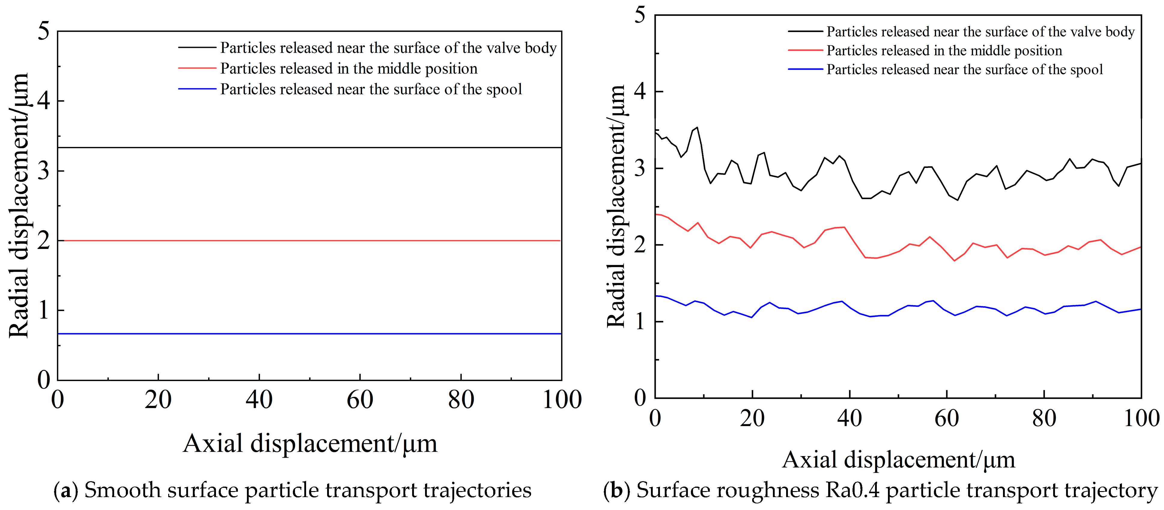
In order to investigate the motion characteristics of micron particles in the sliding valve gap under different flow velocities, two cases of valve body surface smooth and valve body surface roughness Ra0.4 were selected to analyze the motion characteristics of particles under different fluid motion velocities at different release positions and different roughness surfaces with inlet velocities of 20 m/s and 120 m/s, for example, as shown in
Figure 15 and
Figure 16.
According to
Figure 15 and
Figure 16, the particle transport trajectories for different flow rates at the same surface roughness and the same particle release position are basically the same for 20 m/s and 120 m/s flow rates, and the change of flow rate does not affect the change of particle transport trajectories in the flow field.
5. Particle Transport Results Processing
5.1. Characterization of Particulate Matter Transport Under Different Conditions
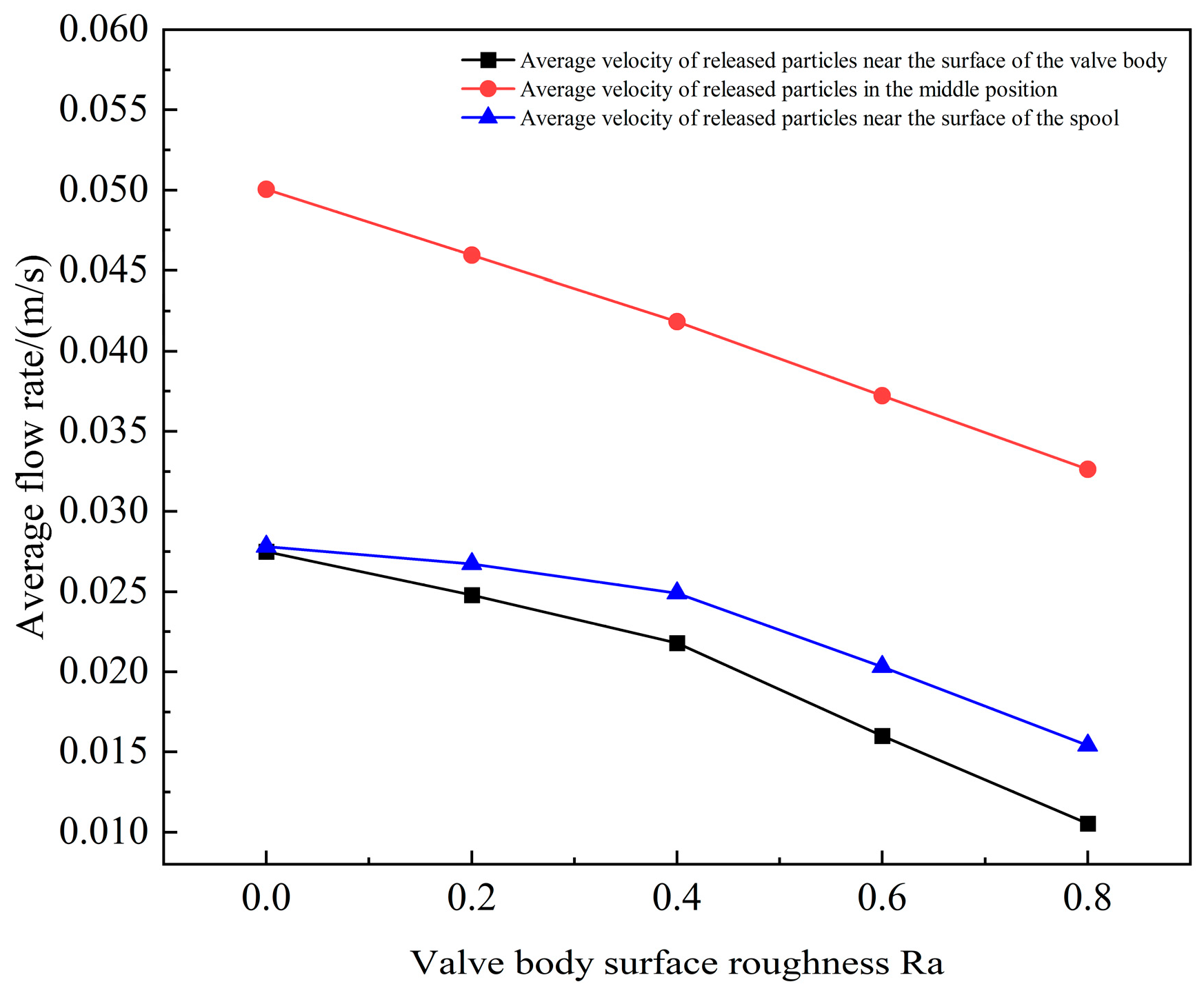
Figure 17 shows the average velocity profiles of particles under different degrees of roughness of the valve body surface and three release positions (near the valve body surface, in the middle position, and near the valve spool). The analysis shows that the particle flow velocity decreases with the increase of surface roughness, and there are differences in the particle flow velocities at different positions: the particle flow velocity is the lowest near the surface of the valve body and the highest at the middle position.
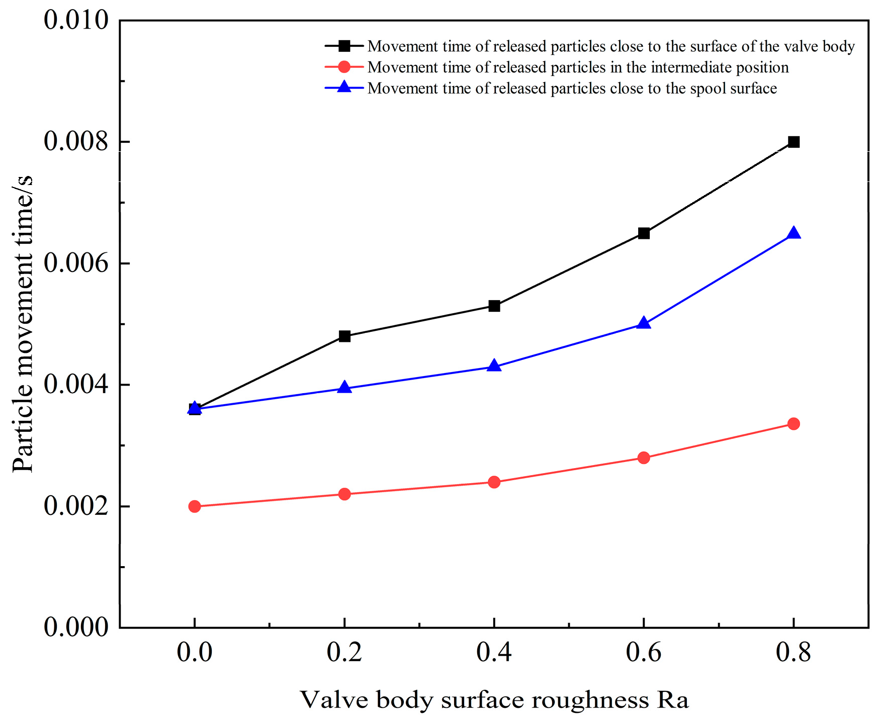
Figure 18 presents the motion time of the three types of particles within the rough gap flow field. The results show that the particle motion time increases significantly with the increase of surface roughness, and there are differences in the particle motion time at different locations, with the longest particle motion time near the surface of the valve body and the shortest at the middle location. The rough surface increases the radial displacement of the particles, prolongs the transportation time, and raises the risk of stalling. From
Figure 18, a trend can be seen: when the valve body surface roughness Ra in 0.4 before, the movement time growth is flat; more than Ra0.4, the growth is obviously accelerated. That is, when Ra < 0.4, the roughness increase has a small effect on the particle transportation time; when Ra ≥ 0.4, the roughness increase significantly increases the particle transportation time. Therefore, Ra0.4 can be taken as the roughness cut-off point. This is because the increase in roughness increases the number of raised structures on the surface, and the number and chance of collision between the particles near the surface of the valve body and these structures increase, thus prolonging the transport time. In summary, in order to reduce the transport time of particles in the rough gap, reduce the slide valve stall phenomenon, while taking into account the processing accuracy and cost, it is recommended that the valve body surface roughness control in Ra0.4 below.
Under different flow rates, the transportation time of particles released from different surface roughness and different positions is shown in
Figure 19. According to
Figure 19, it can be concluded that the particle transport trajectory in the flow field of the slide valve gap is only related to the surface roughness of the valve body, and different velocities will not lead to a large difference in the particle trajectory. The faster the inlet velocity, the shorter the particle transport time.
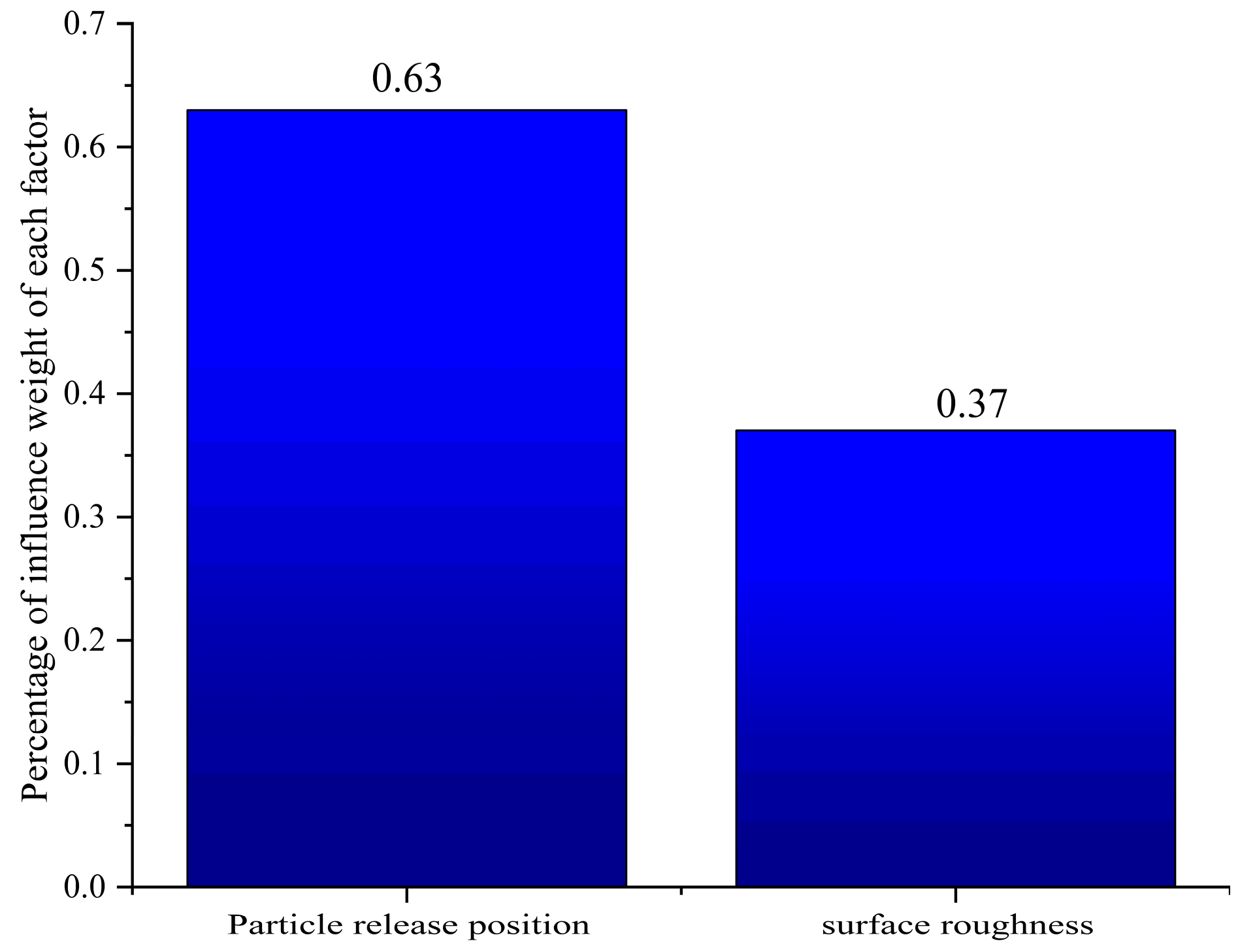
5.2. Weighting of Factors Influencing Particle Transport
In order to analyze the influence weights of these factors on the particle motion time, multiple linear regression methods were used to reveal the relationship between the variables by fitting the data model. This time, a large amount of simulation data was used, which included the particle motion time under different independent variable conditions, and after standardization, the standardized regression coefficients were calculated by using the regression analysis method, and the weights of the independent variables were normalized to obtain the influence weights of each factor on the particle motion time.
Figure 20 shows the normalized weight results. The influence of particle release position on particle movement time accounts for 63% of the weight, while the effect of valve body surface roughness on particle movement time accounts for 37%.
6. Experimental Research
6.1. Experimental Model Similarity Calculations
Since both the actual model and the simulation model are in micrometer scale, directly using the actual model for processing and experimental analysis will greatly increase the difficulty of analysis. Therefore, in order to ensure the feasibility and accuracy of the experiments, it is necessary to use appropriate similarity theory to enlarge the actual model. In the design of the experimental model, the model is first enlarged by 500 times through geometric similarity, and the micrometer scale is converted to millimeter scale. In order to ensure the consistency of the flow field and the motion characteristics of the particles in different scales, the Reynolds number similarity is utilized to make the model have the same flow characteristics before and after the enlargement; meanwhile, the Stokes number similarity is utilized to ensure the consistency of the motion characteristics of the particles in the two models.
Reynolds number is an important dimensionless number in fluid dynamics, which describes the ratio of inertial force to viscous force of the flow. When calculating the flow velocity of the enlarged model, in order to maintain the similarity of Reynolds number, it should be ensured that the Reynolds number of the original model and the enlarged model are equal, which is given in the following equation:
where
—Fluid density (kg/m
3);
—model boundary dimensions (m);
—average velocity of flow field (m/s);
—dynamic viscosity (Pa-s);
—simulated flow field;
—experimental flow field.
In this experiment, No. 46 antiwear hydraulic oil is used, with a density of 871 kg/m
3 and a viscosity of 0.04 Pa-s. Due to the opacity of the hydraulic oil and the possible leakage problem, water is chosen as the experimental medium. The density of water at 20 °C is 1000 kg/m
3, and the viscosity is 1.005 × 10
−3 Pa-s. The boundary size of the experimental model is 500 times that of the simulation model, and the flow rate of the experimental model is calculated according to the formula that follows:
To ensure the feasibility of the flow velocity in the experiment, the inlet velocity in the simulated flow field was selected to be 120 m/s. After calculation, the inlet velocity of the experimental model was 0.005226 m/s. The inlet was a circular port with an outer diameter of 8 mm and an inner diameter of 6 mm, and the inlet flow rate was 0.0089 L/min.
In the interstitial flow field, particles are mainly affected by the trailing force of the flow field. To ensure that the particles have similar dynamics in experimental and simulation models, the motion of the particles should satisfy similar mechanical laws. The Stokes number is used to characterize the motion of the particles in the fluid, especially the ratio of the inertial force to the viscous force of the particles. To ensure the similarity of particle motion, the Stokes number of the model before and after enlargement should be consistent. The Stokes number is calculated as
where
—particle density (kg/m
3);
—model boundary dimensions (m);
—particle diameter (m);
—average fluid velocity (m/s);
—fluid power viscosity (Pa-s);
—simulation model;
—experimental model.
In order to observe the trajectory of the particles in the flow field, particles with a diameter of 1 mm were selected for the experiment. According to the Stokes number similarity calculation, the density of the experimental particles is 2264.42 kg/m3, so an aluminum alloy whose density is 2300 kg/m3 was chosen as the particle material, and the particle diameter was 1 mm.
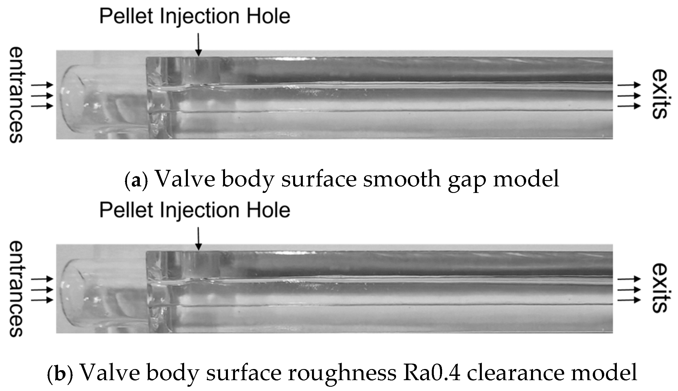
6.2. Experimental Model
The experimental model was fabricated using 3D printing, with the rough surface of the simulation model scaled up proportionally. To ensure optimal imaging quality, a transparent material with high light transmittance was used for printing. After printing, the internal flow field of the model was polished to minimize the impact of processing accuracy and material properties on the experimental results. Based on these requirements, two simulation models—one with a smooth valve body surface and the other with a valve body surface roughness of Ra0.4—were processed to obtain the experimental model, as shown in
Figure 21.
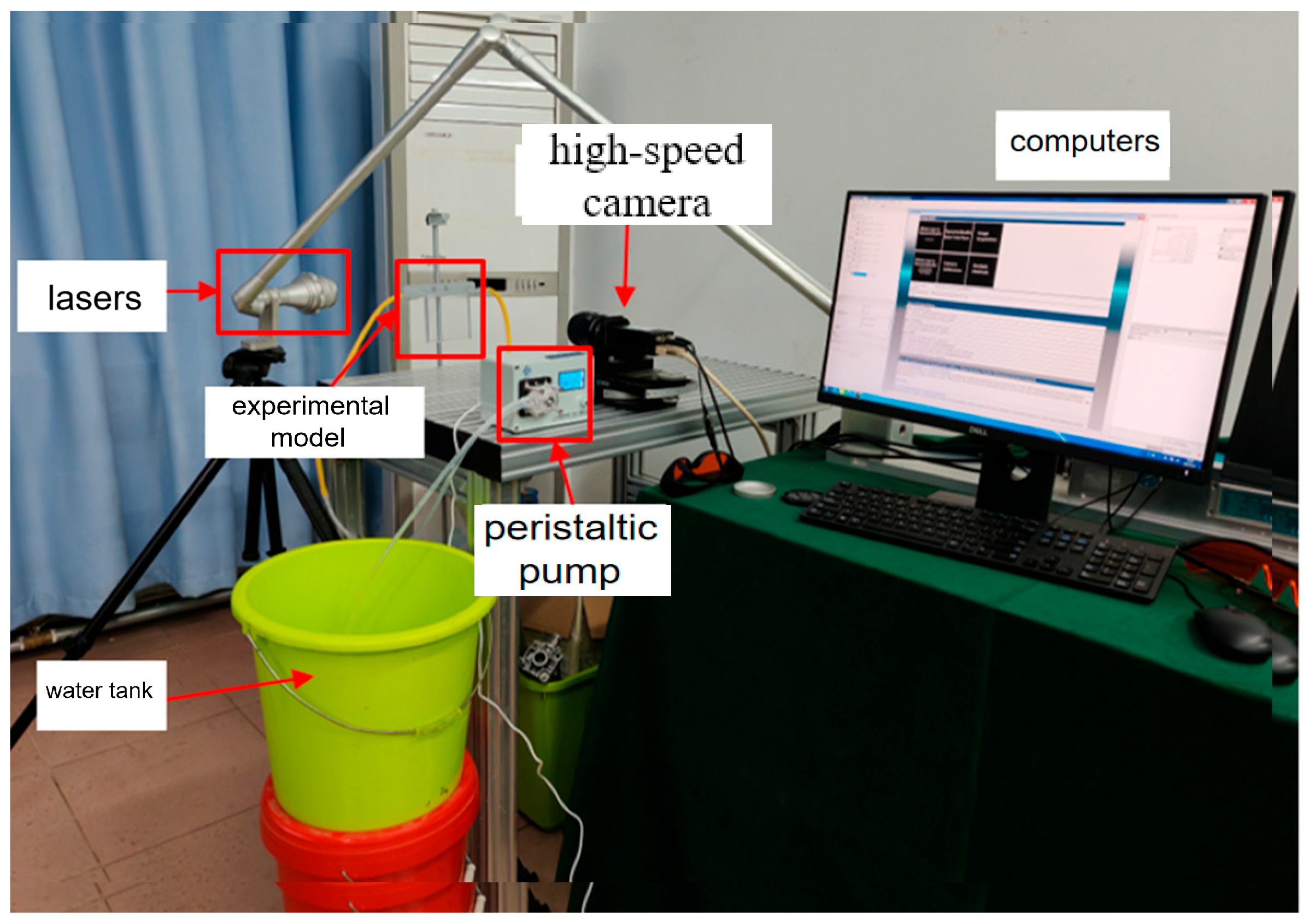
The experimental setup included a laser, a high-speed camera, a computer, and a fluid flow system. Before the experiment began, it was essential to ensure the precise alignment of the laser and the high-speed camera, with the laser’s illuminated plane matching the imaging plane of the camera. To calibrate the system, suitable tracer particles were selected and evenly distributed, ensuring that particle movement in the flow field could be accurately captured. Image processing algorithms were used to analyze the particle positions, calculate the velocity distribution, and correct any errors. Zero-point calibration was performed before the experiment by setting up a stationary fluid to eliminate system biases, ensuring the accuracy of the measurements. The liquid flow rate was adjusted using a precisely controlled peristaltic pump and verified using a flow meter to ensure the stability of the flow rate during the experiment. Environmental factors such as temperature, humidity, and vibrations were strictly controlled to minimize interference with the experimental data. To further enhance the reliability of the experiment, a detailed inspection of the equipment was carried out before each experiment, including checking the laser spot, cleaning the camera lens, and confirming the functionality of the flow control system. Additionally, the system was periodically calibrated during the experiment and compared with theoretical models to ensure data accuracy and consistency. To maintain long-term experimental precision, the equipment required regular maintenance and calibration, with recalibration performed before and after each experiment to eliminate potential system drift, ensuring high reliability of the experimental results. The lab bench is shown in
Figure 22.
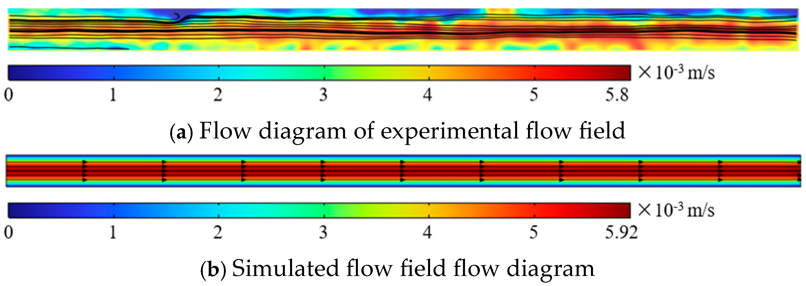
6.3. Enlarged Gap Model Flow Field Characterization
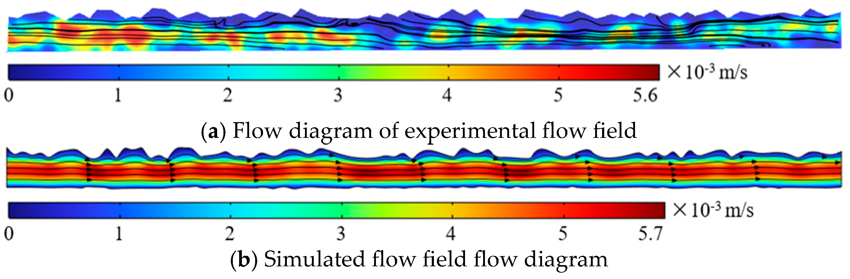
Through the PIV experiment, the velocity cloud and streamline distribution of the smooth gap flow field and the valve body surface roughness Ra0.4 gap flow field were obtained, compared, and analyzed with the simulation results, as shown in
Figure 23 and
Figure 24. After similar theoretical amplification of the model and the original model, the flow trend was basically the same; the rough surface of the flow field of the influence of the law and the simulation results were consistent with the simulation results, to verify the previous simulation method and the correctness of the simulation results.
6.4. Particle Transport Law in the Enlarged Gap Model
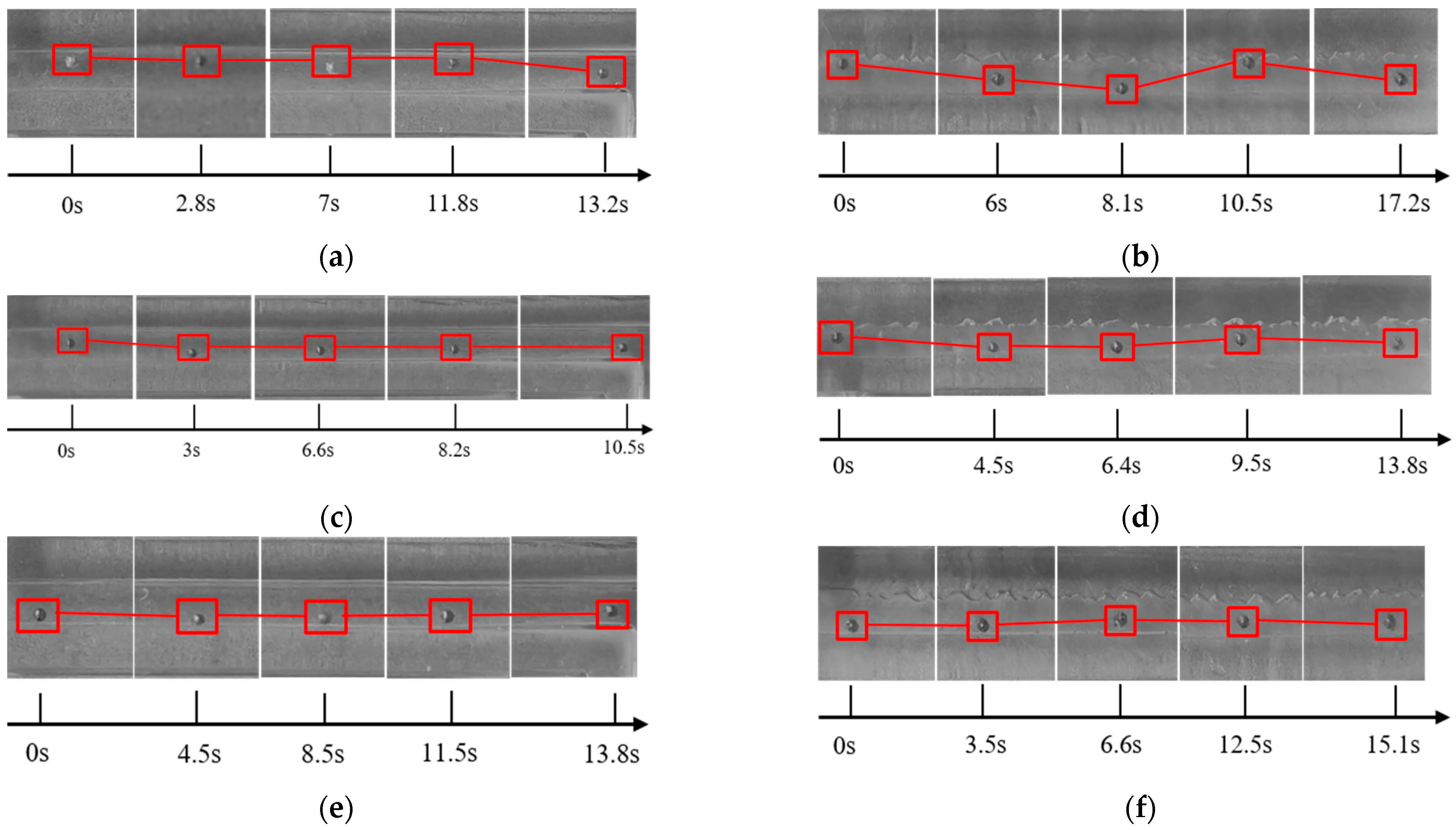
The particles were injected into the flow field from the particle injection holes reserved in the model using the particle injection device. By moving the position of the particle injection device, the release of particles at different positions in the flow field was realized, and after the particles were released, the peristaltic pump was turned on according to the experimental boundary conditions, and a camera was utilized to record the motion of the particles in the interstitial flow field. The experimental results are shown in
Figure 25.
Based on the experimental results, it can be concluded that in the experimental models with different rough surfaces, the flow velocity in the middle position of the flow field is the fastest, so the particles released in the middle position have the shortest movement time. For particles released at the same position in different experimental models, the average flow velocity within the rough model is less than the average flow velocity within the smooth model due to the presence of rough surfaces in the rough flow field model, and therefore the transport time of particles in the rough model is longer than that in the smooth model.
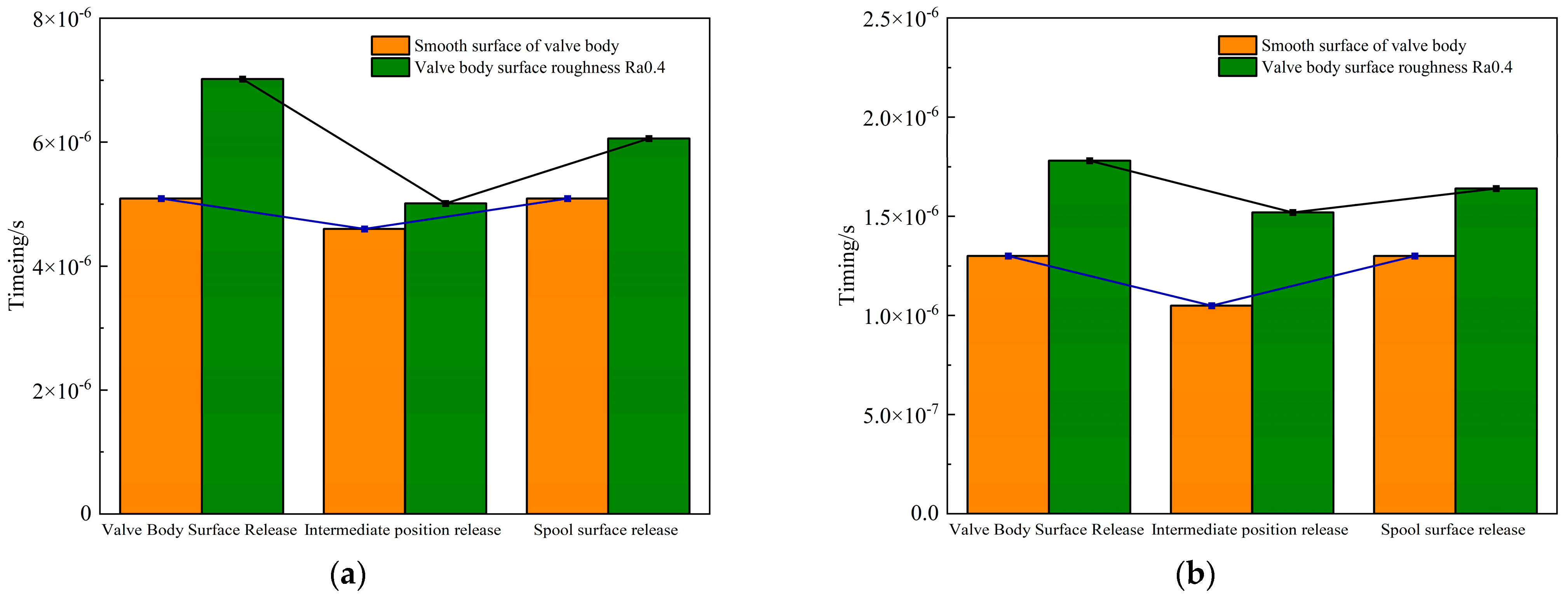
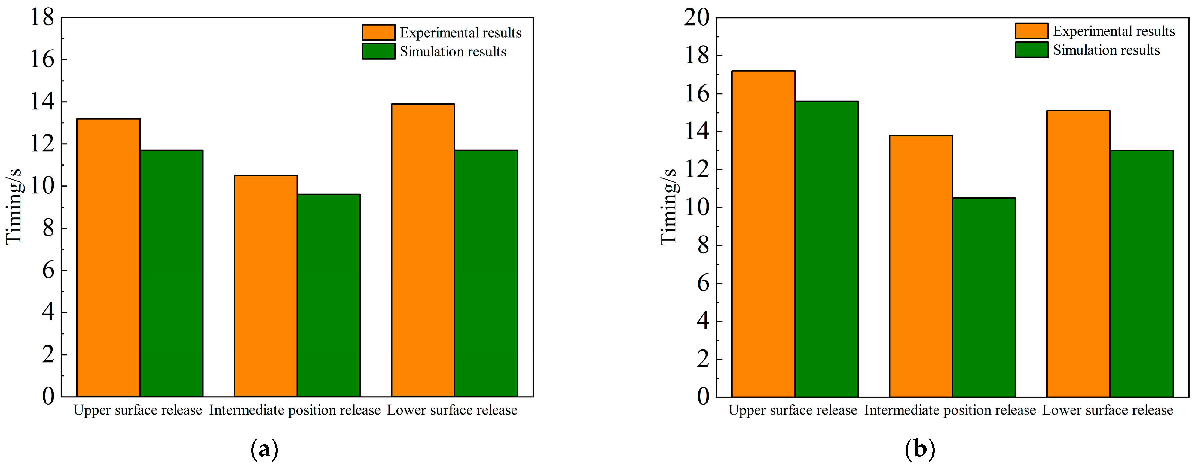
The transport of particles in the enlarged slide valve gap model is computationally analyzed, the computational setup method and the particle force setup are consistent with the previous paper, and the computational boundary conditions are consistent with the experimental conditions. The experimental and simulation results of the particle transport time under the same release position in the same model are obtained as shown in
Figure 26.
By using the same calculation and analysis method for the enlarged model, the particle transport law in the rough gap model is consistent with that in the previous paper, and the comparison of the experimental results shows that the calculation and analysis method has an accuracy of 85%, so it can be concluded that the liquid–solid two-phase flow calculation model used in the previous paper has a certain degree of accuracy.
7. Conclusions
In this study, a series of spool valve gap models with varying surface roughness were established based on fractal theory to more accurately represent non-ideal contact surfaces in real engineering systems. A coupled liquid–solid two-phase flow model and scaled-up experimental validation were used to systematically analyze the influence of wall roughness and particle release position on transport behavior. The main conclusions are as follows:
- 1.
A fractal-based modeling method for rough valve gaps was established
This approach overcomes the common assumption of idealized smooth contact surfaces in previous studies and more realistically captures the effects of surface roughness on flow and particle behavior under practical conditions.
- 2.
The impact of surface roughness on flow field structure and particle transport was clarified
Increasing surface roughness led to stronger flow disturbances and local vortex formations, causing more pronounced trajectory fluctuations and longer migration paths.
Particles released near the rough wall exhibited the longest transport times. A critical threshold was identified at Ra = 0.4, above which the migration time increased significantly; below this value, the increase was moderate. For instance, in the Ra = 0.6 model, the average migration time increased by approximately 41.2% compared to the ideal smooth-wall model.
- 3.
Particle trajectories are insensitive to flow velocity changes
Under two high-flow velocity conditions, the particle paths remained nearly identical, indicating that in laminar regimes, boundary-induced effects dominate particle behavior rather than fluid inertia.
Flow rate only affected the overall migration time, not the trajectory pattern.
- 4.
The particle release position plays a dominant role in transport behavior
Differences in initial release positions lead to variations in wall proximity, local shear forces, and flow fluctuations, which directly affect particle migration time and path characteristics.
- 5.
Multiple linear regression was used to quantify the relative influence of key factors
The analysis revealed that the release position contributes 63% to the variation in particle migration time, while surface roughness accounts for 37%.
This highlights the dominant role of initial boundary conditions in determining particle transport characteristics.
- 6.
The study provides important engineering value and practical significance
Most existing studies assume idealized surface geometries, which fail to capture the real effects of roughness on transport performance.
This research reveals the mesoscopic coupling mechanisms between wall roughness, release position, and particle behavior, bridging the gap between ideal assumptions and real-world performance.
The findings offer theoretical support and design references for improving the anti-jamming reliability and contamination tolerance of fuel electro-hydraulic servo valves, with important implications for enhancing the reliability of aerospace hydraulic systems.
8. Future Work
Future research will focus on the following aspects:
To better reflect real-world contamination scenarios, future studies will consider particles of varying sizes and material properties. This will allow for a more comprehensive understanding of particle–flow–wall interactions within rough valve gaps.
- 2.
Refining the model through deeper quantitative analysis
Further efforts will be made to enhance the model accuracy by integrating more extensive simulation data, experimental validation, and parameter sensitivity studies. Multiscale modeling techniques may also be introduced to capture behaviors across different spatial resolutions.
- 3.
Extending model applicability to diverse operating conditions
The current framework will be adapted for different working fluids, temperature ranges, and flow regimes to assess its robustness under various real-world aerospace and industrial scenarios.
- 4.
Promoting engineering integration and practical implementation
By collaborating with hydraulic system manufacturers, the model can be embedded into the design and reliability assessment process of electro-hydraulic servo valves, thus supporting the development of next-generation, high-reliability components.
Author Contributions
Methodology, J.Z. and R.D.; software, K.Z. (Kuo Zhang) and R.D.; validation, J.Z. and R.D.; data curation, K.Z. (Kuohang Zhang); resources, P.D., S.W. and Y.L.; formal analysis, R.D.; writing—original draft preparation, R.D., P.D. and K.Z. (Kuohang Zhang); writing—review and editing, J.Z., R.D., P.D. and K.Z. (Kuohang Zhang). All authors have read and agreed to the published version of the manuscript.
Funding
This research was funded by the National Natural Science Foundation of China, grant number 52275068. This research was funded by the Open Foundation of the State Key Laboratory of Taihang Laboratory, grant number QTJLHT202404090002.
Data Availability Statement
Data are contained within the article.
Acknowledgments
This research would like to thank Hangzhou Applied Acoustics Research Institute and AVIC Changchun Control Technology for their technical support.
Conflicts of Interest
Author Shengrong Wang was employed by the company AVIC Changchun Control Technology. Pengpeng Dong was employed by the company Hangzhou Applied Acoustics Research Institute. The remaining authors declare that the research was conducted in the absence of any commercial or financial relationships that could be construed as a potential conflict of interest.
References
- Jiao, Z.X.; Wu, S.; Li, Y.; Zhang, C.; Jin, H.T.; Shu, S.; Wei, R.L.; Li, R.J.; Wang, Y.; Zhang, H.Y.; et al. Development Status and Trends of the Intelligence of Hydraulic Components and Systems. J. Mech. Eng. 2023, 59, 357–384. [Google Scholar]
- Gürbüz, H. Optimization of combustion and performance parameters by intake-charge conditions in a small-scale air-cooled hydrogen fuelled SI engine suitable for use in piston-prop aircraft. Aircr. Eng. Aerosp. Technol. 2021, 93, 448–456. [Google Scholar] [CrossRef]
- Lindler, J.E.; Anderson, E.H. Piezoelectric direct drive servovalve. In Smart Structures and Materials 2002: Industrial and Commercial Applications of Smart Structures Technologies, Proceedings of the SPIE's 9th Annual International Symposium on Smart Structures and Materials, San Diego, CA, USA, 17–21 March 2002; SPIE Digital Library: Washington, DC, USA; pp. 488–496.
- Liu, X.Q.; Liu, F.; Ji, H.; Li, N.; Wang, C.; Lin, G. Particle erosion transient process visualization and influencing factors of the hydraulic servo spool valve orifice. Flow Meas. Instrum. 2023, 89, 102273. [Google Scholar] [CrossRef]
- Liu, X.; Ji, H.; Liu, F.; Li, N.; Zhang, J.; Ren, W. Particle motion and erosion morphology of the spool orifice in an electrohydraulic servo valve under a small opening. Proc. Inst. Mech. Eng. Part. C J. Mech. Eng. Sci. 2022, 236, 3160–3173. [Google Scholar] [CrossRef]
- Singh, M.; Lathkar, G.S.; Basu, S.K. Failure prevention of hydraulic system based on oil contamination. J. Inst. Eng. Ser. C. 2012, 93, 269–274. [Google Scholar] [CrossRef]
- Zhang, H.P.; Huang, W.; Zhang, Y.D.; Shen, Y.; Li, D.Q. Design of the microfluidic chip of oil detection. Appl. Mech. Mater. 2012, 117, 517–520. [Google Scholar]
- Peng, W.; Cao, X.; Ma, L.; Wang, P.; Bian, J.; Lin, C. Sand erosion prediction models for two-phase flow pipe bends and their application in gas-liquid-solid multiphase flow erosion. Powder Technol. 2023, 421, 118421. [Google Scholar] [CrossRef]
- Xie, Z.; Wang, S.; Shen, Y. CFD-DEM modelling of the migration of fines in suspension flow through a solid packed bed. Chem. Eng. Sci. 2021, 231, 116261. [Google Scholar] [CrossRef]
- Wang, X.; Gong, L.; Li, Y.; Yao, J. Developments and applications of the CFD-DEM method in particle–fluid numerical simulation in petroleum engineering: A review. Appl. Therm. Eng. 2023, 222, 119865. [Google Scholar] [CrossRef]
- Yang, Z.; Lian, X.; Savari, C.; Barigou, M. Evaluating the effectiveness of CFD-DEM and SPH-DEM for complex pipe flow simulations with and without particles. Chem. Eng. Sci. 2024, 288, 119788. [Google Scholar] [CrossRef]
- Ranjbari, P.; Emamzadeh, M.; Mohseni, A. Numerical analysis of particle injection effect on gas-liquid two-phase flow in horizontal pipelines using coupled MPPIC-VOF method. Adv. Powder Technol. 2023, 34, 104235. [Google Scholar] [CrossRef]
- Shokri, R.; Ghaemi, S.; Nobes, D.S.; Sanders, R.S. Investigation of particle-laden turbulent pipe flow at high-Reynolds-number using particle image/tracking velocimetry (PIV/PTV). Int. J. Multiph. Flow 2017, 89, 136–149. [Google Scholar] [CrossRef]
- Thaker, H.A.; Karthik, G.; Buwav, V. PIV measurements and CFD simulations of the particlescale flow distribution in a packed bed. Chem. Eng. J. 2019, 374, 189–200. [Google Scholar] [CrossRef]
- Mittal, R.; Iaccarino, G. Immersed boundary methods. Annu. Rev. Fluid Mech. 2005, 37, 239–261. [Google Scholar] [CrossRef]
- Terrelle, J.; Higgs, C.F. A modeling approach for predicting the abrasive particle motion during chemical mechanical polishing. J. Tribol. 2007, 129, 933–941. [Google Scholar] [CrossRef]
- Tic, V.; Lovrec, D. Trajectories of solid and gaseous particles in a hydraulic reservoir. In Proceedings of the 8th International Fluid Power Conference IFK, Dresden, Germany, 26–28 March 2012. [Google Scholar]
- Yohsuke, T.; Gen, O.; Yoshimichi, H. Experimental study on the interaction between large scale vortices and particles in liquid-solid two-phase flow. Int. J. Multiph. Flow 2003, 29, 361–373. [Google Scholar]
Figure 1.
Schematic diagram of internal structure of fuel electro-hydraulic servo valve.
Figure 1.
Schematic diagram of internal structure of fuel electro-hydraulic servo valve.
Figure 2.
Force on sensitive particles in the interstitial flow field.
Figure 2.
Force on sensitive particles in the interstitial flow field.
Figure 3.
Fractal curves of W-M functions for different fractal dimensions D.
Figure 3.
Fractal curves of W-M functions for different fractal dimensions D.
Figure 4.
W-M fractals of surface profile curves with different characteristic scale parameters G.
Figure 4.
W-M fractals of surface profile curves with different characteristic scale parameters G.
Figure 5.
Rough gap calculation model.
Figure 5.
Rough gap calculation model.
Figure 6.
Rough gap calculation model meshing.
Figure 6.
Rough gap calculation model meshing.
Figure 7.
Classification of different particle inlet positions.
Figure 7.
Classification of different particle inlet positions.
Figure 8.
Modeling of different rough surfaces.
Figure 8.
Modeling of different rough surfaces.
Figure 9.
Smooth gap flow field calculations.
Figure 9.
Smooth gap flow field calculations.
Figure 10.
Surface roughness Ra0.4 rough gap flow field calculation results.
Figure 10.
Surface roughness Ra0.4 rough gap flow field calculation results.
Figure 11.
Flow velocity at each position of gap flow field model with different surface roughness.
Figure 11.
Flow velocity at each position of gap flow field model with different surface roughness.
Figure 12.
Calculated results for particles in the smooth gap flow field.
Figure 12.
Calculated results for particles in the smooth gap flow field.
Figure 13.
Particle transport trajectories at different roughness levels.
Figure 13.
Particle transport trajectories at different roughness levels.
Figure 14.
Particle transport velocity at different roughness.
Figure 14.
Particle transport velocity at different roughness.
Figure 15.
Particle transport trajectories under different surfaces at a flow rate of 20 m/s.
Figure 15.
Particle transport trajectories under different surfaces at a flow rate of 20 m/s.
Figure 16.
Particle transport trajectories under different surfaces at a flow rate of 120 m/s.
Figure 16.
Particle transport trajectories under different surfaces at a flow rate of 120 m/s.
Figure 17.
Average velocity of particle transport at different degrees of roughness.
Figure 17.
Average velocity of particle transport at different degrees of roughness.
Figure 18.
Particle transport time for different surface roughness.
Figure 18.
Particle transport time for different surface roughness.
Figure 19.
Particle transport time at different inlet velocities. (a) Particle transport time at different positions at an inlet velocity of 20 m/s. (b) Particle transport time at different positions at an inlet velocity of 120 m/s.
Figure 19.
Particle transport time at different inlet velocities. (a) Particle transport time at different positions at an inlet velocity of 20 m/s. (b) Particle transport time at different positions at an inlet velocity of 120 m/s.
Figure 20.
Weighting of the effect of different factors on the movement time of particles.
Figure 20.
Weighting of the effect of different factors on the movement time of particles.
Figure 21.
Visualization of experimental models for enlarging the gap.
Figure 21.
Visualization of experimental models for enlarging the gap.
Figure 22.
High-speed visualization test bench for slide valve gap flow field.
Figure 22.
High-speed visualization test bench for slide valve gap flow field.
Figure 23.
Experimental and simulation results of surface smooth gap modeling.
Figure 23.
Experimental and simulation results of surface smooth gap modeling.
Figure 24.
Surface roughness Ra0.4 gap model experimental and simulation results.
Figure 24.
Surface roughness Ra0.4 gap model experimental and simulation results.
Figure 25.
Particle transport trajectories and timing. (a) Smooth model top position particles. (b) Valve body surface roughness Ra0.4 model above position particles. (c) Smooth model center position particles. (d) Valve body surface roughness Ra0.4 model center position particles. (e) Smooth model underneath position particles. (f) Valve body surface roughness Ra0.4 model below position particles.
Figure 26.
Experimental and simulation results on particle transport time. (a) Particle transport time in the smooth gap model. (b) Surface roughness Ra0.4 particle transport time in gap models.
Figure 26.
Experimental and simulation results on particle transport time. (a) Particle transport time in the smooth gap model. (b) Surface roughness Ra0.4 particle transport time in gap models.
Table 1.
Comparison of export speeds for different grid quantities.
Table 1.
Comparison of export speeds for different grid quantities.
| Serial Number | Maximum Grid Size/mm | Number of Grids | Outlet Speed/(m/s) |
|---|
| 1 | 8 × 10⁻⁴ | 2512 | 0.0506 |
| 2 | 6 × 10⁻⁴ | 3056 | 0.0497 |
| 3 | 4 × 10⁻⁴ | 6583 | 0.0494 |
| 4 | 2 × 10⁻⁴ | 14,813 | 0.0494 |
| 5 | 1× 10⁻⁴ | 42,653 | 0.0493 |
Table 2.
Flow field boundary conditions.
Table 2.
Flow field boundary conditions.
| Parameters | Numerical Value |
|---|
| Density of oil/(kg/m3) | 871 |
| Fluid dynamic viscosity/(Pa·s) | 0.04 |
| Pressure inlet/MPa | 0.1 |
| Pressure outlet/MPa | 0 |
| Disclaimer/Publisher’s Note: The statements, opinions and data contained in all publications are solely those of the individual author(s) and contributor(s) and not of MDPI and/or the editor(s). MDPI and/or the editor(s) disclaim responsibility for any injury to people or property resulting from any ideas, methods, instructions or products referred to in the content. |
© 2025 by the authors. Licensee MDPI, Basel, Switzerland. This article is an open access article distributed under the terms and conditions of the Creative Commons Attribution (CC BY) license (https://creativecommons.org/licenses/by/4.0/).


 ,
, 
