Trajectory Planning and Optimisation for Following Drone to Rendezvous Leading Drone by State Estimation with Adaptive Time Horizon

Abstract

With the increased proliferation of drone use for many purposes, counter drone technology has become crucial. This rapid expansion has inherently introduced significant opportunities and applications. This creates applications such as aerial surveillance, delivery services, agriculture monitoring, and, most importantly, security operations. Due to the relative simplicity of learning and operating a small-scale UAV, malicious organizations can field and use UAVs (drones) to form substantial threats. Their interception may then be hindered by evasive manoeuvres performed by the malicious UAV (mUAV). Novice operators may also unintentionally fly UAVs into restricted airspace such as civilian airports, posing a hazard to other air operations. This paper explores predictive trajectory code and methods for the neutralisation of mUAVs by following drones, using state estimation techniques such as the extended Kalman filter (EKF) and particle filter (PF). Interception strategies and optimization techniques are analysed to improve interception efficiency and robustness. The novelty introduced by this paper is the implementation of adaptive time horizon (ATH) and velocity control (VC) in the predictive process. Simulations in MATLAB were used to evaluate the effectiveness of trajectory prediction models and interception strategies against evasive manoeuvres. The tests discussed in this paper then demonstrated the following: the EKF predictive method achieved a significantly higher neutralisation rate (41%) compared to the PF method (30%) in linear trajectory scenarios, and a similar neutralisation rate of 5% in stochastic trajectory scenarios. Later, after incorporating adaptive time horizon (ATH) and 20 velocity control (VC) measures, the EKF method achieved a 98% neutralization rate, demonstrating significant improvement in performance.

1. Introduction

The proliferation of UAVs in modern applications has inherently introduced UAV-related security risks, thus requiring advanced counter-drone (C-UAS) strategies [1]. Current solutions that already exist to cope with this problem include frequency jamming, neutralising drones with nets, ground-based launched nets, and ground-based laser platforms. However, these solutions require significant initial investment, setting up, human training, and skill. This prevents easy adoption of the counter-drone systems whilst also limiting their effectiveness to the effectiveness of their human operators. Pre-existing solutions such as hitherto frequency or laser intervention may also affect friendly or lawful aircraft systems, inherently disallowing their use in civilian or high-traffic contexts. mUAVs may also conduct evasive manoeuvres to hinder the neutralisation process. Therefore, an autonomous CUAS that is expected to achieve greater efficiency and reduced cost would be highly beneficial. Hence, our aim is to use a following (catching) drone to rendezvous and neutralise a leading (intruding) drone. This would be accomplished using trajectory estimation via state estimation techniques such as the Kalman filter and its extended forms, which have been previously explored for accurate state prediction [2].

1.1. Related Works

While there are several excellent articles in the literature on UAV target tracking, their focus is usually on air platforms to ground targets. There is also a limited number of publications on air-to-air target tracking and following, e.g., Xu et al. (2024) [3]. Moreover, the focus of air-to-air platforms is typically on high-speed aerial targets with linear trajectories or well-defined projectiles. Aerial targets discussed are usually fixed-wing aircraft in chasing scenarios or formation flights, and their availability is rather limited. In addition, for both high-speed projectiles and fixed-wing aircraft, radar sensors are usually used. Radar-based tracking technology is well established, and there have been many extensive studies published in the literature, of which tracking techniques such as proportional navigation (PNG) and model predictive control (MPC) were established [4,5].

In this work, the focus is on the tracking and interception of mUAV drones using following drones which are both of the rotary wing classification and therefore have similar manoeuvrability. Due to their usually small sizes, their detection will be primarily made by visual sensors. There are several state estimation schemes available, from fundamental methods such as PID [6] to advanced quadratic programs (QPs) [7], fuzzy logic [8], and model predictive control [9], as well as interception by reinforcement learning (RL) [10], and multi-agent interception strategies [11].

In this work, we opt for an extended Kalman filter (EKF) with adaptive time horizon (ATH) and velocity control (VC), as it requires relatively less computational power, when compared with the other advanced schemes. This is because short computational times are essential for the successful neutralisation of mUAVs.

1.2. Problem Statement

This paper aims to develop an efficient and effective interception strategy for a following (chasing) drone to predict and neutralise (intercept) malicious leading UAVs (mUAV) by improving trajectory estimation to maintain robustness against evasive manoeuvres.

1.3. UAV Motion Models, Trajectory Prediction, Interception Strategies, and Optimisation

UAV motion models, trajectory prediction, and interception strategies are functions that define the current, estimated, and predicted states of both the following drone and the leading mUAV, as well as the control commands that would be relayed to the following drone for its manoeuvres.

UAV motion models: UAV motion models would be used to simulate the current states of both the following drone and the leading mUAV by providing a mathematical framework. The leading mUAV states can be modelled for different potential trajectories that the leading mUAV can take for testing and analysis. Suitable models identified would be linear, curved, sinusoidal, and stochastic models. The behaviour of the following drone and its performance can then be evaluated.

Trajectory prediction: In essence, trajectory prediction is essential in the solution of the pursuit problem as it allows the following drone to anticipate and predict the future states of the leading mUAV rather than reacting to the leading mUAV’s current position. As the leading mUAV may perform evasive manoeuvres, a trajectory predictive model would enhance the probability of a successful neutralisation by allowing the following drone to plan ahead. This would be completed using extended Kalman filters (EKFs), which have been demonstrated to be effective in estimating the state and predicting the trajectory of moving objects detected by UAVs [12]. Another explored state estimation technique comprises particle filters (PFs), which have been found to be more appropriate for targets following nonlinear motion models [13]. Additionally, the extended Kalman filter is a commonly used state estimation method for nonlinear systems which leverages a state transition model to propagate estimates, while the particle filter is another widely used state estimation method more suited for highly nonlinear systems.

Reaction delay: Without trajectory prediction, the following drone would follow a solely reactive approach, only adjusting its path after detecting the new position of the leading mUAV. With trajectory prediction, the following drone can employ better pathing and planning for an optimal future position to achieve neutralisation faster.

Efficacy and efficiency: Real-world UAVs do not follow simple linear motions and may employ evasive tactics such as sharp turns, randomised accelerations, or sinusoidal trajectories. A following drone without trajectory prediction and relying solely on an reactive approach may therefore never achieve neutralisation. Simple tracking methods without trajectory prediction may also cause a following drone to constantly adjust its heading, increasing the time to neutralisation, if neutralisation even occurs. With trajectory prediction, the periodicity of the leading mUAV’s motion can be predicted, improving interception rates and the time to neutralisation.

Enabling advanced neutralisation strategies: Trajectory prediction is essential for the implementation of more sophisticated neutralisation techniques beyond simple direct pursuit.

Robustness in Noisy Environments: UAV sensors will inherently introduce measurement noise that will undermine tracking accuracy. Trajectory prediction allows for the smoothing out of noisy measurements, improving reliability in adverse conditions.

Neutralisation Strategies: In our defined pursuit problem, the following drone must catch and neutralise a manoeuvring leading mUAV. Given that the leading mUAV can perform evasive manoeuvres as a countermeasure, an effective neutralisation strategy is essential.

Optimization: Optimisation of the MATLAB code is essential to ensure the fast, efficient, and resource-effective neutralisation of a manoeuvring leading mUAV. This is because the pursuit problem involves dynamic decision making in the prediction and planning.

1.4. Contributions

This paper proposes an integrated control method comprising an extended Kalman filter, adaptive time horizon and velocity control for improving interception against leading mUAVs adopting a stochastic trajectory.

2. System Architecture

2.1. State Definition

The leading mUAV and following drone can be described by the following UAV state vector:

$$state={[x;y;v_x;v_y;a_x;a_y]}^T$$

(1)

$$neutralising\text{\_}position=[x_f;y_f]$$

$$neutralising\text{\_}velocity=[v_{xf};v_{yf}]$$

where the scalars $x,y,v_x,v_y,a_x,a_y$ are the two-dimensional values of the leading mUAV’s position, velocity, and acceleration, respectively, and $x_f,y_f,v_{xf},v_{yf}$ are the position and velocity of the following drone, respectively.

For the purposes of this paper, the state variables (position, velocity, and acceleration) of the leading mUAV are assumed to be given. However, in a real-world scenario, these variables would need to be estimated from sensor data. This “real-world” sensor data will be represented by adding Gaussian noise to the given state variables in testing phases.

2.2. Model Definitions

To test the effectiveness and efficacy of the MATLAB code, several test cases of the leading mUAV trajectory will be considered. They include linear, curved, sinusoidal, and stochastic trajectories. Please note that the acceleration in all models will be set to zero. The following discusses the models used to describe the dynamics of the leading mUAV (not estimation or prediction).

2.2.1. Linear Model

The discrete time dynamics for the linear leading mUAV model are then defined as follows:

$$F=\left[\begin{array}{cccc}1& 0& \mathsf{\Delta }t& 0\\ 0& 1& 0& \mathsf{\Delta }t\\ 0& 0& 1& 0\\ 0& 0& 0& 1\end{array}\right],$$

(2)

$$B=\left[\begin{array}{cc}0.5\mathsf{\Delta }{t}^2& 0\\ 0& 0.5\mathsf{\Delta }{t}^2\\ \mathsf{\Delta }t& 0\\ 0& \mathsf{\Delta }t\end{array}\right],$$

(3)

$$u_k=\left[\begin{array}{c}{a}_x\\ a_y\end{array}\right],$$

(4)

$$w_k\sim \mathcal{N}(0,\mathbf{Q})$$

(5)

where F is the state transition matrix, B is the control input vector (acceleration in x and y directions), $u_k$ is the acceleration control input matrix and $w_k$ is the process noise vector (simulates uncertainties in the system dynamics). This will form our mathematical representation of the evolution of the system in specific time steps at each time step $\mathsf{\Delta }t$.

$$x_{k+1}=F{x}_k+B{u}_k+w_k$$

(6)

The discrete-time propagation equation is then defined as above. $F{x}_k$ will provide the forward propagation of the state without the control input as it is assumed that the UAV will continue moving according to pre-existing kinematics without control input, $B{u}_k$ will update the state from acceleration inputs based on second-order kinematic equations, whilst $w_k$ will introduce randomness to model uncertainties. Note that, in this work, we set both variables to be zero as we model linear cases.

2.2.2. Sinusoidal Model

The dynamics for the sinusoidal leading mUAV model are then modelled by the following:

$$y\left(t\right)=Asin\left(\omega \right(t\left)\right),$$

(7)

where A is the amplitude and $\omega$ is the frequency. The position of the leading mUAV will be described using equation y(t) above, instead of using arrays F and B; the dynamics must therefore be explicitly computed as in acceleration $a_y$ (obtained from velocity $v_x$ and acceleration $a_x$). The values of A and $\omega$ were arbitrarily set to 10 and 0.2, respectively, unless stated otherwise.

In our context of UAV trajectory modelling, the amplitude (A) represents the maximum vertical displacement of the leading mUAV’s path, whilst frequency ($\omega$) determines how rapidly the leading mUAV oscillates as it moves laterally. Physically, this means that with a larger A, the target mUAV moves a larger distance vertically, and a higher $\omega$ results in more frequent oscillations.

2.2.3. Stochastic Motion Model

The dynamics of the stochastic leading mUAV model are described by the following:

$$v_{k+1}=R\left(\theta \right)v_k,$$

(8)

$$whereR\left(\theta \right)=\left[\begin{array}{cc}cos\theta & -sin\theta \\ sin\theta & cos\theta \end{array}\right],$$

(9)

$$\theta \sim \mathcal{U}(-\pi /3,\pi /3)$$

(10)

The position of the leading mUAV will be described by equation $v_{k+1}$, where the leading mUAV will take random rotations at defined time intervals (every five iterations for tests 2 and 5). These rotations are described by the rotation matrix $R\left(\theta \right)$ that introduces random changes in direction. The angle of rotation $\theta$ will be sampled from a uniform distribution to simulate the random evasive manoeuvres that may be employed this rotation $\theta$ will be sampled every five iterations. This frequent (every five iterations) and sharp turns $\theta (-\pi /3to\pi /3)$ increases the unpredictability of the model. This is because the leading mUAV will often change its trajectory by a significant amount.

$$x_{k+1}=x_k+v_{k+1}·\mathsf{\Delta }t$$

(11)

The position will then be updated as above.

2.3. Prediction

The predictive models (both EKF and PF) will provide both the predicted and estimated state values of the leading mUAV (not modelling dynamics).

$$\left[\begin{array}{cccc}{x}_{pred}& y_{pred}& v{x}_{pred}& v{y}_{pred}\end{array}\right],\left[\begin{array}{cccc}{x}_{est}& y_{est}& v{x}_{est}& v{y}_{est}\end{array}\right],$$

(12)

Although the full motion dynamics of real-life UAVs will include acceleration, the inclusion of acceleration as another state to be estimated would increase dimensionality and complexity. As both models tested will negate the acceleration vectors, their relative performance can still be effectively evaluated.

2.3.1. Extended Kalman Filter

In using the extended Kalman filter for state prediction [12], the implementation is relatively straightforward for the linear model case:

$$P_{k|k-1}=F{P}_{k-1|k-1}{F}^{\top }+Q$$

(13)

This makes use of the pre-defined state transition matrix (F) and control input matrix (B) as mentioned previously. This would allow the extended Kalman filter prediction step to propagate the predicted state forward.

However, in the other models discussed, sinusoidal and stochastic trajectory models, the standard linear state transition state model (F) is not directly applicable and will require linearisation. This was achieved by using an approximated state transition matrix (F) that would be updated on the basis of local linearised estimates. This was carried out with the assumption that small time-step changes will be locally linear.

The update steps of the extended Kalman filter will then be computed as follows:

$$K=P_{k+1}·H^{\top }·{(H·P_{k+1}·H^{\top }+R)}^{-1},$$

(14)

$$y=z-H·x_{k+1}$$

(15)

$$x_{k|k}=x_{l|k-1}+K·y$$

(16)

$$P=(I-K·H)·P_{k+1}$$

(17)

where the calculations are the measurement update for the Kalman gain K, measurement residual y, update estimate $x_{est}$ and correction step of the covariance matrix (P), respectively.

2.3.2. Probability Filter

The particle filter (PF) [14] is implemented as follows. The particles are first initialized with Gaussian noise around the initial state:

$$particle{s}^{\left(i\right)}\sim \mathcal{N}(\left[\begin{array}{c}0\\ 0\\ 5\\ 0\end{array}\right],\left[\begin{array}{cccc}0.5^2& 0& 0& 0\\ 0& 0.5^2& 0& 0\\ 0& 0& 0.5^2& 0\\ 0& 0& 0& 0.5^2\end{array}\right]),i=1,...,N$$

(18)

where N is the number of particles (set as 1000 for all tests) and the initial mean state is set at $[0,0,5,0]$ for all tests as a reasonable initial estimate. Each particle is then propagated using the hitherto state transition model with process noise in the prediction step:

$$particle{s}_k^{\left(i\right)}=F·particle{s}_{k-1}^{\left(i\right)}+B·u+v_k^{\left(i\right)},v_k^{\left(i\right)}\sim \mathcal{N}(0,Q)$$

(19)

$$Q=\left[\begin{array}{cccc}0.2^2& 0& 0& 0\\ 0& 0.2^2& 0& 0\\ 0& 0& 0.2^2& 0\\ 0& 0& 0& 0.2^2\end{array}\right]$$

(20)

$$u=[0;0]$$

(21)

where F is the state transition matrix, B is the control input matrix, u is the zero control input, and Q is the noise covariance of the process (set to 0.2 for all tests). A low variance was selected as larger variances demonstrated a significant inability during initial tracking because the particles would spread significantly.

Similarly to the EKF method, the PF implementation uses a linear motion model for particle propagation in all test cases for simplicity and comparability of implementation. This includes sinusoidal and stochastic trajectories. Nonlinear aspects in this PF approach are not modelled directly in the propagation step but reflected in the measurement update phase, where the mismatches between observed and predicted states will influence particle weighting.

Then, the measurement update step is implemented, as follows:

$$w_k^{\left(i\right)}=exp(-{\displaystyle \frac{1}{2}}{(z_k-H·particle{s}_k^{\left(i\right)})}^{\top }{R}^{-1}(z_k-H·particle{s}_k^{\left(i\right)}))$$

(22)

where H is the measurement matrix, $z_k$ are noisy measurements, and R is the measurement noise covariance.

The weights are then normalised to form a valid probability distribution, resampling is performed using the cumulative distribution of weights, and the estimated state is computed as the mean of the particles.

2.4. Gaussian Noise

Gaussian noise is added to the given measurements to simulate the effects of sensor inaccuracies in real-world applications, as it has been shown to be effective in replicating sensor noise [15]. The Gaussian noise added will be as follows:

$$\mathrm{Noise}\sim \mathcal{N}(0,{\sigma }^2)$$

(23)

with a standard deviation $\sigma$ of 0.5, a mean of 0 and a variance ${\sigma }^2$ of 0.25 for all tests.

2.5. Neutralisation Strategy

The primary neutralisation strategy used was the direct pursuit strategy. This means that the state estimation technique would provide real-time state predictions of the leading mUAV. These predictions will then be fed to the control module of the following UAV which adopts a direct pursuit strategy—continuously steering towards the predicted position of the leading mUAV to minimise separation over time. The implementation of the direct pursuit strategy is outlined below.

Let the current position of the leading mUAV and the following drone be defined as

$$p_t=[x,y],p_f=[x_f,yf]$$

(24)

The unit direction vector pointing from the following drone to the leading mUAV is

$$\widehat{d}={\displaystyle \frac{p_t-p_f}{|p_t-p_f|}}$$

(25)

The following drone’s velocity vector is set to [5, 5] for all test cases, until dynamic velocity control is implemented (to be discussed later):

$$v_f=[5,5]$$

(26)

The following drone’s position is then updated using Euler integration:

$$p_f(t+\mathsf{\Delta }t)=p_f\left(t\right)+v_f·\mathsf{\Delta }t$$

(27)

2.6. System Overview

In essence, the system will adopt the structure as described below. The movements of the leading mUAV will first be measured by sensors (for the purposes of this paper, these measurements are assumed to be provided). These measurements will be converted into state variables for use in state estimation techniques such as the aforementioned extended Kalman filter and particle filter. The state estimation technique will then provide a predicted state of the leading mUAV which will be used as navigation for the following drone. The following drone will then navigate to the leading mUAV directly (using the direct pursuit strategy) to minimise the distance between the following drone and the leading mUAV. In addition, the state estimation technique will be iteratively updated in the comparison step to improve its prediction accuracy.

2.7. Methodology

The objective of this paper is to quantitatively study the efficiency of state estimation techniques in neutralising evasive mUAVs. Therefore, the two key performance metrics that will be studied are as follows: total system execution time (TSET) and the neutralisation rate.

2.7.1. Total System Execution Time

The total system execution time (TSET) is defined as the time elapsed from the start of the neutralisation simulation to the point of successful termination or termination of simulation if interception does not occur. This metric is chosen because it accurately reflects the system’s performance comprehensively, including both the time required for trajectory prediction and execution.

This holistic approach is necessary because the pursuit problem demands both rapid generation of prediction results and effective decision making (neutralisation strategy). TSET inherently accounts for cases where prediction accuracy impacts neutralisation success, thereby offering a more practical assessment of the code’s performance.

2.7.2. Neutralisation Rate

In the context of this paper, the neutralisation of leading mUAVs is the ultimate objective of the system. Therefore, by extension, the neutralisation rate (NR) is a key performance metric to be studied. The neutralisation rate will then be defined as the proportion of the successful neutralisations achieved by the neutralising drone out of the total number of simulation trials completed.

$$NeutralisationRate\left(NR\right)={\displaystyle \frac{NumberofSuccessfulNeutralisations}{TotalNumberoftrials}}\times 100\%$$

(28)

2.7.3. Control Measures

Several control measures were used to improve the accuracy and reliability of the TSET and NR measurements. They include the following:

Consistent Hardware and Computational Environment: The system running the simulations has consistent hardware specifications with all non-essential background processes and applications closed.

Standardised Initial and Exit conditions: The initial state of the leading mUAV and following drones across all runs will be defined as

$$p_t=[0,0],p_f=[-10,-10]$$

(29)

The threshold distance where neutralisation will be declared is also set to 0.1 metres across all runs. Should neutralisation fail to occur, a maximum simulation time of 100 s is also defined across all runs.

Repeatability and Random Seed control In several test cases, stochastic elements are introduced to simulate noisy measurements or to simulate a stochastic trajectory that the leading mUAV has adopted. To generate reproducible stochastic elements and therefore consistent and comparable results, the MATLAB random number generator will be used. The random number generator will be initialised to a specific state so that all future calls to random functions will follow a deterministic sequence.

3. Results

To determine the efficacy and efficiency of the extended Kalman filter and probability filter methods, five phases of tests were conducted. The goals of these tests were to:

Firstly, determine the relative efficacy and computational effort related to both state estimation techniques. This will dictate which predictive method will be selected as the primary predictive method.

Secondly, facilitate further understanding of how state estimation techniques perform and should be used in the context of this paper. This will facilitate tuning and improvements in the future.

Lastly, determine the efficacy and improvements that could be achieved using enhancements such as the ATH and VC.

Together, they work towards the goal of intercepting leading mUAVs of stochastic trajectories. The tests would allow for the adoption of a predictive method (later chosen to be EKF). This predictive method will then be assessed and tuned or enhanced for the stated goal (enhancements adopted were ATH and VC).

3.1. Test 1

Extended Kalman filter and particle filter testing was first conducted on a leading mUAV using a linear trajectory to determine the relative efficacy and computational efficiency of the two methods. In total, 100 simulations were conducted, the interception rates and computational efforts were measured, and random but reproducible Gaussian noise was added to the measurements to simulate “noisy” measurements (

Table 1. EKF-PF tests on linear mUAV—linear trajectory.

Filter	Neutralisation Rate	Total System Execution Time
EKF	41%	0.018985 s
PF	30%	0.744519 s

Note: Sample size $n=100$.

).

From the results of Test 1 (see Figure 1 and Figure 2), the EKF method has shown relatively better accuracy and lower TSET values. This means that in cases where leading mUAVs take on linear trajectories, a following drone using the EKF method will be superior in both neutralisation rates and time-to-neutralisation. It can also be seen from Figure 2 that the PF state estimator appears to be less accurate at estimating the trajectory of the leading mUAV.

It can be seen that the PF method, when compared to the EKF method, incurred a substantially higher TSET. This disparity could be attributed to the high computational costs of the propagation of particles, computation of individual weights, and resampling at each step. It must also be noted that the PF method, similarly to the EKF method, was intentionally kept basic and non-optimised. The exact cause of this disparity and performance tuning of the PF method should be explored in the future.

3.2. Test 2

As EKF methods theoretically do well with linear models and Gaussian noise, further testing was carried out to compare the effectiveness of EKF and PF methods in an evasive, nonlinear model (as described in Section 2.2.3) that favours the PF [13]. In total, 100 simulations were conducted, and the efficacy and computational effort was later evaluated in a similar manner. The sample results can be seen in Figure 3 and Figure 4.

Although PF methods have shown better accuracy in predictions in the nonlinear cases of other studies, test 2 shows no significant differences in the performance of the EKF and PF methods in this test setup (see

Table 2. EKF-PF tests on stochastic mUAV trajectory.

Filter	Neutralisation Rate	Total System Execution Time
EKF	5%	0.029824 s
PF	5%	9.508687 s

Note: Sample size $n=100$.

). Additionally, the PF method had a higher TSET value, which means that that model had greater difficulty achieving interception due to either algorithm inefficiency or suboptimal prediction accuracy.

3.3. Test 3

Due to the larger TSET value of the PF method, we selected the extended Kalman filter as the primary choice for predictive functions in the code. The testing then moved onto sinusoidal models so that a better understanding of the model could be achieved. In this phase, the sinusoidal model with direct pursuit and PD controller were be used.

As this phase was conducted solely for analysis, tuning, and understanding, only a limited number of tests was conducted. The video clip of the simulations can be viewed at the following YouTube link: https://youtu.be/_F7p5TX9f2k (accessed on 1 March 2025).

The predictive MATLAB (R2022a) code that uses a fixed time horizon (predicting the future state of the leading mUAV at a fixed time in the future) was found to cause divergence from the leading mUAV and the following drone when the following drone came within close proximity of the leading mUAV. This is because the future predicted state of the leading mUAV would be relatively far away from the leading mUAV’s actual position. This issue was detected early into this stage of testing, and corrective actions adopted were the integration of a PD controller so that the following drone’s velocity would be moderated so as to prevent overshooting. This can be seen in Figure 5 and Figure 6. However, additional testing on varying sinusoidal trajectories would mean either continued overshooting or undershooting where the following drone “stalls” behind the leading mUAV, resulting in long neutralising times or complete failure to neutralise. Additional modifications such as the tuning of the PD-controller’s gains would then be required for the adoption of predictive MATLAB code in trajectory planning.

3.4. Test 4

As ascertained earlier, the predictive portion of the MATLAB code appears to be sufficiently effective. However, its implementation in providing navigation for the following drone must be improved. This would be accomplished by altering the PID controllers used (as in the first test in test 3) and introducing speed control optimisation along with adaptive time horizons. The video clip of the simulations can be viewed at the following YouTube link: https://youtu.be/ZDNnxLiuWgA (accessed on 1 March 2025).

As this phase was conducted solely for analysis, tuning, and understanding, only a limited number of tests was conducted.

3.4.1. PD Controller

This was implemented in test 3 and was found to require too much tuning. The gains of the PD controller had to be adjusted whenever changes were made to the leading mUAV’s trajectory as each trajectory type would affect the following drone’s error behaviour. This would not be feasible for real-life applications. Integral control was not added as the leading mUAV’s trajectory is said to continuously change.

3.4.2. Adaptive Time Horizon

In an effort to remove the gains, an adaptive time horizon (ATH) was used for the prediction. This would allow the following drone to predict farther ahead when it is far from the leading mUAV and to predict closer when the leading mUAV is near. This improves the accuracy when the leading mUAV is near, preventing overshooting and undershooting whilst also improving the time to neutralisation when the leading mUAV is far. This was accomplished by varying the prediction time horizon based on the estimated time-to-neutralise.

The adaptive time horizon was implemented as follows:

Relative distance between drones:

$$r=[x_{target}-y_{target}]-\left[x_{neutralising}{y}_{neutralising}\right]$$

(30)

$$distance=\left|r\right|=\sqrt{{(x_{target}-x_{neutralising})}^2+{(y_{target}-y_{neutralising})}^2}$$

(31)

Time to neutralisation:

$$t_c=\left\{\begin{array}{cc}{\displaystyle \frac{\left|r\right|}{|v_{neutralising}|}},\hfill & if|v_{neutralising}|>0,\hfill \\ 0,\hfill & otherwise\hfill \end{array}\right.$$

(32)

$$t_c=max(min(t_C,2),0.1)$$

(33)

Predicted mUAV position:

$$x_{\mathrm{est}}=\left[\begin{array}{c}x\\ y\\ \dot{x}\\ \dot{y}\\ \ddot{x}\\ \ddot{y}\end{array}\right],\overrightarrow{p_{\mathrm{predicted}}}=\left[\begin{array}{c}xy\end{array}\right]+t_c·\left[\begin{array}{c}\dot{x}\dot{y}\end{array}\right]+{\displaystyle \frac{1}{2}}{t}_c^2·\left[\begin{array}{c}\ddot{x}\ddot{y}\end{array}\right]$$

(34)

3.4.3. Dynamic Velocity Control

Additionally, dynamic velocity control (VC) was implemented. This VC would dynamically adjust the following drone’s speed based on the distance to the leading mUAV. The velocity vector would then be as follows:

$$v_f=min(v_{max},{\displaystyle \frac{|p_t-p_f|}{\mathsf{\Delta }t}}·d)$$

(35)

3.5. Test 5

To conclude the testing phase, the final model using an EKF, adaptive time horizon, and velocity control would be tested in 100 simulations against a leading mUAV with stochastic trajectories (see Figure 7 and Figure 8).

3.6. Analysis

The results compiled in

Table 3. EKF tests on stochastic mUAV trajectory (with ATH and VC).

Filter	Neutralisation Rate	Total System Execution Time
EKF	98%	0.011710 s

Note: Sample size $n=100$.

and

Table 4. Test results.

Filter	Neutralisation Rate	Total System Execution Time
EKF Linear	41%	0.018985 s
PF Linear	30%	0.744519 s
EKF Stochastic	5%	0.029824 s
PF Stochastic	5%	9.508687 s
EKF Stochastic (ATH and VC)	98%	0.011710 s

Note: Sample size $n=100$.

present the comparison of the performance of different state estimation techniques (EKF and PF) across the different leading mUAV trajectory models. The primary metrics used for evaluation are the neutralisation rate (NR) and total system execution time (TSET), as defined in Section 2.7.

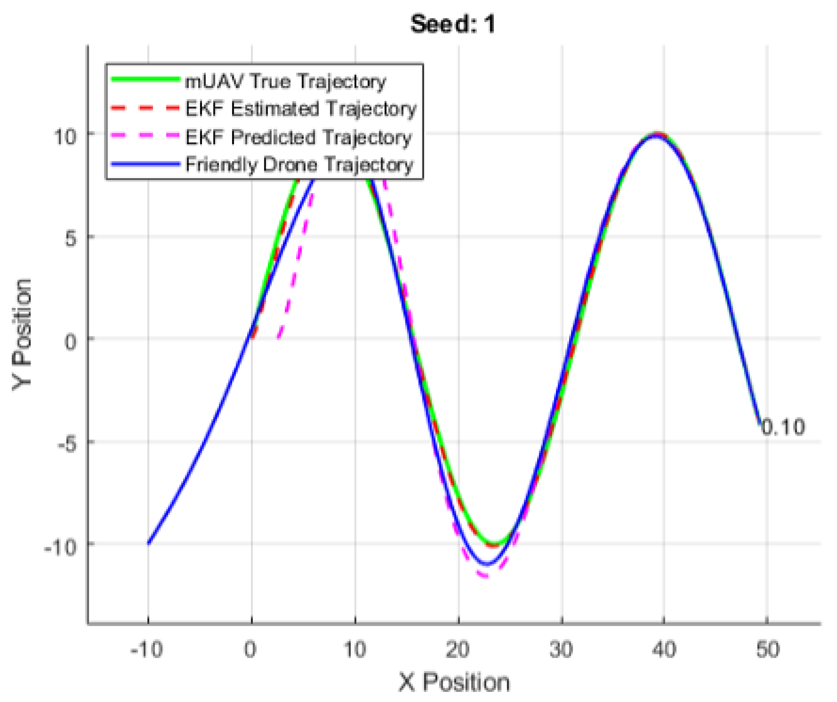
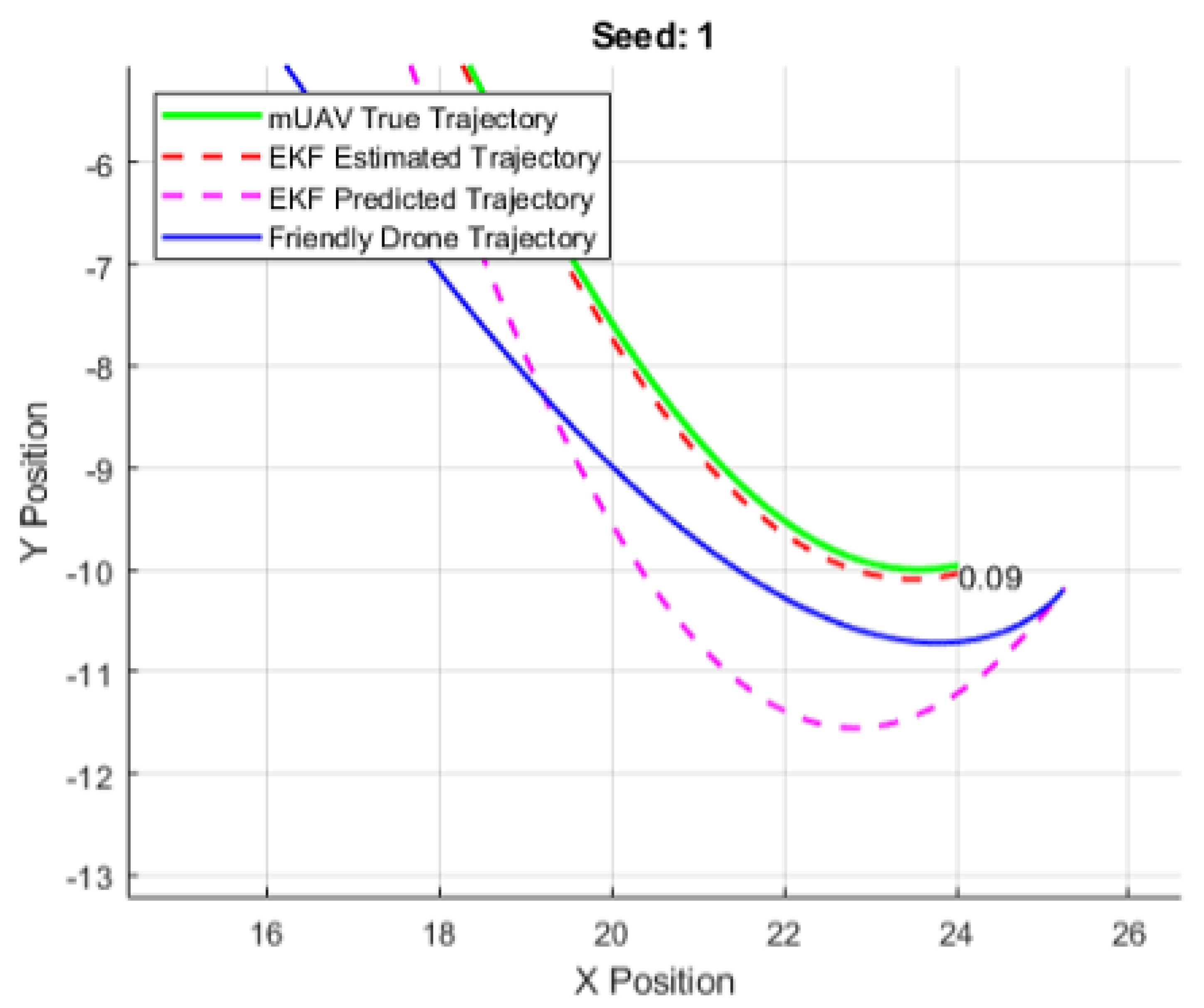
3.7. Performance on Linear Trajectory Models

The EKF state estimation method achieved a higher neutralisation rate (41%) compared to the PF method (30%) on linear leading mUAV models. Additionally, the TSET for EKF (0.018985 s) was significantly shorter than PF (9.508687 s). This indicates that the EKF method is more efficient when dealing with linear motion models.

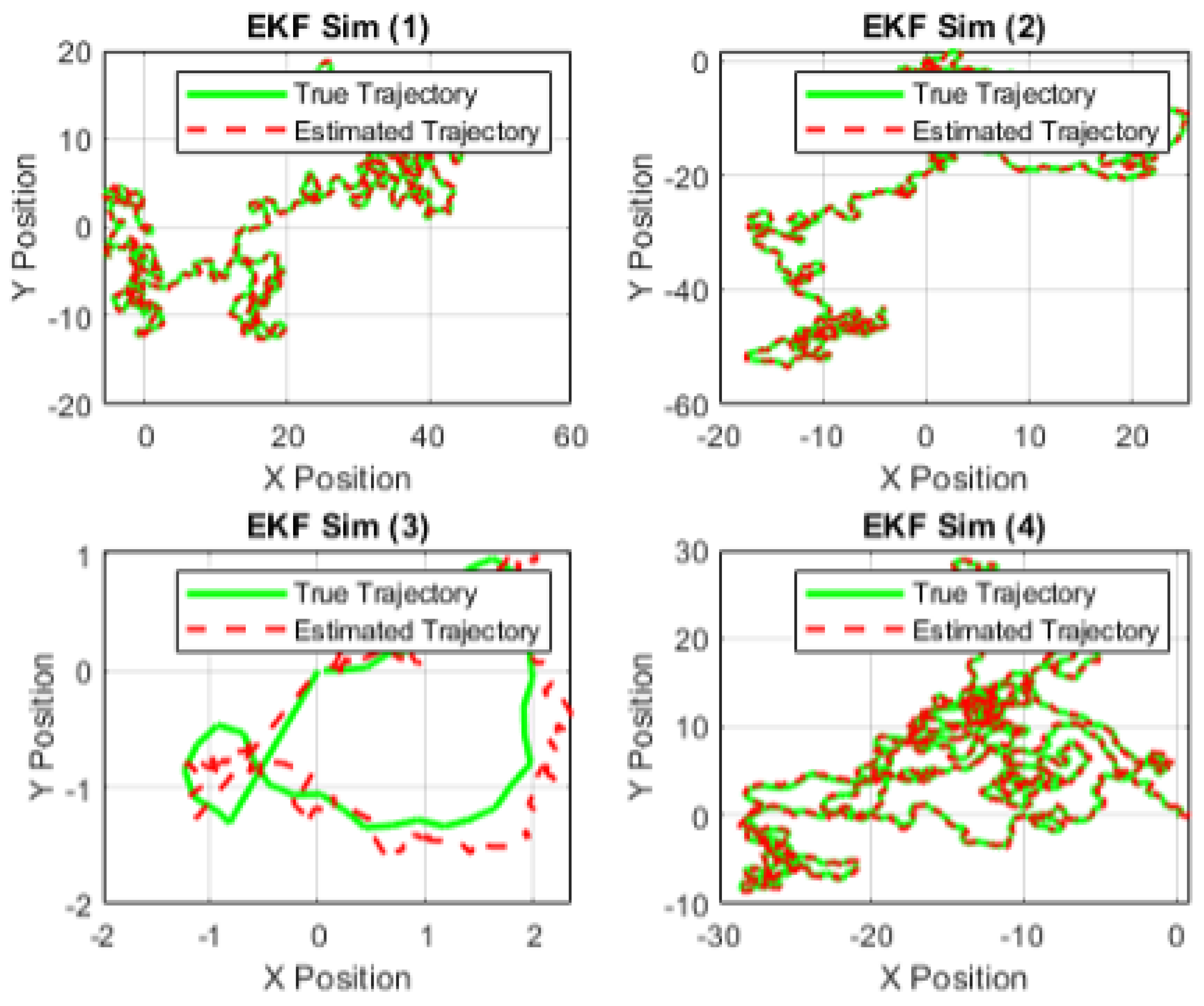
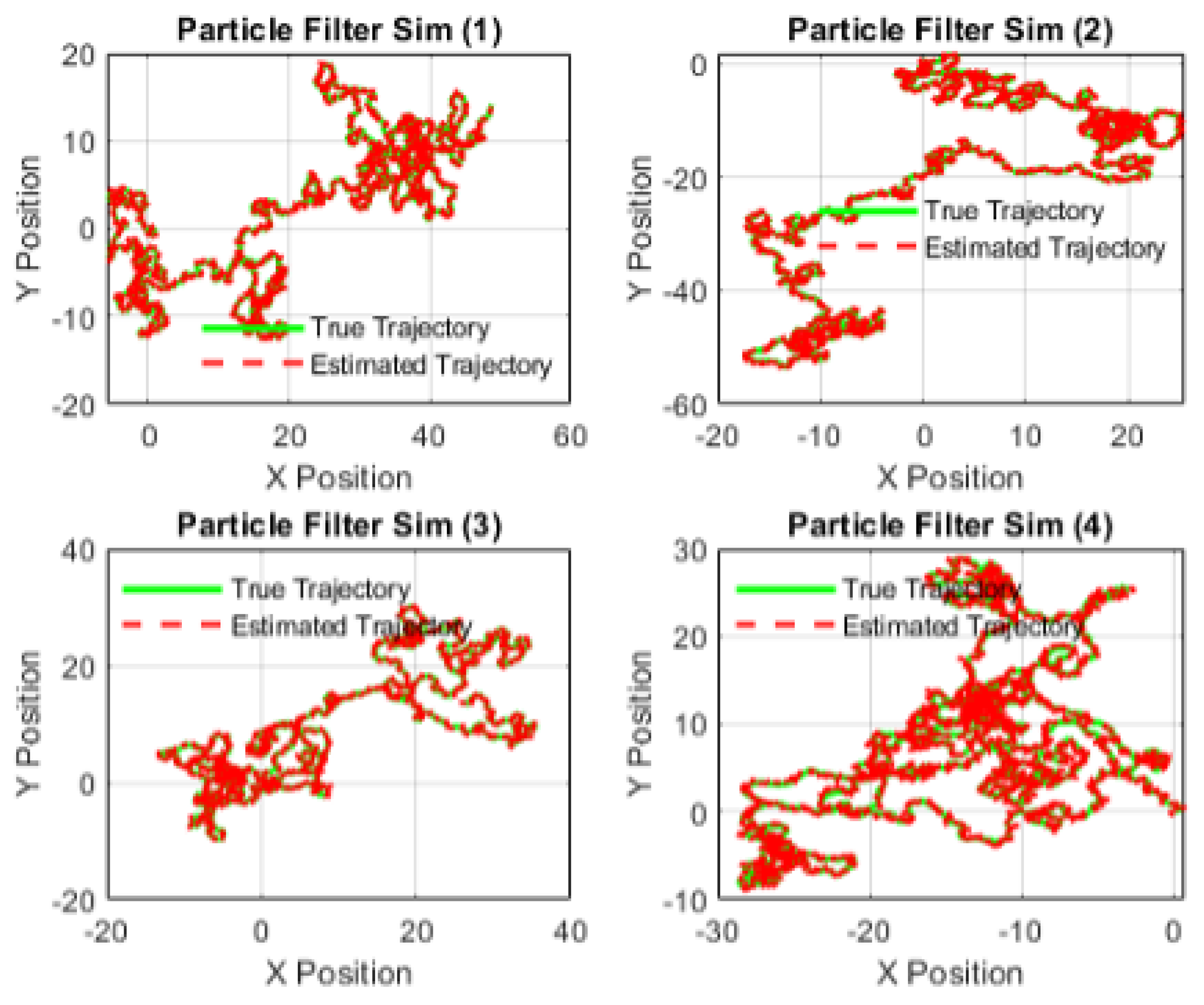
3.8. Performance on Stochastic Trajectory Models

Both the EKF and PF methods exhibited low neutralisation rates (5%). Furthermore, the PF method had a significantly higher TSET (0.744519 s) compared to the EKF method (0.029824 s). This low neutralisation rate could be attributed to the inherent difficulties in predicting stochastic trajectories.

3.9. Performance on Stochastic Trajectory Models with Enhancements

The EKF method, when enhanced with adaptive time horizon (ATH) and velocity control (VC), achieves substantial improvement, achieving a greater neutralisation rate (98%) with a relatively low TSET (0.011710s). This shows the critical role that ATH and VC have in the effective handling of the dynamic and evasive nature of stochastic trajectories. This suggests that the implementation of dynamic adjustment mechanisms significantly improves prediction accuracy and neutralisation capabilities, even under variable and uncertain conditions. Please see the following YouTube video for a side-by-side comparison: https://www.youtube.com/watch?v=m6rjXZ_pKpQ (accessed on 1 March 2025).

4. Discussion

The study currently examines the effectiveness of state estimation techniques, EKF and PF, for the neutralisation of leading mUAVs under varying trajectory conditions. In the pursuit of improving neutralisation success in both predictable and unpredictable motion models, the implementation of an adaptive time horizon (ATH) and dynamic velocity control (VC) was conducted.

4.1. Interpretation of Results

The results show that the EKF predictive method, when enhanced with ATH and VC, improves neutralisation rates compared to traditional PF methods and non-enhanced EKF methods. The success of the EKF method when dealing with a leading mUAV of a linear trajectory can be attributed to its robust state prediction capabilities, which efficiently handle Gaussian noise and relatively predictable motion patterns. However, the PF method, because of its higher computational intensity, renders it less suitable for real-time applications despite its theoretical advantages for nonlinear motion.

The significant improvement in the neutralisation rate in test 5 could also be attributed to the synergy between the ATH and VC measures and the performance of the EKF method in testing. The ATH and VC effectively adapted control logics to the context-specific dynamics of the leading mUAV, effectively negating the limitations of the EKF’s linear assumptions in nonlinear scenarios.

However, in stochastic trajectories, both filters exhibited limited efficacy, with neutralisation rates. This could be attributed to the inherent difficulty in accurately predicting evasive and nonlinear motion when using state estimation techniques. Nevertheless, the introduction of dynamic and adaptive mechanisms such as ATH and VC improves performance, suggesting that actively adapting predictions is crucial when handling stochastic movements.

4.2. Theoretical Implications and Practical Relevance

This study’s findings emphasise the importance of adaptive control strategies in counter-UAV systems. Incorporating ATH and VC into the EKF framework resulted in both lower TSET and higher neutralisation rates, which were beneficial. These results suggest that the incorporation of dynamic and adaptive mechanisms will significantly improve the probability of mission success.

From a pragmatic perspective, the successful implementation of ATH and VC can inform the development of more agile and responsive CUAS. The enhanced EKF model demonstrates an increased capability to predict the mUAV’s trajectory and provide effective navigation for the following drone to reduce response delays and increase neutralisation efficiency.

4.3. Limitations

Despite the promising results, multiple limitations exist within this study. There is a focus on only single-drone neutralisation scenarios which may not be applicable or generalisable to multi-agent scenarios. Additionally, this study was only conducted on drones in a two-dimensional space. Future work should investigate the application of coordinated neutralisation strategies with distributed guidance and control systems using multiple drones.

Furthermore, this study was conducted only on leading mUAVs with constant acceleration, which do not represent the full motion dynamics of actual UAVs. Auxiliary work on leading mUAVs with randomised or modelled acceleration and the inclusion of acceleration as a predicted/estimated state will further increase the real-life applicability of the methods discussed earlier.

Also, performance analyses were conducted only on the EKF method after initial testing due to the disparity in TSET. This means that tuned models of the PF were not thoroughly explored. More efficient implementations of PF could be explored in future work. By extension, the enhancements of ATH and VC were not tested with the PF model. These enhancements with PF methods remain a compelling future avenue that could be explored in future work.

Further research could also explore the integration of more other prediction algorithms such as model predictive control or receding horizon control. Additionally, other feedback control systems could be explored, such as linear quadratic regulators or PID-controllers. Furthermore, future work should explore the evaluation of the utilised system’s performance in more complex environmental conditions, which may include wind patterns and signal interference. This may enable us to gain deeper insights into the system’s real-world applicability.

5. Conclusions

This paper proposes a solution for the neutralisation of a leading mUAV using an autonomous following UAV. The position and state variables of the leading mUAV are provided to the following drone. The solution posed has provided good results in the test cases discussed in this paper.

This study establishes that the EKF, when enhanced with ATH and VC, thoroughly outperforms traditional PF methods as an effective solution for the real-time neutralisation of leading mUAVs. The method developed proved especially beneficial for linear and stochastic motion models, achieving high neutralisation rates with low TSET.

The findings highlight the importance of adaptive or dynamic control strategies in counter-UAV applications, which should serve as the foundation of resilient and efficient CUAS systems. Future research should focus on enhancing the prediction model’s adaptability and scope for various motion patterns.

References

1. Moreira, M.; Papp, E.; Ventura, R. Interception of non-cooperative UAVs. In Proceedings of the 2019 IEEE International Symposium on Safety, Security, and Rescue Robotics (SSRR), Würzburg, Germany, 2–4 September 2019. [Google Scholar]
2. Welch, G.; Bishop, G. An Introduction to the Kalman Filter; University of North Carolina at Chapel Hill: Chapel Hill, NC, USA, 1997. [Google Scholar]
3. Xu, X.; Li, C.; Zhuge, S.; Zhao, Z.; Yang, X.; Khoo, B.C.; Srigrarom, S.; Zhang, X. A buddy temporal-spatial calibration method for airborne sensors in multi-UAV systems. IEEE Robot. Autom. Lett. 2024, 9, 7365–7372. [Google Scholar] [CrossRef]
4. Abbas, M.T.; Jibran, M.A.; Afaq, M.; Song, W.-C. An adaptive approach to vehicle trajectory prediction using multimodel Kalman filter. Trans. Emerg. Telecommun. Tech. 2020, 31, e3734. [Google Scholar] [CrossRef]
5. Zhu, B.; Bin, Zaini, A.H.; Xie, L. Distributed guidance for interception by using multiple rotary-wing unmanned aerial vehicles. IEEE Trans. Ind. Electron. 2017, 64, 5648–5656. [Google Scholar] [CrossRef]
6. Wang, H.; Shi, Y. Design of uav target tracking controller based on visual servo. J. Phys. Conf. Ser. 2022, 2246, 012051. [Google Scholar] [CrossRef]
7. Chen, C.W.; Hung, H.A.; Yang, P.H.; Cheng, T.H. Visual servoing of a moving target by an unmanned aerial vehicle. Sensors 2021, 21, 5708. [Google Scholar] [CrossRef] [PubMed]
8. Jing, Z.; Pan, H.; Li, Y.; Dong, P. Non-Cooperative Target Tracking, Fusion and Control; Springer: Cham, Switzerland, 2018. [Google Scholar]
9. Chan, W.K.; Srigrarom, S. Image-based visual-servoing for air-to-air drone tracking & following with model predictive control. In Proceedings of the 2023 SICE International Symposium on Control Systems (SICE ISCS), Kusatsu, Japan, 9–11 March 2023. [Google Scholar]
10. Xia, B.; Mantegh, I.; Xie, W. UAV Multi-Dynamic Target Interception: A Hybrid Intelligent Method Using Deep Reinforcement Learning and Fuzzy Logic. Drones 2024, 8, 226. [Google Scholar] [CrossRef]
11. Song, X.; Yang, R.; Yin, C.; Tang, B. A cooperative aerial interception model based on multi-agent system for uavs. In Proceedings of the 2021 IEEE 5th Advanced Information Technology, Electronic and Automation Control Conference (IAEAC), Chongqing, China, 12–14 March 2021; pp. 873–882. [Google Scholar]
12. Prevost, J.; Desbiens, A.; Gagnon, E. Extended Kalman Filter for state estimation and trajectory prediction of a moving object detected by an unmanned aerial vehicle. In Proceedings of the 2007 American Control Conference, New York, NY, USA, 9–13 July 2007. [Google Scholar]
13. Lymperopoulos, I.; Lygeros, J. Adaptive aircraft trajectory prediction using particle filters. In Proceedings of the AIAA Guidance, Navigation and Control Conference and Exhibit, Honolulu, HI, USA, 18–21 August 2008. [Google Scholar] [CrossRef]
14. Ribeiro, M.I. Kalman and Extended Kalman Filters: Concept, Derivation, and Properties; Institute for Systems and Robotics, Instituto Superior Técnico: Lisbon, Portugal, 2004; Available online: https://www.researchgate.net/publication/2888846 (accessed on 1 March 2025).
15. Yang, Y.; Liu, X.; Zhang, W.; Liu, X.; Guo, Y. A Nonlinear Double Model for Multisensor-Integrated Navigation Using the Federated EKF Algorithm for Small UAVs. Sensors 2020, 20, 2974. [Google Scholar] [CrossRef] [PubMed]
Figure 1. EKF test on mUAV of linear trajectory (test 1).
Aerospace 12 00606 g001
Figure 2. PF Test on mUAV of linear trajectory (test 1).
Aerospace 12 00606 g002
Figure 3. Sample EKF tests on mUAV of stochastic trajectory (test 2).
Aerospace 12 00606 g003
Figure 4. Sample PF tests on mUAV of stochastic trajectory (test 2).
Aerospace 12 00606 g004
Figure 5. EKF test on mUAV of sinusoidal trajectory (test 3).
Aerospace 12 00606 g005
Figure 6. One case of overshooting (test 3).
Aerospace 12 00606 g006
Figure 7. EKF test on sinusoidal trajectory with ATH and VC) (test 5).
Aerospace 12 00606 g007
Figure 8. EKF test on mUAV with stochastic trajectory (with ATH and VC). The descriptions of the line style and colors are the same as in Figure 7.
Aerospace 12 00606 g008