Advancing Aviation Safety Through Predictive Maintenance: A Machine Learning Approach for Carbon Brake Wear Severity Classification

Abstract

Braking systems are essential to aircraft safety and operational efficiency; however, the variability of carbon brake wear, driven by the intricate interplay of operational and environmental factors, presents challenges for effective maintenance planning. This effort leverages machine learning classifiers to predict wear severity using operational data from an airline’s wide-body fleet equipped with wear pin sensors that measure the percentage of carbon pad remaining on each brake. Aircraft-specific metrics from flight data are augmented with weather and airport parameters from FlightAware^® to better capture the operational environment. Through a systematic benchmarking of multiple classifiers, combined with structured hyperparameter tuning and uncertainty quantification, LGBM and Decision Tree models emerge as top performers, achieving predictive accuracies of up to 98.92%. The inclusion of environmental variables substantially improves model performance, with relative humidity and wind direction identified as key predictors. While machine learning has been extensively applied to predictive maintenance contexts, this work advances the field of brake wear prediction by integrating a comprehensive dataset that incorporates operational, environmental, and airport-specific features. In doing so, it addresses a notable gap in the existing literature regarding the impact of contextual variables on brake wear prediction.

1. Introduction

Aircraft braking systems play an essential role in ensuring both operational safety and efficiency. Carbon brake pads, more specifically, are critical, as they undergo substantial stress during landing events and their performance directly affects an aircraft’s ability to decelerate and stop safely [1]. The degradation rate of carbon brake pads is highly variable and influenced by a complex interplay of operational and environmental factors. Specifically, operational variables such as landing frequency and runway length, along with environmental conditions like temperature and humidity, are known to impact the rate of brake wear [2]. This variability poses considerable challenges for maintenance planning and operational decision-making, underscoring the need for a more nuanced understanding of the factors contributing to brake wear.

Traditional maintenance strategies for aircraft braking systems have typically been either reactive or based on fixed intervals, and as such often failed to accurately reflect the actual condition of the brake pads. Such strategies can lead to either redundant maintenance actions or, conversely, missed safety-critical interventions if brakes degrade more rapidly than expected, compromising safety as a result [3]. The advent of advanced sensor technologies and Machine Learning/Artificial Intelligence (ML/AI) is enabling a paradigm shift toward predictive maintenance approaches [4]. For example, electronically actuated carbon brakes on certain wide-body aircraft are equipped with wear pin sensors that estimate the remaining thickness of the brake pad. These wear pin measurements, which serve as the primary signal for assessing brake wear, are typically recorded at irregular intervals, often only once every ten flights. The sensor value reflects the length of a physical pin embedded in each brake pad; as the pad material wears down, the pin retracts and eventually becomes flush with a reference surface, indicating that the pad requires replacement.

By analyzing these wear pin signals over time, it is possible to estimate brake degradation on a per-flight basis and classify it into categories such as High, Medium, or Low wear. This labeled dataset forms the basis for training supervised ML algorithms capable of predicting brake wear severity [5,6]. ML classifiers can leverage such labeled data to predict distinct levels of brake pad degradation. An effective classifier that integrates aircraft-specific parameters, environmental conditions, and airport characteristics can not only achieve high predictive accuracy but also help identify the main operational contributors to accelerated brake wear. These insights can then be used to proactively identify aircraft exhibiting persistent high-wear levels and prioritize them for maintenance interventions. More broadly, the ability to accurately predict brake wear severity enables airlines to optimize maintenance scheduling, minimize unplanned downtime, and improve resource allocation efficiency [7].

The remainder of the paper is organized as follows. Section 2 reviews the current state of the art in brake wear assessment within the automotive and aerospace industries and highlights the contributions of this study. Section 3 outlines the proposed methodology, while Section 4 describes its implementation, including the classification techniques employed and the evaluation metrics applied. Section 5 presents and discusses the results. Finally, Section 6 summarizes the findings, discusses their implications and limitations, and outlines directions for future research.

2. Literature Review

This section provides a synthesis of the existing literature and discusses the advancements and challenges associated with forecasting brake wear in the automotive and aerospace industries.

2.1. A Lack of Consideration for the Operational and Environmental Contexts

Brake wear predictions have traditionally relied on limited data that often overlook important environmental and operational factors. For instance, Oikonomou et al. estimated the Remaining Useful Life (RUL) of brakes using only the count of past flights and a single sensor reading as indicators of the remaining brake pad thickness [8]. This approach neglected environmental variables such as ambient air temperature and specific aircraft metrics such as weight and speed. They also averaged the data across six flights, diminishing the model’s sensitivity to immediate wear events possibly triggered by various operational or environmental conditions [8]. Similarly, Hsu et al. noted significant fluctuations in their health indicators and variability in brake wear potentially attributed to external factors, usage intensity, and aircraft age. However, their analysis did not account for such factors. Instead, they, too, employed a moving average to reduce noise effects, creating a new health indicator that weakened the model’s sensitivity to rapid degradation events [9].

Regarding the impact of weather conditions more specifically, Travnik et al. highlighted the significant role of relative humidity and air temperature in friction-limited landings [10]. Yet, a comprehensive understanding of operating and environmental contributors to carbon brake wear remains elusive. Finally, given the limited availability of accessible, real-time operational data, Steffan et al. noted the need for simulations or experimental data to predict brake wear rates [11].

2.2. A Lack of Representation of the Operational Variability in Vehicle Dynamics

A substantial body of research relies on simulated data generated through software tools or test apparatus. However, these environments often hold important variables, such as speed and pressure, constant, thereby failing to capture and mirror the inherent complexity and variability of real-world operations. For example, Magargle et al. developed a physics-based model for automotive braking systems, yet their approach did not incorporate real-time vehicle data [12]. While effective in controlled scenarios, such models fall short in capturing the stochastic nature of actual vehicle behavior. Similarly, experimental setups frequently depend on simplifying assumptions about degradation processes. For example, Küfner et al. employed a linear wear hypothesis, which may not align with the nonlinear wear patterns observed in service conditions [13]. De Martin et al.’s simulations also assumed idealized symmetric landings, a scenario often challenged in reality by strong crosswinds [14]. Finally, Cao et al. highlighted the discrepancies between test conditions and actual operational environments, calling for testing protocols that better replicate actual operational conditions [15]. However, achieving such fidelity would require exhaustive and resource-intensive experimentation, which may still not fully capture the operational variability in vehicle dynamics.

2.3. A Shift from Traditional Models to ML Approaches

Many studies have traditionally relied on physical or statistical approaches for degradation modeling. However, as Cao et al. discussed, these techniques overlook abrupt changes and complex wear patterns [15]. Echoing this, Chetan et al. employed multivariate linear regression but acknowledged the potential benefits of using more complex ML techniques should data reflective of actual operational variability become available [16]. In contrast, Oikonomou et al. have demonstrated the superiority of ML models, such as Artificial Neural Networks (ANNs) with bootstrapping and Bayesian Linear Regression (BLR), over traditional statistical models like Non-Homogeneous Hidden Semi-Markov Models (NHHSMM), even in cases where the inputs and brake RUL exhibit a direct linear correlation. They advocated for applying more sophisticated algorithms to capture the nuanced dynamics of brake wear [8]. Yet, such models’ predictive strengths and accuracies are often constrained by the limited datasets on which they are trained. Burnaev, for instance, suggested that the complex model they developed, which combines deep Recurrent Neural Networks (RNNs) with an eXtreme Gradient Boosting (XGBoost) framework, would likely perform better with a more extensive training dataset [17]. As such, the imperative exists for more expansive data collection and fusion.

2.4. Need for ML Model Interpretability and Uncertainty Quantification

Another key limitation of current modeling approaches lies in the interpretability and operational feasibility of the results they generate. Burnaev has highlighted that contemporary deep learning techniques, such as RNNs, are inherently opaque and present significant challenges for real-time deployment in onboard systems due to their high computational demand [17]. Moreover, a persistent issue in the field is the application of these complex models without adequate consideration of predictive uncertainty. For example, Choudhuri et al. applied ANNs for modeling brake wear without incorporating any uncertainty quantification [18]. In contrast, Oikonomou et al. emphasized the necessity of accounting for prediction uncertainty, particularly given the stochastic nature of operational data, and integrated appropriate methods to address this challenge in their work [8].

2.5. Balancing Trial-And-Error with Computational Constraints for Hyperparameter Tuning

A commonly cited limitation in the literature is the absence of a systematic approach to the offline optimization of algorithms, particularly in selecting appropriate models and fine-tuning their hyperparameters. In many cases, optimal configurations are identified through ad hoc trial-and-error methods rather than through rigorous, structured optimization. For instance, in Küfner et al.’s study involving RNNs, the number of hidden layers was constrained by the computational limitations of the edge devices used, rather than by performance-based criteria [13]. Similarly, Burnaev’s work lacks a detailed explanation for the choice of hyperparameters across various models, leaving their selection process ambiguous [17].

2.6. Observations from the Literature and Statement of Research Contributions

The literature review identifies important and persistent gaps that undermine the efficacy of existing approaches to aircraft brake wear prediction:

• Insufficient integration of operational and environmental context: Most prior studies rely on sparse datasets, often overlooking important variables such as aircraft-specific metrics, operational factors, weather conditions, and airport characteristics. This highlights the need for a comprehensive and representative dataset that captures the interactions among these factors.
• Limited representation of real-world operational variability: Many studies rely on simulations or controlled experiments that hold certain variables (e.g., speed, pressure) constant, failing to capture the dynamic and unpredictable nature of real-world vehicle operations. This limits model generalizability and applicability and underscores the need for data that reflects true operational variability in aircraft dynamics.
• Incomplete adoption of robust ML techniques due to limited data: While ML models show promise in capturing complex wear patterns, their performance is often constrained by limited, non-representative training data. This highlights the need for broader data collection and integration.
• Lack of interpretability and uncertainty quantification in ML models: Deep learning models used in prior studies are often opaque and computationally intensive, hindering their deployment in real-time systems. Moreover, few studies quantify predictive uncertainty, which is essential for safety-critical applications like brake wear prediction.
• Lack of systematic hyperparameter optimization: Many studies rely on trial-and-error methods for model selection and tuning, often constrained by computational resources and lacking transparency in the optimization process.

To address these gaps and advance the predictive maintenance of aircraft braking systems, this study proposes the following innovative elements as contributions to the existing state of the art:

• Comprehensive data utilization: Real-world flight operations data from a commercial airline is integrated with environmental and airport context from FlightAware^®, resulting in a rich and multidimensional dataset suitable for ML model training.
• Rigorous benchmarking of classification approaches: A supervised learning pipeline is developed to systematically evaluate and compare a wide range of classifiers, including interpretable models such as Logistic Regression and Decision Trees, and high-performance ensemble methods such as XGBoost and Categorical Boosting (CatBoost).
• Structured hyperparameter optimization: Grid search with cross-validation is employed to systematically tune model parameters and enhance predictive accuracy across all algorithms.
• Influential factor analysis: The most significant features driving brake wear severity are identified to guide actionable insights for airline operations and maintenance planning.
• Uncertainty measurement: Uncertainty quantification is incorporated to reflect the stochastic nature of operational data, thereby improving the reliability of maintenance recommendations.

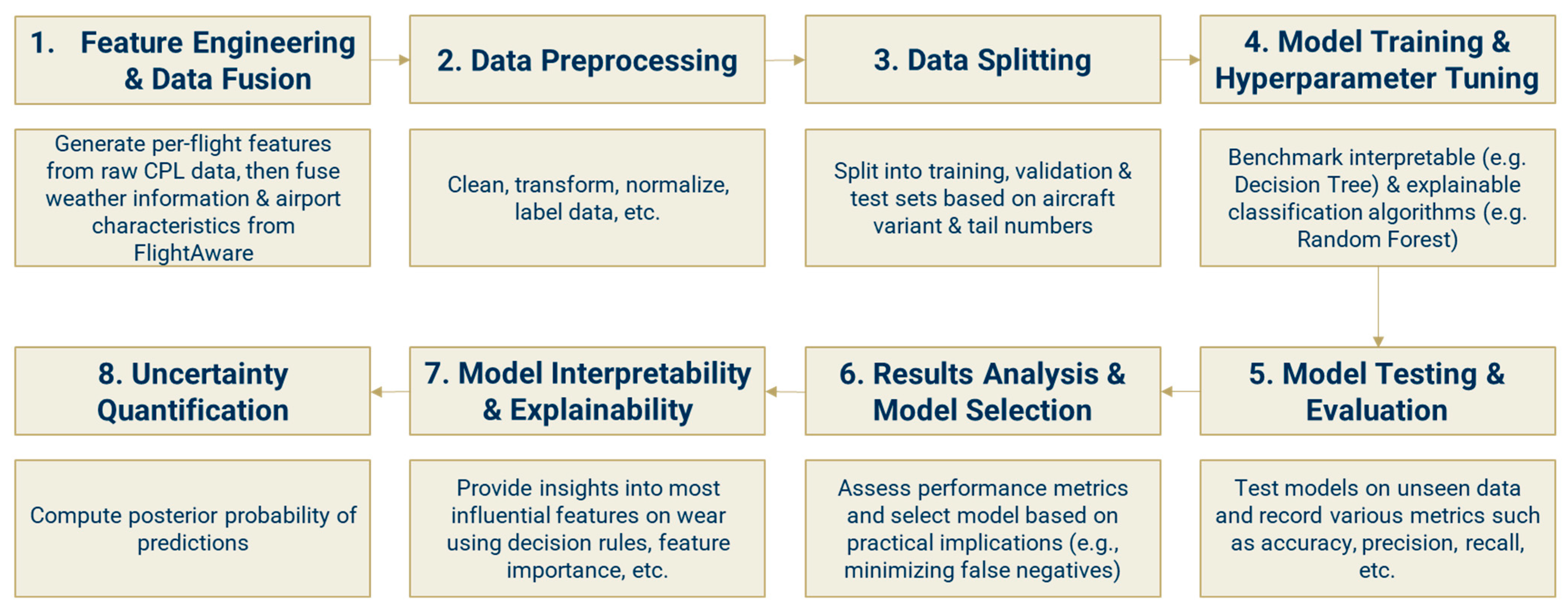
3. Methodology

A dataset from a fleet of a specific wide-body aircraft, which includes, among its many features, electronic wear pin values, is used for the training of supervised ML techniques to predict the severity of carbon brake pad degradation. Supervised ML leverages datasets with predefined labels to train models capable of making accurate predictions [5,6]. The proposed methodology involves categorizing flight data, including a mix of aircraft-specific metrics and operational and environmental conditions, into various degrees of brake wear (high, medium, or low) using quantile-based labeling. The wear pin signal, which indicates the remaining thickness of the carbon brake pad as a percentage rounded to the nearest whole number, exhibits a decreasing step-function pattern and typically shows an inconsistent reduction approximately every ten flights. Interpolation methods convert this signal into a smooth, continuous curve. Labels are then generated to represent the severity of carbon brake pad wear per flight, determined by binning the change in interpolated wear pin values from one flight to the next into quantiles. This classification aids in swiftly pinpointing unusually high brake wear on specific aircraft, thus facilitating early maintenance intervention when necessary.

A range of ML classifiers is considered for this problem, which includes linear classifiers, Support Vector Machines (SVMs), Decision Trees (DT), and Random Forests [19,20,21,22,23]. Linear classifiers divide data points into categories based on a linear boundary, whereas SVMs aim to find the most effective hyperplane separation between different classes for more precise classification [19,23]. Conversely, Decision Trees and Random Forests are tree-based methods that categorize data by sequentially splitting it according to the values of certain features [20,21,22]. Through a benchmark of these techniques and others, classification yields a distinct prediction of brake wear levels, enhancing the detection of unusual wear trends.

The steps that form the proposed methodology are represented in Figure 1. We first engineer features from the raw flight data and fuse them with weather and airport information from FlightAware^® to create a comprehensive dataset [24]. Next, the data is preprocessed, which involves cleaning, transforming, and normalizing the data. A label column is then generated, which serves as the target variable in subsequent classification models. Then, the dataset is segregated into training, validation, and testing sets based on aircraft tail numbers. After splitting the data, a suite of classification algorithms is trained and refined using hyperparameter optimization. Once each algorithm has been tuned, the resulting models are applied to the test set to evaluate their performance on previously unseen data, using standard classification metrics to assess model performance. Next, the results are analyzed and the model that best balances accuracy with practicality (e.g., minimizing false negatives) is selected. Deeper insights into the classification outcomes are also provided using feature importance and/or decision rules. Finally, the uncertainty in the predictions is quantified by computing the posterior probability of predictions. In doing so, a probabilistic understanding of the model outputs is provided. This structured approach ensures a rigorous evaluation of carbon brake wear severity with a strong emphasis on both model accuracy and comprehensibility.

The subsequent section provides additional details for each of the steps in Figure 1.

4. Implementation

This section provides an in-depth discussion of the implementation of each step of the methodology.

4.1. Step 1: Feature Engineering and Data Fusion

The primary data source is Continuous Parameter Logging (CPL) data, which encapsulates various parameters from diverse systems aboard an aircraft throughout its flight, including engine performance data, avionics data, and other system diagnostics information continuously recorded for maintenance, analysis, and operational optimization purposes. This comprehensive dataset, recorded on a 1 Hz frequency (i.e., one recording per second), offers a detailed account of aircraft operation from engine start to shut down. The resultant CSV files generated post-flight are rich information repositories, encompassing over 800 parameters and varying in size based on the duration of the flight. This expansive data originates from an airline’s fleet of 71 wide-body aircraft, segmented into 36 units of a smaller variant, 32 units of a medium variant, and 3 units of a larger variant, each tailored to meet specific market demands with variations in seat capacity and range [25].

The focus is on the aircraft’s braking system, particularly the eight carbon brakes on each plane, which are electronically actuated and integrated with sensors [1]. These sensors play a key role in measuring the remaining brake pad thickness, albeit with a notable limitation in data granularity, as each percentage of brake pad remaining is reported to the nearest integer value. Furthermore, the infrequent reporting of the wear pin value (approximately every ten flights) introduces an additional layer of approximation, with the wear pin signal being rendered as a step function characterized by periods of constant values followed by sudden decreases, as shown in Figure 2.

The airline’s CPL data, accessible since July 2017, includes hundreds of thousands of full-flight files. However, given the large number of parameters recorded, a necessary step in the process involves leveraging subject matter expertise to guide the down-selection of parameters directly relevant to brake wear, e.g., brake parameters (e.g., brake temperature), environmental factors (e.g., static air temperature), and pilot inputs (e.g., autobrake and thrust reverser usage). This helps ensure that only the most impactful features are retained for modeling. Note that the complete list of extracted CPL parameters is not disclosed due to intellectual property considerations.

To avoid the computational burden associated with high-resolution, per-second data, which could overwhelm certain ML models, a feature engineering approach is adopted that generates per-flight summary features for each aircraft’s eight brakes [26]. These features are derived across different phases of flight to ensure a comprehensive representation and understanding of brake system performance during taxi out (covering Power On, Engine Start, Taxi Out, and Takeoff Roll), landing (encompassing Flare and Rollout), and taxi in (including Taxi In, Engine Shutdown, and Maintenance). For each phase, specific features, such as the mean cabin altitude, are generated to provide insights into the operational conditions that the brakes experience. Sample features generated for the brakes on each flight are listed in

Table 1. Sample Per-Flight Features Generated from CPL Data *.

Operational and Utilization Metrics	Aircraft, Technical, and Environmental Metrics	Wheels and Brakes Metrics		Pilot Inputs and Engine Metrics
Airport ICAO Codes	Aircraft ID/Tail Number	Brake Position	Mean Wheel Speed *	Autobrake Setting
Flight Start/End Timestamps	Aircraft Class	Wear Pin Value	Wheel Energy *	Thrust Reverser Usage
Tail Flight Number	Mean Ground Speed *	Brake Command (CMD) Fraction *	Mean Brake CMD *	Mean Captain or First Officer Pedal Force *
Flight Duration	Deceleration *	Number of Brake Applications *	Mean and Max Brake Temperature Monitoring System (BTMS) Brake Temperature *	Mean Engine N1 Left/Right *
Tail Flight Count Per Day	Aircraft Weight *	Mean Autobrake Master CMD *
Rolling Average Flights/Day (Window: 100 Flights)	Mean Kinetic Energy *	Mean Tire Pressure *
Time Between Flights	Mean Cabin Altitude *	Wheel Wear *
Time Duration *	Static Air Temperature *	Mean Electronic Brake Actuator Force *
Tail Flight Number of the Day		Parking Brake Sum *

* Features marked with an asterisk (*) are calculated for each of the three flight phases: taxi out, landing, and taxi in.

.

The secondary data source leveraged for this effort is FlightAware^®, (Houston, TX, USA) which offers real-time flight tracking and data analysis services [24]. It serves as a repository for weather information at the arrival airports. Its weather data is primarily derived from Meteorological Aerodrome Reports (METARs), standardized to provide weather observations at airports worldwide. These reports include information such as temperature, cloud cover, and atmospheric pressure, among other meteorological variables [27]. Weather parameters from FlightAware^®, including Cloud Altitude, Pressure, Air Temperature, Dew Point, Relative Humidity, Visibility, and Wind Speed/Direction/Gust, have been available since April 2021; consequently, the data utilized in this research spans from April 2021 until October 2023.

Incorporating weather data is essential for understanding the environmental conditions aircraft are exposed to, especially during the critical phases of landing and taxiing. Weather conditions can alter planned aircraft operations and profoundly impact braking system performance [28]. For example, wet or icy runways can significantly affect braking efficiency, and atmospheric conditions can influence aircraft performance and brake wear [29]. CPL data is fused with weather information from FlightAware^® based on the arrival airport and the time of arrival (UTC). This temporal alignment helps guarantee the relevance of the weather data associated with the specific flight conditions experienced by the aircraft. By merging weather data with the intricate operational details obtained from CPL data, the dataset provides a more holistic understanding of the various elements influencing brake wear.

FlightAware^® also offers airport-specific data, which encompasses aggregated runway information, including parameters such as average, minimum, and maximum runway lengths, and geographical details such as latitude, longitude, and elevation [30]. However, it is essential to note that this information is presented in a generalized format, with only one row of data provided for each airport. As such, the data does not distinguish between different runways within the same airport, which could limit the precision of analyses requiring runway-specific details. Despite this limitation, the aggregated airport data is still a valuable resource as it provides information about an airport’s overall size and layout, which can have significant implications for aircraft operations. For instance, the length of runways can influence the required braking force and, consequently, the wear on brake pads. Similarly, the airport’s elevation and location may impact environmental conditions affecting aircraft performance.

In summary, integrating CPL data with environmental and airport-specific variables yields a dataset well-suited for the application of machine learning techniques to predict carbon brake wear. Beyond supporting predictive modeling, this enriched dataset also offers the potential to uncover deeper insights into the complex interactions among the factors contributing to brake wear.

4.2. Step 1: Data Preprocessing

The subsequent section delves into the steps taken to preprocess the data and ensure that the dataset is primed for model training.

4.2.1. Feature Exclusion Based on Correlation

The meticulous approach to refining the dataset and enhancing the reliability of the predictive models begins by eliminating highly correlated features, utilizing a Pearson correlation coefficient threshold of 0.95 as the criterion for exclusion. This step is predicated on the understanding that retaining variables that exhibit high correlation can introduce redundancy into the model, potentially skewing the results or leading to multicollinearity issues [31,32].

A notable example of this pruning involves the mean actuator forces, where four actuators control each brake [1]. These forces are highly correlated with the brake command, representing a composite measure incorporating both the brake application force and the anti-skid command. Given the redundancy, these actuator force variables are deemed excessive and dropped from the dataset. Similarly, the mean N1 rotor speeds of the left and right engine low spool fans exhibit a high degree of correlation. As a result, it was decided to retain only the data from the left engine’s fan, thereby eliminating unnecessary duplication without compromising the integrity of the dataset. Another significant correlation is observed between the pedal forces applied by the first officer and the captain, a built-in redundancy for enhanced safety and control, which requires excluding one of these variables to streamline the dataset [1]. Through these eliminations, the preprocessing stage allows for keeping only those variables that are independent from one another.

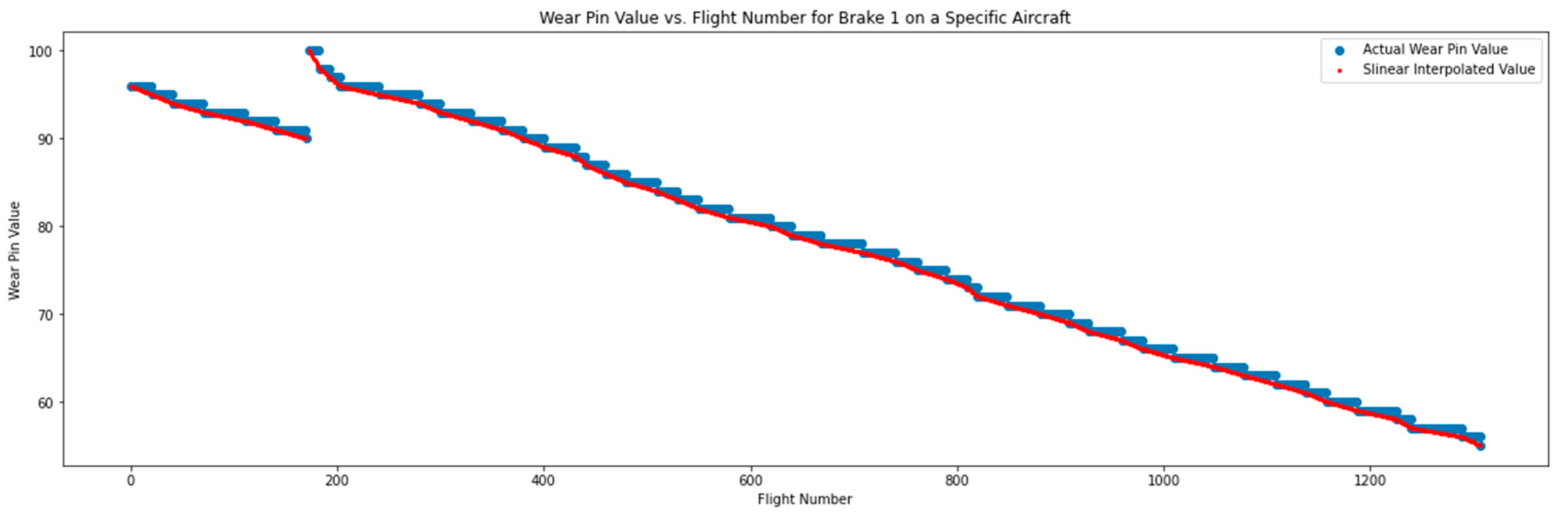
4.2.2. Wear Pin Value Correction and Interpolation

The next stage of the data preprocessing phase aims to refine the reported wear pin signals from CPL data. The wear pin values are reported inconsistently (approximately every ten flights), resulting in a step-function data pattern, as shown in Figure 2 for a specific aircraft brake, which requires smoothing and interpolation.

Before interpolation, the dataset is segmented based on unique aircraft identifiers (i.e., tail numbers) and brake positions, with further subdivision around instances of significant wear pin value changes suggestive of brake maintenance or replacement, as depicted by the green arrow in Figure 2. Zero values are filled within these segments, employing a forward-fill strategy to handle missing data points sensibly [33,34]. Next, the wear pin value is corrected for data errors such as sudden slight increases or null values. The wear pin signal should decrease monotonically, reflecting the physical reality that brake pads can only wear down over time unless replaced.

Subsequently, various interpolation methods are applied, including linear, quadratic, cubic, and Piecewise Cubic Hermite Interpolating Polynomials (i.e., PCHIP) [35,36,37,38,39]. Note that the various interpolation methods are leveraged from SciPy’s interpolate module. Each technique fits the corrected wear pin values to a smooth, continuous curve throughout flights. Figure 2 below shows the variation of the original and interpolated wear pin values, using a linear spline (i.e., slinear), as a function of the flight number. Edge cases, where the number of data points between replacements may be insufficient for certain types of interpolation, are also handled.

When comparing interpolation methods, the linear spline demonstrated the best fit to the original wear pin values, as evidenced by its performance across several statistical measures: Mean Absolute Error (MAE), Mean Squared Error (MSE), Root Mean Squared Error (RMSE), and RMSE to range ratio, as reported in

Table 2. Evaluation Metrics for Various Interpolation Methods.

Interpolation Method	MAE	MSE	RMSE	RMSE/Range	% Positive Degradation Introduced
linear	0.4895	0.3324	0.5765	0.0058	0
slinear	0.4895	0.3324	0.5765	0.0058	0
quadratic	0.5021	0.3696	0.608	0.0061	1.7298
cubic	0.5039	0.3772	0.6141	0.0062	1.5278
pchip	0.4914	0.3338	0.5778	0.0058	0
akima	0.4913	0.3331	0.5771	0.0058	0.2711

below [40]. These metrics help assess the accuracy and reliability of interpolation methods by quantifying the deviation between the interpolated values and the original data points.

The linear spline method for interpolating wear pin values aligns well with the nature of the data as it refers to a straightforward linear interpolation between two points. It is adequate for data that changes relatively constantly over time or where a direct relationship can be assumed between consecutive data points [39,41]. This method is more intuitive and computationally less intensive than higher-order polynomial or spline interpolations, which can overfit the data and sometimes introduce non-physical positive brake degradation rates, as reported in Table 2 [39,41]. In addition, the linear spline balances accuracy and computational efficiency, making it suitable for near-real-time applications where rapid data processing is essential [39,41]. As a result, this interpolation method is selected as the preferred interpolation technique for the results detailed throughout the remainder of this paper.

After interpolation, the per-flight degradation is computed by evaluating the differences in interpolated wear pin values between consecutive flights. In parallel, cumulative degradation is tracked relative to the initial brake pad thickness at the time of installation. Constraints are also enforced to ensure that interpolated values remain within realistic bounds, defined by the original maximum and minimum wear pin values. This step is important for maintaining the integrity of the data and preventing extrapolated values from exceeding plausible limits. Finally, the processed segments are concatenated into a comprehensive data frame, consolidating the enhanced, interpolated brake wear data across all aircraft and brakes.

4.2.3. Averaging Feature Values over Constant Wear Pin Segments

The wear pin signal is used to label the data in the subsequent step of the preprocessing stage. However, the poor resolution of this signal, which is constant over approximately every ten flights and is reported to the nearest integer value, introduces a notable challenge for ML modeling, especially considering the variety of operational conditions and environmental factors an aircraft may encounter across these intervals. For instance, flights might vary significantly in duration, weight load, runway conditions, and weather, affecting brake wear differently. However, due to the wear pin value being updated infrequently and rounded to the nearest whole number, substantial changes in brake pad condition are not reflected in the data for several flights. In other words, even after interpolating the wear pin values, the per-flight degradation remains similar for the flights during which the original wear pin value stays the same despite experiencing drastically different operating and environmental conditions. This inconsistency makes it difficult for ML models to distinguish between distinct levels of brake wear. The models must navigate these intervals of static wear pin values despite underlying changes in wear patterns, complicating their ability to generate precise and reliable predictions about the target condition of the brake pads.

To address this issue, feature values are averaged over segments in which the wear pin measurement remains constant. For each aircraft and brake combination, the data is divided into smaller segments bounded by brake replacements to isolate individual wear cycles. Within each segment of constant wear pin value, feature values are averaged, and the segment length, representing the number of flights during which the wear pin value does not change, is computed and added as a new feature. This process efficiently condenses the dataset into a format that emphasizes the average conditions experienced by each brake as the wear pin remains unchanged, thus facilitating a clearer understanding of the relationship between operational parameters and brake wear.

4.2.4. Data Labeling and Outlier Identification

Labels are critical to the use of supervised ML approaches for classification [5,6]. This research defines labels that categorize the average per-flight degradation into discrete classes based on quantile thresholds. Note that the average per-flight degradation rates for the brake wear pin values are smoothed according to their respective interpolation method. Based on quantiles, these values are then categorized into three levels (i.e., High, Medium, and Low wear), ensuring that each category has an approximately equal number of data points. Since different interpolation methods lead to distinct distributions of the interpolated wear pin signal, the quantile thresholds for each method vary, as shown in

Table 3. Quantile Thresholds to Label Data Based on Various Interpolation Methods.

Interpolation Method	Lower Bound—High Wear	Upper Bound—High Wear	Lower Bound—Low Wear	Upper Bound—Low Wear
linear	−1.0000	−0.0492	−0.0335	−0.0051
slinear	−1.0000	−0.0492	−0.0335	−0.0051
quadratic	−1.7749	−0.0499	−0.0334	0.0612
cubic	−1.7621	−0.0499	−0.0334	0.0707
pchip	−1.0000	−0.0499	−0.0334	−0.0001
akima	−1.0000	−0.0500	−0.0334	0.0000

. For example, with slinear interpolation, flights are categorized as High wear if the average per-flight degradation is between −1 and −0.0492, Low wear if it is between −0.0335 and −0.0051, and Medium wear for values between −0.0492 and −0.0335.

Outliers (i.e., anomalies) can also be identified based on the average per-flight degradation rates derived from the interpolated wear pin signals. Assuming the average per-flight degradation is normally distributed, one method to identify outliers uses standard deviations. A common choice is to use three standard deviations based on the empirical rule that approximately 99.7% of data in a normal distribution are within this range from the mean. Thus, lower and upper thresholds for brake wear are established to delineate the boundaries beyond which data points are considered outliers [42,43]. As such, the data can be categorized as ‘normal’, ‘high’, or ‘low’ based on the average per-flight degradation value relative to the outlier thresholds. This process helps recognize and potentially exclude anomalous data points that could skew the predictive models.

4.2.5. Handling Missing Data and Scaling Numerical Features

The concluding stages of data preprocessing involve handling missing values to preserve the dataset’s integrity and ensure its accuracy and consistency for further analysis. In this phase, rows exhibiting missing values are removed, eliminating potential biases or inaccuracies stemming from incomplete information [44]. A notable finding is that columns with missing data, detailed in

Table 4. Columns with Missing Values.

Column *	Missing %
Average Wheel Speed (Taxi Out) *	8.207
Average Wheel Speed (Landing) *	8.207
Average Wheel Speed (Taxi In) *	8.207
Average Cloud Altitude Upon Arrival **	1.931
Average Air Temperature Upon Arrival **	1.078
Average Pressure Upon Arrival **	1.078
Average Dew Point Upon Arrival **	1.078
Average Relative Humidity Upon Arrival **	1.078
Average Wind Gust Upon Arrival **	1.078
Average Wind Speed Upon Arrival **	1.078
Average Wind Direction Upon Arrival **	1.078

* Columns marked with an (*) are sourced from CPL Data, while those marked with (**) are sourced from FlightAware^®.

, primarily pertain to mean wheel speed measurements for the flight phases of interest. These columns refer to the features averaged over flights experiencing constant wear pin value segments. After further investigation, the wheel speeds for wheels 7 and 8 are missing for approximately 30% of flights. Missing values are also observed in the FlightAware^® weather data, denoted by (**) in Table 4.

In ML, the performance of specific models is profoundly influenced by the scale of input features (i.e., range and distribution of values) [45]. To harmonize the feature scales, numerical columns within the dataset are subjected to scaling via the MinMaxScaler function from the scikit-learn library, which adjusts each feature to a [0, 1] range, ensuring that all features contribute equally to the model’s predictions [46,47]. After excluding rows with missing values (about 8% of the preprocessed data) and scaling features, the resulting dataset contains 31,157 entries across 93 columns and is ready for subsequent modeling. The next step involves splitting the data for training and testing purposes.

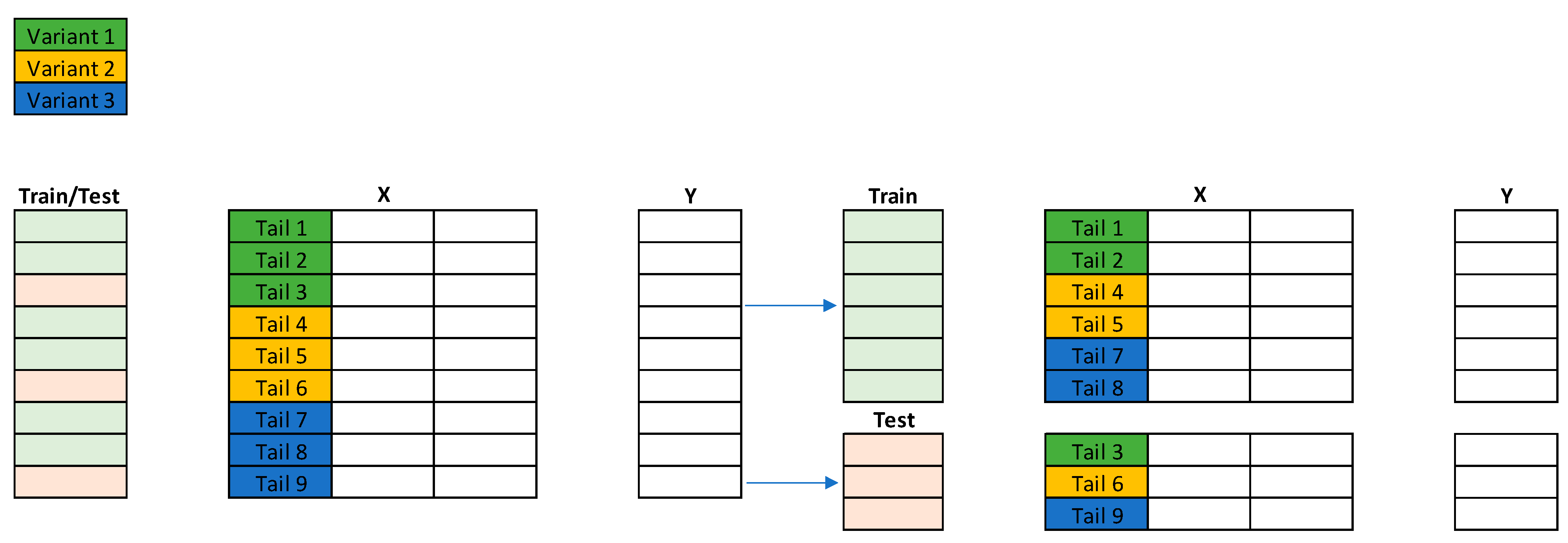
4.3. Step 3: Data Splitting

The data is split by aircraft variants and tail numbers into training and testing sets with a 70–30% ratio, ensuring balanced datasets where each tail’s unique operational and maintenance characteristics are preserved in one set to prevent bias. The dataset includes three variants of a wide-body aircraft (small, medium, and large). Each variant may experience different operational conditions (e.g., different routes, weights, or usage patterns) and may have distinct maintenance routines. By preserving these unique characteristics during data splitting, the model is trained and tested on data that accurately reflects the operational and maintenance profiles of each variant. This means that the specific features and behaviors of each aircraft type are maintained in both the training and testing sets, allowing the model to generalize well to real-world conditions.

The data splitting process is depicted in Figure 3, with the tail numbers for each variant split into 70% for training and 30% for testing. The training tail numbers from all variants are then combined to form the training dataset, and the testing tail numbers from all variants are combined to form the testing dataset. This deliberate segregation ensures that data points for a particular aircraft are exclusively allocated to one set, preventing data leakage and overlap. This approach enhances model generalizability and is particularly beneficial for evaluating the model’s predictive ability on aircraft not encountered during training, closely mimicking real-world scenarios where predictive maintenance models are applied to new and unseen aircraft.

4.4. Step 4: Model Training and Hyperparameter Tuning

As mentioned, the dataset features a label column that categorizes the wear of carbon brakes into three distinct severity levels—Low, Medium, and High—which allows for different approaches to training ML classifiers depending on how the classification problem is defined:

• Approach 1: Treating the problem as a multiclass classification task, aiming to accurately predict each of the three labels: ‘Low’, ‘Medium’, and ‘High’ [48,49,50].
• Approach 2: Simplifying the task to a binary classification problem by excluding data points labeled as ‘Medium’ and focusing solely on distinguishing between ‘High’ and ‘Low’ wear. This simplification is particularly appealing for models where clear differentiation between extreme wear conditions is more relevant than the nuanced distinction of ‘Medium’ wear.
• Approach 3: Merging the ‘Medium’ and ‘Low’ wear labels based on the observation that these two categories share similar feature distributions, as revealed in prior analyses [51]. This approach also treats the problem as a binary classification task to predict wear being either ‘High’ or the combined category of ‘Low/Medium.’

The results presented in this paper focus on the second approach for training ML classifiers, which involves refining the dataset by removing instances labeled as ‘Medium’ wear. The results for the other two cases can be found in Appendix A. This choice highlights the most critical wear conditions that necessitate immediate attention or intervention, enhancing the practical utility of the predictive models for maintenance scheduling and operational planning. After excluding the ‘Medium’ wear labels, the dataset is resized and encompasses 20,751 instances across 86 numerical features to be used as inputs to the classifiers. As mentioned, the labels for this refined classification task are derived using the linear spline interpolation method, ensuring a systematic and consistent basis for distinguishing between wear states. Also, because specific algorithms require numerical input for the target variable, the ‘High’ and ‘Low’ wear labels are mapped into numeric labels, with ‘High’ mapped to 0 and ‘Low’ to 1. It is also important to highlight that the dataset exhibits a commendable balance between the two categories, with 50.82% of the data points categorized as ‘Low’ wear and 49.18% as ‘High’ wear. This balance helps mitigate potential biases in the ML models and ensures robust predictive performance across both wear conditions [52].

A comprehensive benchmarking exercise is conducted to evaluate the ability of various ML algorithms to predict high versus low carbon brake wear accurately. The models considered span from foundational models, such as Logistic Regression, K-Nearest Neighbors (KNN), Support Vector Classifier (SVC), and Decision Tree, to more sophisticated ensemble methods including Random Forest, eXtreme Gradient Boosting (XGBoost), Light Gradient Boosting Machine (LGBM), and Categorical Boosting (CatBoost) [19,20,21,22,53,54,55,56,57]. This benchmarking exercise, per the choice of models considered, is intended to identify the most effective algorithm for predicting carbon brake wear, considering the unique challenges posed by the dataset and the operational imperatives of aircraft maintenance.

4.4.1. Hyperparameter Tuning

Grid search with cross-validation, a common technique to fine-tune hyperparameters, is implemented when evaluating each classifier. This method systematically searches through a predefined range of values for the hyperparameters considered, applying cross-validation to assess the performance of each combination of hyperparameters while mitigating the risk of overfitting by ensuring that model performance generalizes well across different subsets of the training data [58,59]. Grid search results are discussed in Section 5, as it was conducted as an exhaustive method. HyperOpt, another hyperparameter optimization technique, was also implemented, with results detailed in Appendix A.

4.4.2. Algorithms Benchmarked with Varying Hyperparameters

As mentioned, a diverse set of classification algorithms (Logistic Regression, KNN, SVC, Decision Tree, XGBoost, LGBM, and CatBoost) is selected for benchmarking based on their complementary strengths and common use in applied ML tasks [19,20,21,22,53,54,55,56,57]. This selection allows benchmarking across simple, interpretable algorithms and more complex, ensemble techniques, with the goal of identifying a model that balances accuracy and explainability in predicting carbon brake wear severity.

Table 5. Summary of Key Models and Hyperparameters for Tuning.

Model	Hyperparameters	Range of Values
Logistic Regression	C	[0.001, 0.01, 0.1, 1, 10, 100]
	solver	[‘lbfgs’, ‘liblinear’, ‘newton-cg’, ‘sag’, ‘saga’]
	max_iter	[100, 300, 500]
SVC	kernel	[‘linear’, ‘rbf’, ‘poly’, ‘sigmoid’]
	C	[0.001, 0.01, 0.1, 1, 10, 100]
	gamma	[‘scale’, ‘auto’]
	probability	[True]
KNN	n_neighbors	[3, 5, 7, 10]
	weights	[‘uniform’, ‘distance’]
	metric	[‘euclidean’, ‘manhattan’]
Decision Tree	max_depth	[3, 5, 8, 10, 20, 30, None]
	criterion	[‘gini’, ‘entropy’, ‘log_loss’]
	min_samples_split	[2, 4, 6]
	min_samples_leaf	[1, 2, 4]
Random Forest	n_estimators	[100, 200, 300, 400, 500]
	max_depth	[3, 5, 8, 10, 20, 30, None]
	min_samples_split	[2, 4, 6]
	min_samples_leaf	[1, 2, 4]
	criterion	[‘gini’, ‘entropy’, ‘log_loss’]
XGBoost	learning_rate	[0.01, 0.03, 0.05, 0.1, 0.2, 0.3]
	n_estimators	[100, 200, 300, 400, 500]
	max_depth	[3, 5, 8, 10, 20, 30, None]
LGBM	num_leaves	[15, 31, 62]
	max_depth	[3, 5, 8, 10, 20, 30, None]
	n_estimators	[100, 200, 300, 400, 500]
	learning_rate	[0.01, 0.03, 0.05, 0.1, 0.2, 0.3]
CatBoost	iterations	[500, 1000, 1500]
	learning_rate	[0.01, 0.03, 0.05, 0.1, 0.2, 0.3]
	depth	[4, 6, 8, 10]

presents the primary models along with their corresponding hyperparameters, which were tuned to maximize performance. It also specifies the range of values evaluated for each hyperparameter during the grid search. This systematic tuning process helps determine the most effective configuration for each algorithm [58,59].

Note that the ‘random_state’ parameter is also set to a fixed value (e.g., 0), when applicable, to ensure reproducibility of results. The algorithms mentioned above are each subjected to rigorous fine-tuning via grid search and then tested on unseen data.

4.5. Step 5: Model Testing and Evaluation

Extensive fine-tuning through grid search is implemented for each algorithm considered, complemented by 5-fold cross-validation, which reduces the likelihood of overfitting by utilizing different subsets of the data for training and validation in each fold [58,59]. This approach systematically tests each algorithm’s possible combination of hyperparameters on new data. It assesses their performance in terms of accuracy, which serves as a reliable metric given the balanced nature of the dataset [60]. The grid search process eventually helps identify the model with the highest accuracy across the validation folds. However, examining additional metrics beyond accuracy is essential to gain a more comprehensive understanding of the classification performance [61]. For this purpose, Recall, Precision, F1 score, and Area Under the ROC Curve (AUC) are also evaluated [60,61]. The confusion matrix, which reports the number of False Positives (FPs), False Negatives (FNs), True Positives (TPs), and True Negatives (TNs), also offers a deeper understanding of how well the model performs for each class.

4.6. Step 6: Results Analysis and Model Selection

In this step of the methodology, the results obtained from benchmarking the various ML models and their corresponding hyperparameters are thoroughly analyzed. This multi-faceted analysis evaluates the predictive models’ effectiveness, accuracy, and practicality in identifying carbon brake wear levels. The analysis includes

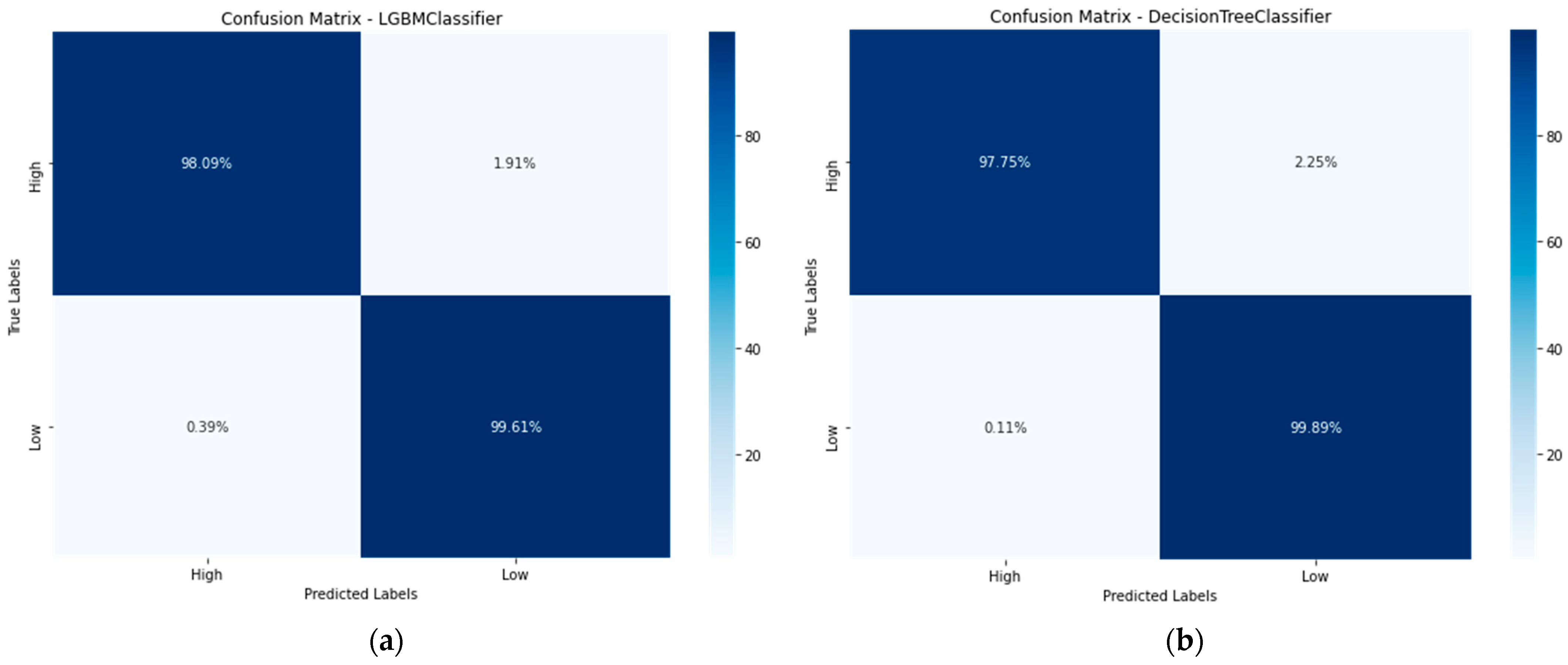
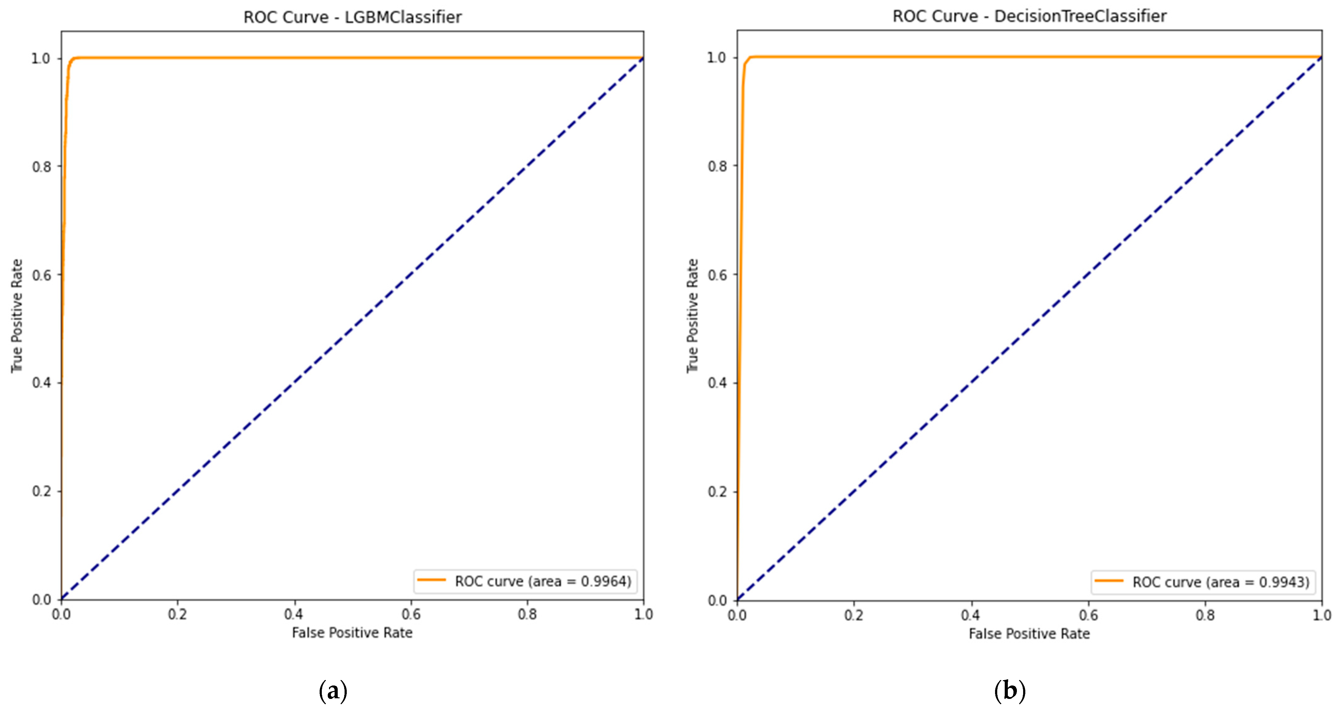
• Performance Metrics Assessment: Key performance metrics, such as those mentioned in Step 5, are reviewed to assess the performance of the models across the different wear categories. These metrics help understand the models’ abilities to correctly predict high and low wear conditions and their robustness against false predictions.
• Model Selection Based on Practical Implications: The top model is selected based on its performance and practicality in deployment. The latter considers several factors, including the model’s ability to minimize both FN and FP rates, the impact of these rates on maintenance operations and safety, and the overall cost-effectiveness of implementing the model. In this context, an FN occurs when the model predicts a ‘Low’ wear condition when the actual label is ‘High.’ This case is particularly concerning because failing to identify a high-wear condition could lead to undetected brake wear, potentially compromising safety. Therefore, minimizing the FN rate is key to detecting and promptly addressing all significant wear instances. An FP, on the other hand, happens when the model predicts a ‘High’ wear condition when the actual label is ‘Low.’ While this does not pose a direct safety risk, it can lead to unnecessary inspections and maintenance work, increasing operational costs and causing potential downtime. Minimizing the FP rate is important to maintain cost-effectiveness and operational efficiency. This analysis helps select the model that best balances accuracy with practical deployment considerations, ensuring that it can be effectively leveraged by existing aircraft maintenance systems.

4.7. Step 7: Model Interpretability and Explainability

This step focuses on identifying which features most strongly influence the predictions of the top-performing models. Analyzing the contribution of variables such as operational parameters and environmental conditions to brake wear predictions offers valuable insights into the factors that most critically affect degradation. These findings can inform maintenance planning and guide operational adjustments to enhance brake system longevity.

The models benchmarked in Step 4 are either directly interpretable (e.g., Logistic Regression, Decision Tree) or explainable. For instance, the decision rules of the Decision Tree model are important to understand precisely how predictions are made and how certain features influence outcomes, whereas tree-based ensemble methods (e.g., Random Forest, LGBM) can provide insights into feature importance.

4.8. Step 8: Uncertainty Quantification

Uncertainty quantification informs about confidence levels around the predictions, giving a probabilistic understanding of wear levels rather than a definitive classification. As such, this process involves adjusting the models to output probabilities instead of binary classifications. For instance, instead of merely predicting ‘High’ or ‘Low’ wear, the model outputs a probability distribution across possible wear conditions, which helps in making more informed maintenance decisions under uncertainty. The sources of uncertainty could include variability in wear measurements, inconsistencies in operational conditions, and discrepancies in external factors such as weather data. By accounting for these uncertainties, this method embeds a layer of risk assessment in the predictive maintenance strategy, ensuring that decisions are made considering the confidence in the predictions and their reliability (i.e., consistency and dependability). In other words, the model’s reliability indicates how likely it is to produce accurate and repeatable results under different conditions and over multiple instances.

This eight-step methodology presents a rigorous and systematic approach to classifying the carbon brake wear severity that flights experience in operation. The subsequent section details the results and provides an in-depth discussion regarding their implications.

5. Results and Discussion

This section presents a detailed analysis of the benchmarking results for various ML models used for predicting carbon brake wear. The evaluation emphasizes model performance, selection of the most suitable model for operational deployment based on accuracy and practicality (e.g., minimization of errors to ensure safety and reduce costs), and assessment of the most significant features contributing to brake wear. Additionally, it includes an examination of the uncertainty associated with the predictions.

5.1. Model Performance Evaluation and Selection

Table 6. Top Model Architecture (Fleet).

Model	Best Parameters	Accuracy	Recall	Precision	F1 Score	AUC Score
LGBM	‘learning_rate’: 0.03, ‘max_depth’: 20, ‘n_estimators’: 200, ‘num_leaves’: 62, ‘random_state’: 0	0.9892	0.9885	0.9898	0.9891	0.9964
Decision Tree	‘criterion’: ‘gini’, ‘max_depth’: 3, ‘min_samples_leaf’: 4, ‘min_samples_split’: 2, ‘random_state’: 0	0.9892	0.9882	0.9902	0.9891	0.9943
XGBoost	‘learning_rate’: 0.01, ‘max_depth’: 3, ‘n_estimators’: 100, ‘random_state’: 0	0.9891	0.9880	0.9900	0.9890	0.9960
CatBoost	‘depth’: 10, ‘iterations’: 1000, ‘learning_rate’: 0.1, ‘random_state’: 0	0.9886	0.9882	0.9889	0.9885	0.9963
Random Forest	‘criterion’: ‘gini’, ‘max_depth’: 30, ‘min_samples_leaf’: 1, ‘min_samples_split’: 4, ‘n_estimators’: 100, ‘random_state’: 0	0.9871	0.9868	0.9871	0.9870	0.9945
SVC	‘C’: 1, ‘gamma’: ‘scale’, ‘kernel’: ‘linear’, ‘probability’: True, ‘random_state’: 0	0.9837	0.9833	0.9838	0.9835	0.9815
Logistic Regression	‘C’: 100, ‘max_iter’: 100, ‘random_state’: 0, ‘solver’: ‘lbfgs’	0.9805	0.9802	0.9804	0.9803	0.9829
KNN	‘metric’: ‘manhattan’, ‘n_neighbors’: 10, ‘weights’: ‘uniform’	0.8218	0.8091	0.8411	0.8136	0.9041

presents a comparison of ML models evaluated for the task of classifying high versus low brake wear, using a linear spline interpolation approach to generate labels. For each model, the table lists the hyperparameters and corresponding values that yielded the best performance, as determined through grid search optimization.

The LGBM classifier stands out as the best performer, achieving the highest scores (in terms of Accuracy, Recall, F1 Score, and AUC) with a learning rate of 0.03, a maximum depth of 20, the number of estimators set to 200, and the number of leaves set to 62. The Decision Tree classifier exhibits the same accuracy of 98.92% and the highest precision of 99.02%. The CatBoost, Random Forest, SVC, and Logistic Regression models also show robustness across metrics, with each score greater than 98%. In contrast, KNN shows notably lower scores across all metrics.

The grid search results for the binary classification case (‘High’ vs. ‘Low’ brake wear), utilizing 5-fold cross-validation for a range of interpolation methods, are detailed in

Table A1. Grid Search with 5-Fold Cross-Validation Results for Binary Classification (High vs. Low Brake Wear) for Various Interpolation Methods. Bold values indicate the best scores achieved.

Interpolation Method	Model	Best Parameters	Accuracy	Recall	Precision	F1 Score	AUC Score
Slinear	LGBM	{‘learning_rate’: 0.03, ‘max_depth’: 20, ‘n_estimators’: 200, ‘num_leaves’: 62, ‘random_state’: 0}	0.9892	0.9885	0.9898	0.9891	0.9964
	Decision Tree	{‘criterion’: ‘gini’, ‘max_depth’: 3, ‘min_samples_leaf’: 4, ‘min_samples_split’: 2, ‘random_state’: 0}	0.9892	0.9882	0.9902	0.9891	0.9943
	XGBoost	{‘learning_rate’: 0.01, ‘max_depth’: 3, ‘n_estimators’: 100, ‘random_state’: 0}	0.9891	0.9880	0.9900	0.9890	0.9960
	CatBoost	{‘depth’: 10, ‘iterations’: 1000, ‘learning_rate’: 0.1, ‘random_state’: 0}	0.9886	0.9882	0.9889	0.9885	0.9963
	Random Forest	{‘criterion’: ‘gini’, ‘max_depth’: 30, ‘min_samples_leaf’: 1, ‘min_samples_split’: 4, ‘n_estimators’: 100, ‘random_state’: 0}	0.9871	0.9868	0.9871	0.9870	0.9945
	SVC	{‘C’: 1, ‘gamma’: ‘scale’, ‘kernel’: ‘linear’, ‘probability’: True, ‘random_state’: 0}	0.9837	0.9833	0.9838	0.9835	0.9815
	Logistic Regression	{‘C’: 100, ‘max_iter’: 100, ‘random_state’: 0, ‘solver’: ‘lbfgs’}	0.9805	0.9802	0.9804	0.9803	0.9829
	KNN	{‘metric’: ‘manhattan’, ‘n_neighbors’: 10, ‘weights’: ‘uniform’}	0.8218	0.8091	0.8411	0.8136	0.9041
PCHP	CatBoost	{‘depth’: 4, ‘iterations’: 500, ‘learning_rate’: 0.01, ‘random_state’: 0}	0.9883	0.9876	0.9888	0.9882	0.9961
	Decision Tree	{‘criterion’: ‘gini’, ‘max_depth’: 3, ‘min_samples_leaf’: 4, ‘min_samples_split’: 2, ‘random_state’: 0}	0.9875	0.9867	0.9882	0.9874	0.9943
	XGBoost	{‘learning_rate’: 0.01, ‘max_depth’: 3, ‘n_estimators’: 100, ‘random_state’: 0}	0.9872	0.9864	0.9879	0.9871	0.9957
	LGBM	{‘learning_rate’: 0.03, ‘max_depth’: -1, ‘n_estimators’: 200, ‘num_leaves’: 62, ‘random_state’: 0}	0.9870	0.9862	0.9878	0.9869	0.9965
	Random Forest	{‘criterion’: ‘entropy’, ‘max_depth’: None, ‘min_samples_leaf’: 2, ‘min_samples_split’: 6, ‘n_estimators’: 100, ‘random_state’: 0}	0.9863	0.9861	0.9863	0.9862	0.9944
	SVC	{‘C’: 1, ‘gamma’: ‘scale’, ‘kernel’: ‘linear’, ‘probability’: True, ‘random_state’: 0}	0.9837	0.9833	0.9838	0.9835	0.9814
	Logistic Regression	{‘C’: 100, ‘max_iter’: 100, ‘random_state’: 0, ‘solver’: ‘saga’}	0.9818	0.9816	0.9817	0.9817	0.9822
	KNN	{‘metric’: ‘manhattan’, ‘n_neighbors’: 10, ‘weights’: ‘uniform’}	0.7846	0.7709	0.8108	0.7730	0.8804
Spline Order 1	CatBoost	{‘depth’: 4, ‘iterations’: 500, ‘learning_rate’: 0.01, ‘random_state’: 0}	0.9349	0.9356	0.9338	0.9345	0.9770
	LGBM	{‘learning_rate’: 0.01, ‘max_depth’: 3, ‘n_estimators’: 100, ‘num_leaves’: 15, ‘random_state’: 0}	0.9341	0.9348	0.9330	0.9337	0.9610
	XGBoost	{‘learning_rate’: 0.01, ‘max_depth’: 3, ‘n_estimators’: 100, ‘random_state’: 0}	0.9341	0.9348	0.9330	0.9337	0.9609
	Decision Tree	{‘criterion’: ‘gini’, ‘max_depth’: 3, ‘min_samples_leaf’: 1, ‘min_samples_split’: 2, ‘random_state’: 0}	0.9301	0.9311	0.9290	0.9298	0.9517
	KNN	{‘metric’: ‘minkowski’, ‘n_neighbors’: 10, ‘weights’: ‘uniform’}	0.9256	0.9271	0.9246	0.9253	0.9588
	Random Forest	{‘criterion’: ‘entropy’, ‘max_depth’: 3, ‘min_samples_leaf’: 4, ‘min_samples_split’: 2, ‘n_estimators’: 500, ‘random_state’: 0}	0.9156	0.9188	0.9157	0.9155	0.9664
	Logistic Regression	{‘C’: 0.01, ‘max_iter’: 100, ‘random_state’: 0, ‘solver’: ‘liblinear’}	0.9142	0.9175	0.9144	0.9140	0.9480
	SVC	{‘C’: 0.01, ‘gamma’: ‘auto’, ‘kernel’: ‘rbf’, ‘probability’: True, ‘random_state’: 0}	0.9134	0.9169	0.9138	0.9132	0.9266
Spline Order 3	CatBoost	{‘depth’: 4, ‘iterations’: 500, ‘learning_rate’: 0.01, ‘random_state’: 0}	0.9064	0.9040	0.9062	0.9050	0.9653
	KNN	{‘metric’: ‘minkowski’, ‘n_neighbors’: 10, ‘weights’: ‘uniform’}	0.8993	0.8975	0.8984	0.8979	0.9508
	XGBoost	{‘learning_rate’: 0.01, ‘max_depth’: 3, ‘n_estimators’: 100, ‘random_state’: 0}	0.8944	0.8918	0.8939	0.8928	0.9515
	LGBM	{‘learning_rate’: 0.01, ‘max_depth’: 3, ‘n_estimators’: 100, ‘num_leaves’: 15, ‘random_state’: 0}	0.8933	0.8907	0.8929	0.8917	0.9515
	Decision Tree	{‘criterion’: ‘gini’, ‘max_depth’: 3, ‘min_samples_leaf’: 4, ‘min_samples_split’: 2, ‘random_state’: 0}	0.8854	0.8824	0.8850	0.8836	0.9299
	Random Forest	{‘criterion’: ‘entropy’, ‘max_depth’: 3, ‘min_samples_leaf’: 1, ‘min_samples_split’: 4, ‘n_estimators’: 200, ‘random_state’: 0}	0.8702	0.8721	0.8684	0.8694	0.9492
	Logistic Regression	{‘C’: 0.001, ‘max_iter’: 100, ‘random_state’: 0, ‘solver’: ‘lbfgs’}	0.8678	0.8701	0.8661	0.8670	0.9147
	SVC	{‘C’: 0.01, ‘gamma’: ‘auto’, ‘kernel’: ‘rbf’, ‘probability’: True, ‘random_state’: 0}	0.8675	0.8697	0.8658	0.8667	0.9006
Spline Order 5	CatBoost	{‘depth’: 4, ‘iterations’: 1000, ‘learning_rate’: 0.01, ‘random_state’: 0}	0.9182	0.9175	0.9171	0.9173	0.9710
	XGBoost	{‘learning_rate’: 0.03, ‘max_depth’: 3, ‘n_estimators’: 400, ‘random_state’: 0}	0.9176	0.9172	0.9163	0.9167	0.9720
	KNN	{‘metric’: ‘minkowski’, ‘n_neighbors’: 10, ‘weights’: ‘uniform’}	0.9001	0.8988	0.8991	0.8989	0.9481
	LGBM	{‘learning_rate’: 0.01, ‘max_depth’: 3, ‘n_estimators’: 100, ‘num_leaves’: 15, ‘random_state’: 0}	0.8882	0.8894	0.8864	0.8874	0.9517
	Decision Tree	{‘criterion’: ‘gini’, ‘max_depth’: 3, ‘min_samples_leaf’: 1, ‘min_samples_split’: 2, ‘random_state’: 0}	0.8773	0.8782	0.8754	0.8764	0.9286
	Random Forest	{‘criterion’: ‘entropy’, ‘max_depth’: 3, ‘min_samples_leaf’: 1, ‘min_samples_split’: 2, ‘n_estimators’: 200, ‘random_state’: 0}	0.8510	0.8509	0.8489	0.8497	0.9414
	SVC	{‘C’: 0.1, ‘gamma’: ‘scale’, ‘kernel’: ‘sigmoid’, ‘probability’: True, ‘random_state’: 0}	0.8427	0.8428	0.8407	0.8415	0.8482
	Logistic Regression	{‘C’: 0.001, ‘max_iter’: 100, ‘random_state’: 0, ‘solver’: ‘liblinear’}	0.8426	0.8426	0.8405	0.8413	0.9131

of Appendix A. In general, ensemble models that combine multiple individual predictions outperform the single estimator models [61,62,63,64].

Table A2. Grid Search with 5-Fold Cross-Validation Results for Binary Classification (High vs. Low/Medium Brake Wear) for Various Interpolation Methods. Bold values indicate the best scores achieved.

Interpolation Method	Model	Best Parameters	Accuracy	Recall	Precision	F1 Score	AUC Score
Slinear	Random Forest	{‘class_weight’: ‘balanced_subsample’, ‘criterion’: ‘gini’, ‘max_depth’: None, ‘min_samples_leaf’: 2, ‘min_samples_split’: 6, ‘n_estimators’: 100, ‘random_state’: 0}	0.9305	0.9172	0.9164	0.9168	0.9742
	CatBoost	{‘auto_class_weights’: ‘Balanced’, ‘depth’: 4, ‘iterations’: 500, ‘learning_rate’: 0.01, ‘random_state’: 0}	0.9258	0.9291	0.9028	0.9141	0.9797
	Decision Tree	{‘class_weight’: ‘balanced’, ‘criterion’: ‘entropy’, ‘max_depth’: 5, ‘min_samples_leaf’: 1, ‘min_samples_split’: 2, ‘random_state’: 0}	0.9255	0.9237	0.9042	0.9130	0.9778
	XGBoost	{‘learning_rate’: 0.01, ‘max_delta_step’: 1, ‘max_depth’: 3, ‘n_estimators’: 100, ‘random_state’: 0, ‘scale_pos_weight’: 1}	0.9243	0.8896	0.9266	0.9054	0.9725
	LGBM	{‘class_weight’: ‘balanced’, ‘learning_rate’: 0.01, ‘max_depth’: 3, ‘n_estimators’: 300, ‘num_leaves’: 15, ‘random_state’: 0}	0.9017	0.9222	0.8744	0.8901	0.9790
	Logistic Regression	{‘C’: 100, ‘class_weight’: ‘balanced’, ‘max_iter’: 100, ‘random_state’: 0, ‘solver’: ‘lbfgs’}	0.9004	0.9136	0.8727	0.8875	0.9603
	SVC	{‘C’: 10, ‘class_weight’: ‘balanced’, ‘gamma’: ‘scale’, ‘kernel’: ‘linear’, ‘probability’: True, ‘random_state’: 0}	0.8846	0.9115	0.8581	0.8728	0.9622
	KNN	{‘metric’: ‘euclidean’, ‘n_neighbors’: 10, ‘weights’: ‘uniform’}	0.7529	0.7210	0.7081	0.7133	0.7896
PCHIP	CatBoost	{‘auto_class_weights’: ‘Balanced’, ‘depth’: 4, ‘iterations’: 500, ‘learning_rate’: 0.01, ‘random_state’: 0}	0.9078	0.9260	0.8817	0.8970	0.9740
	Random Forest	{‘class_weight’: ‘balanced_subsample’, ‘criterion’: ‘gini’, ‘max_depth’: 10, ‘min_samples_leaf’: 4, ‘min_samples_split’: 2, ‘n_estimators’: 100, ‘random_state’: 0}	0.9072	0.9260	0.8811	0.8964	0.9645
	LGBM	{‘class_weight’: ‘balanced’, ‘learning_rate’: 0.01, ‘max_depth’: 3, ‘n_estimators’: 300, ‘num_leaves’: 15, ‘random_state’: 0}	0.9069	0.9267	0.8808	0.8962	0.9737
	Decision Tree	{‘class_weight’: ‘balanced’, ‘criterion’: ‘entropy’, ‘max_depth’: 3, ‘min_samples_leaf’: 1, ‘min_samples_split’: 2, ‘random_state’: 0}	0.9069	0.9267	0.8808	0.8962	0.9700
	Logistic Regression	{‘C’: 100, ‘class_weight’: ‘balanced’, ‘max_iter’: 100, ‘random_state’: 0, ‘solver’: ‘lbfgs’}	0.8921	0.9150	0.8660	0.8808	0.9558
	SVC	{‘C’: 1, ‘class_weight’: ‘balanced’, ‘gamma’: ‘scale’, ‘kernel’: ‘linear’, ‘probability’: True, ‘random_state’: 0}	0.8866	0.9130	0.8612	0.8755	0.9578
	XGBoost	{‘learning_rate’: 0.01, ‘max_delta_step’: 1, ‘max_depth’: 4, ‘n_estimators’: 100, ‘random_state’: 0, ‘scale_pos_weight’: 2.03}	0.8957	0.8280	0.9312	0.8609	0.9691
Spline Order 1	XGBoost	{‘learning_rate’: 0.01, ‘max_delta_step’: 1, ‘max_depth’: 3, ‘n_estimators’: 200, ‘random_state’: 0, ‘scale_pos_weight’: 1}	0.9024	0.9104	0.8719	0.8868	0.9509
	CatBoost	{‘auto_class_weights’: ‘Balanced’, ‘depth’: 4, ‘iterations’: 500, ‘learning_rate’: 0.01, ‘random_state’: 0}	0.9013	0.9138	0.8704	0.8864	0.9581
	LGBM	{‘class_weight’: ‘balanced’, ‘learning_rate’: 0.01, ‘max_depth’: 3, ‘n_estimators’: 100, ‘num_leaves’: 15, ‘random_state’: 0}	0.8894	0.9060	0.8578	0.8741	0.9476
	Decision Tree	{‘class_weight’: ‘balanced’, ‘criterion’: ‘gini’, ‘max_depth’: 3, ‘min_samples_leaf’: 1, ‘min_samples_split’: 2, ‘random_state’: 0}	0.8874	0.9041	0.8557	0.8720	0.9334
	Random Forest	{‘class_weight’: ‘balanced_subsample’, ‘criterion’: ‘entropy’, ‘max_depth’: 3, ‘min_samples_leaf’: 1, ‘min_samples_split’: 4, ‘n_estimators’: 100, ‘random_state’: 0}	0.8770	0.9008	0.8461	0.8621	0.9453
	Logistic Regression	{‘C’: 0.001, ‘class_weight’: ‘balanced’, ‘max_iter’: 100, ‘random_state’: 0, ‘solver’: ‘lbfgs’}	0.8762	0.9005	0.8454	0.8613	0.9133
	KNN	{‘metric’: ‘minkowski’, ‘n_neighbors’: 10, ‘weights’: ‘uniform’}	0.8782	0.8862	0.8452	0.8601	0.9349
	SVC	{‘C’: 0.01, ‘class_weight’: ‘balanced’, ‘gamma’: ‘auto’, ‘kernel’: ‘sigmoid’, ‘probability’: True, ‘random_state’: 0}	0.8740	0.8990	0.8433	0.8590	0.9068
Spline Order 3	XGBoost	{‘learning_rate’: 0.03, ‘max_delta_step’: 0, ‘max_depth’: 3, ‘n_estimators’: 100, ‘random_state’: 0, ‘scale_pos_weight’: 1}	0.8859	0.8578	0.8589	0.8584	0.9348
	CatBoost	{‘auto_class_weights’: ‘Balanced’, ‘depth’: 4, ‘iterations’: 500, ‘learning_rate’: 0.01, ‘random_state’: 0}	0.8763	0.8677	0.8416	0.8526	0.9400
	LGBM	{‘class_weight’: ‘balanced’, ‘learning_rate’: 0.01, ‘max_depth’: 3, ‘n_estimators’: 100, ‘num_leaves’: 15, ‘random_state’: 0}	0.8628	0.8619	0.8258	0.8395	0.9245
	Decision Tree	{‘class_weight’: ‘balanced’, ‘criterion’: ‘gini’, ‘max_depth’: 3, ‘min_samples_leaf’: 1, ‘min_samples_split’: 2, ‘random_state’: 0}	0.8653	0.8495	0.8293	0.8382	0.9076
	KNN	{‘metric’: ‘minkowski’, ‘n_neighbors’: 10, ‘weights’: ‘uniform’}	0.8416	0.8422	0.8030	0.8167	0.9081
	Random Forest	{‘class_weight’: ‘balanced’, ‘criterion’: ‘entropy’, ‘max_depth’: 3, ‘min_samples_leaf’: 4, ‘min_samples_split’: 2, ‘n_estimators’: 100, ‘random_state’: 0}	0.8328	0.8499	0.7980	0.8117	0.9205
	SVC	{‘C’: 0.01, ‘class_weight’: ‘balanced’, ‘gamma’: ‘auto’, ‘kernel’: ‘sigmoid’, ‘probability’: True, ‘random_state’: 0}	0.8321	0.8497	0.7975	0.8111	0.8672
	Logistic Regression	{‘C’: 0.001, ‘class_weight’: ‘balanced’, ‘max_iter’: 100, ‘random_state’: 0, ‘solver’: ‘liblinear’}	0.8321	0.8492	0.7973	0.8109	0.8836
Spline Order 5	CatBoost	{‘auto_class_weights’: ‘Balanced’, ‘depth’: 4, ‘iterations’: 500, ‘learning_rate’: 0.01, ‘random_state’: 0}	0.8649	0.8590	0.8284	0.8407	0.9323
	XGBoost	{‘learning_rate’: 0.01, ‘max_delta_step’: 1, ‘max_depth’: 3, ‘n_estimators’: 200, ‘random_state’: 0, ‘scale_pos_weight’: 1}	0.8670	0.8334	0.8362	0.8348	0.9213
	LGBM	{‘class_weight’: ‘balanced’, ‘learning_rate’: 0.01, ‘max_depth’: 3, ‘n_estimators’: 100, ‘num_leaves’: 15, ‘random_state’: 0}	0.8544	0.8446	0.8166	0.8280	0.9164
	Decision Tree	{‘class_weight’: ‘balanced’, ‘criterion’: ‘entropy’, ‘max_depth’: 3, ‘min_samples_leaf’: 1, ‘min_samples_split’: 2, ‘random_state’: 0}	0.8503	0.8384	0.8119	0.8228	0.8966
	KNN	{‘metric’: ‘minkowski’, ‘n_neighbors’: 10, ‘weights’: ‘uniform’}	0.8286	0.8284	0.7895	0.8026	0.8978
	Random Forest	{‘class_weight’: ‘balanced_subsample’, ‘criterion’: ‘entropy’, ‘max_depth’: 3, ‘min_samples_leaf’: 1, ‘min_samples_split’: 2, ‘n_estimators’: 100, ‘random_state’: 0}	0.8080	0.8184	0.7720	0.7838	0.9034
	Logistic Regression	{‘C’: 0.001, ‘class_weight’: ‘balanced’, ‘max_iter’: 100, ‘random_state’: 0, ‘solver’: ‘liblinear’}	0.8060	0.8167	0.7701	0.7818	0.8698
	SVC	{‘C’: 0.01, ‘class_weight’: ‘balanced’, ‘gamma’: ‘auto’, ‘kernel’: ‘rbf’, ‘probability’: True, ‘random_state’: 0}	0.8051	0.8171	0.7697	0.7813	0.8434

of Appendix A presents the results of the grid search conducted using 5-fold cross-validation for the binary classification task distinguishing ‘High’ brake wear from the combined ‘Low/Medium’ category. In this scenario, the dataset is unbalanced, with instances labeled as ‘High’ brake wear representing approximately 33% of the dataset, and the remaining data labeled as either ‘Low’ or ‘Medium’ brake wear, combined into a single category and representing approximately 67% of the dataset. As a result, specific adjustments are made to the algorithms’ configurations to address this class imbalance and improve the performance of the ML models. For algorithms such as Logistic Regression, SVC, Decision Tree, Random Forest, and LGBM, the ‘class_weight’ hyperparameter is introduced, which helps the models account for the uneven distribution of classes by adjusting the weight given to each class during training [46,56]. Similarly, for the CatBoost classifier, the ‘auto_class_weights’ parameter is used, which automatically adjusts class weights inversely proportional to their frequencies in the data [57]. Furthermore, the XGBoost classifier receives adjustments by adding two parameters: ‘scale_pos_weight’ and ‘max_delta_step’; the former balances the positive and negative weights, while the latter makes the algorithm’s update step more conservative. These adjustments help improve the classifiers’ abilities to accurately predict in an imbalanced dataset context, ensuring that the models do not become biased towards the majority class [55]. Given the imbalanced nature of the dataset, the F1 score is selected over accuracy as the evaluation metric for the grid search strategy, providing a more nuanced measure of performance by harmonizing the precision and recall and offering a balanced view of both FPs and FNs in each model’s predictions. Additionally, the grid search results with 5-fold cross-validation for the multiclass classification task (‘High’ vs. ‘Medium’ vs. ‘Low’ wear) are presented in

Table A3. Grid Search with 5-Fold Cross-Validation Results for Multiclass Classification (High vs. Medium vs. Low Brake Wear) for Slinear Interpolation Method. Bold values indicate the best scores achieved.

Model	Best Parameters	Accuracy	Recall	Precision	F1 Score	AUC Score
CatBoost	{‘depth’: 4, ‘iterations’: 1000, ‘learning_rate’: 0.01, ‘random_state’: 0}	0.8634	0.8619	0.8651	0.8630	0.9684
Random Forest	{‘criterion’: ‘entropy’, ‘max_depth’: 10, ‘min_samples_leaf’: 4, ‘min_samples_split’: 2, ‘n_estimators’: 100, ‘random_state’: 0}	0.8455	0.8444	0.8478	0.8458	0.9500
LGMB	{‘learning_rate’: 0.01, ‘max_depth’: 3, ‘n_estimators’: 100, ‘num_class’: 3, ‘num_leaves’: 15, ‘objective’: ‘multiclass’, ‘random_state’: 0}	0.8434	0.8394	0.8519	0.8406	0.9625
XGBoost	{‘learning_rate’: 0.01, ‘max_depth’: 3, ‘n_estimators’: 100, ‘num_class’: 3, ‘objective’: ‘multi:softmax’, ‘random_state’: 0}	0.8434	0.8394	0.8518	0.8406	0.9605
Decision Tree	{‘criterion’: ‘entropy’, ‘max_depth’: 3, ‘min_samples_leaf’: 1, ‘min_samples_split’: 2, ‘random_state’: 0}	0.8030	0.8106	0.8042	0.8012	0.9503
Logistic Regression	{‘C’: 100, ‘max_iter’: 300, ‘multi_class’: ‘multinomial’, ‘random_state’: 0, ‘solver’: ‘lbfgs’}	0.7925	0.7928	0.7958	0.7942	0.9300
SVC	{‘C’: 100, ‘gamma’: ‘scale’, ‘kernel’: ‘linear’, ‘probability’: True, ‘random_state’: 0}	0.7840	0.7866	0.7887	0.7871	0.9280
KNN	{‘metric’: ‘euclidean’, ‘n_neighbors’: 10, ‘weights’: ‘uniform’}	0.5466	0.5375	0.5681	0.5386	0.7339

of Appendix A, where the labels are balanced (~33% each).

Acknowledging that the outcomes documented in Table 6, Table A1, Table A2 and Table A3 are derived from features representing the mean of numerical attributes across segments characterized by uniform wear pin values is important. Initially, the dataset is considerably larger, where the features are not averaged over constant wear pin value segments. In the context of binary classification aimed at distinguishing between ‘High’ and ‘Low’ brake wear, the original dataset comprises 359,958 rows. This substantial dataset size poses significant challenges for conventional grid search methods, which are inherently time-consuming and computationally demanding due to their methodical examination of every conceivable combination of hyperparameters [58,59]. To circumvent these obstacles and enhance the efficiency of the model optimization process, HyperOpt is introduced as an alternative to grid search. HyperOpt’s advantage lies in its utilization of Bayesian optimization, which strategically navigates the hyperparameter space, substantially reducing the time and computational resources needed [65]. The application of HyperOpt, through 100 iterations on the original dataset’s features, is detailed in

Table A4. HyperOpt (100 Iterations) Results for Binary Classification (High vs. Low Brake Wear) on Original Numerical Features and Using Slinear Interpolation Method. Bold values indicate the best scores achieved.

Model	Best Parameters	Accuracy	Recall	Precision	F1 Score	AUC Score
LGBM	{‘learning_rate’: 0.0454, ‘max_depth’: 3, ‘n_estimators’: 100, ‘num_leaves’: 32, ‘random_state’: 0}	0.7342	0.7302	0.7312	0.7306	0.7965
CatBoost	{‘depth’: 6, ‘iterations’: 100, ‘learning_rate’: 0.0198, ‘random_state’: 0, ‘verbose’: 0}	0.7334	0.7293	0.7303	0.7298	0.7950
XGBoost	{‘learning_rate’: 0.0373, ‘max_depth’: 3, ‘n_estimators’: 101, ‘random_state’: 0}	0.7330	0.7289	0.7299	0.7293	0.7949
SVC *	{‘C’: 90.9715, ‘gamma’: ‘scale’, ‘kernel’: ‘rbf’, ‘probability’: True, ‘random_state’: 0}	0.7277	0.7223	0.7247	0.7232	0.7858
Random Forest	{‘criterion’: ‘gini’, ‘max_depth’: 6, ‘min_samples_leaf’: 5, ‘min_samples_split’: 3, ‘n_estimators’: 134, ‘random_state’: 0}	0.7172	0.7129	0.7138	0.7133	0.7802
Logistic Regression	{‘C’: 0.0080, ‘max_iter’: 940, ‘random_state’: 0, ‘solver’: ‘saga’}	0.7107	0.7050	0.7074	0.7059	0.7699
KNN	{‘metric’: ‘minkowski’, ‘n_neighbors’: 14, ‘weights’: ‘uniform’}	0.7092	0.7053	0.7057	0.7055	0.7635
Decision Tree	{‘criterion’: ‘entropy’, ‘max_depth’: 3, ‘min_samples_leaf’: 4, ‘min_samples_split’: 7, ‘random_state’: 0}	0.7075	0.6914	0.7145	0.6919	0.7488

* SVC model is trained and tested on 40% of the original data to reduce computing time.

of Appendix A. This systematic yet efficient search for the optimal hyperparameters guarantees practical model tuning, thus improving performance on the extensive dataset without necessitating the significant resource investment typically associated with grid search. Nevertheless, it is observed that the models exhibit subpar performance on the unaltered dataset (i.e., the original dataset where features are not averaged over constant wear pin segments). This result could stem from the inconsistent measurement of the wear pin value, which occurs approximately every ten flights. Consequently, the aircraft may encounter remarkably different operational conditions and environmental factors across these intervals, yet the data remains similarly categorized. Such inconsistencies challenge ML classifiers, complicating their ability to differentiate between categories accurately.

In addition,

Table A5. Grid Search with 5-Fold Cross-Validation and HyperOpt (Using 200 Iterations) Results for Binary Classification (High vs. Low Brake Wear) on Averaged Numerical Features and Using Slinear Interpolation Method. Bold values indicate the best scores achieved.

Hyperparameter Optimization Method	Model	Best Parameters	Accuracy	Recall	Precision	F1 Score	AUC Score
Grid Search (5-fold cross-validation)	LGBM	{‘learning_rate’: 0.03, ‘max_depth’: 20, ‘n_estimators’: 200, ‘num_leaves’: 62, ‘random_state’: 0}	0.9892	0.9885	0.9898	0.9891	0.9964
	Decision Tree	{‘criterion’: ‘gini’, ‘max_depth’: 3, ‘min_samples_leaf’: 4, ‘min_samples_split’: 2, ‘random_state’: 0}	0.9892	0.9882	0.9902	0.9891	0.9943
	XGBoost	{‘learning_rate’: 0.01, ‘max_depth’: 3, ‘n_estimators’: 100, ‘random_state’: 0}	0.9891	0.9880	0.9900	0.9890	0.9960
	CatBoost	{‘depth’: 10, ‘iterations’: 1000, ‘learning_rate’: 0.1, ‘random_state’: 0}	0.9886	0.9882	0.9889	0.9885	0.9963
	Random Forest	{‘criterion’: ‘gini’, ‘max_depth’: 30, ‘min_samples_leaf’: 1, ‘min_samples_split’: 4, ‘n_estimators’: 100, ‘random_state’: 0}	0.9871	0.9868	0.9871	0.9870	0.9945
	SVC	{‘C’: 1, ‘gamma’: ‘scale’, ‘kernel’: ‘linear’, ‘probability’: True, ‘random_state’: 0}	0.9837	0.9833	0.9838	0.9835	0.9815
	Logistic Regression	{‘C’: 100, ‘max_iter’: 100, ‘random_state’: 0, ‘solver’: ‘lbfgs’}	0.9805	0.9802	0.9804	0.9803	0.9829
	KNN	{‘metric’: ‘manhattan’, ‘n_neighbors’: 10, ‘weights’: ‘uniform’}	0.8218	0.8091	0.8411	0.8136	0.9041
HyperOpt (200 iterations)	Decision Tree	{‘criterion’: ‘entropy’, ‘max_depth’: 6, ‘min_samples_leaf’: 3, ‘min_samples_split’: 3, ‘random_state’: 0}	0.9892	0.9884	0.9899	0.9891	0.9945
	LGBM	{‘learning_rate’: 0.0427, ‘max_depth’: 3, ‘n_estimators’: 100, ‘num_leaves’: 76, ‘random_state’: 0}	0.9891	0.9881	0.9900	0.9890	0.9965
	CatBoost	{‘depth’: 9, ‘iterations’: 900, ‘learning_rate’: 0.2651, ‘random_state’: 0, ‘verbose’: 0}	0.9886	0.9881	0.9889	0.9885	0.9959
	XGBoost	{‘learning_rate’: 0.2280, ‘max_depth’: 6, ‘n_estimators’: 396, ‘random_state’: 0}	0.9885	0.9878	0.9890	0.9883	0.9958
	Random Forest	{‘criterion’: ‘entropy’, ‘max_depth’: 5, ‘min_samples_leaf’: 2, ‘min_samples_split’: 6, ‘n_estimators’: 135, ‘random_state’: 0}	0.9860	0.9859	0.9858	0.9859	0.9935
	SVC	{‘C’: 0.8624, ‘gamma’: ‘scale’, ‘kernel’: ‘linear’, ‘probability’: True, ‘random_state’: 0}	0.9837	0.9833	0.9838	0.9835	0.9816
	Logistic Regression	{‘C’: 63.7954, ‘max_iter’: 140, ‘random_state’: 0, ‘solver’: ‘saga’}	0.9803	0.9800	0.9803	0.9801	0.9826
	KNN	{‘metric’: ‘minkowski’, ‘n_neighbors’: 14, ‘weights’: ‘uniform’}	0.8052	0.7924	0.8222	0.7964	0.8871

of Appendix A compares the performance metrics from employing grid search with 5-fold cross-validation alongside HyperOpt, the latter utilizing 200 iterations, for the binary classification task of distinguishing ‘High’ versus ‘Low’ brake wear. This analysis is based on averaged numerical features, with the linear spline interpolation method facilitating data labeling. The results from both fine-tuning methods reveal similarity in performance, again with the LGBM and Decision Tree algorithms standing out as the top two performers. This consistency in performance underscores the robustness of these models across different fine-tuning approaches. Note that the performance metrics reported in Table 6 below and in Table A1, Table A2, Table A3, Table A4 and Table A5 of Appendix A are computed on the held-out test set following hyperparameter tuning using 5-fold cross-validation.

Table 6 shows the comparable performance of the LGBM and the Decision Tree classifiers, both of which achieved the same accuracy as the top-performing models. This tie-in performance is particularly noteworthy given the inherent differences between the two models. The LGBM classifier is an advanced ensemble model that builds the algorithm leaf-wise, often leading to better accuracy with large datasets. It uses gradient boosting frameworks and is designed to be distributed and efficient with faster training speeds and higher efficiency, typically resulting in superior performance for complex classification tasks [56]. On the other hand, the Decision Tree classifier is a single estimator model. This non-parametric algorithm segments the data space into a tree of simple decisions based on individual features. It is easier to interpret due to its transparent logic and the apparent path of decisions leading to a prediction [20,21]. For this dataset and classification task, the Decision Tree’s straightforward approach is as practical as the more complex and computationally intensive methods employed by LGBM. These results indicate that the features present clear and strong signals for the binary classification of brake wear that do not require the additional complexity of an ensemble method like LGBM to achieve high accuracy.

Another performance measurement for ML classification is the confusion matrix. Figure 4 displays the confusion matrices for the binary classification task distinguishing ‘High’ from ‘Low’ brake wear, using both fine-tuned LGBM and Decision Tree classifiers. The diagonal entries show the percentages of correct predictions, whereas the off-diagonal values display the percentages of incorrect predictions. High values on the diagonal elements and low values on the off-diagonal indicate well-performing models [60,61].

Both models perform well in terms of TP and TN rates, which suggests that both are suitable for classifying brake wear. However, the FN rate (i.e., True Label: ‘High’, Predicted Label: ‘Low’) is 17.8% higher for the Decision Tree classifier compared to the LGBM classifier $({\displaystyle \frac{2.25\%-1.91\%}{1.91\%}}\times 100\%)$, which is noteworthy since the consequences of missing ‘High’ brake wear conditions are severe and can impact aircraft safety. The FP rate (i.e., True Label: ‘Low’, Predicted Label: ‘High’) is 71.8% lower for the Decision Tree classifier $({\displaystyle \frac{\left|0.11\%-0.39\%\right|}{0.39\%}}\times 100\%)$, making it a more cost-effective model if false alarms are a concern due to the resulting unnecessary inspections or maintenance work. However, in this case, it is more important to detect as many ‘High’ wear instances as possible to prevent failure (i.e., lower FN rate), so the LGBM Classifier is preferred.

The AUC is another helpful metric that quantifies a model’s ability to differentiate the two classes, with a value closer to 1 being preferable. Figure 5 below presents the ROC curves for both classifiers. While each model effectively differentiates between ‘High’ and ‘Low’ brake wear, the LGBM classifier achieves a slightly higher AUC, exceeding that of the Decision Tree by 0.21%, suggesting a marginally superior ability to rank and separate the two classes. The ROC curves indicate that both models successfully capture meaningful signals that enable effective distinction between ‘High’ and ‘Low’ brake wear.

5.2. Model Explainability/Interpretability

The next step in the analysis involves identifying the most influential features affecting carbon brake wear, using measures such as feature importance scores or decision rules derived from the models.

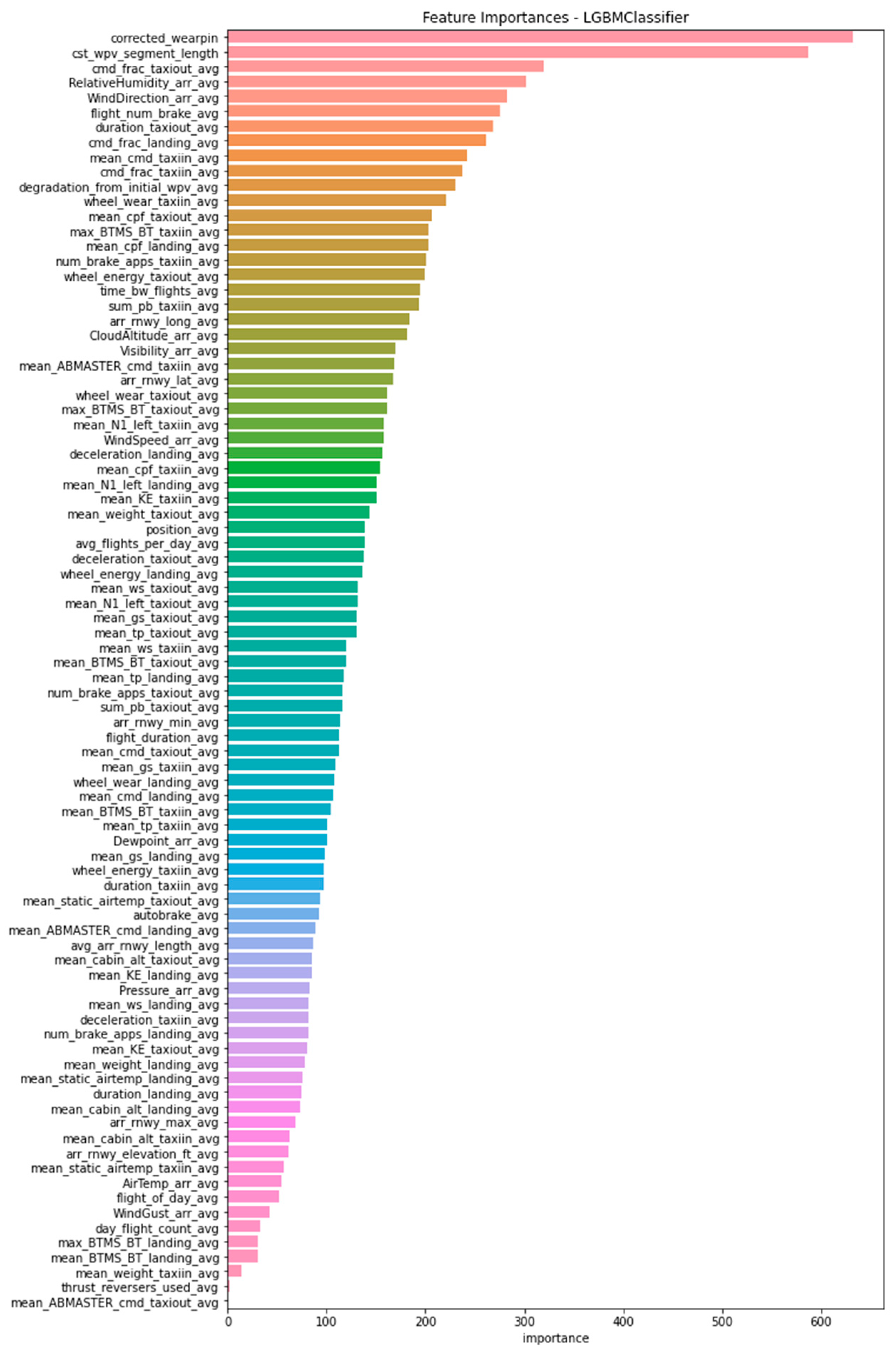
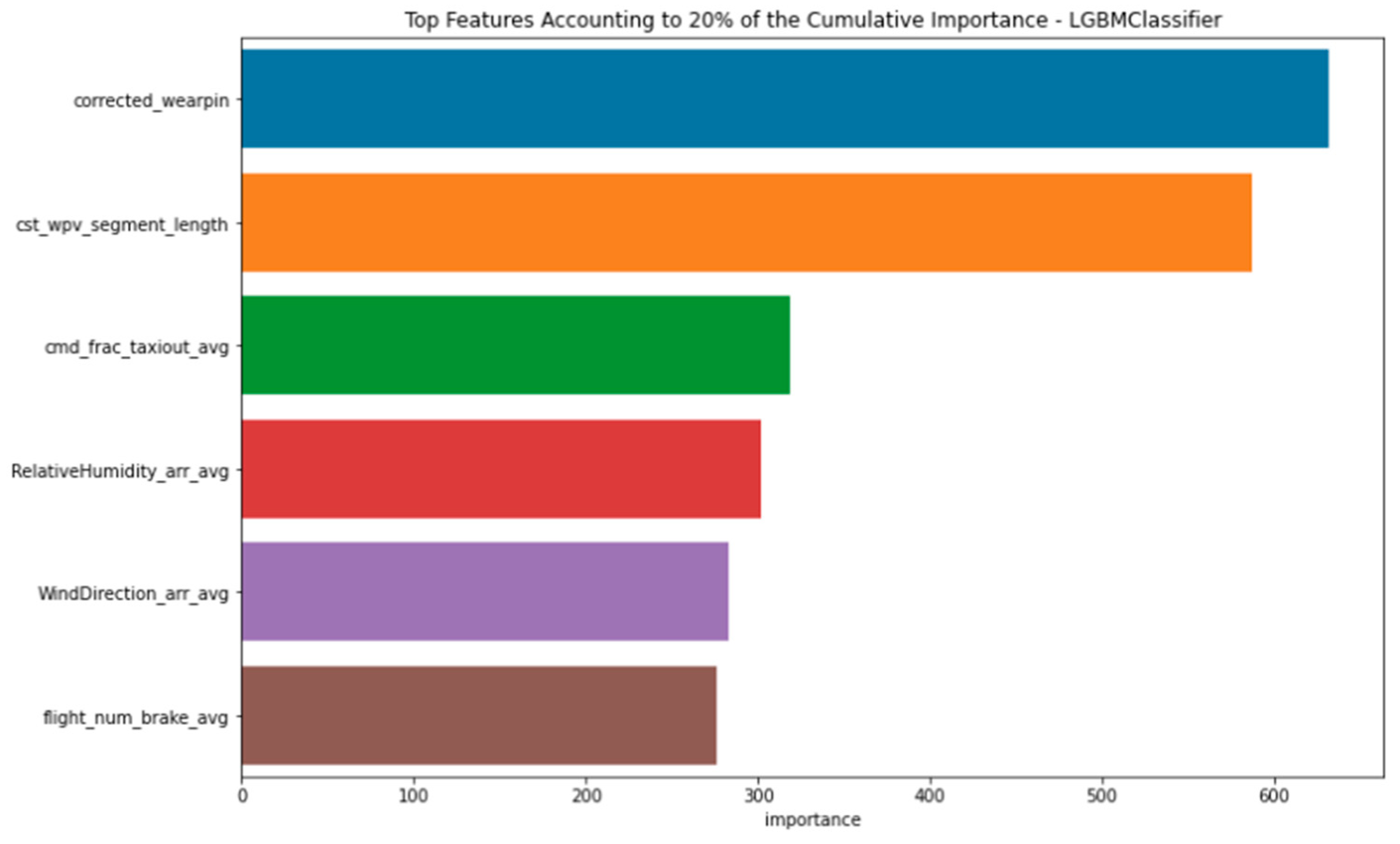
5.2.1. Feature Importance

By default, the LGBM classifier evaluates feature importance based on the number of times each feature is used to split data across all trees in the ensemble. Each branch in a decision tree splits the data into two subsets using the feature that provides the most effective separation, typically based on a criterion such as the Gini index. During training, the LGBM classifier selects features that yield the greatest reduction in the loss function, which quantifies model performance. Features that are chosen more frequently to make impactful splits across the ensemble are deemed more influential [56].

Figure 6 below presents the six features that account for the top 20% of the cumulative, frequency-based feature importance determined by the LGBM classifier. The features, listed from top to bottom, and their relevance to brake degradation are discussed below:

• ‘corrected_wearpin’: This feature corresponds to the original wear pin measurement, corrected during data preprocessing to account for any errors. It is a direct measure of carbon pad thickness and is key to accurately predicting the brake’s remaining life. Additionally, by analyzing changes in the wear pin value over time, it is possible to determine whether the brake wears more, shortly after installation or progressively over time, providing insights into underlying wear patterns and potential issues related to initial installation or long-term usage.
• ‘cst_wvp_segment_length’: This feature captures the number of consecutive flights during which the wear pin value remains constant. An extended period without change may suggest reduced brake wear or efficient brake usage, indicating that the brakes are being applied effectively without excessive or unnecessary engagement. Such patterns are valuable for assessing brake durability across varying operational conditions.
• ‘cmd_frac_taxiout_avg’: This feature represents the average fraction of brake command that the specific brake (out of the eight brakes on the wide-body aircraft) contributes to during the taxi-out phase. This measurement is significant because it reflects the operational load and stress on the brake as the aircraft taxis out of the gate, influencing brake wear rate.
• ‘RelativeHumidity_arr_avg’: This parameter captures the average relative humidity at the arrival airports across the analyzed flights, underscoring the potential influence of environmental conditions on brake performance and the rate at which they degrade.
• ‘WindDirection_arr_avg’: This feature indicates the average wind direction at the airports where the flights arrive, which can also influence aircraft dynamics and braking requirements upon landing. For instance, headwinds or crosswinds might require different braking intensities, thus affecting brake wear.
• ‘flight_num_brake_avg’: This feature captures the average number of flights a specific brake has experienced since its installation. Frequent brake use may lead to faster wear, making this an important factor in predicting when the brake might need maintenance or replacement.

Each feature provides valuable insights into brake usage and environmental exposure, which is essential for accurately predicting carbon brake wear. The remaining features, including those that comprise the remaining 80% of the cumulative importance and their frequency-based importances, are shown in Figure A1 of Appendix A. It is important to note that the feature importance values reported by the LGBM classifier are unitless aggregate scores. These are computed based on the frequency with which each feature is used in tree splits and serve as relative indicators of a feature’s influence on the model’s predictive performance.

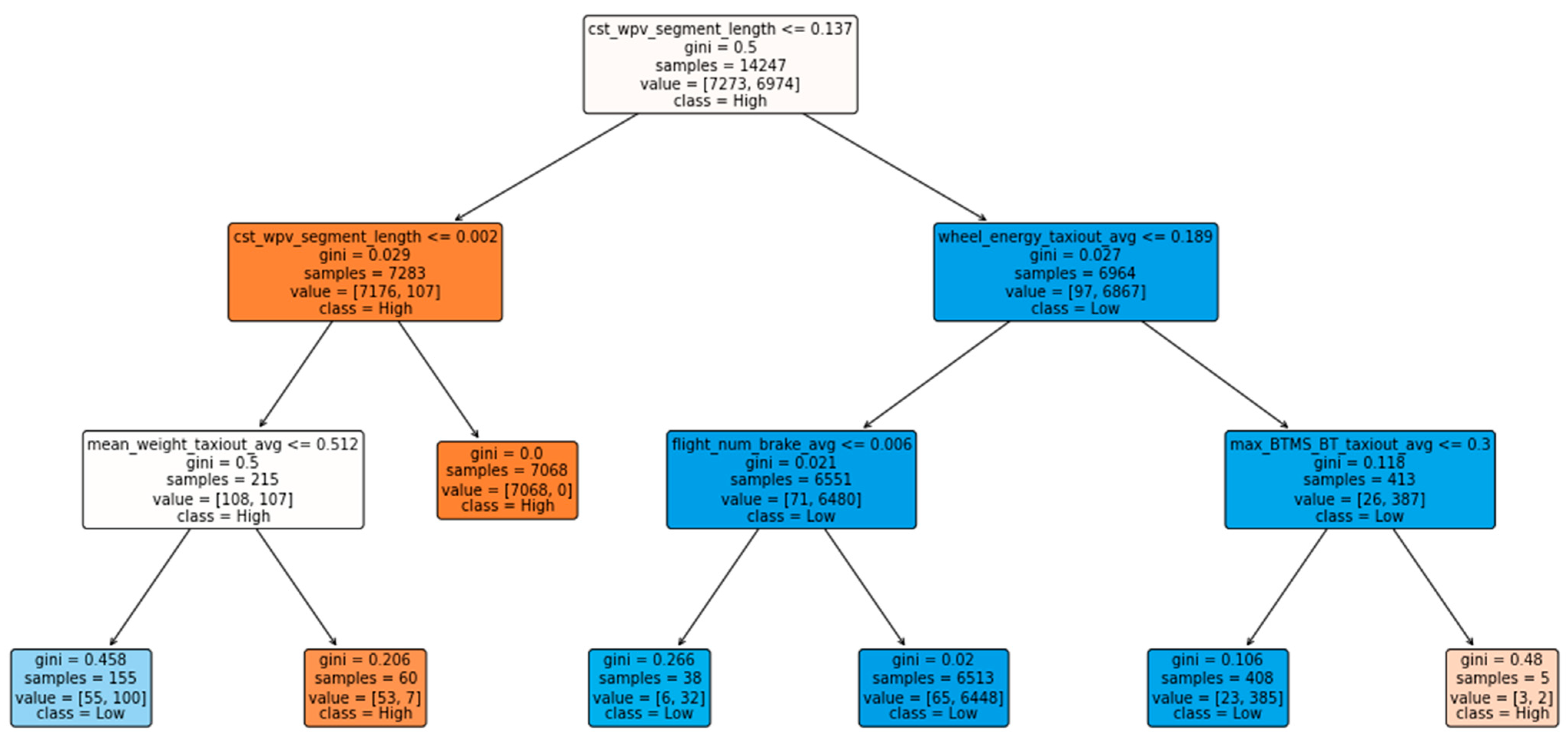
5.2.2. Decision Rules

Unlike the LGBM classifier, which relies on aggregated feature importance scores, the Decision Tree model, also among the top performers, is inherently interpretable due to its transparent structure. Figure 7 below provides the structure of the Decision Tree, where each internal node represents a decision rule applied to a specific feature (e.g., whether a feature’s value is less than or equal to a threshold). The branches denote the outcomes of these tests, guiding the flow along different decision paths. Each path terminates at a leaf node, which corresponds to a final classification outcome derived from the sequence of decision rules applied from the root to that leaf [20,21].

This graphical representation of the Decision Tree classifier offers a clear and straightforward method to trace and understand the logic behind each classification decision, showcasing the model’s rules and criteria for decision-making [20,21]. In this tree:

• Root Node: This is the starting point of the decision tree; the first split in the data is made based on whether the value of ‘cst_wvp_segment_length’ (i.e., the number of flights over which the wear pin value remains constant) is less than or equal to 0.137. Note that all the features were scaled before model training using MinMaxScaler.
• Splitting Nodes: These are the nodes where the branches split off. Each split is based on a condition, with the variables used as conditions for splits in the tree being

  ○

  ‘mean_weight_taxiout_avg’: This variable represents the average aircraft weight during the taxi-out phase. A higher weight during taxi out suggests more significant stress on the braking system due to the increased force required to slow down or stop the heavier aircraft. Therefore, values higher than 0.512 lead to a high-wear classification, which aligns with the intuitive understanding that heavier aircraft exert more wear on the brakes.

  ○

  ‘wheel_energy_taxiout_avg’: This variable measures the average energy at the wheels during taxi out. Lower values of wheel energy, below 0.189 and leading to a low wear classification, indicate less kinetic energy that needs to be dissipated by the brakes. Consequently, less energy at the wheels means the brakes are subjected to lower stress and wear during operations, which correlates with a lower likelihood of significant wear.

• ‘max_BTMS_BT_taxiout_avg’: This variable captures the average maximum brake temperature during taxi out, as measured by the Brake Temperature Monitoring System (BTMS). Lower temperatures, values explicitly less than 0.3, and resulting in a low wear classification imply that the brakes are not overheating, which could cause accelerated wear or lead to carbon oxidation. Cooler brake temperatures may suggest that the braking system is not overused and operates within safe thermal limits, reducing the risk of excessive wear.
  These features used in splits also highlight the significant impact of the taxi-out phase on carbon brake wear, and the selected configuration (max_depth = 3, min_samples_leaf = 4, min_samples_split = 2) constrains the tree’s complexity to improve generalization.
• Gini Index: Each node lists a Gini impurity, which measures how often a random sample would be incorrectly classified according to the label distribution in the subset. A Gini index of 0 indicates perfect purity, meaning all elements in the node belong to a single class.
• Samples: This shows the number of samples sorted into that node after applying the test condition.
• Value: This indicates the distribution of the samples in the classes. For example, value = [7176, 107] means there are 7176 samples of class ‘High’ and 107 samples of class ‘Low’ in this particular node.
• Class: Each node has a class label representing the majority class within that node (i.e., either ‘High’ or ‘Low’ carbon brake wear).

The comparable performance of the LGBM and Decision Tree classifiers highlights both the inherent strength of decision tree-based models for certain datasets and the impact of effective hyperparameter tuning in maximizing model performance. These results underscore the value of evaluating both complex and simpler models during benchmarking, as either can deliver strong performance depending on the characteristics of the dataset and feature space.

5.3. Uncertainty Quantification

The last step of the methodology is concerned with quantifying the uncertainty in the predictions by adjusting models to output the probabilities of belonging to each class (i.e., ‘High’ vs. ‘Low’ wear). Posterior probabilities from the LGBM and Decision Tree models are used to evaluate how confidently each flight set is assigned to a specific brake wear severity category, based on the training data.

5.3.1. LGBM

For classification tasks, the LGBM algorithm converts tree output scores into class probabilities using a logistic (sigmoid) function. These probabilities, which sum to one, represent the model’s confidence in each prediction. Such probabilistic outputs are particularly valuable for evaluating prediction certainty and enabling threshold-based decision strategies in applications like predictive maintenance and risk management. For example, high-confidence predictions (e.g., probability ≥ 0.98) may warrant automated maintenance actions, whereas lower-confidence predictions could be flagged for manual inspection or handled more conservatively.

Table 7. Sample Probabilities of Predictions by LGBM Classifier.

Sample Index	True Label	Predicted Label	Probability of High Wear	Probability of Low Wear
5529	0	0	0.9988	0.0012
4770	0	0	0.9988	0.0012
4718	1	1	0.0013	0.9987
3813	0	0	0.9988	0.0012
1252	1	1	0.0016	0.9984

presents example predictions from the LGBM classifier, where ‘0’ denotes ‘High’ and ‘1’ denotes ‘Low’ wear, along with their associated probabilities.

5.3.2. Decision Tree

The Decision Tree estimates posterior probabilities based on the distribution of class labels among the training samples that reach each leaf node. For a given prediction, the class probabilities are derived from the proportion of training instances at the corresponding leaf. While less granular than those produced by LGBM, these probabilities still convey the model’s relative confidence and offer useful context for interpreting the prediction outcome.

Table 8. Sample Probabilities of Predictions by Decision Tree Classifier.

Sample Index	True Label	Predicted Label	Probability of High Wear	Probability of Low Wear
4348	0	0	1.0000	0.0000
4080	1	1	0.0100	0.9900
1391	1	1	0.0100	0.9900
5380	1	1	0.1579	0.8421
2795	1	1	0.0100	0.9900

provides representative samples from the Decision Tree classifier with predicted labels and associated probabilities.

This process enables stakeholders to compare flights, identify patterns associated with consistent high wear, and derive insights to support predictive maintenance planning and operational improvements. While the focus here is on class probabilities as indicators of prediction confidence, these probabilistic outputs provide a valuable foundation for risk-informed decision-making, such as threshold tuning based on operational tolerance. By leveraging these confidence scores, maintenance actions can be more flexibly aligned with safety priorities and resource constraints.

6. Conclusions and Future Work

This study benchmarks several ML models for classifying carbon brake wear severity using real-world flight data enriched with environmental and airport context from FlightAware^®. The dataset is labeled into distinct wear categories (Low, Medium, or High) using linear spline interpolation of wear pin signals available from the wide-body aircraft fleet. Among the evaluated models, the LGBM classifier demonstrates the strongest performance, achieving high scores across all evaluation metrics (Accuracy (98.92%), Recall (98.85%), F1 Score (98.91%), and AUC (99.64%)) when optimized via grid search. Its effectiveness is attributed to the model’s robust ensemble learning framework and ability to efficiently process the rich, multidimensional dataset.

This work also demonstrates that a simpler, interpretable model can achieve performance comparable to that of a more sophisticated algorithm, provided appropriate hyperparameter tuning. While the LGBM classifier demonstrated the highest overall performance, the Decision Tree classifier achieved nearly identical accuracy and F1 scores despite its significantly lower complexity. This finding underscores an interesting trade-off: while ensemble methods like LGBM yield marginal improvements in predictive performance, they do so at the expense of increased computational complexity and reduced model transparency. In contrast, Decision Trees enable the extraction of interpretable decision rules that can be readily validated by domain experts, an advantage in safety-critical systems where explainability and trust are essential.

The consistent performance across multiple evaluation metrics highlights the reliability and practical applicability of both models in predictive maintenance scenarios, an important factor for scheduling timely interventions, minimizing unexpected failures, and optimizing maintenance costs. These findings underscore the value of evaluating a diverse range of models and tuning strategies, advocating for a balanced selection approach that weighs predictive accuracy, model complexity, interpretability, and operational efficiency. Such considerations are key when deploying ML models in real-world settings, where predictive errors, particularly false negatives, can carry significant safety and cost implications.

From a deployment perspective, the Decision Tree may be more suitable for real-time or resource-constrained environments due to its faster inference speed and lower computational overhead, supporting easier integration into existing airline maintenance systems. While both models achieve similar accuracy, the LGBM classifier is preferred in this study for its superior handling of high-risk misclassifications, specifically cases where ‘High’ wear is misclassified as ‘Low’. This makes it more appropriate for safety-sensitive applications where minimizing critical errors outweighs marginal gains in interpretability. Ultimately, model selection should be guided by the deployment context, system constraints, and the acceptable level of predictive error aligned with operational risk tolerance.

Furthermore, the most influential variables in classifying brake wear are identified through detailed feature importance analysis using the LGBM model. Weather-related features, particularly relative humidity and wind direction, were found to significantly enhance predictive performance. In contrast, the Decision Tree provides transparent decision logic, highlighting operational factors like the taxi-out phase as key contributors to wear. Additionally, posterior probabilities are used to quantify uncertainty, enabling risk-aware maintenance strategies that align with the system’s tolerance for misclassification.

The primary limitation of this study lies in the low resolution and inconsistent reporting frequency of the wear pin signal (recorded to the nearest integer and typically updated only every 10 flights), which restricts the ability to capture fine-grained degradation trends. Moreover, the sparsity of wear pin measurements over long intervals introduces noise due to varying operational and environmental conditions occurring between updates. These unobserved variations weaken the association between inputs and wear labels, thereby limiting the generalizability of the trained models to other aircraft or operational settings. This limitation is particularly consequential for future work aiming to develop supervised regression models that predict the continuous value of brake wear per flight, where higher-resolution data would significantly enhance predictive performance and enable the estimation of brake pad RUL. Incorporating more advanced onboard sensors that record wear pin signals at finer resolution and/or with increased frequency could enable more granular observations and improve the fidelity of wear estimation. Models capable of forecasting exact wear levels per flight, rather than discrete categories, would facilitate more precise maintenance planning and optimized scheduling.

Additionally, while airport-related features are incorporated, the FlightAware^® dataset provides only aggregated values per airport, lacking runway-specific attributes and surface conditions (e.g., wetness, roughness) that can influence braking force and wear. Including more granular runway information in future studies could further improve predictive performance. Moreover, integrating more diverse operational datasets, including those from different aircraft types and airline operations, could enhance model generalizability. Transfer Learning (TL) approaches may also be explored to transfer predictive knowledge across platforms (e.g., from one aircraft type to another). Lastly, enabling real-time data processing and model updating would support adaptive learning as new data becomes available, and inform robust and practical predictive maintenance solutions aligned with evolving operational demands.

References

1. Liu, Z.; Li, Z.; Qin, C.; Shang, Y.; Liu, X. The Review and Development of the Brake System for Civil Aircrafts. In Proceedings of the 2016 IEEE International Conference on Aircraft Utility Systems (AUS), Beijing, China, 10–12 October 2016; IEEE: Piscataway, NJ, USA, 2016. [Google Scholar] [CrossRef]
2. Allen, T.; Miller, T.; Preston, E. Operational Advantages of Carbon Brakes. Aeromagazine 2009, 3, 35. Available online: https://code7700.com/pdfs/operational_advantages_carbon_brakes.pdf (accessed on 5 June 2025).
3. Wang, H. A Survey of Maintenance Policies of Deteriorating Systems. Eur. J. Oper. Res. 2002, 139, 469–489. [Google Scholar] [CrossRef]
4. Zhu, T.; Ran, Y.; Zhou, X.; Wen, Y. A Survey of Predictive Maintenance: Systems, Purposes and Approaches. arXiv 2019, arXiv:1912.07383. [Google Scholar]
5. Kotsiantis, S.B. Supervised Machine Learning: A Review of Classification Techniques. In Emerging Artificial Intelligence Applications in Computer Engineering; Maglogiannis, I.G., Ed.; IOS Press: Amsterdam, The Netherlands, 2007; Volume 160, pp. 3–24. [Google Scholar]
6. Singh, A.; Thakur, N.; Sharma, A. A Review of Supervised Machine Learning Algorithms. In Proceedings of the 2016 3rd International Conference on Computing for Sustainable Global Development (INDIACom), New Delhi, India, 16–18 March 2016; IEEE: New York, NY, USA, 2016. [Google Scholar]
7. Phillips, P.; Diston, D.; Starr, A.; Payne, J.; Pandya, S. A review on the optimisation of aircraft maintenance with application to landing gears. In Engineering Asset Lifecycle Management; Kiritsis, D., Emmanouilidis, C., Koronios, A., Mathew, J., Eds.; Springer: London, UK, 2010; pp. 89–106. [Google Scholar] [CrossRef]
8. Oikonomou, A.; Loutas, T.; Eleftheroglou, N.; Freeman, F.; Zarouchas, D. Remaining Useful Life Prognosis of Aircraft Brakes. Int. J. Progn. Health Manag. 2022, 13, 3072. [Google Scholar] [CrossRef]
9. Hsu, T.-H.; Chang, Y.-J.; Hsu, H.-K.; Chen, T.-T.; Hwang, P.-W. Predicting the Remaining Useful Life of Landing Gear with Prognostics and Health Management (PHM). Aerospace 2022, 9, 462. [Google Scholar] [CrossRef]
10. Travnik, M.; Hansman, R.J. A Data Driven Approach for Predicting Friction-Limited Aircraft Landings. In Proceedings of the AIAA SCITECH 2022 Forum, San Diego, CA, USA, 3–7 January 2022. [Google Scholar] [CrossRef]
11. Steffan, J.J.; Jebadurai, I.J.; Asirvatham, L.G.; Manova, S.; Larkins, J.P. Prediction of Brake Pad Wear Using Various Machine Learning Algorithms. In Recent Trends in Design, Materials and Manufacturing; Singh, M.K., Gautam, R.K., Eds.; Lecture Notes in Mechanical Engineering; Springer: Singapore, 2022; pp. 529–543. [Google Scholar] [CrossRef]
12. Magargle, R.; Johnson, L.; Mandloi, P.; Davoudabadi, P.; Kesarkar, O.; Krishnaswamy, S.; Batteh, J.; Pitchaikani, A. A Simulation-Based Digital Twin for Model-Driven Health Monitoring and Predictive Maintenance of an Automotive Braking System. In Proceedings of the 12th International Modelica Conference, Prague, Czech Republic, 15–17 May 2017; Linköping University Electronic Press: Linköping, Sweden, 2017; pp. 235–244. [Google Scholar] [CrossRef]
13. Küfner, T.; Döpper, F.; Müller, D.; Trenz, A.G. Predictive Maintenance: Using Recurrent Neural Networks for Wear Prognosis in Current Signatures of Production Plants. Int. J. Mech. Eng. Robot. Res. 2021, 10, 583–591. [Google Scholar] [CrossRef]
14. De Martin, A.; Jacazio, G.; Sorli, M. Simulation of Runway Irregularities in a Novel Test Rig for Fully Electrical Landing Gear Systems. Aerospace 2022, 9, 114. [Google Scholar] [CrossRef]
15. Cao, J.; Bao, J.; Yin, Y.; Yao, W.; Liu, T.; Cao, T. Intelligent prediction of wear life of automobile brake pad based on braking conditions. Ind. Lubr. Tribol. 2023, 75, 157–165. [Google Scholar] [CrossRef]
16. Harlapur, C.C.; Kadiyala, P.; Ramakrishna, S. Brake pad wear detection using machine learning. Int. J. Adv. Res. Ideas Innov. Technol. 2019, 5, 498–501. [Google Scholar]
17. Burnaev, E. Time-series classification for industrial applications: A brake pad wear prediction use case. In IOP Conference Series: Materials Science and Engineering, Proceedings of the 4th International Conference on Mechanical, System and Control Engineering, Moscow, Russian, 20–23 June 2020; IOP Publishing: Bristol, UK, 2020; Volume 904, p. 012012. [Google Scholar] [CrossRef]
18. Choudhuri, K.; Shekhar, A. Predicting Brake Pad Wear Using Machine Learning. Engineering Briefs 2020. Available online: https://assets-global.website-files.com/5e73648af0a7112f91aff9af/5f0c473ff3f009253a3c38a9_EB2020-STP-015.pdf (accessed on 5 June 2025).
19. Hearst, M.A.; Dumais, S.T.; Osuna, E.; Platt, J.; Scholkopf, B. Support vector machines. IEEE Intell. Syst. Their Appl. 1998, 13, 18–28. [Google Scholar] [CrossRef]
20. Charbuty, B.T.; Abdulazeez, A.M. Classification Based on Decision Tree Algorithm for Machine Learning. J. Appl. Sci. Technol. Trends 2021, 2, 20–28. [Google Scholar] [CrossRef]
21. Song, Y.-Y.; Lu, Y. Decision tree methods: Applications for classification and prediction. Shanghai Arch. Psychiatry 2015, 27, 130–135. [Google Scholar] [CrossRef]
22. Breiman, L. Random Forests. Mach. Learn. 2001, 45, 5–32. [Google Scholar] [CrossRef]
23. Gunn, S.R. Support Vector Machines for Classification and Regression; Technical Report; Citeseer: Princeton, NJ, USA, 1997; pp. 5–16. [Google Scholar]
24. FlightAware®. About FlightAware®. Available online: https://flightaware.com/about/ (accessed on 5 June 2025).
25. Boeing. Boeing 787 Dreamliner. Available online: https://www.boeing.com/commercial/787/#/family (accessed on 5 June 2025).
26. Zhou, L.; Pan, S.; Wang, J.; Vasilakos, A.V. Machine learning on big data: Opportunities and challenges. Neurocomputing 2017, 237, 350–361. [Google Scholar] [CrossRef]
27. Drone Pilot Ground School. How to Read An Aviation Routine Weather (METAR) Report. Available online: https://www.dronepilotgroundschool.com/reading-aviation-routine-weather-metar-report/ (accessed on 5 June 2025).
28. Gultepe, I.; Sharman, R.; Williams, P.D.; Zhou, B.; Ellrod, G.; Minnis, P.; Trier, S.; Griffin, S. A Review of High Impact Weather for Aviation Meteorology. Pure Appl. Geophys. 2019, 176, 1869–1921. [Google Scholar] [CrossRef]
29. Horne, W.B.; McCarty, J.L.; Tanner, J.A. Some Effects of Adverse Weather Conditions on Performance of Airplane Antiskid Braking Systems. In NASA Technical Note; NASA: Washington, DC, USA, 1976; ISBN NASA TN D-8202. [Google Scholar]
30. FlightAware®. FlightAware® APIs. Available online: https://flightaware.com/commercial/data/ (accessed on 5 June 2025).
31. García, S.; Luengo, J.; Herrera, F. Data Preprocessing in Data Mining, 1st ed.; Springer: Cham, Switzerland, 2015; Volume 72. [Google Scholar] [CrossRef]
32. Kotsiantis, S.B.; Kanellopoulos, D.; Pintelas, P.E. Data preprocessing for supervised learning. Int. J. Comput. Sci. 2006, 1, 111–117. [Google Scholar]
33. Bennett, D.A. How can I deal with missing data in my study? Aust. N. Z. J. Public Health 2001, 25, 464–469. [Google Scholar] [CrossRef]
34. Enders, C.K. Applied Missing Data Analysis, 2nd ed.; Guilford Publications: New York, NY, USA, 2022. [Google Scholar]
35. Birkhoff, G.; Schultz, M.H.; Varga, R.S. Piecewise Hermite interpolation in one and two variables with applications to partial differential equations. Numer. Math. 1968, 11, 232–256. [Google Scholar] [CrossRef]
36. Rabbath, C.A.; Corriveau, D. A comparison of piecewise cubic Hermite interpolating polynomials, cubic splines and piecewise linear functions for the approximation of projectile aerodynamics. Def. Technol. 2019, 15, 741–757. [Google Scholar] [CrossRef]
37. Davis, P.J. Interpolation and Approximation, 1st ed.; Courier Corporation: North Chelmsford, MA, USA, 1975. [Google Scholar]
38. McKinley, S.; Levine, M. Cubic spline interpolation. Coll. Redwoods 1998, 45, 1049–1060. [Google Scholar]
39. Späth, H. One Dimensional Spline Interpolation Algorithms, 1st ed.; A K Peters/CRC Press: New York, NY, USA, 1995. [Google Scholar] [CrossRef]
40. Willmott, C.J.; Matsuura, K. Advantages of the mean absolute error (MAE) over the root mean square error (RMSE) in assessing average model performance. Clim. Res. 2005, 30, 79–82. [Google Scholar] [CrossRef]
41. Blu, T.; Thévenaz, P.; Unser, M. Linear interpolation revitalized. IEEE Trans. Image Process. 2004, 13, 710–719. [Google Scholar] [CrossRef]
42. Hodge, V.; Austin, J. A Survey of Outlier Detection Methodologies. Artif. Intell. Rev. 2004, 22, 85–126. [Google Scholar] [CrossRef]
43. Lee, D.K.; In, J.; Lee, S. Standard deviation and standard error of the mean. Korean J. Anesthesiol. 2015, 68, 220–223. [Google Scholar] [CrossRef] [PubMed]
44. Kwak, S.K.; Kim, J.H. Statistical data preparation: Management of missing values and outliers. Korean J. Anesthesiol. 2017, 70, 407–411. [Google Scholar] [CrossRef] [PubMed]
45. Raju, V.G.; Lakshmi, K.P.; Jain, V.M.; Kalidindi, A.; Padma, V. Study the Influence of Normalization/Transformation Process on the Accuracy of Supervised Classification. In Proceedings of the 2020 Third International Conference on Smart Systems and Inventive Technology (ICSSIT), Tirunelveli, India, 20–22 August 2020; IEEE: Piscataway, NJ, USA, 2020. [Google Scholar] [CrossRef]
46. Pedregosa, F.; Varoquaux, G.; Gramfort, A.; Michel, V.; Thirion, B.; Grisel, O.; Blondel, M.; Prettenhofer, P.; Weiss, R.; Dubourg, V.; et al. Scikit-learn: Machine Learning in Python. J. Mach. Learn. Res. 2011, 12, 2825–2830. [Google Scholar]
47. Singh, D.; Singh, B. Investigating the impact of data normalization on classification performance. Appl. Soft Comput. 2020, 97, 105524. [Google Scholar] [CrossRef]
48. Aly, M. Survey on multiclass classification methods. Neural Netw. 2005, 19, 2. [Google Scholar]
49. Kolo, B. Binary and Multiclass Classification; Lulu.com: Morrisville, NC, USA, 2011. [Google Scholar]
50. Lorena, A.C.; de Carvalho, A.C.P.L.F.; Gama, J.M.P. A review on the combination of binary classifiers in multiclass problems. Artif. Intell. Rev. 2008, 30, 19–37. [Google Scholar] [CrossRef]
51. Jammal, P.; Pinon Fischer, O.J.; Mavris, D.N.; Wagner, G. Predictive Maintenance of Aircraft Braking Systems: A Machine Learning Approach to Clustering Brake Wear Patterns. In Proceedings of the AIAA SciTech 2025 Forum, Orlando, FL, USA, 6–10 January 2025; AIAA: Reston, VA, USA, 2025. [Google Scholar] [CrossRef]
52. Longadge, R.; Dongre, S. Class Imbalance Problem in Data Mining Review. arXiv 2013, arXiv:1305.1707. [Google Scholar] [CrossRef]
53. Dreiseitl, S.; Ohno-Machado, L. Logistic regression and artificial neural network classification models: A methodology review. J. Biomed. Inform. 2002, 35, 352–359. [Google Scholar] [CrossRef] [PubMed]
54. Peterson, L.E. K-nearest neighbor. Scholarpedia 2009, 4, 1883. [Google Scholar] [CrossRef]
55. Chen, T.; Guestrin, C. XGBoost: A Scalable Tree Boosting System. In Proceedings of the 22nd ACM SIGKDD International Conference on Knowledge Discovery and Data Mining, San Francisco, CA, USA, 13–17 August 2016; pp. 785–794. [Google Scholar] [CrossRef]
56. Ke, G.; Meng, Q.; Finley, T.; Wang, T.; Chen, W.; Ma, W.; Ye, Q.; Liu, T.-Y. LightGBM: A Highly Efficient Gradient Boosting Decision Tree. In Proceedings of the Advances in Neural Information Processing Systems, Long Beach, CA, USA, 4–9 December 2017; Guyon, I., Von Luxburg, U., Bengio, S., Wallach, H., Fergus, R., Vishwanathan, S., Garnett, R., Eds.; Curran Associates, Inc.: Red Hook, NY, USA, 2017; Volume 30. Available online: https://proceedings.neurips.cc/paper_files/paper/2017/file/6449f44a102fde848669bdd9eb6b76fa-Paper.pdf (accessed on 5 June 2025).
57. Prokhorenkova, L.; Gusev, G.; Vorobev, A.; Dorogush, A.V.; Gulin, A. CatBoost: Unbiased Boosting with Categorical Features. In Proceedings of the Advances in Neural Information Processing Systems, Montréal, QC, Canada, 3–8 December 2018; Bengio, S., Wallach, H., Larochelle, H., Grauman, K., Cesa-Bianchi, N., Garnett, R., Eds.; Curran Associates, Inc.: Red Hook, NY, USA, 2018; Volume 31. Available online: https://proceedings.neurips.cc/paper_files/paper/2018/file/14491b756b3a51daac41c24863285549-Paper.pdf (accessed on 5 June 2025).
58. Bergstra, J.; Bardenet, R.; Bengio, Y.; Kégl, B. Algorithms for Hyper-Parameter Optimization. In Proceedings of the Advances in Neural Information Processing Systems 24, Granada, Spain, 12–14 December 2011; Shawe-Taylor, J., Zemel, R., Bartlett, P., Pereira, F., Weinberger, K.Q., Eds.; Curran Associates, Inc.: Red Hook, NY, USA, 2011; Volume 24. Available online: https://proceedings.neurips.cc/paper_files/paper/2011/file/86e8f7ab32cfd12577bc2619bc635690-Paper.pdf (accessed on 5 June 2025).
59. Krstajic, D.; Buturovic, L.J.; Leahy, D.E.; Thomas, S. Cross-validation pitfalls when selecting and assessing regression and classification models. J. Cheminform. 2014, 6, 10. [Google Scholar] [CrossRef] [PubMed]
60. Hossin, M.; Sulaiman, M.N. A Review on Evaluation Metrics for Data Classification Evaluations. Int. J. Data Min. Knowl. Manag. Process 2015, 5, 1–11. [Google Scholar] [CrossRef]
61. Lever, J. Classification evaluation: It is important to understand both what a classification metric expresses and what it hides. Nat. Methods 2016, 13, 603–605. [Google Scholar] [CrossRef]
62. Dietterich, T.G. Ensemble Methods in Machine Learning. In Multiple Classifier Systems. MCS 2000. Lecture Notes in Computer Science; Sharkey, A.J.C., Ed.; Springer: Berlin/Heidelberg, Germany, 2000; Volume 1857, pp. 1–15. [Google Scholar] [CrossRef]
63. Zhou, Z.-H. Ensemble Methods: Foundations and Algorithms; CRC Press: Boca Raton, FL, USA, 2025. [Google Scholar]
64. Opitz, D.; Maclin, R. Popular ensemble methods: An empirical study. J. Artif. Intell. Res. 1999, 11, 169–198. [Google Scholar] [CrossRef]
65. Komer, B.; Bergstra, J.; Eliasmith, C. Hyperopt-Sklearn: Automatic Hyperparameter Configuration for Scikit-Learn. In Proceedings of the 13th Python in Science Conference (SciPy 2014), Austin, TX, USA, 6–12 July 2014; pp. 1–7. [Google Scholar]
Figure 1. Methodology Overview.
Aerospace 12 00602 g001
Figure 2. Actual and Interpolated Wear Pin Values Using Linear Spline vs. Flight Number on a Specific Aircraft Brake.
Aerospace 12 00602 g002
Figure 3. Data Splitting Process by Aircraft Variant and Tail Number.
Aerospace 12 00602 g003
Figure 4. Confusion Matrices for Both LGBM Classifier (a) and Decision Tree Classifier (b).
Aerospace 12 00602 g004
Figure 5. ROC Curves for LGBM Classifier (a) and Decision Tree Classifier (b). The solid orange lines represent the model performance, while the blue dotted lines indicate the performance of a random classifier (i.e., no discrimination capability).
Aerospace 12 00602 g005
Figure 6. Features Accounting for the Top 20% of the Cumulative, Frequency-Based Feature Importances (LGBM Classifier).
Aerospace 12 00602 g006
Figure 7. Decision Tree Visualization.
Aerospace 12 00602 g007