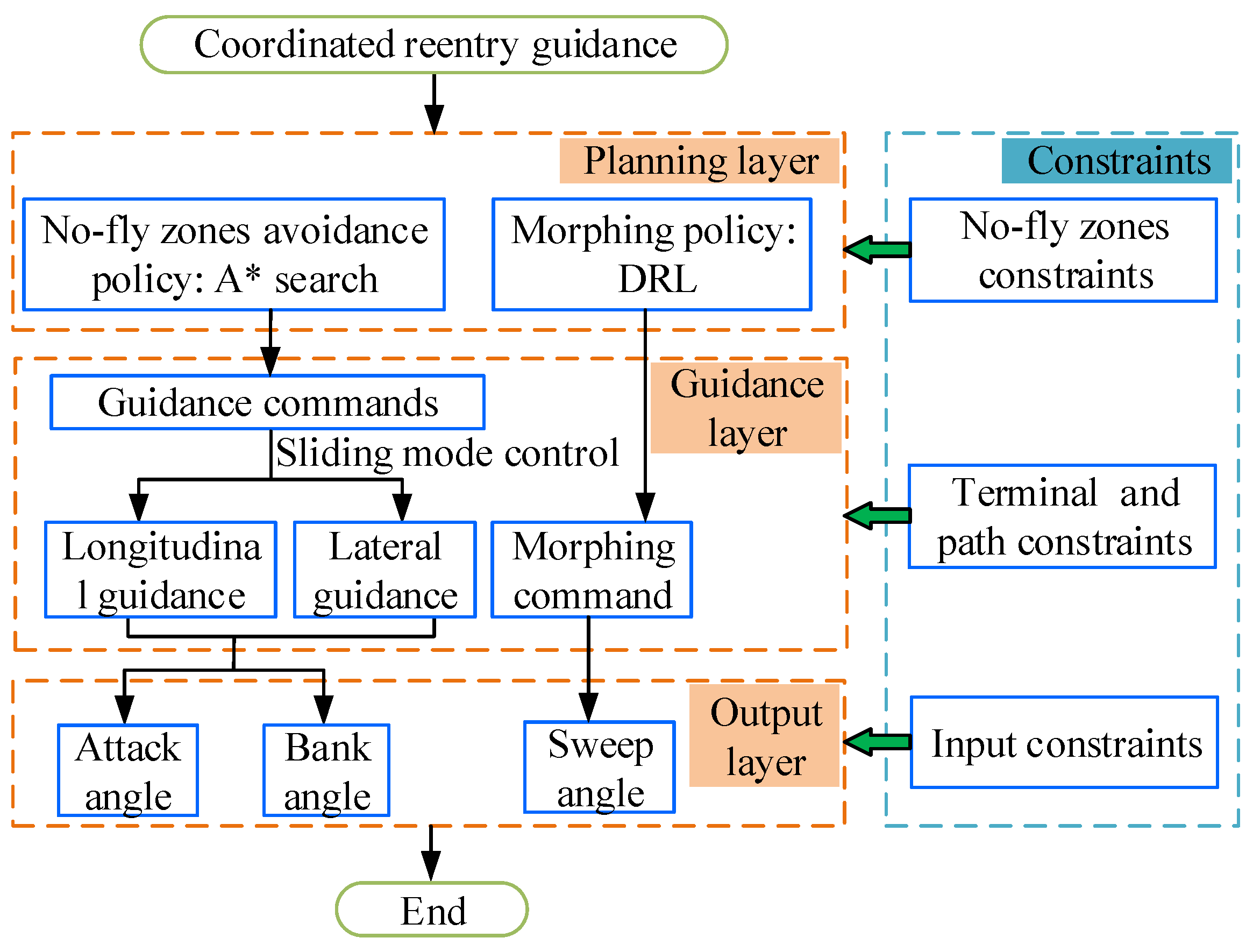
Coordinated Reentry Guidance with A* and Deep Reinforcement Learning for Hypersonic Morphing Vehicles Under Multiple No-Fly Zones

Abstract

Hypersonic morphing vehicles (HMVs), renowned for their adaptive structural reconfiguration and cross-domain maneuverability, confront formidable reentry guidance challenges under multiple no-fly zones, stringent path constraints, and nonlinear dynamics exacerbated by morphing-induced aerodynamic uncertainties. To address these issues, this study proposes a hierarchical framework integrating an A-based energy-optimal waypoint planner, a deep deterministic policy gradient (DDPG)-driven morphing policy network, and a quasi-equilibrium glide condition (QEGC) guidance law with continuous sliding mode control. The A* algorithm generates heuristic trajectories circumventing no-fly zones, reducing the evaluation function by 6.2% compared to greedy methods, while DDPG optimizes sweep angles to minimize velocity loss and terminal errors (0.09 km position, 0.01 m/s velocity). The QEGC law ensures robust longitudinal-lateral tracking via smooth hyperbolic tangent switching. Simulations demonstrate generalization across diverse targets (terminal errors < 0.24 km) and robustness under Monte Carlo deviations (0.263 ± 0.184 km range, −12.7 ± 42.93 m/s velocity). This work bridges global trajectory planning with real-time morphing adaptation, advancing intelligent HMV control. Future research will extend this framework to ascent/dive phases and optimize its computational efficiency for onboard deployment.

1. Introduction

The hypersonic morphing vehicle (HMV), a class of advanced aerospace systems capable of autonomously adjusting their structural configurations and aerodynamic profiles in real time to align with mission-specific requirements and performance objectives, represents a transformative integration of hypersonic flight dynamics and adaptive morphing technology [1,2,3]. By enabling continuous shape transformation, this innovative design paradigm facilitates substantial improvements in aerodynamic efficiency, maneuvering agility, and energy utilization [4,5]. Combining the velocity advantages of hypersonic vehicles with the adaptability of morphing structures, the HMV demonstrates dual capabilities: executing long-endurance, high-maneuverability flights while maintaining the capacity to self-adapt to complex mission demands and cross-domain environments [6]. However, the HMV suffers from complex flight environments, severe force–thermal constraints, and diverse missions in the glide phase. These factors induce significant fluctuations in aerodynamic load distributions and dynamic system parameters, thereby introducing pronounced uncertainties and strong nonlinear behaviors in flight control dynamics, which collectively escalate the complexity of reentry guidance strategies [7].

The reentry guidance of the HMV directs the vehicle with a smooth flight trajectory from the initial reentry point to the terminal area energy management (TAEM) interface at the target precisely without passing through the no-fly zones, provided that the process constraints and terminal constraints are satisfied. Reentry guidance methods include reference trajectory tracking guidance [8,9], predictor–corrector guidance [10], and quasi-equilibrium gliding condition (QEGC) guidance [11,12]. Due to their special reentry trajectory characteristics, the resulting QEGC guidance method is the focus of current research on hypersonic vehicles. By decomposing the reentry guidance into longitudinal and lateral guidance, so that the angle of attack and bank angle are jointly used as control inputs, the QEGC guidance method shows a high control accuracy and excellent robustness in performance with the help of advanced control methods [13]. However, its control of velocity is underactuated and requires the correction of terminal velocity by analytic prediction. Sliding mode control can be used for longitudinal and lateral control in QEGC guidance because of its fast response, good robustness, and simple physical implementation [14,15].

No-fly zones are geographic areas that must be avoided due to air defense threats and political restrictions. Reentry trajectories with no-fly zones require the consideration of complex space constraints. Commonly, no-fly zone avoidance methods include energy-optimal waypoint planning [16], lateral flip logic avoidance [17], the artificial potential field method [18,19], and direct trajectory optimization methods [20,21]. These methods keep away from no-fly zones by planning nominal trajectories. The vehicle is confronted with difficulty flying to the target location when no-fly zones are changed. Search solving is one of the important methods of early artificial intelligence (AI) algorithms. Inspired by the ideas of ground robot and UAV path planning, graph search-based algorithms are also applied to the reentry trajectory planning problem [22,23]. The A* search algorithm in a graph search has an efficient search performance, and it searches feasible paths by setting evaluation functions [24]. The A* algorithm is one of the crucial algorithms for solving the shortest path search problem, capable of exploring based on the spatial information of the problem area and utilizing auxiliary information for heuristic searching [25].

Designing a morphing policy and using morphing ability to improve flight performance are important works of HMV flight control research. Most of the previous studies on HMVs have focused on attitude stability and control under morphing [26,27], while there are relatively few studies on morphing policy. Common morphing policy-solving methods include optimization algorithm [28,29], integrated guidance attitude control solving [30], and reinforcement learning (RL) methods [31,32]. In recent years, with the development of AI represented by RL and deep learning (DL) [33], this also provides new technical directions for exploring the intelligent flight control technology of the HMV [34], and it has been successfully applied to reentry trajectory planning for hypersonic vehicles [35]. Deep reinforcement learning (DRL) techniques are mainly used to solve the continuous decision-making problem of an agent. Consequently, DRL is very suitable for learning the morphing policy of the HMV by continuously interacting with the environment and improving the continuous action policy according to the reward or punishment feedback.

Inspired by the above research, an intelligent coordinated reentry guidance method based on the A* search algorithm and RL is proposed. The intelligent coordinated reentry guidance scheme is shown in Figure 1, and the framework of the reentry guidance is divided into three layers: the planning layer, guidance layer, and output layer. The planning layer includes two tasks. One is to plan the waypoints under multiple no-fly zones through the A* search algorithm and obtain an avoidance policy. The other is learning the morphing policy based on the RL algorithm to obtain the morphing command under different flight states. By combining the A* algorithm with DRL, utilizing A* to tackle the no-fly zone issues and employing DRL for morphing control, we can specifically address the trajectory planning and guidance problems of HMVs under no-fly zone conditions, enhancing the efficiency of online intelligent guidance. The guidance layer receives the waypoints and morphing command from the planning layer and calculates the longitudinal and lateral guidance inputs through the QEGC guidance law by the sliding mode control method. In the output layer, the guidance control input and the morphing command are solved jointly to obtain the corresponding angle of attack, bank angle, and sweep angle, and the input constraints are added to complete the coordinated reentry guidance for the HMV with no-fly zones. The main contributions of this paper are as follows:

• The energy-optimal avoidance reentry trajectory search approach based on A* algorithm, effectively solves the challenge of finding optimal waypoints under the intricate constraints of multiple no-fly zones.
• Leveraging DRL algorithms, an intelligent autonomous morphing policy network for HMVs is trained. This network intelligently utilizes morphing commands to adaptively control terminal velocity, resulting in a significant optimization of reentry guidance performance.
• A QEGC guidance law that relies on a continuous switching sliding mode control is proposed. This approach transforms path constraints into direct guidance input constraints, enabling high-precision guidance with a robust performance.

The rest of this paper is organized as follows: Section 2 establishes the motion models of the HMV. Section 3 presents the no-fly zone avoidance policy. Section 4 describes the QEGC guidance law. The morphing policy based on DRL is discussed in Section 5. The results are tested in Section 6. Finally, Section 7 summarizes the main work.

2. Models of the HMV

2.1. Morphing Mode

The morphing mode of a class of a variable-sweep hypersonic vehicle that we studied is presented in Figure 2. Let the sweep angle of the wing be $\chi$, the morphing of the HMV is the simultaneous change in both wing trailing sweep angles, and $\underset{\_}{\chi }\le \chi \le \overline{\chi }$, where $\overline{\chi }, \underset{\_}{\chi }$ are the upper and lower bounds of the sweep angle, respectively. Define the morphing rate as

$$k={\displaystyle \frac{\chi -\underset{\_}{\chi }}{\overline{\chi }-\underset{\_}{\chi }}}$$

(1)

When $k=0$, the sweep angle is the smallest value $\underset{\_}{\chi }$; when $k=1$, the sweep angle is the largest value $\overline{\chi }$.

2.2. Motion Models

The reentry kinematic equations of the HMV are as follows:

$$\left\{\begin{array}{l}\dot{r}=V\sin \theta \\ \dot{\varphi }=V\cos \theta \cos \sigma /r\\ \dot{\lambda }=-V\cos \theta \sin \sigma /(r\cos \varphi )\end{array}\right.$$

(2)

where $r$ is the geocentric distance, $\varphi$ is the geocentric latitude, and $\lambda$ is the longitude. The three-degree-of-freedom dynamics equations for the HMV in the reentry coordinate system are as follows:

$$a=\left[\begin{array}{c}\dot{V}\\ V\dot{\theta }\\ -V\dot{\sigma }\cos \theta \end{array}\right]={\displaystyle \frac{1}{m}}\left(F_a+G+F_e+F_k+F_T+F_m\right)$$

(3)

where $a$ is the acceleration vector, $V$ is the flight velocity, $\theta$ is the flightpath angle, $\sigma$ is the heading angle measured from the north direction, $m$ is the mass of the HMV, $G=m{\left[\begin{array}{ccc}{g}_V& g_{\theta }& g_{\sigma }\end{array}\right]}^T$ is the Earth’s gravitational force vector, $F_e={\left[\begin{array}{ccc}{F}_{eV}& F_{e\theta }& F_{e\sigma }\end{array}\right]}^T$ is the centrifugal inertia force vector, $F_k={\left[\begin{array}{ccc}{F}_{kx}& F_{ky}& F_{kz}\end{array}\right]}^T$ is the Coriolis inertia force vector, $F_T={\left[\begin{array}{ccc}{F}_{Tx}& F_{Ty}& F_{Tz}\end{array}\right]}^T$ is the implication force resulting from the conversion of the ballistic coordinate system to the reentry coordinate system, and $F_m={\left[\begin{array}{ccc}{F}_{mx}& F_{my}& F_{mz}\end{array}\right]}^T$ is the vector of morphing-added forces due to shape change. The specific expressions of the above force vectors in the reentrant system are given in Ref. [7]. $F_a={\left[\begin{array}{ccc}{F}_{aV}& F_{a\theta }& F_{a\sigma }\end{array}\right]}^T$ is the aerodynamic force vector with the following expressions:

$$F_a=\left[\begin{array}{l}{F}_{aV}\\ F_{a\theta }\\ F_{a\sigma }\end{array}\right]=q{S}_0\left[\begin{array}{c}-C_D\\ C_L\cos \upsilon -C_N\sin \upsilon \\ C_L\sin \upsilon +C_N\cos \upsilon \end{array}\right]$$

(4)

where $q$ is the dynamic pressure, $S_0$ is the reference area, $\upsilon$ is the bank angle, $C_L$ is the lift coefficient, $C_D$ is the drag coefficient, and $C_N$ is the lateral force coefficient. The following part analyzes the effect of morphing on the aerodynamic coefficient of the HMV.

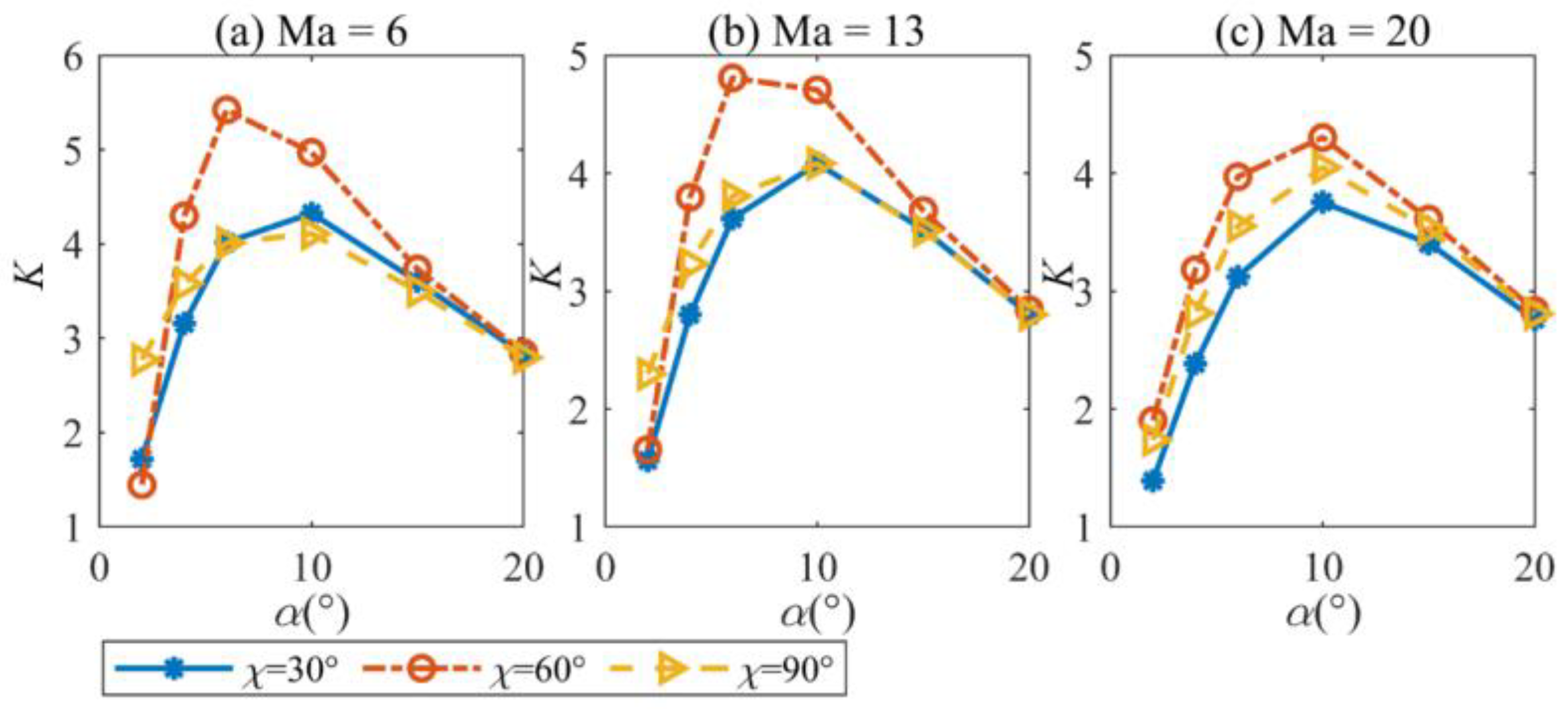
2.3. Effects of Morphing on the Aerodynamic Performance of the HMV

The effects of morphing on the longitudinal aerodynamic coefficient of the HMV in our research are shown in Figure 3, where K is the lift-to-drag ratio. It can be seen that the morphing can significantly change the drag coefficient, lift coefficient, and lift-to-drag ratio of the HMV at a different velocity, so the aerodynamic characteristics of the HMV can be changed by adjusting the sweep angle to achieve the optimal aerodynamic performance to meet the current flight requirements.

2.4. Modeling of Constraints

The constraints of altitude, velocity, range, and heading error need to be satisfied when the vehicle reaches the TAEM interface as follows:

$$\left\{\begin{array}{l}{h}_f=h_T\\ \Delta L_{Rf}=\Delta L_{RT}\\ V_f=V_T\\ \Delta {\sigma }_f\le \Delta {\sigma }_T\end{array}\right.$$

(5)

where $h_f$ is the terminal altitude, $\Delta L_{Rf}$ is the range between the terminal position and the target position, $V_f$ is the terminal velocity, $\Delta {\sigma }_f$ is the terminal heading error, $h_T$ is the target terminal altitude, $\Delta L_{RT}$ is the range between the desired terminal position and the target point, $V_T$ is the target terminal velocity, and $\Delta {\sigma }_T$ is the target terminal heading angle error. The path constraints include heat rate $\dot{Q}$, overload $n$, dynamic pressure $q$ constraints, and QEGC constraints as follows:

$$\left\{\begin{array}{l}\dot{Q}=k_h{\rho }^{0.5}{V}^{3.15}\le {\dot{Q}}_m\\ q={\displaystyle \frac{\rho V^2}{2}}\le q_m\\ n={\displaystyle \frac{\sqrt{D^2+L^2}}{m{g}_0}}\le n_m\\ \dot{\theta }=m(g_0-{\displaystyle \frac{v^2}{r}})\cos \theta -L\cos \upsilon =0\end{array}\right.$$

(6)

where $k_h$ is the heat flow density coefficient, $\rho$ is the atmospheric density, ${\dot{Q}}_{\mathrm{m}}$ is the maximum constraint of the heat flow density, $q_{\mathrm{m}}$ is the maximum constraint value of the dynamic pressure, $D$ and $L$ are the drag and lift force, $g_0$ is the gravitational acceleration, $n_{\mathrm{m}}$ is the maximum constraint value of the overload, and $\dot{\theta }$ is the flightpath angle rate. The bottom surface of no-fly zones is the no-fly circle with the no-fly center as the circular point. In order to avoid the no-fly zones, it is necessary to make the HMV’s position projection on the ground outside the no-fly circle. So,

$$L_{Ri}\ge R_{Zi}$$

(7)

where $L_{Ri}$ is the spherical distance between the position projection and the center of the $i$-th no-fly zones, and $R_{Zi}$ is the radius of the first no-fly circle. Considering attitude stability requirements and the limitations of the morphing and control mechanisms, the attack angle $\alpha$, the bank angle $\upsilon$, and the sweep angle $\chi$ of the HMV need to be limited to a certain range as follows:

$$\left\{\begin{array}{l}{\alpha }_{\min }\le \alpha \le {\alpha }_{\max }\\ {\upsilon }_{\min }\le \upsilon \le {\upsilon }_{\max }\\ {\chi }_{\min }\le \chi \le {\chi }_{\max }\end{array}\right.$$

(8)

where ${\alpha }_{\min }$, ${\upsilon }_{\min }$, and ${\chi }_{\min }$ are the minimum constraint values of the angle of attack, bank angle, and sweep angle, respectively; ${\alpha }_{\max }$, ${\upsilon }_{\max }$, and ${\chi }_{\max }$ are the maximum constraint values of the angle of attack, bank angle, and sweep angle, respectively.

3. No-Fly Zone Avoidance Policy Based on the A* Search Algorithm

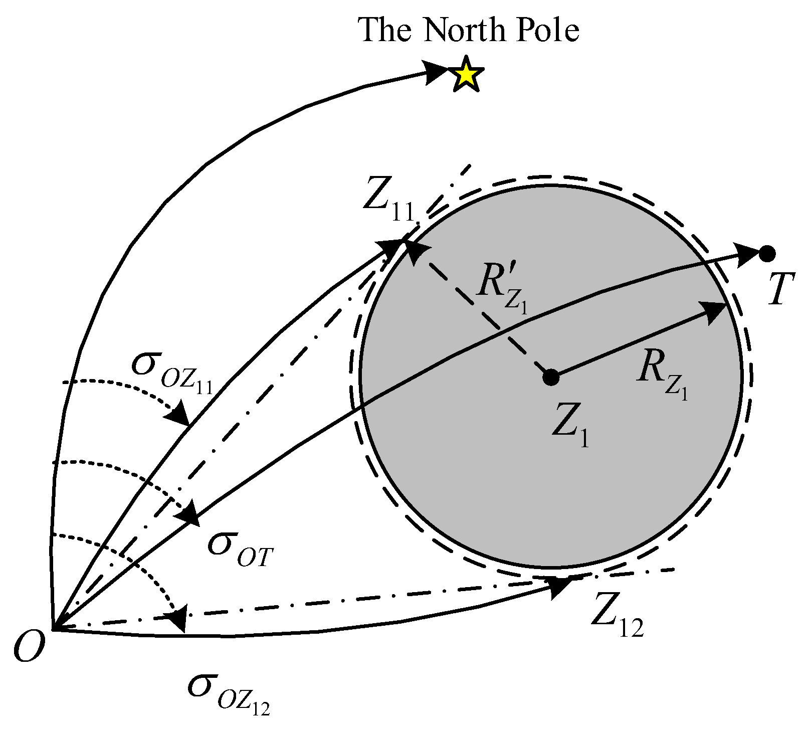
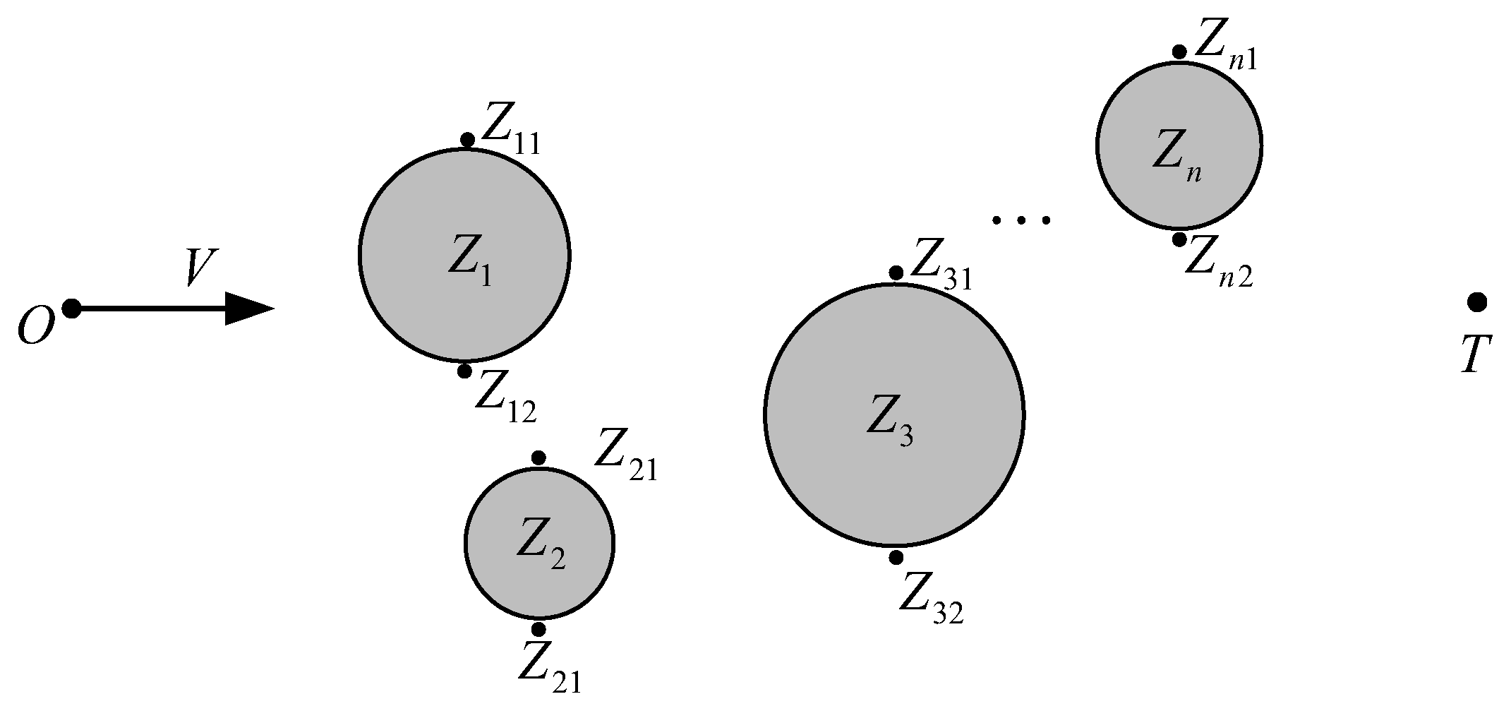
3.1. No-Fly Zone Avoidance Way

As shown in Figure 4, $O$ is the current waypoint of the HMV, $T$ is the next waypoint, $Z_1$ is the center of the circle of the no-fly zones, and $R_{Z_1}$ the radius of the no-fly zones. In order to ensure the safety of the avoidance flight, a safety factor will be added to the radius of the no-fly zones to appropriately expand the no-fly zones as follows:

$$R_{Z_1}^{\prime }=\left(1+\varpi \right)R_{Z_1}$$

(9)

where $\varpi$ is the safety factor; $Z_{11}$ and $Z_{12}$ are the two points of tangency $O$ with respect to the safety radius $R_{Z_1}^{\prime }$ of the no-fly circle $Z_1$; ${\sigma }_{OT}$, ${\sigma }_{O{Z}_{11}}$, and ${\sigma }_{O{Z}_{12}}$ are the azimuthal angles of the trajectory $OT$, $O{Z}_{11}$, and $O{Z}_{12}$, respectively; and the azimuthal angle ${\sigma }_c$ is expressed as

$${\sigma }_c=-\arctan \left({\displaystyle \frac{\sin \left({\lambda }_i-{\lambda }_0\right)}{\cos {\varphi }_0\tan {\varphi }_i-\sin \varphi \cos \left({\lambda }_i-{\lambda }_0\right)}}\right)$$

(10)

where ${\lambda }_0$ and ${\varphi }_0$ are the current longitude and latitude of the HMV, and ${\lambda }_i$ and ${\varphi }_i$ are the target longitude and latitude, respectively. Define $fla{g}_{Z_1}^{OT}$ as the relative position marker between the trajectory $OT$ and the no-fly zone $Z_1$ as follows:

$$fla{g}_{Z_1}^{OT}=\left\{\begin{array}{cc}0& \mathrm{if} {\sigma }_{OT}\in \left[\begin{array}{cc}{\sigma }_{O{Z}_{12}},& {\sigma }_{O{Z}_{12}}\end{array}\right]\\ 1& \mathrm{else}\end{array}\right.$$

(11)

For $N_Z$ no-fly zones: if $\underset{j=1}{\overset{N_z}{\Pi }}fla{g}_{Z_j}^{Z_{ni}{Z}_{\left(n+1\right)i}}=1$, the next waypoint to be flown $Z_{\left(n+1\right)i}$ and the flightpath remains unchanged; if $\underset{j=1}{\overset{N_z}{\Pi }}fla{g}_{Z_j}^{Z_{ni}{Z}_{\left(n+1\right)i}}=0$, the next waypoints have to be adjusted. An optimal set of waypoints need be solved to avoid all the no-fly zones and satisfy the minimum energy consumption of the HMV.

3.2. Design of Evaluation Function

As shown in Figure 5, for the avoidance flight problem under multiple no-fly zones, the HMV starts from the initial position and searches for the next feasible waypoint in the known graph at each current waypoint, so that the flight trajectory can avoid all no-fly zones until it reaches the target position. Finally, the avoidance trajectory with an optimal objective function is obtained. The A* algorithm performs a heuristic search by the evaluation function, which is set to estimate the cost that the current waypoint needs to spend to reach the target. The evaluation function is designed as follows:

$$J\left(n\right)=J_b\left(n\right)+J_{\infty }\left(n\right)$$

(12)

where $n$ denotes the serial number of the node, $J_b\left(n\right)$ is the path’s cost from the initial node $O$ to node $n$, and $J_{\infty }\left(n\right)$ is the estimated value of the cost from node $n$ to the target. The avoidance flight of the HMV with multiple no-fly zones will lead to a large additional energy loss. However, in order to complete the long-range mission to reach the target, the HMV needs to have sufficient energy. Therefore, the additional energy loss for avoidance flight must be considered, and the optimal set of waypoints needs to satisfy the minimum energy consumption as follows:

$$\min J_b\left(n\right)=\min {\displaystyle \sum _{i=2}^N\left|\Delta E_i\right|}$$

(13)

where $N$ denotes the number of waypoints, and $\Delta E_i$ is the additional energy consumed when passing from the $\left(i-1\right)\mathrm{th}$ waypoint to the $i$-th waypoint. To express the additional energy loss directly using the modeling state in Figure 4 and Figure 5, reference [11] treats $\Delta E_i$ as the line of sight azimuth angle increment $\Delta {\sigma }_{ci}$ as

$$J_b\left(n\right)={\displaystyle \sum _{i=1}^{N-1}\left|\Delta {\sigma }_{ci}\right|},\Delta {\sigma }_{ci}={\sigma }_{ci}-{\sigma }_{ci-1}$$

(14)

where ${\sigma }_i$ denotes the line-of-sight azimuth angle when passing the $i$-th waypoint and ${\sigma }_{c0}={\sigma }_0$. The line-of-sight azimuth angle increment $\Delta {\sigma }_{ci}$ between the current waypoint to the target T is regarded as the estimate of the remaining cost as follows:

$$J_{\infty }\left(n\right)=\left|\Delta {\sigma }_{cT}\right|,\Delta {\sigma }_{cT}={\sigma }_{cT}-{\sigma }_{cn}$$

(15)

From Equations (14) and (15), the optimal set of waypoints between multiple no-fly zones is equivalent to the sum of the increments of the line of sight azimuth angle minimized.

3.3. The A*-Based Waypoint Search Algorithm

With the graph modeling and design of the evaluation function, the A*-based multiple no-fly zones waypoint search algorithm is as follows (Algorithm 1):

Algorithm 1: A*-based multiple no-fly zones waypoint search algorithm

Initialization: input the starting position $O$, target $T$, and no-fly zones location and radius parameters, and create two empty tables A1 and A2; if $fla{g}_{Z_j}^{OT}==1,j=1,2,\dots ,N_Z$: No operation. Direct flight from $O$ to $T$.  else: Store the starting position $O$ in A1  while $fla{g}_{Z_j}^{Z_{ni}T}==0$ or $\mathrm{A}1\not\subset \varnothing$   for $i=1:N_{A1}$ ($N_{A1}$ is the number of waypoints in A1)    if $\underset{j=1}{\overset{N_z}{\Pi }}fla{g}_{Z_j}^{Z_{ni}{Z}_{\left(n+1\right)i}}=1$     Calculated $\Delta {\sigma }_{ci}$ from Equation (10);     Combine Equations (13), (15) and (16) to get $J\left(i\right)$    end   end   $Z_{ni}=\arg \min J\left(n\right)$;   Extended $Z_{ni}$ to the set of all waypoints satisfied $\underset{j=1}{\overset{N_z}{\Pi }}fla{g}_{Z_j}^{Z_{ni}{Z}_{\left(n+1\right)i}}=1$;   $C_{Z_{ni}}\to \mathrm{A}1$, $Z_{ni}\to \mathrm{A}2$, $C_{Z_{ni}}$ is stored in A1 and the waypoints that A1 has expanded are stored in A2: $C_{Z_{ni}}\to \mathrm{A}1$, $Z_{ni}\to \mathrm{A}2$.   end  end Output the optimal set $C_{optimal}$ of the waypoints in A2

The above A*-based multiple no-fly zones waypoint search algorithm can solve the waypoints under multiple no-fly zones, thus completing the search solution of the no-fly zone avoidance policy in the planning layer of the HMV. The obtained optimal set $C_{optimal}$ of no-fly waypoints will be used for the guidance scheme design.

4. QEGC Guidance Law Based on Continuous Switching Sliding Mode

4.1. Longitudinal Guidance

The dynamic equation of range angle $L_R$ is given by

$${\dot{L}}_R={\displaystyle \frac{V\cos \theta }{r}}$$

(16)

Combining Equation (16) with Equation (2) yields

$${\displaystyle \frac{{\dot{L}}_R}{\dot{r}}}={\displaystyle \frac{1}{r\tan \theta }}$$

(17)

The long range in reentry flight is much larger than the change in altitude, so its longitudinal motion can be regarded as an approximate isometric flight, and the flightpath angle is small and can be regarded as constant. Therefore, by integrating Equation (17), the total range angle to the target TAEM interface is obtained as

$$L_R={\displaystyle \frac{\ln \left(r_T/r\right)}{\tan \theta }}$$

(18)

where $r_T$ is the geocentric distance at the TAEM interface. The range angle between the current point and the target point can be found from the knowledge of spherical geometry as

$$L_{RT}=\mathrm{acos}\left(\sin {\varphi }_T\sin \varphi +\cos {\varphi }_T\cos \varphi \cos \left({\lambda }_T-\lambda \right)\right)-S_{TAEM}$$

(19)

where $S_{TAEM}$ is the spherical angle corresponding to the radius of the TAEM interface. By combining Equation (19) with Equation (18), the command of the flightpath angle can be obtained as

$${\theta }_c=\arctan \left({\displaystyle \frac{\ln \left(r_T/r\right)}{L_{RT}}}\right)$$

(20)

Considering Equation (3), the control-oriented flightpath angle model is expressed as follows:

$$\dot{\theta }=f_{\theta }\left(x\right)+g_{\theta }\left(x\right)u_{\theta }$$

(21)

where

$$x={\left[\begin{array}{llllll}r\hfill & \lambda \hfill & \varphi \hfill & V\hfill & \theta \hfill & \sigma \hfill \end{array}\right]}^T$$

(22)

$$f_{\theta }\left(x\right)={\displaystyle \frac{1}{mV}}\left(G_{\theta }+F_{\theta e}+F_{\theta k}+F_{\theta T}+F_{\theta m}\right)$$

(23)

$$g_{\theta }\left(x\right)={\displaystyle \frac{\rho V{S}_0}{2m}}$$

(24)

$$u_{\theta }=C_L\left(\alpha ,\chi \right)\cos \upsilon$$

(25)

The sliding mode surface is selected as

$$s_{\theta }=e_{\theta }$$

(26)

where $e_{\theta }$ is the tracking error of the flightpath angle command as follows:

$$e_{\theta }=\theta -{\theta }_c$$

(27)

In the traditional sliding mode convergence law, the switching function designed by segmented noncontinuous derivable symbolic functions $\mathrm{sgn}(·)$ or saturated functions $\mathrm{sat}(·)$ leads to an unsmooth control input and is not suitable for derivation. The hyperbolic tangent function $\tanh \left(·\right)$ is continuous and smooth, so it can effectively overcome the chatter of the sliding mode control. The sliding mode convergence law is designed as

$${\dot{s}}_{\theta }=-k_{\theta 1}{s}_{\theta }-k_{\theta 2}\tanh \left(s_{\theta }/{\epsilon }_{\theta }\right)$$

(28)

where $k_{\theta 1}$ and $k_{\theta 2}$ are the positive gains, and ${\epsilon }_{\theta }>0$ is the boundary layer thickness. Combining Equations (21) and (26) with Equation (28), the control input of longitudinal guidance is designed as

$$u_{\theta }=g_{\theta }^{-1}\left[-k_{\theta 1}{s}_{\theta }-k_{\theta 2}\tanh \left(s_{\theta }/{\epsilon }_{\theta }\right)+{\dot{\theta }}_c-f_{\theta }\right]$$

(29)

The first-order SMC with hyperbolic tangent is chosen based on key considerations for hypersonic morphing control. It effectively handles bounded disturbances to meet a strict tracking precision without unnecessary complexity. Its minimal computational load suits real-time constraints, preserving resources for the DDPG policy and balancing efficiency.

4.2. Lateral Guidance

The lateral guidance has to keep the flight direction aligned with the target direction, and therefore the error between the heading angle and the line of sight azimuth angle shown in Equation (10) needs to be eliminated. The control-oriented heading angle model is obtained from Equation (3) as follows:

$$\dot{\sigma }=f_{\sigma }\left(x\right)+g_{\sigma }\left(x\right)u_{\sigma }$$

(30)

where

$$f_{\sigma }\left(x\right)=-{\displaystyle \frac{1}{mV\cos \theta }}\left(G_{\sigma }+F_{\sigma e}+F_{\sigma k}+F_{\sigma T}+F_{\sigma m}\right)$$

(31)

$$g_{\sigma }\left(x\right)=-{\displaystyle \frac{\rho V{S}_0}{2m\cos \theta }}$$

(32)

$$u_{\sigma }=C_L\left(\alpha ,\chi \right)\sin \upsilon$$

(33)

The sliding mode surface is selected as

$$s_{\sigma }=e_{\sigma }$$

(34)

where $e_{\sigma }$ is the tracking error of the heading angle command as follows:

$$e_{\sigma }=\sigma -{\sigma }_c$$

(35)

The sliding mode convergence law is designed considering the time to fly as follows:

$${\dot{s}}_{\sigma }=-{\displaystyle \frac{k_{\sigma 1}}{T_g}}{s}_{\sigma }-{\displaystyle \frac{k_{\sigma 2}}{T_g}}\tanh \left(s_{\sigma }/{\epsilon }_{\sigma }\right)$$

(36)

where $T_g$ is the time to fly, and it can be approximated calculated by

$$T_g={\displaystyle \frac{L_{RT}{R}_0}{V\cos \theta }}$$

(37)

where $k_{\sigma 1}$ and $k_{\sigma 2}$ are the positive gains, ${\epsilon }_{\sigma }>0$ is the boundary layer thickness, and $L_{RT}$ is the flight range-to-go. By adding the $T_g$ in Equation (36), the convergence law is slower when the HMV is far away from the target position, so as to prevent difficulty in maintaining the flight altitude when the bank angle is large due to excessive lateral commands. By contrast, the convergence law is faster when the HMV is near the target position to ensure the control accuracy of the heading angle. Combining Equations (26), (28) and (30), the control input for lateral guidance is obtained as

$$u_{\sigma }=g_{\sigma }^{-1}\left[-{\displaystyle \frac{k_{\sigma 1}}{T_g}}{s}_{\sigma }-{\displaystyle \frac{k_{\sigma 2}}{T_g}}\tanh \left(s_{\sigma }/{\epsilon }_{\sigma }\right)+{\dot{\sigma }}_c-f_{\sigma }\right]$$

(38)

4.3. Stability Analysis

Define the Lyapunov function of guidance system as

$$U={\displaystyle \frac{1}{2}}{s}_{\theta }^2+{\displaystyle \frac{1}{2}}{s}_{\sigma }^2$$

(39)

Taking the derivative on both sides of the Equation (39) yields

$$\dot{U}=s_{\theta }{\dot{s}}_{\theta }+s_{\sigma }{\dot{s}}_{\sigma }$$

(40)

Substituting Equation (29) into Equation (40) yields

$$\begin{array}{ll}{s}_{\theta }{\dot{s}}_{\theta }& =s_{\theta }\left(-k_{\theta 1}{s}_{\theta }-k_{\theta 2}\tanh \left(s_{\theta }/{\epsilon }_{\theta }\right)\right)\\ & \hspace{1em}=-k_{\theta 1}{s}_{\theta }^2-k_{\theta 2}{s}_{\theta }\tanh \left(s_{\theta }/{\epsilon }_{\theta }\right)\end{array}$$

(41)

where $s_{\theta }\tanh \left(s_{\theta }/{\epsilon }_{\theta }\right)\ge 0$ holds for all $s_{\theta }$; thus we have

$$s_{\theta }{\dot{s}}_{\theta }\le -k_{\theta 1}{s}_{\theta }^2$$

(42)

and by the same token

$$s_{\sigma }{\dot{s}}_{\sigma } =-{\displaystyle \frac{k_{\sigma 1}}{T_g}}{s}_{\sigma }^2-{\displaystyle \frac{k_{\sigma 2}}{T_g}}{s}_{\sigma }\tanh \left(s_{\sigma }/{\epsilon }_{\sigma }\right)\le -{\displaystyle \frac{k_{\sigma 1}}{T_g}}{s}_{\sigma }^2$$

(43)

Substituting Equations (42) and (43) into Equation (39) yields $\dot{U}\le -kU$, where $k={\displaystyle \frac{1}{2}}\min \left(\begin{array}{cc}{k}_{\theta 1},& {\displaystyle \frac{k_{\sigma 1}}{T_g}}\end{array}\right)$. Therefore, the close control loop system of the fight path angle and heading angle is asymptotically stable.

4.4. Conversion of Control Input

After obtaining the control input for longitudinal and lateral guidance as in Equations (33) and (38), the bank angle and lift coefficient can be solved by Equations (25) and (33) as

$$\left\{\begin{array}{l}\upsilon =\arctan 2\left(u_{\theta },u_{\sigma }\right)\\ C_L\left(\alpha ,\chi \right)=\sqrt{u_{\theta }^2+u_{\sigma }^2}\end{array}\right.$$

(44)

The lift coefficient $C_L\left(\alpha ,\chi \right)$ is determined by both the angle of attack and the sweep angle, and the sweep angle needs to be known in order to solve the angle of attack. For the HMV, the morphing policy needs to be planned to improve the flight performance.

5. DRL-Based Morphing Policy

The proposed method decouples global trajectory planning from local morphing adaptation to achieve full-trajectory optimality without dynamic interaction. The A* algorithm optimizes macro-scale energy consumption by generating waypoint sequences that minimize cumulative velocity heading changes—a state-dependent objective independent of morphing dynamics between waypoints. Meanwhile, the DDPG-based morphing policy optimizes local aerodynamic performance within these fixed waypoint constraints.

5.1. The MDP Model for Morphing Policy Learning

The mathematical model of RL is usually described by the Markov decision process (MDP) model, which generally consists of five elements $(S,A,P,R,\gamma )$, where $S$ and $A$ are the state space and action space of the agent, respectively; $P$ is the environment dynamic transfer function; $R$ is the reward function; $\gamma$ is the discount factor; and $\gamma \in \left[0,1\right]$. In the morphing policy learning problem of the HMV, the agent is the sweep angle morphing mechanism, and the environment is the flight environment, the dynamics model, and the guidance law of Section 4. For the reentry guidance of the HMV, its control requirements of velocity and altitude are strict, so the morphing can be used to enhance the longitudinal flight performance. Therefore, the state $s$ of RL is set as follows:

$$s={\left[\begin{array}{lllll}r\hfill & V\hfill & \Delta \theta \hfill & L_R\hfill & \alpha \hfill \end{array}\right]}^T$$

(45)

The action $a$ of the agent is the sweep angle of the HMV:

$$a=\chi$$

(46)

The real-world environmental dynamics transfer function is 1. The discount factor $\gamma$ determines the role of future rewards on the current cumulative rewards. Because of the long-time step of the reentry flight, $\gamma$ of a larger value less than 1 is appropriate to ensure that future rewards play a role in the current decision.

5.2. Design of Reward Functions

From the effect of morphing on the aerodynamic characteristics of the vehicle in Section 2.3, the regulation of morphing on the guidance performance is reflected in the following three aspects: (1) by adjusting the drag coefficient through morphing, it is possible to adjust the velocity loss and thus satisfy the terminal velocity constraint; (2) by adjusting the lift coefficient through morphing, the longitudinal motion control can be adjusted, thus improving the tracking performance of the flightpath angle; (3) adjusting the lift-to-drag ratio by morphing is similar to adjusting the drag coefficient, which can adjust the energy loss during flight and realize the optimization of velocity or range.

For the reentry flight of the HMV with no-fly zones, the following guidance requirements are necessary. (1) During the avoidance flight, the HMV needs to minimize the velocity loss between every two no-fly zone waypoints to keep enough energy to cope with the subsequent no-fly zone avoidance tasks and complete the reentry successfully. (2) When there is an error in the flightpath angle tracking, it is necessary to quickly adjust the lift coefficient to achieve rapid convergence and improve the accuracy of longitudinal tracking guidance. (3) At the end of the reentry flight between the last no-fly zone waypoint and the target position, the velocity loss needs to be adjusted according to the flight status and remaining range so that the terminal velocity constraint is satisfied. Therefore, based on the above analysis, the reward function is set as follows in order to realize the improvement of guidance performance by morphing:

$$R=\left\{\begin{array}{cc}-c_1\Delta \theta \hfill & \mathrm{the} \mathrm{target} \mathrm{waypoint} \mathrm{is} \mathrm{not} T \mathrm{and} \mathrm{is} \mathrm{not} \mathrm{reached} \hfill \\ c_2\left(V-V_Z\right)\hfill & \mathrm{the} \mathrm{target} \mathrm{waypoint} \mathrm{is} \mathrm{not} T \mathrm{and} \mathrm{is} \mathrm{reached}\hfill \\ c_3\left|V-V_T\right|\hfill & \mathrm{the} \mathrm{target} \mathrm{waypoint} \mathrm{is} T \mathrm{and} \mathrm{is} \mathrm{reached}\hfill \end{array}\right.$$

(47)

where $c_1$, $c_2$, and $c_3$ are positive coefficients, and $V_Z$ is the designed velocity constant. From Equation (47), it can be seen that when the target waypoint is not $T$ and the target waypoint is not reached, the optimization goal of the morphing policy is to reduce the flightpath angle tracking error. When the target waypoint is not $T$ and the target waypoint is reached, the optimization goal of the morphing policy is to increase the velocity when it reaches the last no-fly zone waypoint, which is equivalent to reducing the velocity during the avoidance flight. When the target waypoint is $T$ and the target waypoint is reached, the optimization goal of the morphing policy is to reduce the difference between the terminal velocity and the desired terminal velocity, so as to satisfy the terminal velocity constraint.

The reward function coefficients $c_1$, $c_2$, and $c_3$ arose from extensive ablation and sensitivity tests. Ablation tests removing path tracking, energy retention, or terminal velocity terms each caused critical performance degradations, proving all components essential. Sensitivity analyses fine-tuned coefficients across wide ranges, evaluating hundreds of combinations to balance trajectory precision, energy efficiency, and velocity control in low-altitude to hypersonic scenarios. This test process validated the final values $c_1=1$, $c_2=0.5$ and $c_3=4$ as optimal trade-offs for robust real-world guidance performance.

5.3. Policy Learning Based on the DDPG Algorithm

For problems involving high-dimensional continuous state and action spaces, combining the deterministic policy gradient with the successful experience of the DQN algorithm forms the DDPG algorithm. This allows the solving of multi-dimensional state and continuous action space problems like morphing guidance for HMV. Define the cumulative reward during RL as

$$G_t={\displaystyle \sum _{k=0}^{\infty }{\gamma }^k{R}_{t+k+1}}$$

(48)

where $G_t$ is the sum of all decaying rewards from the moment of time $t$ onwards. Define the action value function $Q_{\mu }\left(s,a\right)$ as the expected reward obtained by performing an action $a$ for the current state $s$ in the action policy $\mu$ as follows:

$$Q_{\mu }\left(s,a\right)=E_{\mu }\left[G_t\left|s,a\right.\right]$$

(49)

The deterministic policy is more effective than the stochastic policy in dealing with high-dimensional state space, so the deterministic policy gradient algorithm is used to learn for high-dimensional continuous space problems such as HMV morphing policy planning. A deterministic policy function ${\mu }_w\left(s\right)$ is defined to construct a mapping relationship between states $s$ and deterministic actions $a$, and $w$ is the parameter of ${\mu }_w\left(s\right)$. In this case, $Q_{\mu }\left(s,a\right)$ can be calculated by the Bellman equation as follows:

$$Q_{\mu }\left(s,a\right)=E_{s^{\prime }\sim E}\left[R\left(s,a\right)+\gamma Q_{\mu }\left(s^{\prime },\mu \left(s^{\prime }\right)\right)\right]$$

(50)

The deep deterministic policy gradient (DDPG) algorithm can be used to solve the morphing policy of the studied HMV. The DDPG implements “end-to-end” learning directly from the original data, as shown in Figure 6, where ${\theta }_{\mu }$ denotes the parameters of the Actor network and ${\theta }_Q$ denotes the parameters of the Critic network. When training neural networks, if the same neural network is used to represent the target network (target) and the current update network (online), the learning process will be unstable. Consequently, two separate target networks $Q^{\prime }\left(s,a\left|{\theta }^{Q^{\prime }}\right.\right)$ and ${\mu }^{\prime }\left(s\left|{\theta }^{{\mu }^{\prime }}\right.\right)$ are created, where ${\theta }_{{\mu }^{\prime }}$ denotes the parameters of the target Actor network and ${\mu }^{\prime }$ and ${\theta }_{Q^{\prime }}$ denote the parameters of the target Critic network $Q^{\prime }$. As shown in Figure 6, the Actor network outputs action based on the deterministic policy network, and the Critic network evaluates the action value function of the Actor network. Then the Actor network optimally updates the deterministic policy network parameters based on the policy gradient of the Critic network. It both exploits the advantages of the policy gradient and deep neural network-based methods for continuous problems and improves the stability of the network by “memory replay”.

After training a batch of data, the DDPG’s online Critic network is updated by minimizing the mean square error:

$$L={\displaystyle \frac{1}{N_b}}{\displaystyle \sum _{i=1}^{N_b}{\left({\delta }_i^{TD}\right)}^2}$$

(51)

where $N_b$ is the number of batch samples, and ${\delta }^{TD}$ is the time-series differential error as follows:

$${\delta }_i^{TD}=r_i+\gamma Q^{\prime }\left({s^{\prime }}_{i+1},\mu \left({s^{\prime }}_{i+1}\left|{\theta }_{{\mu }^{\prime }}\right.\right)\left|{\theta }_{Q^{\prime }}\right.\right)-Q\left(s_i,a_i\left|{\theta }_Q\right.\right)$$

(52)

$y_i$ is calculated by the target Critic network $Q^{\prime }$ and the target Actor network ${\mu }^{\prime }$ to make the learning process of the network more stable and easier to converge. Once the loss function $L$ is obtained, the gradient ${\nabla }_{{\theta }_Q}L$ can be expressed as follows:

$${\nabla }_{{\theta }_Q}L={\displaystyle \frac{1}{N}}{\displaystyle \sum _{i=1}^N{\delta }_i^{TD}{\nabla }_{{\theta }_Q}Q\left(s_i,a_i\right)}$$

(53)

Then ${\theta }_Q$ is updated by gradient descent:

$${\theta }_Q\leftarrow {\theta }_Q+{\beta }_Q{\nabla }_{{\theta }_Q}L$$

(54)

where ${\beta }_Q$ is the update step, and ${\theta }^{\mu }$ is updated by the deterministic policy gradient theorem [36] as follows:

$${\theta }_{\mu }\leftarrow {\theta }_{\mu }+{\beta }_{\mu }{\nabla }_{{\theta }_{\mu }}\mu$$

(55)

where ${\beta }_{\mu }$ is the update step, and the target network parameters are softly updated by the sliding average method:

$$\mathrm{Soft} \mathrm{update}: \left\{\begin{array}{l}{\theta }_{Q^{\prime }}\leftarrow \tau {\theta }_Q+\left(1-\tau \right){\theta }_{Q^{\prime }}\\ {\theta }_{{\mu }^{\prime }}\leftarrow \tau {\theta }_{\mu }+\left(1-\tau \right){\theta }_{{\mu }^{\prime }}\end{array}\right.$$

(56)

The flow of the DDPG algorithm is summarized as follows (Algorithm 2):

Algorithm 2: DDPG algorithm

Initialize online Critic network $Q\left(s,a\left|{\theta }^Q\right.\right)$ and online Actor network $\mu \left(s\left|{\theta }^{\mu }\right.\right)$ Copy the parameters of the online Critic network and online Actor network to the corresponding target network: ${\theta }_{Q^{\prime }}\leftarrow {\theta }_Q,{\theta }_{{\mu }^{\prime }}\leftarrow {\theta }_{\mu }$ Initialize the capacity of replay memory $D$ For episode = 1 to $M$ do Initialize Gaussian noise distribution $\mathrm{N}$ Initialization state $s$  for t = 1 to end do    $a_t=\mathrm{Clip}\left(\mathrm{Clip}\left(\mu \left(s\left|{\theta }_{\mu }\right.\right)+A_{\sigma }\rho ,a_{t-1}-\Delta t{\dot{\upsilon }}_{\max },a_{t-1}+\Delta t{\dot{\upsilon }}_{\max }\right),0,{\upsilon }_{\max }\right)$    Execute the action $a$, get the reward r and the new state $s^{\prime }$    Store $\left(s,a,r,s^{\prime }\right)$ to memory $D$    n samples $\left(s_i,a_i,r_i,{s^{\prime }}_i\right)$ are randomly selected from $D$    Calculate ${\delta }_i^{TD}=r_i+\gamma Q^{\prime }\left({s^{\prime }}_{i+1},\mu \left({s^{\prime }}_{i+1}\left|{\theta }_{{\mu }^{\prime }}\right.\right)\left|{\theta }_{Q^{\prime }}\right.\right)-Q\left(s_i,a_i\left|{\theta }_Q\right.\right),i=1,2,\dots ,n$    Update the Critic network to the minimized Critic loss:    ${\nabla }_{{\theta }_Q}L={\displaystyle \frac{1}{N_b}}{\displaystyle \sum _{i=1}^N{\delta }_i^{TD}{\nabla }_{{\theta }_Q}Q\left(s_i,a_i\right)}$    ${\theta }_Q\leftarrow {\theta }_Q+{\beta }_Q{\nabla }_{{\theta }_Q}L$    The Actor network is updated by the policy gradient ascent:    ${\nabla }_{{\theta }_{\mu }}\mu ={\displaystyle \frac{1}{N_b}}{\displaystyle \sum _i^{N_b}{\nabla }_{a}Q\left(s,a\left|{\theta }_Q\right.\right)\left|s=s_i,a=\mu \left(s_i\right){\nabla }_{{\theta }_{\mu }}\mu \left(s\left|{\theta }_{\mu }\right.\right)\left|s=s_i\right.\right.}$    ${\theta }_{\mu }\leftarrow {\theta }_{\mu }+{\beta }_{\mu }{\nabla }_{{\theta }_{\mu }}\mu$    Update the parameters of the Target network $Q^{\prime }\left(s,a\left|{\theta }^Q\right.\right)$ and ${\mu }^{\prime }\left(s\left|{\theta }^{\mu }\right.\right)$    $\left\{\begin{array}{l}{\theta }_{Q^{\prime }}\leftarrow \tau {\theta }_Q+\left(1-\tau \right){\theta }_{Q^{\prime }}\\ {\theta }_{{\mu }^{\prime }}\leftarrow \tau {\theta }_{\mu }+\left(1-\tau \right){\theta }_{{\mu }^{\prime }}\end{array}\right.$  end for end For

By extensive sensitivity tests, each coefficient is optimized across a wide range of values. The DDPG parameters were chosen through systematic tuning to balance performance and computational efficiency: four hidden layers with 100 (Actor) and 120 (Critic) neurons using ReLU activation mitigate overfitting while capturing nonlinear dynamics; $M=3600$ episodes ensure policy convergence, with $\gamma =0.99$ prioritizing long-horizon rewards and a batch size of $N_b=500$ optimizing gradient accuracy; learning rates ${\beta }_{\mu }=2.5\times {10}^{-6}$ and ${\beta }_Q=0.001$ prevent policy collapse, and $\tau =0.001$ stabilizes target network updates; Gaussian noise $A_{\sigma }={36}^{°}$ scales to the sweep angle range for effective exploration.

6. Tests and Analysis

6.1. Solutions for the Path Constraint and Angle of Attack

The path constraints will be converted into the constraints of the angle of attack based on the QEGC and the relationship between the lift coefficient and the angle of attack. A transformation of Equation (6) yields

$$\rho \le {\rho }_{{\dot{Q}}_m}={\displaystyle \frac{{\dot{Q}}_m}{k_h{V}^{3.15}}}$$

(57)

$$\rho \le {\rho }_{q_m}={\displaystyle \frac{2q_m}{V^2}}$$

(58)

$$C_L\le C_{L{n}_m}={\displaystyle \frac{2m{g}_0{n}_{m}K}{\rho V^2{S}_0\sqrt{K^2+1}}}$$

(59)

$$C_L={\displaystyle \frac{2m(gr-V^2)\cos \theta }{\rho S_0{V}^{2}r\cos \upsilon }}$$

(60)

Substituting Equation (58) with Equation (60) yields

$$C_L\ge C_{L{\dot{Q}}_m}={\displaystyle \frac{2m{k}_h{V}^{1.15}(gr-V^2)\cos \theta }{{\dot{Q}}_m{S}_{0}r\cos \upsilon }}$$

(61)

$$C_L\ge C_{L{q}_m}={\displaystyle \frac{m(gr-V^2)\cos \theta }{q_m{S}_{0}r\cos \upsilon }}$$

(62)

Therefore, the lower bound of the lift coefficient can be obtained from Equations (61) and (62) as

$$C_{L\mathrm{down}}=\min \left\{C_{L{\dot{Q}}_m},C_{L{q}_m}\right\}$$

(63)

Equation (59) determines the upper bound of the lift coefficient as

$$C_{L\mathrm{up}}=C_{L{n}_m}$$

(64)

Therefore, from Equations (63) and (64), we can obtain the lift coefficient constraint when the path constraint is satisfied as

$$C_{L\mathrm{down}}\le C_{L{n}_m}\le C_{L\mathrm{up}}$$

(65)

Considering the sweep angle is output by the policy network in Section 5, the commanded value of the angle of attack is inversely solved from the lift coefficient in Equation (44) with constraining by Equation (65) as follows:

$${\alpha }_d=C_L^{-1}\left(\max \left\{\min \left\{\sqrt{u_{\theta }^2+u_{\sigma }^2},C_{L\mathrm{down}}\right\},C_{L\mathrm{up}}\right\},\chi \right)$$

(66)

Recalling Equation (8), the actual angle of attack command can be limited as

$$\alpha =\max \left\{\min \left\{{\alpha }_d,{\alpha }_{\min }\right\},{\alpha }_{\max }\right\}$$

(67)

The stability and safety of the learned morphing policy are ensured through multiple mechanisms. Hard morphing constraints, enforced by network and denormalization, keep sweep angles within safe limits. In the guidance framework, coordinated control of sweep, attack, and bank angles maintains trajectory tracking, with Lyapunov analysis validating stability. Path constraints are transformed into angle-of-attack bounds, further safeguarding flight safety.

6.2. Setup of Simulation Parameters

The physical variables are $m$ = 500 kg and $S_0$ = 5.66 m². The initial flight states and target states are set as follows: $H_0$ = 70 km, ${\lambda }_0$ = 0°, ${\varphi }_0=0^{°}$, $V_0$ = 6800 m/s, ${\theta }_0=0^{°}$, ${\sigma }_0=0^{°}$, $H_T$ = 30 km, ${\lambda }_T={90}^{°}$, ${\varphi }_T=0^{°}$, $V_T=$ = 2500 m/s, $\Delta L_{RT}=0^{°}$, $\Delta {\sigma }_T=0^{°}$, and $S_{TAEM}=0^{°}$. Lacking physical HMVs and open-source models, simulation parameters were adapted from established hypersonic vehicle references like HTV and CAV, adjusted for our model’s structure and geometry. Therefore, the parameters of path constraints are set as follows: ${\dot{Q}}_m$ = 3.8 × 10⁶ kW/m², $q_m$ = 90 kPa, $n_m=4$, $k_h$ = 9.437 × 10⁻⁵.

The parameters of path constraints, control input constraints, and the guidance law are set as follows: ${\alpha }_{\min }=2^{°}$, ${\alpha }_{\max }={20}^{°}$, ${\upsilon }_{\min }=-{85}^{°}$, ${\upsilon }_{\max }={85}^{°}$, ${\chi }_{\min }={30}^{°}$, ${\chi }_{\max }={90}^{°}$, $k_{\theta 1}=1$, $k_{\theta 2}=0.001$, ${\epsilon }_{\theta }=0.001$, $k_{\sigma 1}=4$, $k_{\sigma 2}=0.001$, and ${\epsilon }_{\sigma }=0.001$. No-fly zones parameters are set as follows: ${\lambda }_{Z_1}={28}^{°}$, ${\lambda }_{Z_2}={35}^{°}$, ${\lambda }_{Z_3}={58}^{°}$, ${\lambda }_{Z_4}={60}^{°}$, ${\lambda }_{Z_5}={76}^{°}$, ${\varphi }_{Z_1}=-{10}^{°}$, ${\varphi }_{Z_2}=3^{°}$, ${\varphi }_{Z_3}=-7^{°}$, ${\varphi }_{Z_4}={12}^{°}$, ${\varphi }_{Z_5}=-6^{°}$, $R_{Z_1}=6^{°}$, $R_{Z_2}=7^{°}$, $R_{Z_3}=9^{°}$, $R_{Z_4}=8^{°}$, $R_{Z_5}=5^{°}$, and $\varpi =3\%$.

Simulations employ a fourth-order Runge–Kutta integration method with a fixed 0.05s step size, terminating upon reaching the 30 km TAEM interface altitude.

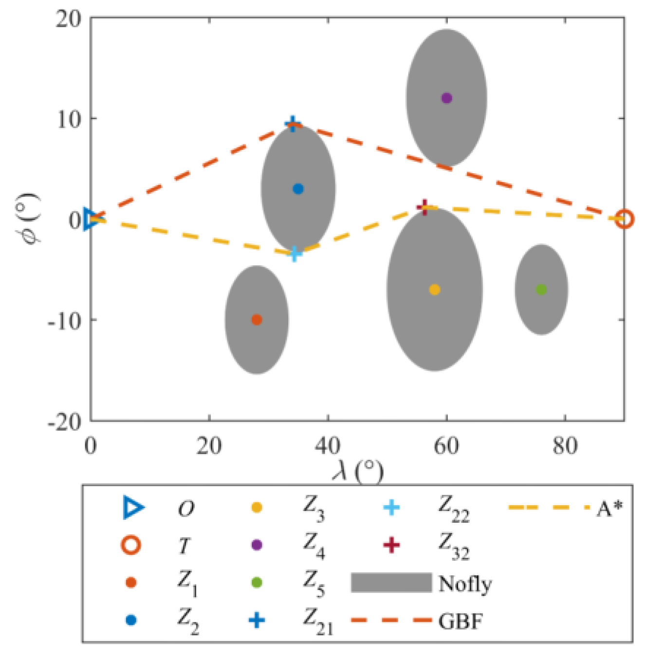
6.3. Avoidance Search Results Under Multiple No-Fly Zones

To compare the effects of the A* waypoint search algorithm under the multiple no-fly zones, the greedy best-first (GBF) search algorithm in Ref. [37] is selected for comparative simulation. The two searched avoidance trajectories are displayed in Figure 7. The set of waypoints from $O\to$$Z_{22}\to$$Z_{32}\to$$T$ of the A* algorithm have the minimum value of the evaluation function with $J_{A*,\min }\left(O\right)=0.6449$. The search of the GBF algorithm is based on target, rather than full search. GBF prioritizes the expansion of waypoints close to the target, which means a small heuristic function value, so its search speed is faster. The set of waypoints from $O\to$$Z_{21}\to$$T$ of the GBF algorithm have the minimum value of the evaluation function with $J_{GBF,\min }\left(O\right)=0.6876$. Therefore, by comparing the minimum evaluation function of the two methods, the avoidance path of the A* algorithm reduced the value of the evaluation function by 6.2%, demonstrating its optimality for solving avoidance path searches in multi-no-fly zone conditions and achieving an optimal energy consumption for the HMV.

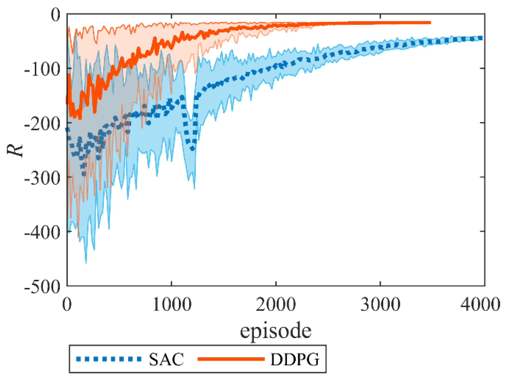
6.4. Training Results of RL

Following 3600 episodes of RL training for coordinated reentry guidance, the cumulative rewards trajectory is visualized in Figure 8, where the deterministic policy gradient-based DDPG algorithm is benchmarked against soft Actor–Critic (SAC) algorithm [38] to evaluate their control performance. As depicted in Figure 3, the DDPG algorithm demonstrates superior convergence velocity and stability metrics compared to its SAC counterpart. Quantitatively, the reward function of the DDPG framework progressively converges to a stabilized maximum value of approximately −16, whereas the SAC algorithm plateaus at a significantly lower reward magnitude of −43. This substantial performance disparity indicates that the morphing policy network instantiated by the DDPG algorithm achieves an optimal mission-specific parameterization.

The DDPG training process, comprising 3600 episodes, is executed offline on a workstation equipped with an NVIDIA RTX 4070 GPU, requiring approximately 10 h for completion. Only the finalized policy network architecture featuring four hidden layers with 100 neurons per layer is deployed onboard. Performance benchmarks conducted on an Intel Core i7 CPU using Torch 2.1 demonstrate a model memory footprint of 122.2 kB and a mean inference time of 0.1 ms. This time is significantly below the 50 ms guidance cycle requirement, confirming real-time operational feasibility for deployment on modern embedded systems possessing comparable computational capabilities.

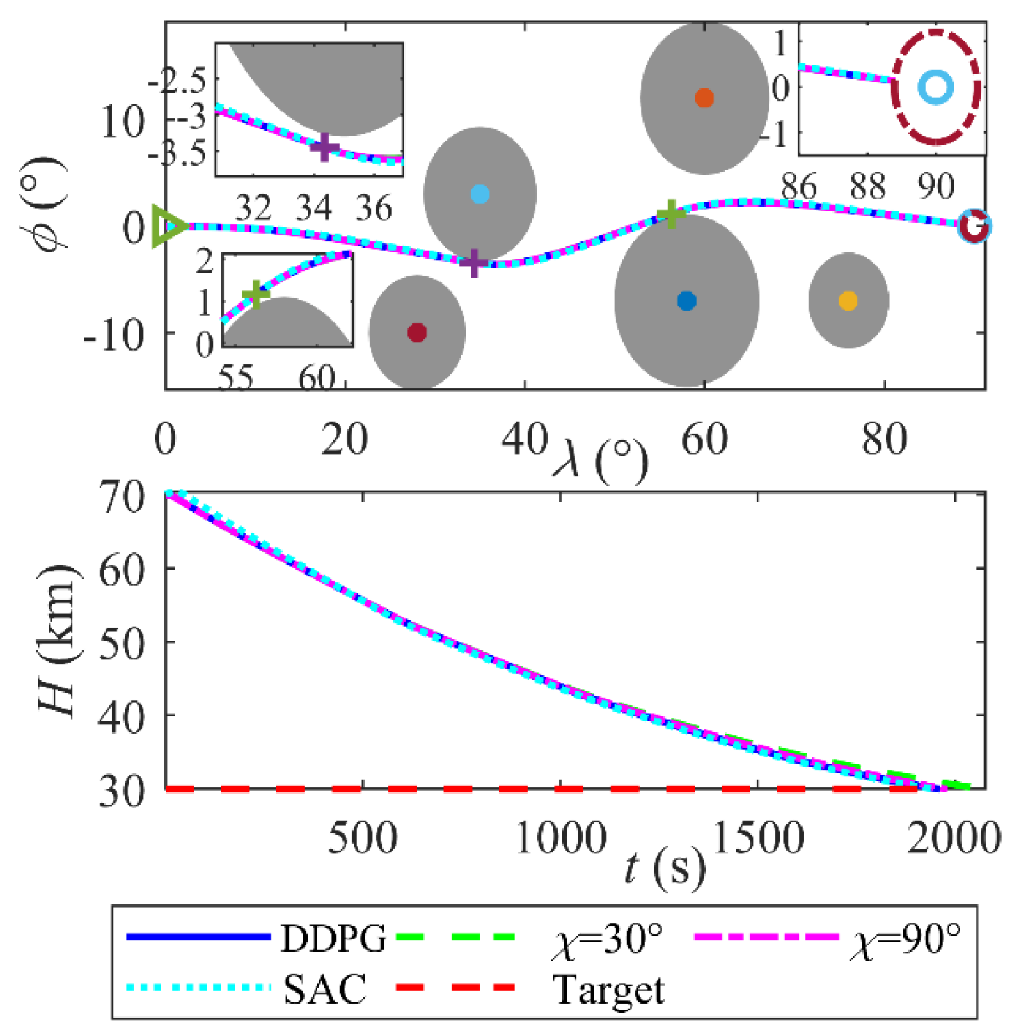
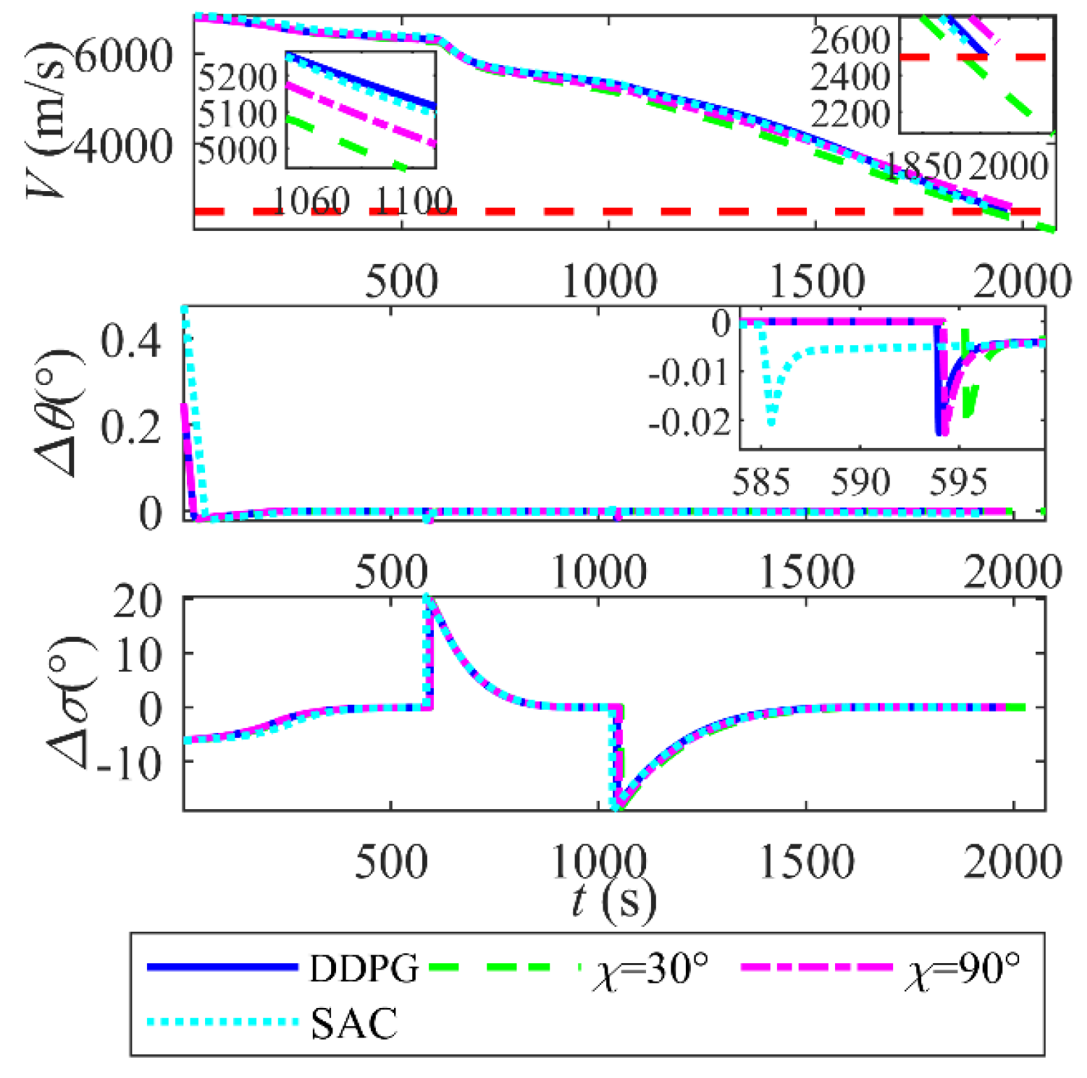
6.5. Effectiveness of the Intelligent Coordinated Guidance Method

In order to verify the effectiveness of the coordinated guidance method, the no-fly zone waypoint search algorithm, the QEGC guidance law, and the morphing policy network are substituted into the reentry flight simulation of the HMV. To compare the effect of the morphing policy of the DDPG algorithm, three control groups, including two with a fixed morphing of $\chi ={30}^{°}$ and $\chi ={90}^{°}$ and the morphing policy of the SAC algorithm [38] are set. The simulation results are shown in Figure 9, Figure 10 and Figure 11. The average tracking errors of terminal range error $\Delta S_f$, terminal velocity error $\Delta V_f$, terminal velocity of avoidance flight $V_{Z_{32}}$, and the average tracking error of flightpath angle ${\Sigma }_{\Delta \theta }$ of the four morphing policies are shown in Table 1.

Table 1. Comparisons of reentry flight variables.

Variables	DDPG	χ = 30°	χ = 90°	SAC
$\Delta S_f\left(\mathrm{km}\right)$	−0.09	0.01	0.24	0.39
$V_{Z_{32}}\left(\mathrm{m}/\mathrm{s}\right)$	5275.0	5074.14	5181.86	5260.2
$\Delta V_f\left(\mathrm{m}/\mathrm{s}\right)$	−0.01	−419.39	80.61	87.23
${\Sigma }_{\Delta \theta }\left(°\cdot \mathrm{s}\right)$	$1.87\times {10}^{-3}$	$1.96\times {10}^{-3}$	$1.89\times {10}^{-3}$	$1.97\times {10}^{-3}$

Table 1. Comparisons of reentry flight variables.

Variables	DDPG	χ = 30°	χ = 90°	SAC
$\Delta S_f\left(\mathrm{km}\right)$	−0.09	0.01	0.24	0.39
$V_{Z_{32}}\left(\mathrm{m}/\mathrm{s}\right)$	5275.0	5074.14	5181.86	5260.2
$\Delta V_f\left(\mathrm{m}/\mathrm{s}\right)$	−0.01	−419.39	80.61	87.23
${\Sigma }_{\Delta \theta }\left(°\cdot \mathrm{s}\right)$	$1.87\times {10}^{-3}$	$1.96\times {10}^{-3}$	$1.89\times {10}^{-3}$	$1.97\times {10}^{-3}$

where ${\Sigma }_{\Delta \theta }$ is defined as follows:

$${\Sigma }_{\Delta \theta }={\displaystyle \underset{0}{\overset{T}{\int }}\Delta \theta \left(t\right)\mathrm{d}t}$$

(68)

where $T$ is the total flight time. Figure 9 and Figure 10 show that the proposed coordinated guidance method can guide the HMV from the starting position to the TAEM interface without crossing the no-fly zones, and the terminal position error is kept below 0.1km. The terminal altitude error requirement is satisfied, since the simulation is cut off by the altitude. As shown in Figure 11 and Table 1, at the last avoidance waypoint $Z_{32}$, the velocity of the RL morphing policy is the largest, 5275.0m/s, indicating that the reward function setting of DDPG can effectively reduce the velocity loss during the avoidance flight. Compared to SAC, DDPG’s deterministic policy network achieves a 0.09 km terminal position error, 75% lower than SAC’s 0.39km error, and a 0.01 m/s terminal velocity error, outperforming fixed morphing’s −87.23m/s error. This benefits from the DDPG algorithm’s greater learning ability. Comparing the terminal velocities of the three groups, the terminal velocity error of the DDPG morphing policy is only 0.01 m/s, while that of the three control groups are −419.39 m/s, 80.61 m/s, and 87.23 m/s, respectively. So, the reward function setting of DDPG can effectively reduce the terminal velocity error. Under the positive flightpath angle tracking error, the tracking error with $\chi ={30}^{°}$ is smaller due to the larger lift of the small sweep angle. By contrast, for negative flightpath angle tracking error, the error under $\chi ={90}^{°}$ is smaller because of the smaller lift of the large sweep angle. Therefore, it can be seen from Table 1 that the average tracking error of the flightpath angle under the DDPG morphing policy is the smallest, $1.87\times {10}^{-3}$, because of the adjustable sweep angle according to a different flight state. The errors of the heading angle are gradually eliminated during the flight time between waypoints and satisfy the terminal to heading angle constraint.

According to Figure 12, the angles of attack and bank angles under the three morphing policies are within the constraints of the control inputs and maintain the QEGC gliding flight in the longitudinal and lateral directions. Compared with the two fixed morphing groups, the sweep angle of the DDPG morphing policy is relatively more complex. The sweep angle will be kept at 30° to increase the lift to achieve upward tracking under the large positive tracking error. Otherwise, the sweep angle will be kept at 90° to decrease the lift to achieve downward tracking. During the avoidance flight with no-fly zones, the sweep angle is kept near the optimal sweep angle corresponding to the maximum lift-to-drag ratio, so as to increase the lift-to-drag ratio, reduce the velocity loss during the avoidance flight, and retain more energy for the subsequent mission. Figure 13 shows that the constraints of heat rate density, dynamic pressure, and overload are all kept below the corresponding constraints to keep a safe reentry flight.

By comprehensive timing measurements, pre-trained A* planning completes in under 0.1 ms. The DDPG policy achieves a 0.1 ms inference on Intel processors. The integrated planning–guidance cycle maintains a 1.60 ms average execution per step—just 3.2% of the 50 ms operational window. These metrics validate real-time feasibility for avionics deployment through significant computational margin retention.

6.6. Generalization of Intelligent Coordinated Guidance Method

The above simulation results are trained for a single mission, and in order to check the results of the generalization of the intelligent coordinated guidance method for different missions, other flight targets different from the training mission are given for simulations. Three different groups of target positions are set as T1 (85°, 16°), T2 (80°, −13°), and T3 (88°, −6°). Figure 14 shows that the proposed coordinated guidance method presents a good generalization performance and guides the HMV from the starting point to the TAEM interface of different targets without crossing the multiple no-fly zones. The terminal position and no-fly zone constraints are satisfied. The terminal position errors of T1, T2, and T3 are −0.21 km, −0.24 km, and −0.09 km, respectively. As shown in Figure 15, in three different flight targets, the terminal velocity errors are 5.90 m/s, 1.74 m/s, and 3.67 m/s, which are within the allowed range. This adherence to the allowed range indicates that the DDPG morphing policy can effectively constrain the terminal velocity. The tracking of the velocity bank angle, as well as the heading angle, satisfy the heading angle constraint. From Figure 16, it can be seen that the changes to the angle of attack and bank angle under the three different flight targets are within the input constraints. The DDPG morphing policy can cope well, making an autonomous adjustment to the sweep angle according to the flight missions. Figure 17 demonstrates that the path constraints are satisfied under the three different flight targets.

6.7. Robustness of the Intelligent Coordinated Guidance Method

To test the robust performance of the designed intelligent morphing coordinated guidance method, Monte Carlo experiments are performed under given random deviations of initial state, atmospheric density, and aerodynamic coefficients. In order to improve the adaptability of the deterministic DDPG algorithm to the nondeterministic environment, a correction term $\Delta \chi =-k_V\left(V-V_r\right),k_V=0.04$ can be added to the sweep angle output from the policy network, where $V_r$ is the reference velocity in the nominal environment. Assuming that the deviations of the initial state, the atmospheric density, and the aerodynamic coefficient have the standard normal distribution, the $3\sigma$ deviations are given as follows: ${\Delta }_{H_0}=100 \mathrm{m}$, ${\Delta }_{{\lambda }_0}={0.5}^{°}$, ${\Delta }_{{\varphi }_0}={0.5}^{°}$, ${\Delta }_{V_0}=100 \mathrm{m}/\mathrm{s}$, ${\Delta }_{{\theta }_0}={0.5}^{°}$, ${\Delta }_{{\sigma }_0}={0.5}^{°}$, ${\Delta }_{\rho }=20\%$, ${\Delta }_{C_L}=10\%$, and ${\Delta }_{C_D}=10\%$. Gaussian noise with $V_{\sigma }=10 \mathrm{m}/\mathrm{s}$ and $H_{\sigma }=10 \mathrm{m}$ were added to the velocity and altitude measurements, respectively. To mimic real-world actuator dynamics, a first-order delay ranging from 0.1 to 0.3s was applied to the sweep angle commands.

The obtained trajectories and velocities of the 1000 Monte Carlo experiments are shown in Figure 18. The results show that the designed intelligent coordinated guidance method can accomplish the reentry of the mission with no-fly zones under the deviations of the initial state, atmospheric density, and aerodynamic coefficient. The statistics of terminal position and velocity of the Monte Carlo experiments are presented in Figure 19. The mean value of terminal range error is 0.263 km, and the standard deviation is 0.184 km, while the mean value of terminal velocity error is −12.7 m/s, and the standard deviation is 42.93 m/s. Therefore, the errors of terminal range and velocity are within the allowed range, providing clear visual evidence of the method’s resilience to sensor noise, actuator delays, and parameter uncertainties in the reentry flight. Figure 20 shows the sweep angle variation curve with time delay. Figure 21 shows that the path constraints and flight safety are satisfied in Monte Carlo experiments.

The control framework’s inherent robustness is underpinned by two key mechanisms: DDPG’s adaptive learning capability enabling the policy network to learn and generalize across diverse uncertain dynamics during offline training for effective real-world performance, and a tanh-based sliding mode control layer in the guidance loop ensuring the finite-time convergence of tracking errors even under bounded disturbances for added stability and resilience.

7. Conclusions

This paper introduces an intelligent morphing coordinated reentry guidance method for hypersonic morphing vehicles (HMVs) under multiple no-fly zone constraints. The key contributions and findings are summarized as follows:

• A hybrid framework integrating A* trajectory planning, DRL-based morphing control, and QEGC guidance law is proposed. The A* algorithm systematically generates energy-optimal avoidance trajectories by resolving waypoints within complex no-fly zones, outperforming the greedy best-first search method (GBF) with a 6.2% reduction in evaluation function value.
• RLs provide an online implementation of policy network solutions for autonomous optimal morphing decision. The DDPG algorithm trains a morphing policy network to adaptively adjust the sweep angle in real time. The DDPG policy requires 122.2 kB memory and a 0.1ms inference time on an Intel Core i7, meeting the 50ms guidance period time.
• The coordination guidance law of DDPG and QEGC ensures precise longitudinal and lateral tracking via continuous switching sliding mode control. Compared to fixed morphing policies and a SAC-based control, the proposed approach reduces the terminal position error to 0.09 km and terminal velocity error to 0.01m/s. The reward-driven DDPG policy optimizes velocity retention during avoidance maneuvers, achieving a terminal velocity of 5275.0 m/s and improving by at least 93m/s compared to the fixed sweep. Moreover, it maintains the minimum tracking error.
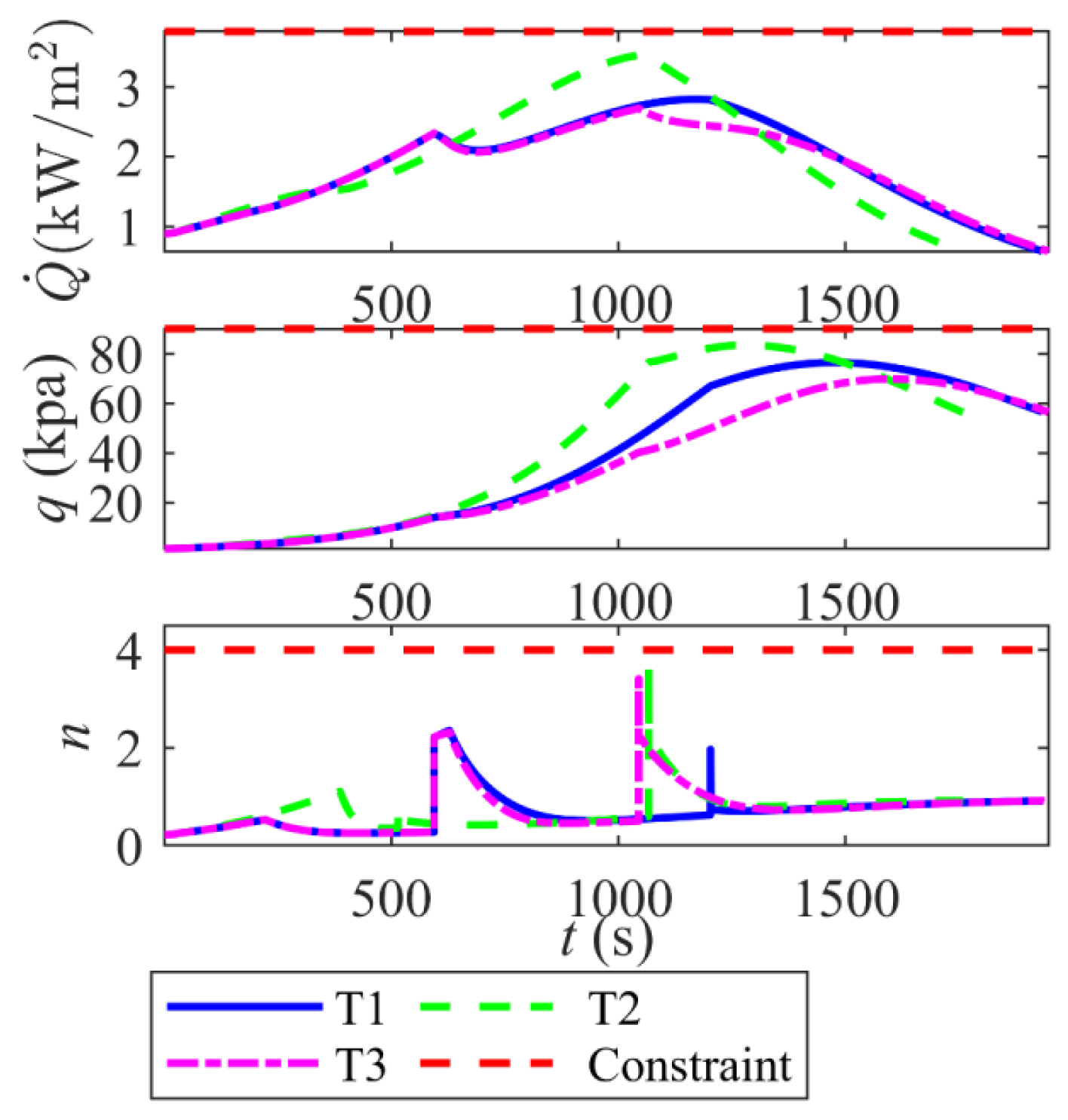
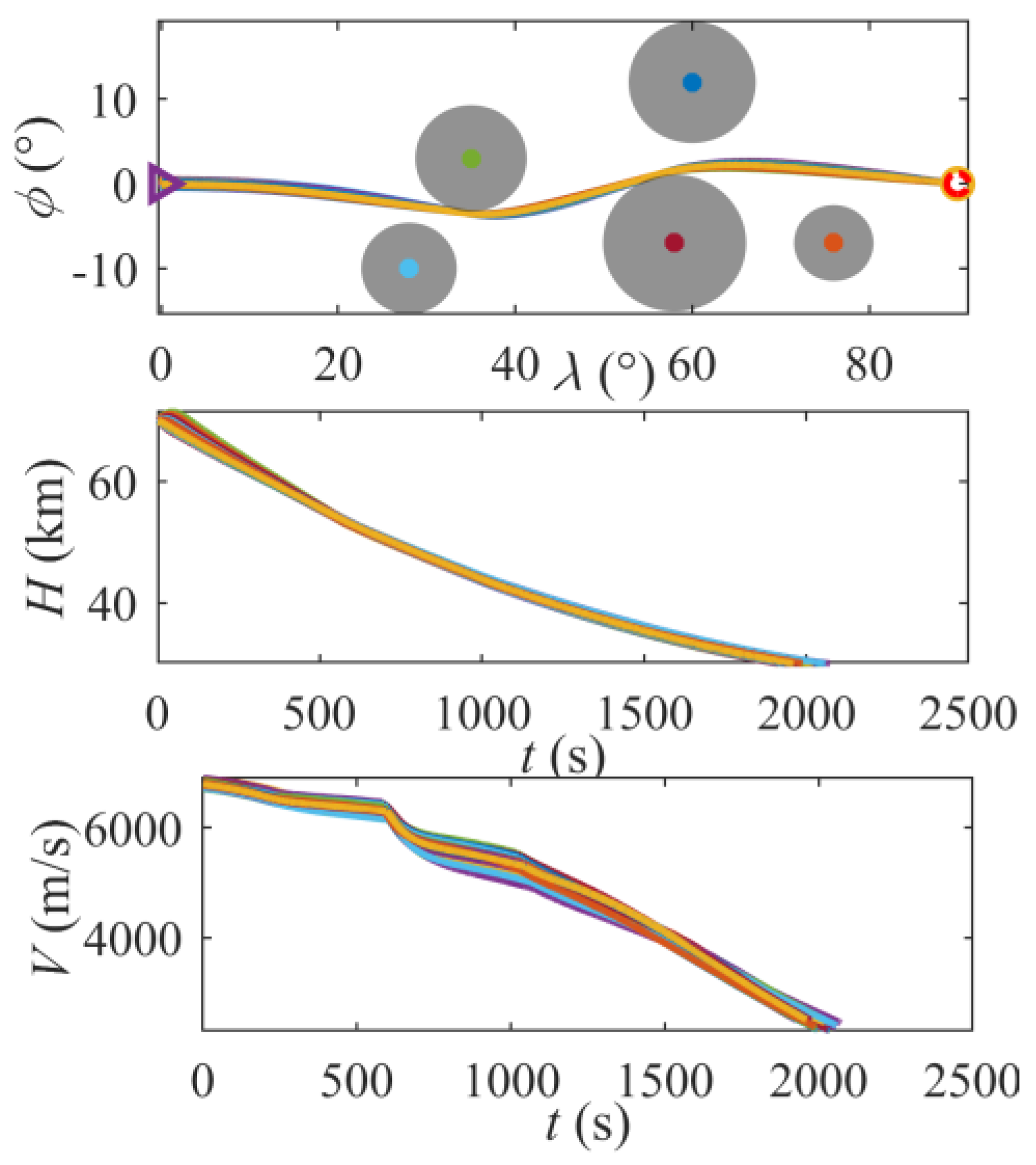
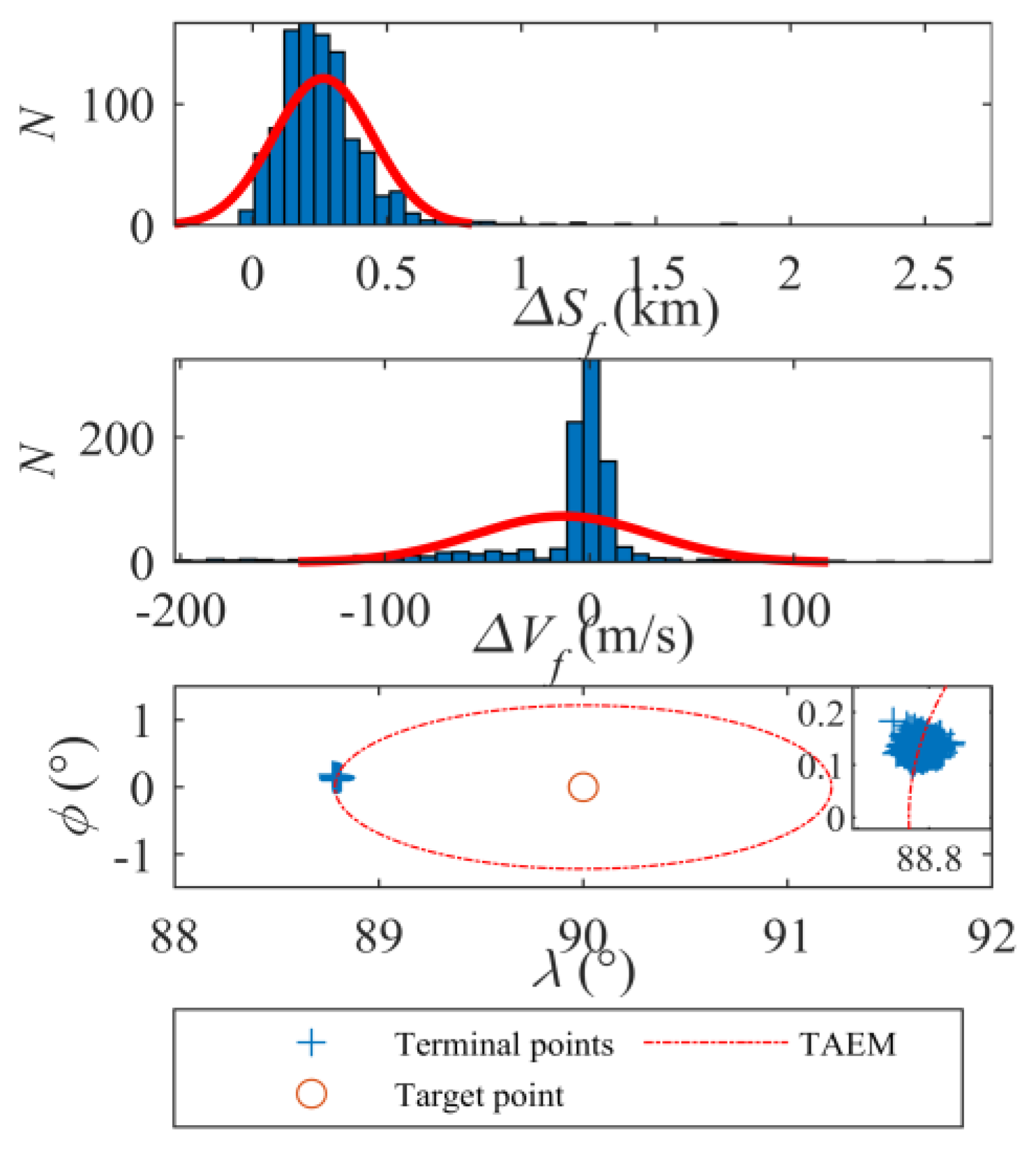
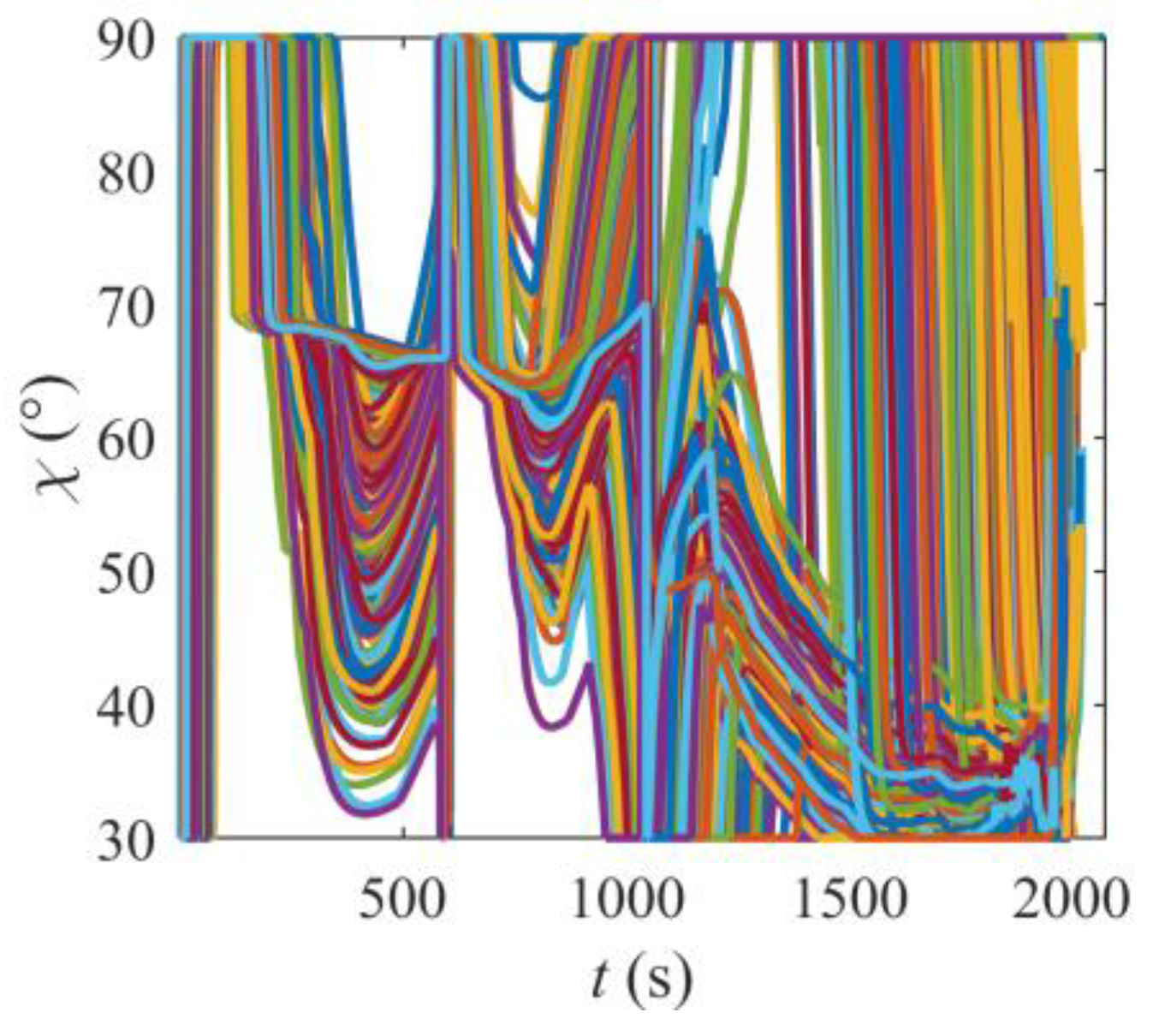
• The framework demonstrates robust generalization and adaptability. Monte Carlo simulations validate its robustness, with terminal range errors confined to 0.263 km (mean) ± 0.184 km (std) and velocity errors to −12.7 m/s (mean) ± 42.93 m/s (std). Additionally, tests across three distinct target missions (T1–T3) show consistent terminal position errors below 0.24 km and velocity errors under 5.90 m/s, confirming the method’s capability to generalize beyond training scenarios.
• This study bridges trajectory planning, adaptive morphing, and robust guidance for HMVs. By synergizing A*’s global optimization with DRL’s real-time adaptability, the method ensures safe reentry under stringent path constraints. Future work will focus on implementing model pruning and computational acceleration to further optimize the policy network for deployment on flight-grade embedded processors.

References

1. Jin, Z.; Yu, Z.; Meng, F.; Zhang, W.; Cui, J.; He, X.; Lei, Y.; Musa, O. Parametric Design Method and Lift/Drag Characteristics Analysis for a Wide-Range, Wing-Morphing Glide Vehicle. Aerospace 2024, 11, 257. [Google Scholar] [CrossRef]
2. Dai, P.; Yan, B.; Huang, W.; Zhen, Y.; Wang, M.; Liu, S. Design and aerodynamic performance analysis of a variable-sweep-wing morphing waverider. Aerosp. Sci. Technol. 2020, 98, 105703. [Google Scholar] [CrossRef]
3. Cheng, L.; Li, Y.; Yuan, J.; Ai, J.; Dong, Y. L1 Adaptive Control Based on Dynamic Inversion for Morphing Aircraft. Aerospace 2023, 10, 786. [Google Scholar] [CrossRef]
4. Li, D.; Zhao, S.; Da Ronch, A.; Xiang, J.; Drofelnik, J.; Li, Y.; Zhang, L.; Wu, Y.; Kintscher, M.; Monner, H.P.; et al. A review of modelling and analysis of morphing wings. Prog. Aeronaut. Sci. 2018, 100, 46–62. [Google Scholar] [CrossRef]
5. Chu, L.; Li, Q.; Gu, F.; Du, X.; He, Y.; Deng, Y. Design, modeling, and control of morphing aircraft: A review. Chin. J. Aeronaut. 2022, 35, 220–246. [Google Scholar] [CrossRef]
6. Cai, G.; Shang, Y.; Xiao, Y.; Wu, T.; Liu, H. Predefined-Time Sliding Mode Control with Neural Network Observer for Hypersonic Morphing Vehicles. IEEE Trans. Aerosp. Electron. Syst. 2025, 1–17. [Google Scholar] [CrossRef]
7. Bao, C.; Wang, P.; Tang, G. Integrated guidance and control for hypersonic morphing missile based on variable span auxiliary control. Int. J. Aerosp. Eng. 2019, 2019, 6413410. [Google Scholar] [CrossRef]
8. Zhou, X.; He, R.-Z.; Zhang, H.-B.; Tang, G.-J.; Bao, W.-M. Sequential convex programming method using adaptive mesh refinement for entry trajectory planning problem. Aerosp. Sci. Technol. 2021, 109, 106374. [Google Scholar] [CrossRef]
9. Dai, P.; Feng, D.; Feng, W.; Cui, J.; Zhang, L. Entry trajectory optimization for hypersonic vehicles based on convex programming and neural network. Aerosp. Sci. Technol. 2023, 137, 108259. [Google Scholar] [CrossRef]
10. Lu, P.; Brunner, C.W.; Stachowiak, S.J.; Mendeck, G.F.; Tigges, M.A.; Cerimele, C.J. Verification of a fully numerical entry guidance algorithm. J. Guid. Control Dyn. 2017, 40, 230–247. [Google Scholar] [CrossRef]
11. Zhu, J.; Liu, L.; Tang, G.; Bao, W. Robust adaptive gliding guidance for hypersonic vehicles. Proc. Inst. Mech. Eng. Part G 2018, 232, 1272–1282. [Google Scholar] [CrossRef]
12. Zhu, J.; Zhang, S. Adaptive Optimal Gliding Guidance Independent of QEGC. Aerosp. Sci. Technol. 2017, 71, 373–381. [Google Scholar] [CrossRef]
13. Yao, D.; Xia, Q. Finite-Time Convergence Guidance Law for Hypersonic Morphing Vehicle. Aerospace 2024, 11, 680. [Google Scholar] [CrossRef]
14. Huang, S.; Jiang, J.; Li, O. Adaptive Neural Network-Based Sliding Mode Backstepping Control for Near-Space Morphing Vehicle. Aerospace 2023, 10, 891. [Google Scholar] [CrossRef]
15. Fazeliasl, S.B.; Moosapour, S.S.; Mobayen, S. Free-Will Arbitrary Time Cooperative Guidance for Simultaneous Target Interception with Impact Angle Constraint Based on Leader-Follower Strategy. IEEE Trans. Aerosp. Electron. Syst. 2025, 1–15. [Google Scholar] [CrossRef]
16. Xie, Y.; Liu, L.; Liu, J.; Tang, G.; Zheng, W. Rapid generation of entry trajectories with waypoint and no-fly zone constraints. Acta Astronaut. 2012, 77, 167–181. [Google Scholar] [CrossRef]
17. He, R.; Liu, L.; Tang, G.; Bao, W. Rapid generation of entry trajectory with multiple no-fly zone constraints. Adv. Space Res. 2017, 60, 1430–1442. [Google Scholar] [CrossRef]
18. Hu, Y.; Gao, C.; Li, J.; Jing, W.; Chen, W. A novel adaptive lateral reentry guidance algorithm with complex distributed no-fly zones constraints. Chin. J. Aeronaut. 2022, 35, 128–143. [Google Scholar] [CrossRef]
19. Zhang, D.; Liu, L.; Wang, Y. On-line reentry guidance algorithm with both path and no-fly zone constraints. Acta Astronaut. 2015, 117, 243–253. [Google Scholar] [CrossRef]
20. Wang, S.; Ma, D.; Yang, M.; Zhang, L.; Li, G. Flight strategy optimization for high-altitude long-endurance solar-powered aircraft based on Gauss pseudo-spectral method. Chin. J. Aeronaut. 2019, 32, 2286–2298. [Google Scholar] [CrossRef]
21. Zhang, R.; Xie, Z.; Wei, C.; Cui, N. An enlarged polygon method without binary variables for obstacle avoidance trajectory optimization. Chin. J. Aeronaut. 2023, 36, 284–297. [Google Scholar] [CrossRef]
22. Zhang, Y.; Zhang, R.; Li, H. Graph-based path decision modeling for hypersonic vehicles with no-fly zone constraints. Aerosp. Sci. Technol. 2021, 116, 106857. [Google Scholar] [CrossRef]
23. Radmanesh, R.; Kumar, M.; French, D.; Casbeer, D. Towards a PDE-based large-scale decentralized solution for path planning of UAVs in shared airspace. Aerosp. Sci. Technol. 2020, 105, 105965. [Google Scholar] [CrossRef]
24. AlShawi, I.S.; Yan, L.; Pan, W.; Luo, B. Lifetime enhancement in wireless sensor networks using fuzzy approach and A-star algorithm. In Proceedings of the IET Conference on Wireless Sensor Systems (WSS 2012), London, UK, 18–19 June 2012; IET: London, UK, 2012; pp. 1–6. [Google Scholar] [CrossRef]
25. Zhang, Z.; Zhao, Z. A multiple mobile robots path planning algorithm based on A-star and Dijkstra algorithm. Int. J. Smart Home 2014, 8, 75–86. [Google Scholar] [CrossRef]
26. Dai, P.; Feng, D.; Zhao, J.; Cui, J.; Wang, C. Asymmetric integral barrier Lyapunov function-based dynamic surface control of a state-constrained morphing waverider with anti-saturation compensator. Aerosp. Sci. Technol. 2022, 131, 107975. [Google Scholar] [CrossRef]
27. Dai, P.; Yan, B.; Han, T.; Liu, S. Barrier Lyapunov Function Based Model Predictive Control of a morphing waverider with input saturation and full-state constraints. IEEE Trans. Aerosp. Electron. Syst. 2023, 59, 3071–3081. [Google Scholar] [CrossRef]
28. Chen, X.; Li, C.; Gong, C.; Gu, L.; Ronch, A.D. A study of morphing aircraft on morphing rules along trajectory. Chin. J. Aeronaut. 2021, 34, 232–243. [Google Scholar] [CrossRef]
29. Fasel, U.; Tiso, P.; Keidel, D.; Ermanni, P. Concurrent Design and Flight Mission Optimization of Morphing Airborne Wind Energy Wings. AIAA J. 2021, 59, 1254–1268. [Google Scholar] [CrossRef]
30. Bao, C.; Wang, P.; Tang, G. Integrated method of guidance, control and morphing for hypersonic morphing vehicle in glide phase. Chin. J. Aeronaut. 2021, 34, 535–553. [Google Scholar] [CrossRef]
31. Xu, W.; Li, Y.; Pei, B.; Yu, Z. Coordinated intelligent control of the flight control system and shape change of variable sweep morphing aircraft based on dueling-DQN. Aerosp. Sci. Technol. 2022, 130, 107898. [Google Scholar] [CrossRef]
32. Xu, D.; Hui, Z.; Liu, Y.; Chen, G. Morphing control of a new bionic morphing UAV with deep reinforcement learning. Aerosp. Sci. Technol. 2019, 92, 232–243. [Google Scholar] [CrossRef]
33. Hou, L.; Liu, H.; Yang, T.; An, S.; Wang, R. An Intelligent Autonomous Morphing Decision Approach for Hypersonic Boost-Glide Vehicles Based on DNNs. Aerospace 2023, 10, 1008. [Google Scholar] [CrossRef]
34. Tenenbaum, J.B.; Kemp, C.; Griffiths, T.L.; Goodman, N.D. How to grow a mind: Statistics, structure, and abstraction. Science 2011, 331, 1279–1285. [Google Scholar] [CrossRef] [PubMed]
35. Bao, C.Y.; Zhou, X.; Wang, P.; He, R.Z.; Tang, G.J. A deep reinforcement learning-based approach to onboard trajectory generation for hypersonic vehicles. Aeronaut. J. 2023, 127, 1638–1658. [Google Scholar] [CrossRef]
36. Silver, D.; Lever, G.; Heess, N.; Degris, T.; Wierstra, D.; Riedmiller, M. Deterministic Policy Gradient Algorithms. In Proceedings of the 31st International Conference on International Conference on Machine Learning-Volume 32, Bejing, China, 21–26 June 2014; JMLR.org: Beijing, China, 2014; pp. I-387–I-395. [Google Scholar]
37. Heusner, M.; Keller, T.; Helmert, M. Best-Case and Worst-Case Behavior of Greedy Best-First Search. In Proceedings of the 27th International Joint Conference on Artificial Intelligence (IJCAI 2018), Stockholm, Sweden, 13–19 July 2018; International Joint Conferences on Artificial Intelligence Organization: Stockholm, Sweden, 2018; pp. 1463–1470. [Google Scholar] [CrossRef]
38. Wu, Y.; Sun, G.; Xia, X.; Xing, M.; Bao, Z. An Improved SAC Algorithm Based on the Range-Keystone Transform for Doppler Rate Estimation. IEEE Geosci. Remote Sens. Lett. 2013, 10, 741–745. [Google Scholar] [CrossRef]
Figure 1. Intelligent coordinated reentry guidance scheme.
Aerospace 12 00591 g001
Figure 2. Morphing mode of HMV.
Aerospace 12 00591 g002
Figure 3. Effect of morphing on the lift-to-drag ratio at different Mach (a) Ma = 6; (b) Ma = 13; (c) Ma = 20.
Aerospace 12 00591 g003
Figure 4. Schematic diagram of the HMV’s trajectory and the no-fly zones.
Aerospace 12 00591 g004
Figure 5. Multiple no-fly zones graph modeling.
Aerospace 12 00591 g005
Figure 6. Schematic diagram of the DDPG algorithm.
Aerospace 12 00591 g006
Figure 7. Multiple no-fly zone avoidance trajectory.
Aerospace 12 00591 g007
Figure 8. Variation in cumulative reward with episodes.
Aerospace 12 00591 g008
Figure 9. Three-dimensional reentry trajectory of gliding section.
Aerospace 12 00591 g009
Figure 10. Variations in latitude, longitude, and altitude.
Aerospace 12 00591 g010
Figure 11. Variations in velocity, tracking errors of flightpath angle, and heading angle.
Aerospace 12 00591 g011
Figure 12. Variations curve of control input.
Aerospace 12 00591 g012
Figure 13. Variations in the path constraints.
Aerospace 12 00591 g013
Figure 14. Variations in latitude, longitude, and altitude.
Aerospace 12 00591 g014
Figure 15. Variations in velocity, tracking errors of flightpath angle, and heading angle.
Aerospace 12 00591 g015
Figure 16. Variations curve of control input.
Aerospace 12 00591 g016
Figure 17. Variations of the path constraints.
Aerospace 12 00591 g017
Figure 18. Variations in latitude, longitude, and altitude of Monte Carlo experiments.
Aerospace 12 00591 g018
Figure 19. Statistics of terminal range error, velocity error, and landing point position.
Aerospace 12 00591 g019
Figure 20. Variations curve of sweep angle with delay of Monte Carlo experiments.
Aerospace 12 00591 g020
Figure 21. Variations of the path constraints of Monte Carlo experiments.
Aerospace 12 00591 g021
Disclaimer/Publisher’s Note: The statements, opinions and data contained in all publications are solely those of the individual author(s) and contributor(s) and not of MDPI and/or the editor(s). MDPI and/or the editor(s) disclaim responsibility for any injury to people or property resulting from any ideas, methods, instructions or products referred to in the content.