1. Introduction
Since the early 1980s, the National Aeronautics and Space Administration (NASA) has carried out a tracking project on the operational status of over 7000 aircraft in the subsequent 20 years. Reports from this project show that engine failures accounted for 36% of aircraft entering non-airworthy conditions [
1], with the failure rate of gas path components exceeding 90%. The operational costs for restoring their performance constituted over 60% of the fleet’s total maintenance costs [
2,
3].
It can be seen that aircraft engines, as strongly nonlinear systems, continuously operate under complex aerothermodynamic conditions featuring high temperatures, high pressure, high speeds, and strong vibrations. Their component structures and performance inevitably degrade, leading to engine mechanical failures and even system breakdown failures [
4,
5]. The rotational speeds of engine shafts, along with pressures and total temperatures at various flow field sections, serve as state parameters for engine gas path components. These are important reference indicators for assessing engine health status.
Research routes based on information fusion across multiple domains and disciplines are receiving increasing attention from researchers. Gas path fault diagnosis technologies for aircraft engines can be primarily classified into the following three categories.
(1) Model-based gas path fault diagnosis methods typically integrate the working characteristics of the engine flow field with its structure. They solve the nonlinear co-working equations between components through optimization algorithms to obtain various characteristic parameters during system steady-state operation. This approach can intuitively reveal the internal operational mechanism of the engine while facilitating parameter configuration. Dufour G and Thollet W [
6] introduced a body force modeling simulation method based on classical CFD simulation, thoroughly revealing the flow field mechanism of the DGEN380 engine. Zhu et al. [
7] presented a nonlinear state-space model grounded in gas turbine prior knowledge. This model is better suited for multi-input systems like aircraft engines, and its polynomial form ensures stability during global computation. A corrected equilibrium manifold expansion (CEME) model utilizing gas turbine prior knowledge was developed. The equilibrium manifold dimensionality is increased by incorporating similarity equations, replacing high-dimensional polynomial fitting. The dynamic similarity criterion from similarity theory ensures the global stability of the CEME model. Volponi et al. [
8] performed matrix solving on the established system model. They also investigated the application of streaming full flight data encompassing both transient and steady-state operation. Properly processed, this data stream enables faster anomaly detection, reliable fault persistency verification, and timely fault identification. Zhou et al. [
9] achieved fault diagnosis using estimated parameters from an identified model and performance indicator residuals under healthy conditions. Initially, to estimate missing measurements, forward and backward algorithms were formulated based on corresponding component models according to failure hypotheses. Subsequently, a novel fault diagnosis logic was devised, and the conventional nonlinear filter was enhanced by incorporating a measurement estimation module and a health parameter correction module. This module employs reconstructed measurements to finalize health parameters estimation. The simulation outcomes demonstrate the method’s capability to effectively restore the intended measurement. Diagnosis methods based on linear models generally also incorporate parameter estimation and state estimation techniques. Chang [
10] explored health parameter estimation in an aeroengine using an unknown input observer-based approach, executed via a second-order sliding mode observer. Differing from conventional state estimator-based methods, this scheme utilizes a “reconstruction signal” to estimate health parameters modeled as artificial inputs. It is not only applicable to long-term health degradation but also responds more rapidly to abrupt faults. Considering inevitable uncertainties in engine dynamics and modeling, a weighting matrix is formulated to minimize their estimation impact through linear matrix inequalities (LMI). Chang [
11] examines an integrated online sensor fault diagnostic scheme for a commercial aircraft engine using a sliding mode observer (SMO). This approach designs one SMO for engine health performance tracking and another for sensor fault reconstruction. The results from the first SMO are analyzed to update the baseline model of the second post-flight. This concept is practical and feasible as the update process eliminates the need for algorithm reconfiguration or redesign, thereby avoiding ground-based intervention and enabling economical, efficient implementation. Lu [
12] proposes a nonlinear hybrid model-based method for performance estimation and abnormal detection. An adaptive extended Kalman particle filter estimator is developed for real-time estimation of engine health parameters indicating gas turbine performance degradation. These estimators are stored in buffer memory for periodic baseline model renewal. The renewed model detects engine anomalies throughout its lifecycle, with detection thresholds adapting to modeling errors over the engine’s operational life. Brotherton et al. [
13] integrated Kalman filter theory into an onboard adaptive model, achieving estimation of engine component performance parameters. This method overcomes the low diagnostic accuracy inherent in traditional approaches due to complex fault characteristics. The identified fault parameters can further facilitate fault isolation.
The fundamental principle of fault diagnosis based on nonlinear engine models involves examining the statistical distribution relationship between the model’s theoretical output and the actual measured output. With the continuous advancement of nonlinear filtering theory, increasing research focuses on fault diagnosis using nonlinear filters. Borguet et al. [
14] employed an extended Kalman estimator for gas path fault diagnosis with an established model, incorporating error correction to enhance diagnostic system performance. Yan [
15] proposed that a fault detection and isolation system utilizing the UKF method removes the need to create different hypothetical models for hierarchical multiple-model-based FDI. Furthermore, a fault identification module based on the weighted sum of squared residuals from a filter bank is introduced to confirm the actual fault. The corresponding fault magnitude is subsequently estimated to adaptively update the fault diagnosis system parameters based on the confirmed fault. The proposed scheme achieves diagnostic accuracies of 97.3% and 93%. Simon D [
16] compared LKF, EKF, and UKF filters for accuracy and computational load in aircraft engine health estimation. While the unscented Kalman filter avoids Jacobian calculations, its computational demand is high due to requiring multiple simulations per time step. The EKF, recalculating Jacobians approximately every three flights, is identified as the optimal choice for aircraft engine health estimation. Wang et al. [
17] established a single rotor-bearing system dynamics model based on actual engine rotor fault morphologies, creating irregular fault models for bearing inner and outer rings. A vibration response simulation and analysis validated the accuracy of these fault models [
18]. An adaptive square root cubature Kalman filter (ASRCKF) was developed for turbofan engine gas path component fault diagnosis. The algorithm calculates the mean and covariance of the engine nonlinear function via a third-order cubature rule-based numerical integration method, replacing the nonlinear model to circumvent parameter selection issues encountered in the nonlinear unscented Kalman filter [
19]. The Sigma Point Kalman Filter was applied for gas turbine health parameter estimation and fault diagnosis. A discrete nonlinear mechanism model of the gas turbine was formulated, followed by the design of an improved Sigma Point Kalman Filter using simplex sampling. The results indicate that the diagnosis system possesses accurate detection, stable tracking performance, and good adaptability to fault modes and gas turbine operational conditions. Fang [
20] investigated a multi-model-based hybrid Kalman filter fault diagnosis method. This method employs a nonlinear airborne model to accommodate engine degradation levels and utilizes probability density functions for hypothesis testing, effectively resolving threshold selection and evaluation challenges. Jin [
21] examined the extended Kalman filtering approach for aircraft engine gas path analysis considering control loop parameter uncertainty. A novel method for gas path performance anomaly detection was presented, relying on combinations of recovered and actual measurements. Independently tuned adaptive onboard engine models with state buffers were designed for the real engine. Sensor and actuator fault isolation logic was developed using hybrid matrices [
22]. Addressing the Kalman filter’s susceptibility to misjudging gas path health parameters in commercial aircraft engines due to unevenly distributed and limited on-board sensors relative to health parameters, a neural network corrected Kalman filter algorithm was introduced. Algorithm individuals were corrected by a Back Propagation Neural Network. Their weights were calculated based on a particle filter during each sampling period to estimate mean and covariance. The Kalman Filter was then used to update the individuals.
(2) Data-based fault diagnosis methods can circumvent the need to establish complex aerothermodynamic models but impose high demands on data volume and distribution. Primary technical approaches include models based on neural networks, expert systems, fuzzy theory, as well as methods grounded in theories like deep belief networks and hidden Markov models. Additional approaches based on techniques such as spectrum analysis, wavelet transforms, autoregressive moving averages, and correlation functions constitute signal processing technologies that directly extract changing feature information of relevant variables to detect faults.
This approach disregards the internal operational mechanisms of the system. Instead, it constructs fault diagnosis models by employing data processing and statistical methods to solve the mapping relationship between inputs and outputs. Ossai and Chinedu [
23] derived component degradation rates from engine condition data and used this to analyze the system’s mean time to failure. Ellefsen et al. [
24] investigated the remaining useful life of aircraft engines using a semi-supervised learning approach, partially overcoming the traditional method’s heavy reliance on large labeled training datasets. Shang Lin [
25] developed an aircraft engine fault diagnosis model based on an artificial neural network, validating its effectiveness through case studies. However, the inherent drawbacks of shallow neural networks include their low generalization capability and poor performance, especially with insufficient datasets, when handling complex classification problems.
(3) Deep learning can better learn data features from limited samples. It employs deep nonlinear network structures to approximate complex functions in classification tasks, thereby enhancing classification capability and generalization performance. Its mainstream architectures include deep belief networks, deep Boltzmann machines, autoencoders, convolutional neural networks (CNNs), and RNNs [
26]. Wang et al. [
27] implemented fault diagnosis for aeroengine inter-shaft bearings using CNN. Yuan et al. [
28] proposed a gas path fault diagnosis model based on CNN, leveraging its strengths to accurately identify the health status of the engine gas path. Ma et al. [
29], addressing the inapplicability of traditional data feature extraction methods to aeroengine oil monitoring data, proposed a single-channel network model based on multi-scale CNNs, Long Short-Term Memory neural networks, and BP networks. This model serially extracts two-dimensional features of data in spatial and temporal dimensions using a multi-scale learning concept. Its overall performance surpasses traditional feature extraction methods like CNN and LSTM, meeting the real-time and accuracy requirements of aeroengine oil monitoring.
(4) The application of artificial neural networks in engine gas path diagnosis mainly involves diagnostic models established based on BP networks, convolutional neural networks, autoencoders, self-organizing feature mapping networks, and their improved algorithms. Extreme Learning Machines (ELMs) require shorter learning times while offering strong generalization capability, making them widely used in engine fault diagnosis. To address the insufficient sparsity of the original Kernel Extreme Learning Machine (KELM), LU F et al. [
30] introduced the concept of sub-learning machines and fused classification outputs based on DS evidence theory, significantly improving fault recognition speed. Lu et al. proposed an improved ELM featuring an iterative sparse selection scheme [
31]. During validation for aeroengine gas path fault diagnosis, this method reduced the computational load of classification tasks to some extent.
Support Vector Machine-based methods essentially perform global optimization for convex quadratic programming tasks by introducing structural risk minimization. Verified, this method rarely suffers from overfitting or underfitting and holds unique advantages for classification tasks with small training samples. However, its application to engine gas path fault diagnosis faces challenges such as kernel function selection and regularization parameter determination.
(5) Fusion-based methods integrate the advantages of the two aforementioned research approaches. Typically, they model based on historical monitoring data while considering component degradation and failure mechanisms, simultaneously establishing accurate physical models of the corresponding systems. The data model is embedded into the physical model, yielding a fusion model capable of accurately simulating the performance degradation process or fault states. The tunable parameter feature endows this method with strong scalability. For instance, by assessing multi-state degradation principles and introducing model selection structures, Moghaddass and Zuo [
32] developed an online diagnosis and prognostics system. Zaccaria et al. [
33] proposed an adaptive performance model incorporating a probabilistic Bayesian network tailored for fleet engine fault detection characteristics, and conducted simulation validation. It was shown that the condition-based hierarchical model achieved superior accuracy, and the benefit was more significant for data with higher overlap between states.
In recent years, the trend of interdisciplinary research has increasingly highlighted the importance of information fusion methods. The fundamental idea of information fusion is to generalize the data to be processed within the same conceptual space and perform fusion and output based on mathematical methods [
34]. Among existing domestic and international research, gas path fault diagnosis methods based on theories such as DS evidence fusion, Bayesian fusion, and fuzzy fusion are numerous. Lu [
35] diagnosed gas path faults using DS evidence theory fusion by adjusting weights, combined with an improved support vector regression machine. By fusing model and data feature information, engine gas path fault diagnosis was achieved.
Guo et al. [
36] presented a mechanical fault time series prediction method combining multiple sparse autoencoder error fusion with Long Short-Term Memory. By fusing errors from multiple sparse autoencoder layers, multi-feature time series were extracted and fused into a prediction error trend curve. The irregular trends in the squared prediction error trend curve were then predicted using LSTM. The results demonstrated the effectiveness of this method in mechanical fault time series prediction.
Fu et al. [
37] conducted a bench test for electrostatic monitoring of an aero-turbojet engine. Utilizing electrostatic signal data, they mitigated the limitation of single information sources in traditional aeroengine gas path performance diagnosis. An engine performance evaluation method fusing electrostatic signals and gas path parameters was proposed and solved using a logistic regression model. The experimental results indicated that this fusion evaluation method outperformed traditional performance assessment techniques and enabled early warning of gas path faults.
(6) For existing research on Kalman filtering, Donald L. Simon [
38] developed a robust sensor fault detection and isolation (FDI) system for aircraft engines using a novel bank of (m + 1) Kalman filters. Its key innovation lies in the dedicated architecture: one filter detects component/actuator faults, while m filters each target a specific sensor fault. This design significantly enhances robustness against misclassification of non-sensor anomalies, improving diagnostic reliability. The system’s effectiveness is validated through nonlinear engine simulations under multiple power settings and various fault scenarios. Donald L. Simon [
39] proposed a constrained Kalman filter via analytic truncation of the state estimate’s probability density function at physical boundaries. This method improves estimation accuracy for turbofan engine health monitoring over unconstrained filters and projection-based alternatives, validated via engine simulations. D. Simon [
40] extended Kalman filtering to incorporate statistical state constraints (linear equality constraints on state expectations); derived a parameterized family of constrained filters via a weighting matrix, ensuring that the estimates satisfy these constraints while maintaining optimality properties; and analyzed the mathematical foundations of this constrained estimation approach. Dan Simon [
41] proposed an adaptive Kalman filter that switches between constrained and unconstrained estimation based on residual confidence levels. When confidence in the unconstrained (optimal) estimate is high, constraints are disabled; otherwise, heuristic physical constraints are applied. This balances theoretical optimality with robustness, validated via turbofan engine health estimation simulations. S. Borguet [
42] compared two adaptive Kalman filter-based tools for gas turbine performance monitoring, specifically targeting improved detection of abrupt faults. Standard KFs excel at tracking gradual deterioration but struggle with rapid faults due to smooth transition model assumptions. Both proposed tools integrate secondary residual monitoring systems (one using covariance matching and the other a Generalized Likelihood Ratio Test—GLR) to enhance fault detection speed and localization for abrupt changes. S. Borguet [
43] proposed a combined PCA-Kalman filter approach for online aircraft engine diagnostics. This original coupling leverages PCA’s dimensionality reduction and the KF’s estimation strength, enhancing diagnostic capability beyond either method alone. The benefit of the combined tool was demonstrated via simulated fault cases in a commercial turbofan.
Sébastien Borguet [
44] developed an adaptive Kalman filter for aircraft engine performance monitoring. It uses covariance matching to automatically relax constraints on slowly varying health parameters upon detecting abrupt faults, enabling simultaneous tracking of gradual deterioration and sudden failures.
The main problems in these fault diagnosis studies and the gaps this study aims to address are concentrated in the following:
(1) The frequent requirement to build large neural network models places significant pressure on the storage capacity of onboard systems. Simultaneously, high-precision neural network models have slow processing speeds, failing to meet the real-time requirements of onboard systems.
(2) For fault signatures with low occurrence rates, insufficient network training due to imbalanced samples leads to low fault recognition accuracy. While artificially injecting fault signatures at different operating points to expand the training set is an option, it cannot guarantee consistent impact of such faults on engine performance parameters across all operating points.
(3) For faults that have not occurred, the absence of fault samples renders machine learning-based methods incapable of identification.
2. Establishment of Component-Level Model
As a nonlinear system, an aeroengine exhibits a highly complex aerodynamic and thermodynamic operating process. Simulation technology enables the modeling of engine operations under complex working conditions and varying health states. A precise component-level model can accurately simulate engine startup, acceleration and deceleration, and operational states under different conditions. It also allows for the early implementation of modal simulations for the engine control system [
45,
46,
47]. Therefore, this section takes the JT9D aeroengine as the research object and establishes a nonlinear component-level model under cruise and small-range dynamic conditions. This model provides a full-envelope simulation platform capable of executable gas path parameter calculations, degradation simulations, and fault feature injections for subsequent research.
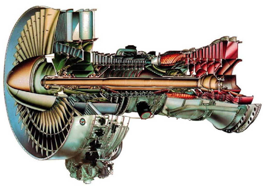
The JT9D engine, developed and manufactured by Pratt & Whitney, is the world’s first commercial engine designed for wide-body aircraft. Its structural and performance characteristics closely align with those of currently in-service engines used by airlines, making it a representative research subject. NASA has extracted and publicly released the aerodynamic and thermodynamic characteristics, constant coefficients, and steady-state data of JT9D core components from its modeling and analysis of thermodynamic systems project [
48]. The structural sectional view and the corresponding cross-section diagram is shown as
Figure 1 and
Figure 2:
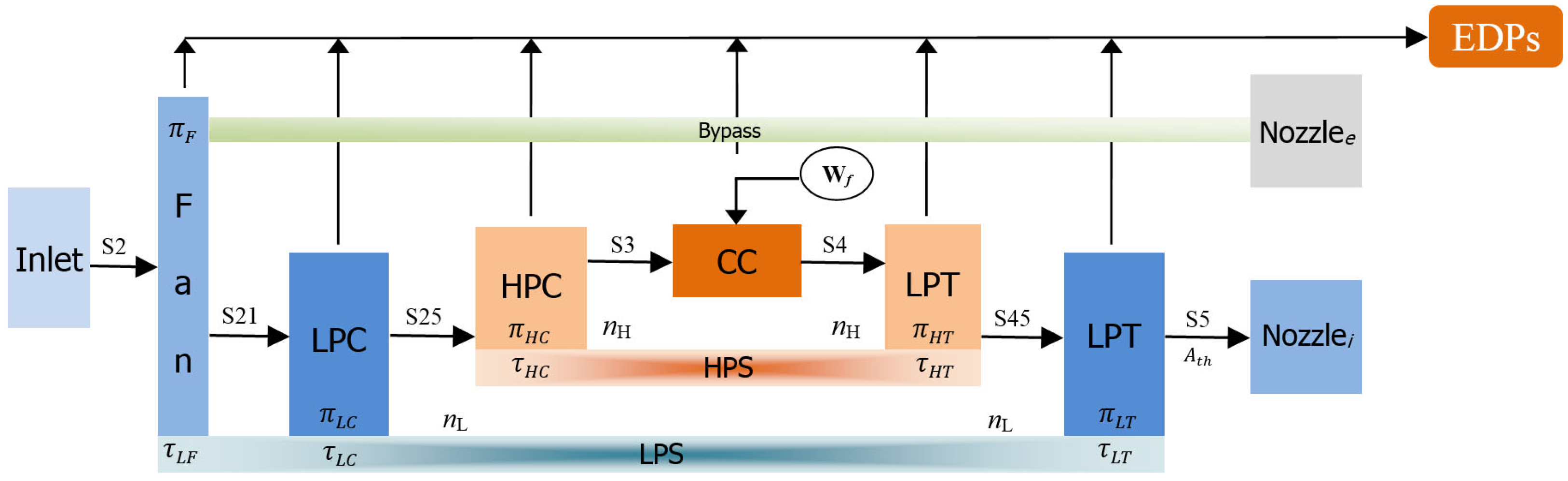
The JT9D engine primarily consists of 12 components [
49], as shown in
Figure 1: inlet, fan, low-pressure compressor (LPC), high-pressure compressor (HPC), combustion chamber (CC), low-pressure turbine (LPT), high-pressure turbine (HPT), core nozzle, bypass nozzle, bypass duct, low-pressure spool (LPS), and high-pressure spool (HPS).
The component-level engine model serves as a platform for characteristic parameter calculations and method validation of the fault diagnosis technology studied in this paper. Assuming that the engine operates in a stable laminar flow field, the effects of inertial and viscous forces on the airflow can be neglected. Additionally, the model assumes that fluid flow at the same time satisfies the principle of mass conservation [
50].
2.1. Aerothermodynamic Model
In the aerodynamic and thermodynamic calculations of the engine system, the system response cannot be uniquely determined based only on the input of each component. For a given shaft speed, the flow rate and pressure ratio of the compressor are not unique. Therefore, it is necessary to use the compressor characteristic map to solve for the compressor inlet flow rate. The calculated flow rate is then compared with the actual inflow to determine the flow error. During this process, component characteristic maps are employed to compute the efficiency, pressure ratio (PR), and corrected flow (WC), which are functions of the corrected speed Nc and running line. The running line in the characteristic map is utilized to adjust the operating point until the flow error reaches zero. It is dynamically computed by the iterative solver proposed in this study to satisfy the overall equilibrium conditions of the engine system, such as flow continuity and power matching. Since large multidimensional tables increase computational complexity and affect model-solving speed, the characteristic maps are decomposed into three separate tables, and interpolation is used to solve for WC, PR, and efficiency of the operating point.
This study leverages maps, constants, and steady-state data from NPSS-developed models for the creation of Simulink simulations. For components like the fan, compressors, and turbines, performance maps are directly utilized. For components that are not explicitly defined, like the inlet, the model is run at a steady-state point and then the inputs are perturbed to form a partial relation between the input and output flow variables. The rotor dynamics are added to the model using a representative rotational moment of inertia and the associated equations of motion, as the change in rotor speed is a function of torque differential between the turbine and compressor on a given rotor. Conservation of energy is ensured internally for each component, and mass is ensured by adding a solver that reconciles inter-component imbalances at every computation step.
The compressor and turbine modules use performance maps to compute efficiency, pressure ratio, and corrected flow. Because of the complication of creating a large multidimensional table in MATLAB R2024b, the compressor performance maps’ characteristics have been broken down into three different tables for interpolation, which solve for corrected flow, pressure ratio, and efficiency separately. Compressor efficiency, corrected flow, and pressure ratio are determined from the compressor map as functions of corrected shaft speed. Turbine efficiency and corrected flow are determined from the turbine map as functions of shaft speed and pressure ratio.
Modeling in this paper is based on nonlinear table lookups, which are accessed via the C-code and MATLAB script. These table lookups contain the thermodynamic properties of air and a hydrocarbon exhaust gas. Therefore, functions such as pt2sc described below are MATLAB table lookup functions to calculate enthalpy, entropy, and total temperature for specified components.
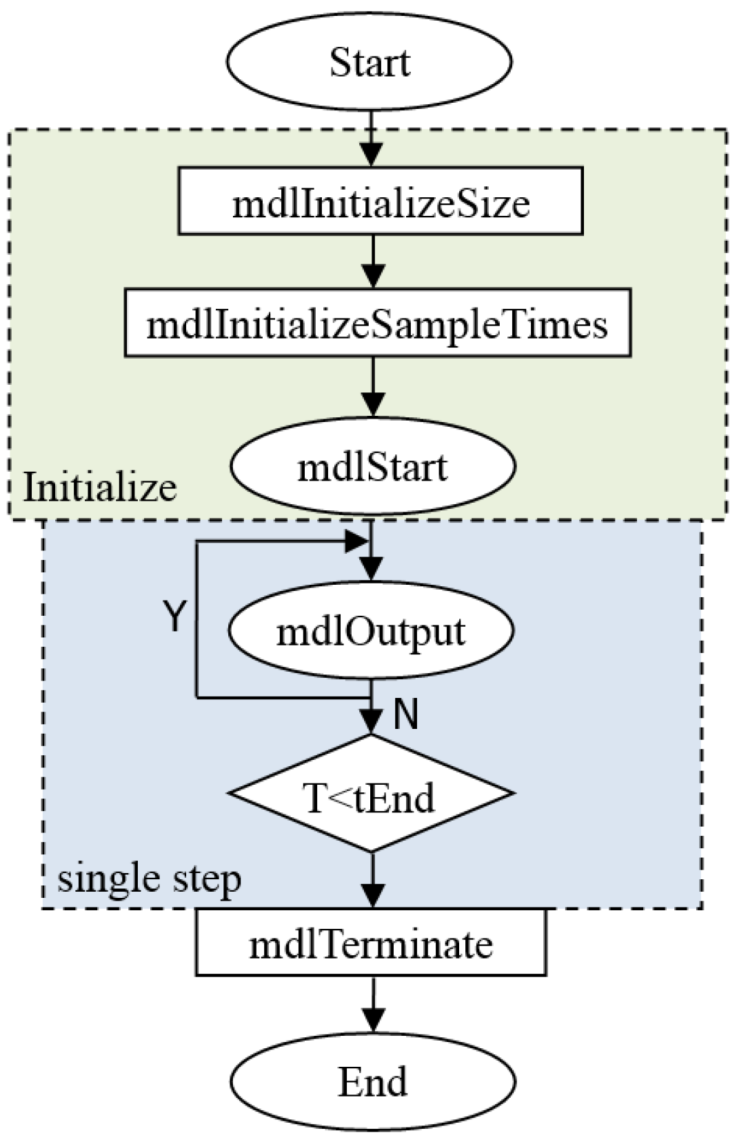
This paper uses an S-Function in Simulink to interpolate the characteristic data of each component [
51,
52], as shown in
Figure 3, thereby achieving numerical simulation of the parameters when the components are operating. After compiling the S-Function into a MEX file, each function is called. It mainly includes configuring initial states such as input and output, setting the S-Function sampling time, simulation initialization, computing function output, and terminating the function.
Based on the flow field structure of the JT9D gas path [
53], the thermodynamic processes of each component are modeled separately. Due to space limitations, this section focuses solely on the fan, compressor, and turbine. The specific process is as follows:
(1) Fan. The operating characteristics of the fan are obtained by interpolating its characteristic map, including efficiency, pressure ratio, rotational speed, and flow rate.
where
nc is the corrected speed of a low-pressure spool,
PRF is the pressure ratio of the fan.
The corrected mass flow and corrected rotational speed can be described based on the similarity theorem as follows:
where
represents the corrected total temperature,
T2 and
P2 are the fan inlet total temperature and pressure, and
represents the corrected total pressure (with reference values of
Pref = 101,325 Pa and
Tref = 288 K in this study).
Under ideal conditions, the enthalpy
h, entropy
S, and total temperature
T at the fan outlet are calculated using empirical formulas as follows:
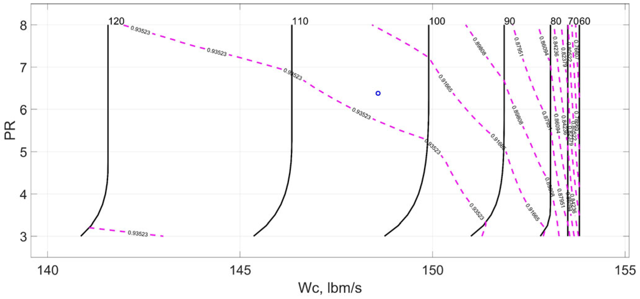
The actual outlet enthalpy h
21 and outlet total temperature
T21 can be further obtained through interpolation of the characteristic data in the characteristic map of
Figure 4, where pt2sc, sp2tc, t2hc, and h2tc are the computational functions for entropy, enthalpy, and total temperature. They are implemented by calling the table lookup program written in C language.
The power of the fan
GF is calculated based on the air mass flow W
21 and the enthalpy difference of the fan outlet:
(2) Compressor: Its function is to compress the upstream gas and perform work on it, significantly increasing the gas pressure. For a high-pressure compressor’s rated speed
nHd, inlet total temperature
T25, and the total temperature at design point
T25d, the equivalent speed
can be calculated based on the current high-pressure spool speed
nH as follows:
Next, interpolation is performed on the characteristic map as shown in
Figure 5 to calculate the equivalent flow rate
Wc3, pressure ratio PR
HC, and efficiency
. The total temperature
Tt3 and total pressure
Pt3 at the compressor outlet, as well as the gas flow
W3, can then be calculated using the following formulas:
where
Wcount is the intermediate stage air intake,
P25 is the compressor inlet total pressure,
P25d is the compressor inlet total pressure at the design point. FAR is the fuel-to-air flow ratio,
h3 is the compressor outlet enthalpy.
The calculation process for outlet entropy, inlet enthalpy value, and actual outlet enthalpy is similar to that of the fan component and will not be reiterated in this paper.
(3) Turbine. This paper takes the low-pressure turbine as an example to elaborate on its thermodynamic calculations. The outlet parameters of the low-pressure turbine are as follows:
where
Pt5 is the total pressure at the outlet section of the LPT,
W5 is the mass flow rate of the gas passing through the low-pressure turbine,
Pt45 is the total pressure at the inlet of LPT,
Pt45d is the total pressure at the inlet of LPT at the design point, and
Tt45 is the total temperature at the inlet of LPT.
The equivalent rotational speed
nLTcor is derived from the turbine air flow, the rotor design point speed, and the input rotational speed. Then, through interpolation function
F1 and
F2 using the characteristic map, the equivalent gas flow rate
Wc5 and efficiency
ηLT are obtained:
where
PRLPT is the pressure ratio of the LPT.
2.2. Steady-State Model
The steady-state model determines the stable operating performance of the engine under specified external conditions and throttle settings. For the components to work together at steady-state points, they must satisfy the characteristic requirements. For the JT9D engine, a twin-rotor, high-bypass-ratio, separate-exhaust turbofan satisfies the characteristics of continuous section flow, corresponding pressures, and balance of shaft power during stable operation. Therefore, the steady-state coupling equations are designed as follows:
- (1)
The inlet flow rate of the engine fan
W2 equals the sum of the inlet flow rate of the compressor
W25 and the flow rate of the bypass air
W18.
- (2)
The gas flow rate at the inlet of the HPT
WG
4 equals the sum of the gas flow rate at the compressor outlet
W3 and the supplied fuel flow rate
Wf.
- (3)
The gas flow rate at the outlet of HPT
WG
41 equals the gas flow rate at the inlet of LPT
WG
45 (the bleed/feed flow and cooling flow present in the actual flow field are neglected).
- (4)
The total flow rate at the nozzle outlet
W8 equals the sum of the engine bypass gas flow rate
W18 and the gas flow rate at the outlet of LPT
WG51:
- (5)
High-pressure spool power balance:
- (6)
Low-pressure spool power balance:
The steady-state parameters of the engine are obtained by solving the system of working equations. The error convergence variable is set as the Euclidean norm F(x) of the equation system to eliminate the difference in the magnitude of each variable as Equation (24). W2 is the fan inlet gas flow, W25 is the compressor inlet gas flow, W18 is the engine bypass gas flow, W3 is the compressor outlet gas flow, Wf is the fuel supply in the combustion chamber, WG4 is the HPT inlet gas flow, WG41 is the HPT outlet gas flow, WG45 is the LPT inlet gas flow, W8 is the nozzle exit flow, WG51 is the LPT outlet gas flow, GHPT is the work done by the HPT, GHPC is the work consumed by the compressor, GLPT is the work done by the LPT, GF is the work consumed by the fan, ηHS is the high-pressure rotor transmission efficiency, and ηLS is the low-pressure rotor transmission efficiency. GEX is the extra power extraction.
The existing algorithms are unable to directly obtain an accurate solution for the nonlinear steady-state working equation system as shown in Equation (24) [
54]. The Newton–Raphson (N-R) method is one of the effective approximation algorithms for solving nonlinear implicit equation systems. The N-R method operates iteratively, initially using test data of steady-state point flow parameters of the JT9D engine as a starting guess. The input is used in the established engine component-level model, and the aerothermodynamic parameters of each component are solved in the order of the airflow. The corresponding data is then input into the steady-state working equation system for preliminary calculation, resulting in a set of error values. These error values are then used as a reference to correct the input parameters, and the process is repeated until the absolute value of the error meets the expected precision.
Let the variable flow composed of the initial guess be denoted by
X, where
where
HPT_
PRin is the pressure ratio of the HPT,
LPT_
PRin is the pressure ratio of the LPT,
nLin is the low-pressure spool speed,
nHin is the high-pressure spool speed, and
W is the inlet gas flow.
The Newton–Raphson algorithm updates the initial guess as follows:
where
k = 0, 1, 2, …k;
is the solution of the parent input parameters;
is the better solution of the offspring; and
J is the Jacobian matrix.
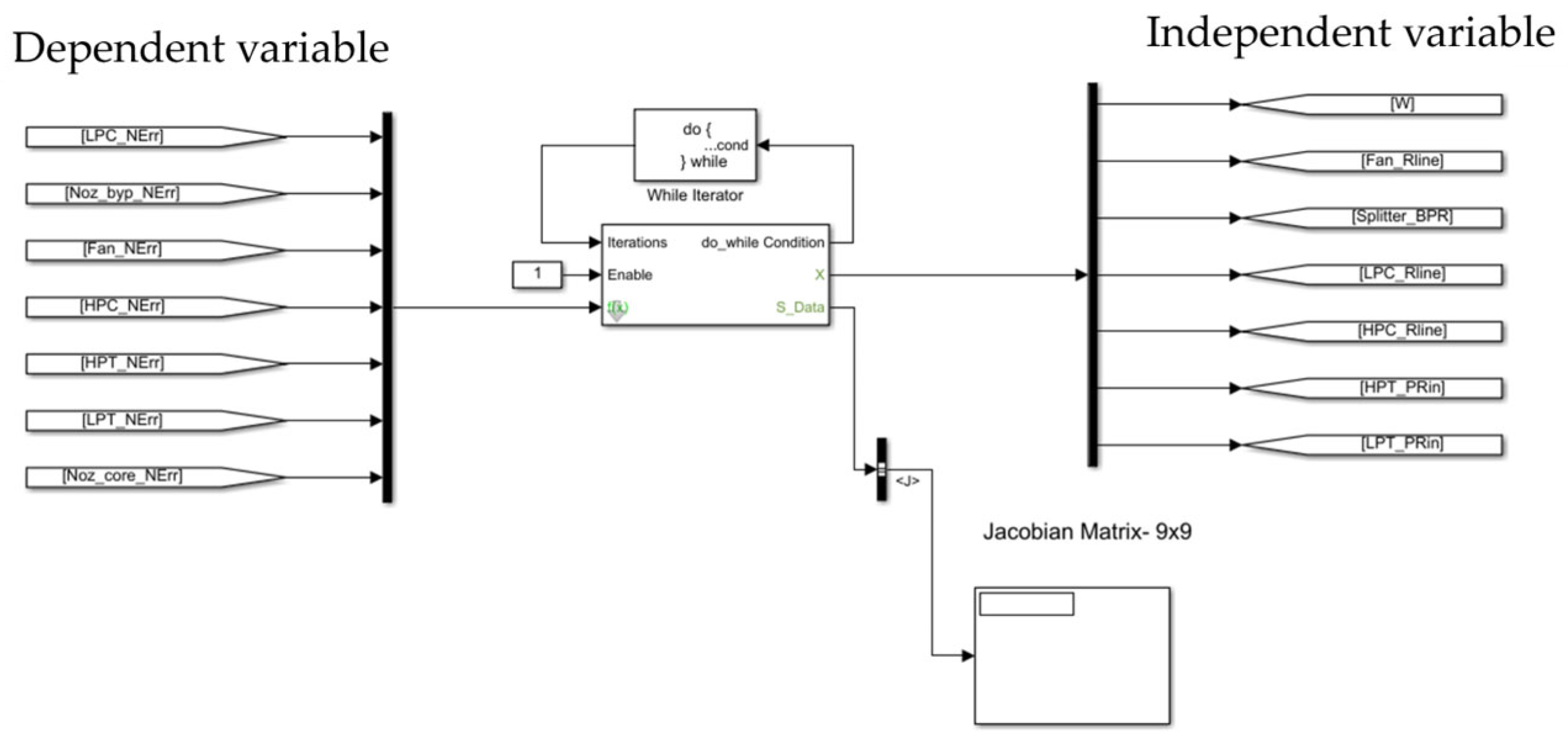
Jacobian matrix
J is the linear mapping between the inputs and outputs of the system. It is used to perturb each model input from the initial conditions
X to determine its effect on the model output
f(
x). The specific algorithm is as follows:
Next, a small perturbation is applied to the initial solution vector xj, such that . The partial derivatives are then computed using the forward difference method. The partial derivatives are used to construct the Jacobian matrix, and the corresponding j-th column of the Jacobian matrix is obtained. Firstly, the Jacobian solver computes the linear mapping of the model. Starting from the initial conditions, the Jacobian solver perturbs each input slightly and calculates the slope of each output as a function of each input. Once this step is completed for each input, the Jacobian matrix is constructed, inverted, and input into the N-R module. Secondly, the N-R solver uses the Jacobian matrix established in the first step to iteratively approach the solution.
Based on the N-R algorithm, the steady-state working equations of the engine component-level model established are solved under the design point operating conditions.
To verify the accuracy of the model established, a simulation is performed at takeoff conditions, with altitude, Mach number, and temperature set to 0 ft, 0, and 545.67 °R, respectively. A comparison between the parameters of the established model and the characteristic data defined by NPSS are presented in
Table 1.
The variation in the gas–thermal parameters at different component cross-sections during the iterative solution process is illustrated in
Figure 6. The horizontal axis indices correspond to different cross-sections: index 1 represents the fan inlet, index 2 represents the HPC inlet, index 3 represents the HPC outlet, index 4 represents the HPT inlet, index 5 represents the LPT inlet, and index 6 represents the LPT outlet. The algorithm for calculating the relative error is as follows:
where
m0 is the operating parameters of the engine under current operating conditions and
md is the operating parameters at the design point.
The results indicate that the maximum relative error between the steady-state values of the simulation model and the actual engine design point is 0.5757%, while the minimum is −0.0065%. This model meets the validation requirements for subsequent onboard fault diagnosis research.
2.3. Dynamic Simulation Model
The aeroengine inevitably undergoes acceleration or deceleration, and the working conditions with varying state variables and control variables correspond to dynamic processes [
55]. Compared to steady-state conditions, the working mechanisms of the engine’s flow field remain consistent. Therefore, the aerodynamic thermodynamic calculation process and the common working characteristic equations described in the previous section are also applicable to the dynamic model. The difference lies in the power balance deviation equations for the high- and low-pressure shafts in the dynamic model:
The power deviation equation for the high-pressure shaft during dynamic operation is as follows:
The power deviation equation for the low-pressure shaft during dynamic operation is as follows:
where
GHT is the HPT power,
GHC is the HPC power,
GLT is the LPT power,
GF is the fan power, and
GLC is the LPC power.
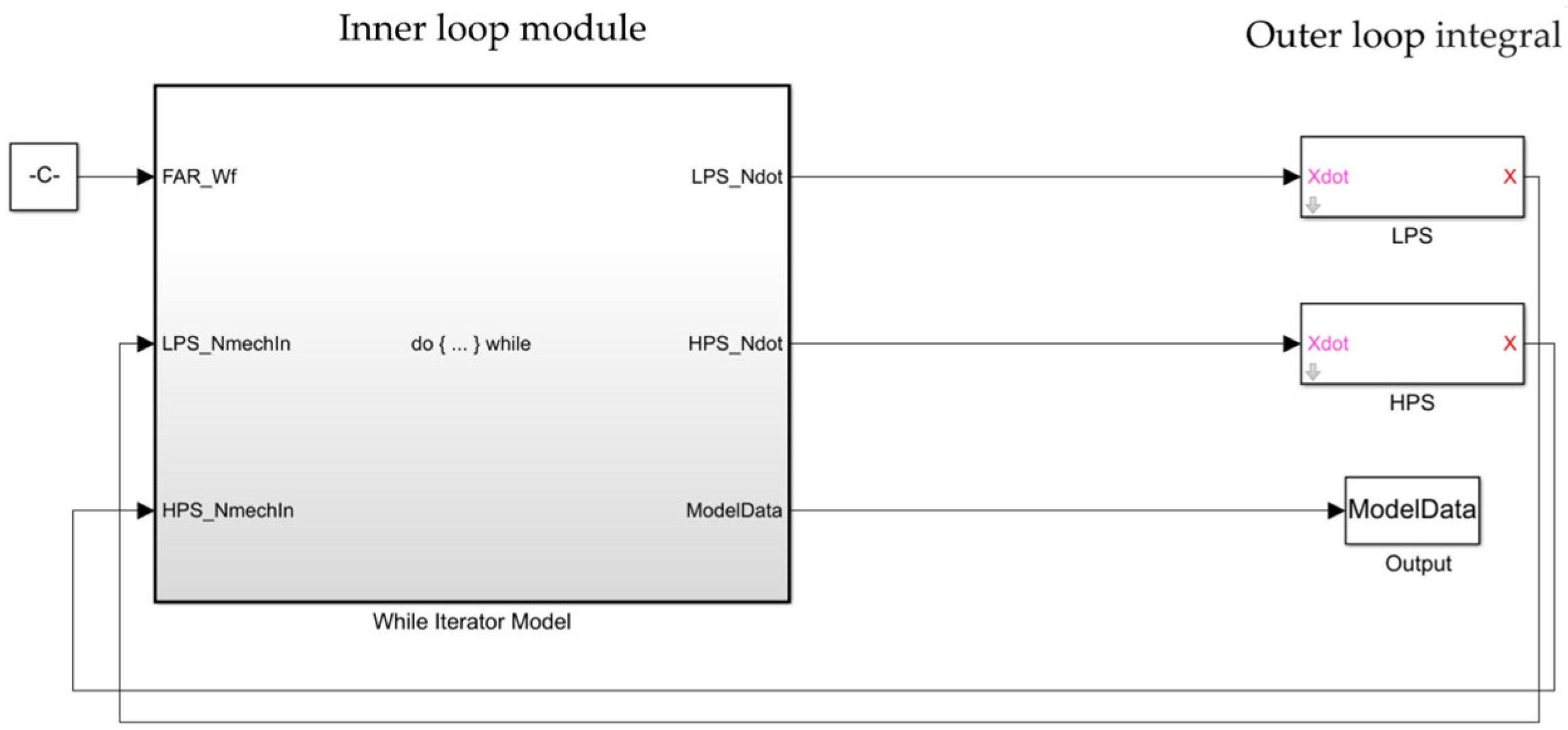
To simulate the dynamic process of the engine, the model introduces a dual loop iteration cycle. The inner loop is responsible for the convergence of the engine component-level model, while the outer loop iterates over time steps; the structure is shown in
Figure 7:
The inner loop model refers to the engine component-level model established in the previous section. The Do {…} While loop uses the While Iterator module in Simulink, combined with the Newton–Raphson algorithm, to iteratively solve the model. The outer loop module is an integration algorithm, with inputs being the high-pressure shaft acceleration
and the low-pressure shaft acceleration
(i.e., the time derivatives of the shaft speeds). These two parameters are integrated to output the actual high- and low-pressure shaft speeds. The established model at each level is shown in
Figure 8 and
Figure 9:
It can be observed that in the dynamic model, the input variable f(x) of the iterative solver corresponds to the output parameters of the component-level model, while the output variable x represents the input parameters of the component-level model. Compared to the Newton–Raphson solver used in the steady-state model, the solver in the dynamic model introduces additional inputs such as the number of iterations and outputs such as the loop termination condition. Iterative solving is performed at each time step until convergence is achieved in the dynamic model. If the system fails to converge, the simulation pauses at that time step to allow the system to reach convergence.
In summary, the operation of the dynamic model follows three steps: (1) The iterative solver introduces a perturbation to the engine model from the initial conditions and computes the Jacobian matrix based on the system response. (2) The N-R solver uses the inverse of the Jacobian matrix to iteratively solve the engine model. (3) If the convergence criteria are met, the algorithm terminates. If the input
f(
x) of the solver does not approach zero, the system fails to converge. The specific parameter used in the dynamic model solver are shown in
Table 2:
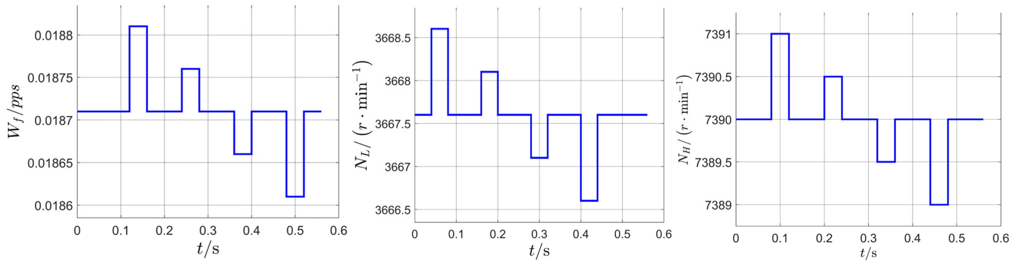
To validate the established dynamic model, a step change in fuel input is introduced. The fuel supply is evaluated using the fuel-to-air ratio as the indicator. The dynamic response of various gas path parameters in the model is shown in
Figure 10. The results indicate that the JT9D component-level model developed in this study successfully captures dynamic behavior. During acceleration and deceleration processes, the model outputs for high- and low-pressure shaft speeds align with rotor dynamics principles. This confirms that the model can serve as a reliable baseline for future research on model linearization and adaptive online fault diagnosis, providing robust airflow parameter support.
4. Onboard Adaptive Fault Diagnosis
The primary characteristics of gas path component faults include the following [
61,
62]: (1) Due to the intricate working mechanisms of gas flow fields, faults exhibit strong coupling, making it challenging to extract individual fault characteristics precisely. (2) Identical types of faults in the same type of component may present different characteristics under different operating conditions. Traditional approaches employ machine learning models [
63,
64,
65] to classify various engine operating data and extract fault characteristics and faulty components. However, these methods suffer from poor diagnostic capability when handling asymmetric data and have low real-time performance. Moreover, conventional fault diagnosis methods do not adequately address the issue of onboard model adaptability across the engine’s operating envelope [
66].
Considering that gas path faults lead to deviations in parameters such as rotational speed, temperature, and pressure from their nominal values, employing tracking algorithms such as Kalman filtering to estimate these parameters is a more reasonable and effective approach to realize fault diagnosis. Therefore, this section utilizes the augmented state-space model of the JT9D engine established in
Section 3, integrating an improved Kalman filter with actual engine operating states to track and estimate performance parameters that are unmeasurable across the entire flight envelope, to achieve a fault diagnosis.
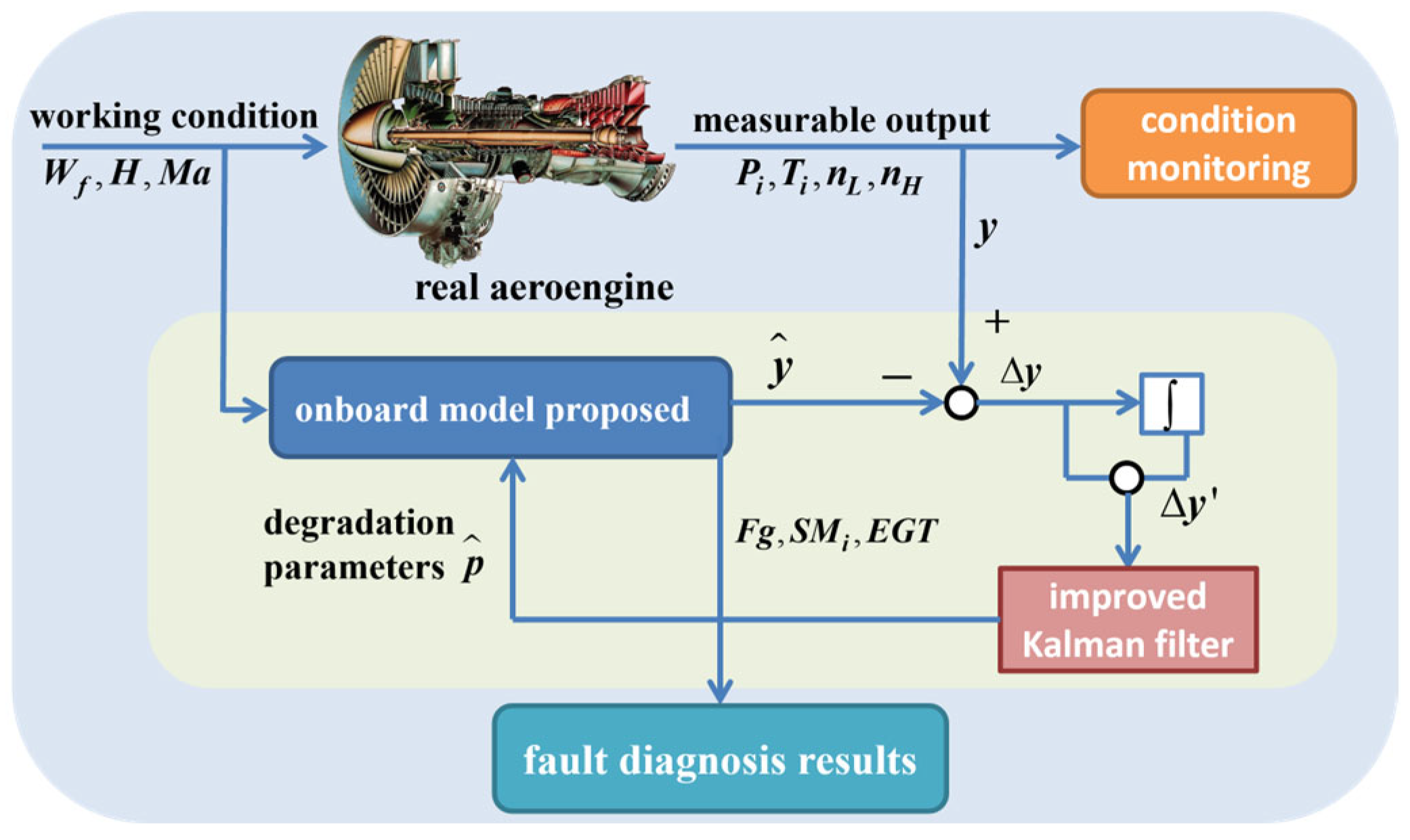
The core working principle is as follows: The onboard linear model receives the same operating states as the real engine, including fuel flow W
f, flight altitude
H, and Mach number
Ma. The residuals between the outputs of the onboard model and the real engine’s measurable outputs are fed into an integral compensator. Our improved Kalman filter module then tracks gas path characteristics in real time, continuously updating the onboard model. Subsequently, key unmeasurable parameters such as overall thrust and aerodynamic stability margins are obtained to comprehensively assess the gas path faults. The structure of the proposed onboard adaptive fault diagnosis model is illustrated in
Figure 13:
y represents the measurable output parameters of the engine, denotes the estimated gas path characteristics of the onboard model, and Δy refers to the residual between the actual values and the theoretical model predictions.
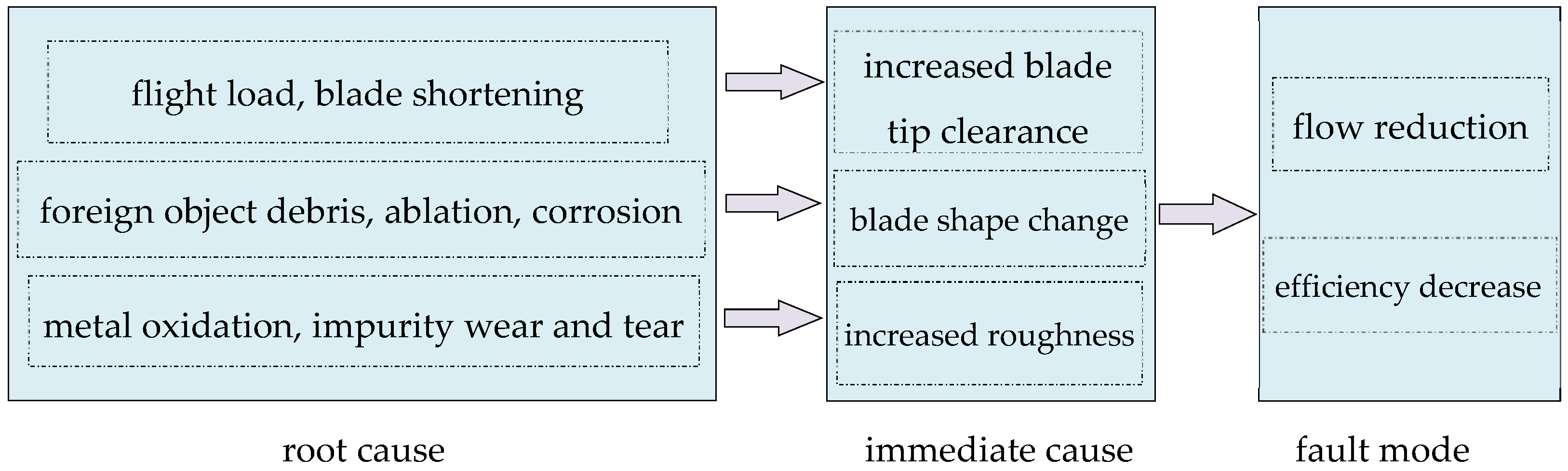
The primary factors causing changes in the components of an aeroengine’s gas path operating characteristics are illustrated in
Figure 14 [
67,
68,
69]. It is evident that regardless of the cause of the fault, for the gas path components, it will ultimately result in changes to their airflow and efficiency characteristics. Therefore, in this paper, the fault diagnosis focuses on these two parameters as the diagnostic targets.
In practical engineering applications, the most effective parameter tracking and estimation method is Kalman theory [
70] and its extended variant, the full-state observer Kalman filter. This approach estimates and tracks unmeasurable state variables based on system inputs and measurable outputs, making it particularly suitable for aircraft engine systems. If a nonlinear Kalman filter is adopted for parameter tracking in the onboard adaptive model, the underlying component-level model requires iterative solution using the Newton–Raphson method, incurring significant computational costs [
71]. In contrast, the augmented state-space model offers lower computational complexity, providing a foundation for real-time diagnosis in onboard applications. Therefore, this study employs a linear Kalman filter as the core algorithm for the fault diagnosis module in the onboard adaptive model, with its fundamental structure illustrated in
Figure 15:
The specific algorithm process is as follows:
- (1)
Prior state estimation:
State variables and covariance at the next time step are estimated using the current state variables and covariance. and are known quantities.
- (2)
Error covariance estimation.
- (3)
Calculation of the Kalman filter gain.
- (4)
State update.
- (5)
Error covariance update.
In summary, the linear Kalman filter consists of two main processes: first, the sequential estimation of system state variables and covariance, and second, the correction of the estimated values based on the residuals between the measured data and the system model output. The Kalman gain
K determines the weighting preference between the measured data and the system model output. When the Kalman gain is large, the estimation relies more on the measured data; conversely, when
K is small, the system model output has a greater influence on the state update. Additionally, after completing the state update and covariance update, the posterior state estimate is used as the prior estimate for the next estimation step [
72]. This recursive solution method ensures that all parameter estimates are based on the previous time step’s estimate without requiring access to the entire life-cycle operational data. When applied to the adaptive diagnostic model proposed in this study, this approach ensures real-time performance while maintaining high accuracy.
To ensure stable convergence of the Kalman filter estimation results, the target system must satisfy the observability condition. The necessary condition is that the number of measurable system parameters n must be at least equal to the number of gas path characteristic parameters to be estimated. That is, n ≥ dim(ΔPp) must hold. It follows that for the research model in this study, given the system matrix n = 8, the estimation requirements of the Kalman filter are satisfied, and the computational complexity of the algorithm meets the real-time requirements of the onboard model.
Based on the above analysis, the Kalman filter estimation equations for the system fault diagnosis module are designed as follows:
where
K is the Kalman filter gain,
K =
PUTnewR−1, and
P is the solution of the Riccati equation:
4.1. Improved Linear Kalman Filter
Considering that the conventional linear Kalman filter only takes the estimation deviation
at the current time step as an input, applying it directly to engine gas path characteristic parameter estimation over the entire flight envelope still results in estimation errors [
73]. Specifically, when the engine rapidly transitions between operating states (such as acceleration, climb, or altitude change), the tracking speed of the KF estimate following the true value change slows down or the amplitude becomes insufficient, inevitably generating certain dynamic tracking errors. After the state change ends, the error may not fully converge to zero but leaves a steady-state bias, namely residual(
k) =
y_actual(
k) −
y_predicted(
k|
k − 1). This is the deviation between the actual sensor measurement (
y_actual) and the measurement predicted (
y_predicted) based on the previous state estimate and model.
Furthermore, actual engines experience performance degradation during operation due to fouling, corrosion, and wear. This causes real engine parameters to deviate from the healthy baseline parameters established when the model was created. Health models based on the healthy baseline cannot characterize this slow, systematic parameter drift. The residual caused by model mismatch (especially the constant parameter drift induced by degradation) is persistent and relatively constant (or slowly varying). The KF’s instantaneous correction partially filters this out as noise or requires a long time to “fit” this drift through changes in , resulting in tracking lag and residual error. Moreover, when the engine operates in a prolonged condition, a slight model mismatch persists between the onboard linear model and the true operating system. After several update iterations, the Kalman filter converges to an “optimal” state estimate. However, this “optimal” state is not zero-error but maintains a constant deviation from the true value.
Therefore, there remains room for improving the accuracy of the fault diagnosis module. The original linear Kalman filter can achieve preliminary decoupling of the estimation loops for each parameter but does not fully achieve static decoupling between the estimation loops. To further enhance parameter tracking performance, an integral compensation module is introduced into the input of the original linear Kalman filter in this study. This approach applies continuous integral correction to the residual between the actual measured engine output and the theoretical output from the linear state-space model, effectively eliminating diagnosis errors. The improved Kalman filter is expressed as shown in Equation (58).
where
represents the excitation of the integral loop, and by adjusting the value of
, the dynamic and steady-state characteristics of the system estimation can be controlled.
It can be observed that, compared to the original fault diagnosis module, the input of the Kalman filter simultaneously includes the deviation Δy, which refers to the true measurable output performance parameter of the engine. In this context, it is characterized by the difference between the true output values of the nonlinear model under fault conditions and the steady-state values at the design point. is the deviation between Δy and the onboard model output estimate. When the estimation deviation of the Kalman filter becomes excessively large, the computation of the output residual Δy and the integral allows Δy to approach , ensuring that the onboard model can continuously and accurately estimate the variations in gas path characteristic parameters.
It can be seen that if the onboard model’s output becomes consistently lower (or higher) than the true value due to the engine’s long-term service-induced slow performance degradation, then η(t) will continuously accumulate positive (or negative) residuals over time, forming a signal that grows proportionally to the degradation amount. After adding this bias, a re-prediction is performed. η acts as a correction term applied to the model input, which is then fed into the Kalman filter for a prediction/update with bias compensation, analogous to the “PI (proportional + integral)” structure in classical control. Specifically, the reasons for using integration can be summarized as follows:
(1) Eliminating steady-state error: In linear systems, when there is a constant deviation between the system output and the model, relying solely on first-order state feedback or a single filter update will leave a constant bias term. To make the output error equal to zero at steady state, only by adding integration can this deviation accumulate over time, continuously applying increasing correction until the residual approaches zero.
(2) Counteracting slowly varying bias: Engine degradation is inherently a slow-varying process, not pure random noise. If treated merely as “process noise” (white noise), the Kalman filter will incorporate it into the state covariance but cannot guarantee the removal of the bias. Using an integral term specifically to track this slow drift enables continuous compensation over the long term. To apply the improved Kalman filter described by Equation (58) in the onboard model, the continuous equations must be discretized. For the continuous state-space model established in
Section 2,
Assuming that the system sampling period is
T, then
, and the state equation of the continuous system is expressed as follows:
Let
t = (
k + 1)
T,
t0 = 0, and the state equation can be further expressed as follows:
Thus, the expression for the discretized system is
where
.
The final expression for the discretized system is obtained as follows:
where
represents the dynamic error of the system, while
represents the system measurement noise.
In summary, the discrete formulation of the improved Kalman filter is given as
where
,
,
.
4.2. Full-Envelope Adaptability Mechanism
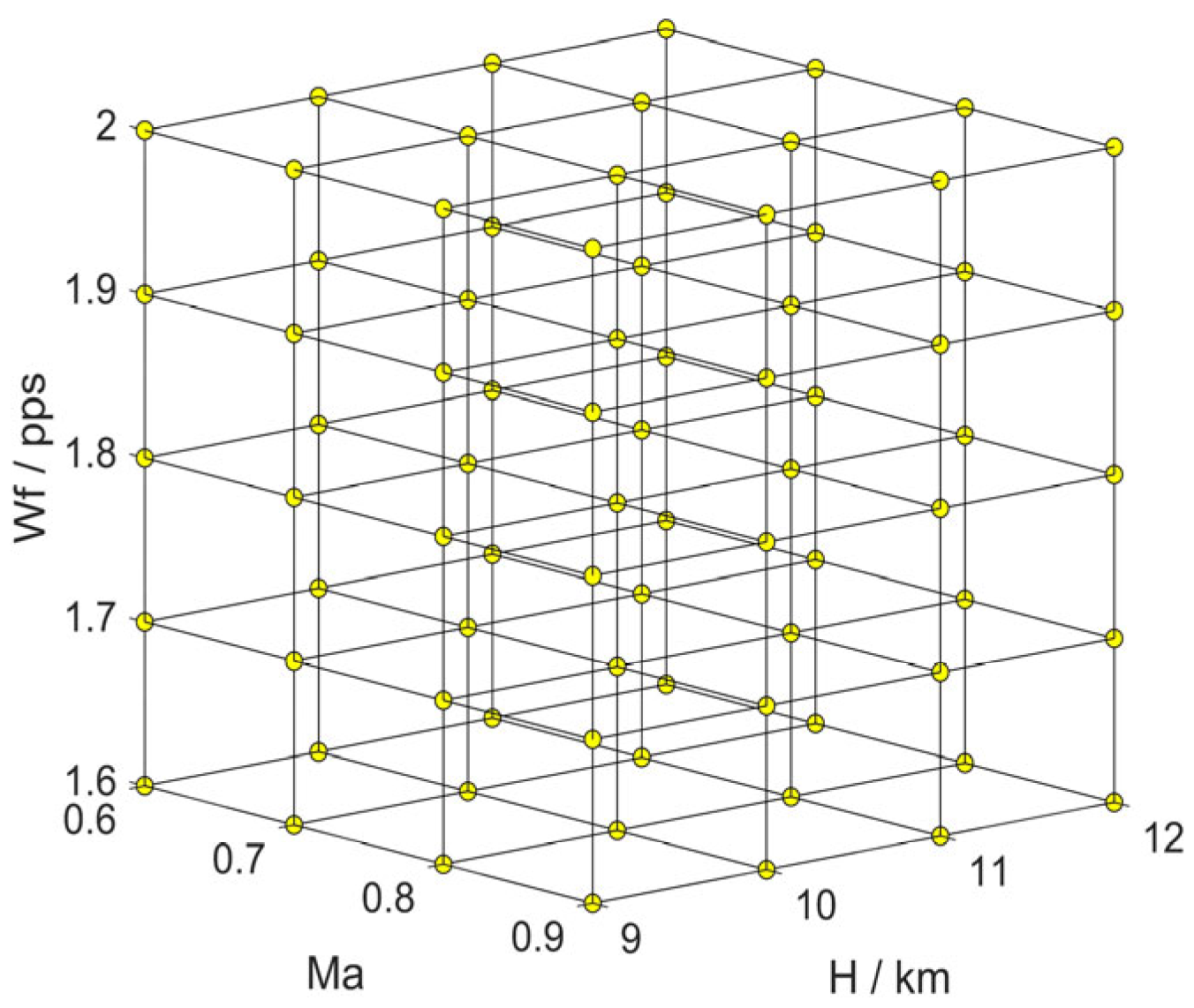
The operating conditions of a turbofan engine vary significantly due to changes in health status and flight conditions. The state-space model constructed for a single steady-state point exhibits limited applicability across the entire operational envelope throughout the engine’s lifetime. To address this issue, this section classifies flight conditions within the engine operating envelope based on altitude, Mach number, and fuel flow rate. A three-dimensional interpolation technique is then employed to interpolate between flight states, enabling the characterization of engine operating points across the full-envelope range. Let
H = 8–12 km and
Ma = 0.7–0.9, with intervals of Δ
Ma = 0.1 and Δ
H = 1000 m. The flight envelope is partitioned into 36 cubic subregions, with the endpoints designated as reference points, as illustrated in
Figure 16:
Building on the previous section, offline solutions for the augmented state-space models of 80 operational points within the flight envelope are computed, along with the corresponding linear Kalman filter sets {
Fi}. The gain matrix
Ki and the coefficient matrices of the augmented state-space models are stored in the onboard system. The steady-state reference point of this subregion is
Q11 = (
H1,
Ma1,
Wf1),
Q12 = (
H2,
Ma2,
Wf2),
Q13 = (
H3,
Ma3,
Wf3), Q
14 = (
H4,
Ma4,
Wf4), Q
21 = (
H5,
Ma5,
Wf5), Q
22 = (
H6,
Ma6,
Wf6), Q
23 = (
H7,
Ma7,
Wf7), Q
24 = (
H8,
Ma8,
Wf8) as shown in
Figure 17.
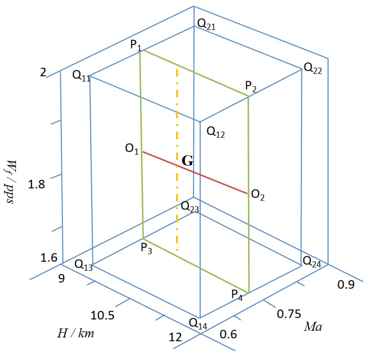
The algorithmic logic within the proposed onboard adaptive fault diagnosis model is as follows: First, based on the current altitude
H, Mach number
Ma, and fuel flow rate
Wf, the position of the operating point within a subregion is determined. Suppose the current operating point is
G, located in a specific flight region, as depicted in
Figure 18. Second, the eight reference points of this subregion are identified, and the corresponding stored state-space models and Kalman gain matrices are retrieved from the onboard system. The improved linear Kalman filter described in
Section 4.1 is then used to estimate the gas path characteristic variations at each reference point. Subsequently, linear interpolation is performed along the flight velocity
Ma to compute the estimated gas path characteristic variables at points
P1,
P2,
P3, and
P4.
where
f(x) represents the fault severity of the component under this operating condition.
Next, interpolation is conducted along the engine fuel flow rate
Wf to determine the estimated gas path characteristic variables at points
O1 and
O2:
Finally, interpolation is performed along flight altitude
H to obtain the estimated gas path characteristic variables at the operating point
G.
4.3. Experimental Results and Analysis
Under the operating conditions of Wf = 1.90 pps, H = 11,000 m, V = 0.8 Ma, and A8 = 862.88 in2, the onboard adaptive model is constructed based on the methodology proposed. The process noise matrix Q and measurement noise matrix R are selected as constant diagonal matrices based on the characteristics of the aeroengine system and engineering experience: , . After the system is initialized, the model calculates each output and state variable based on the actual altitude, speed, and fuel. To verify the comprehensive diagnostic capability of the proposed onboard model for various gas path faults, degradation factors are introduced into the gas path characteristic variables of the nonlinear model to simulate actual engine faults:
In
Table 3, the “time” column represents the simulation time at which fault factors are introduced. For example, “10/20” indicates that the two types of fault factors listed in that row are introduced at 10 s and 20 s of simulation time, respectively.
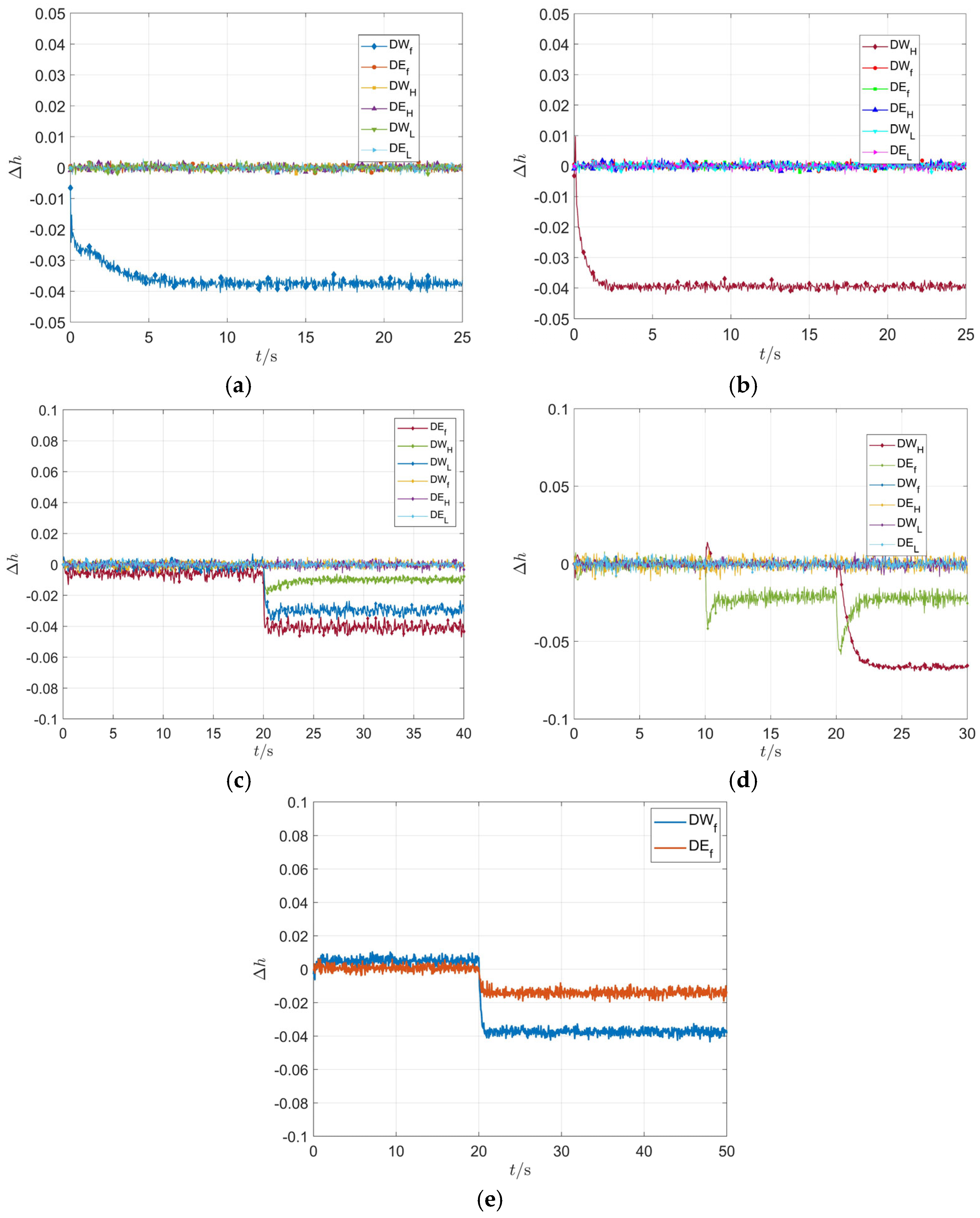
Figure 18 presents the engine gas path fault diagnosis results based on the proposed approach:
The results indicate that the proposed model can generally determine the fault severity and specific fault parameters of engine components within 5 s of simulation time. The tracking performance is good, accurately capturing the five introduced fault modes, and the final diagnostic values closely match the actual fault values.
Specifically,
Figure 18a,b show the fault diagnosis results for fan flow and HPC flow degradation of 3.8% and 4%, respectively. It can be observed that the system accurately identifies the faulty component and severity at approximately 1.02 s, begins tracking the gas path characteristics, and reaches steady state at approximately 2.52 s and 5.11 s. The identification remains accurate despite measurement noise and process noise.
Figure 18c shows the diagnosis results for simultaneous degradations of 1% in high-pressure compressor flow, 3% in low-pressure turbine flow, and 4% in fan efficiency at t = 20 s. The model accurately identifies the faulty components and their parameters at approximately 1.18 s, begins tracking the characteristic parameters, and reaches steady state at approximately 2.32 s. The identification remains precise.
Figure 18d presents the diagnosis results when the fan efficiency degrades by 2% at t = 10 s and the HPC flow degrades by 7% at t = 20 s. The model successfully identifies the first fault at 1.88 s; however, the subsequent fault introduction disturbs the tracking of the earlier fault, causing a temporary fluctuation with a peak magnitude of −0.058%. Nonetheless, the system restores the diagnostic value within 2.52 s and maintains accurate estimation performance. This disturbance is attributed to the nonlinear mapping between the working mechanisms of faulty components.
Figure 18e illustrates the diagnosis results when the fan flow and fan efficiency simultaneously degrade by 1% and 4%, respectively, at t = 20 s. The model accurately identifies the faulty components and parameters at 1.09 s and begins tracking the gas path characteristics, and the settling time is at approximately 2.12 s.
The root mean square error (RMSE) is used to quantify the diagnosis accuracy of gas path characteristic under different operating conditions within the flight envelope as shown in
Table 4:
It can be observed that the designed diagnostic model achieves an RMSE of less than 3% for each component. Among the selected test points, the lowest diagnosis accuracy is 2.953%, while the highest reaches 0.714%.
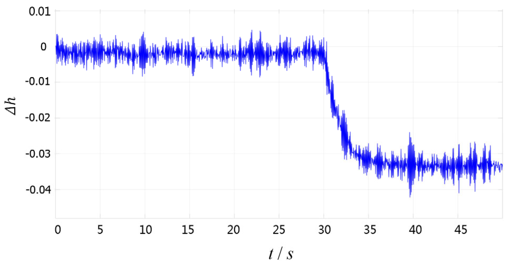
The classical sliding mode observer (SMO) is a traditional dynamic system that can estimate state variables based on measured values of external system variables and is also known as a state reconstructor. It has significant applications in state feedback techniques of control engineering. Therefore, in this study, SMO is also employed for fault diagnosis with the proposed aeroengine model. Under the same flight conditions, a gas path fault is injected at 30 s to simulate a 4% degradation in the fan airflow capacity of JT9D. The fault diagnosis of
WF is illustrated in
Figure 19.
The results indicate that under identical flight conditions, the estimated fan airflow capacity using the traditional SMO is 3.48%, and its noise filtering capability is relatively poor, leading to accumulated measurement noise. Compared with
Figure 18a, it is evident that the improved Kalman filtering algorithm proposed in this study significantly enhances accuracy and noise filtering performance over the traditional SMO-based fault diagnosis method. Regarding computational efficiency, as shown in
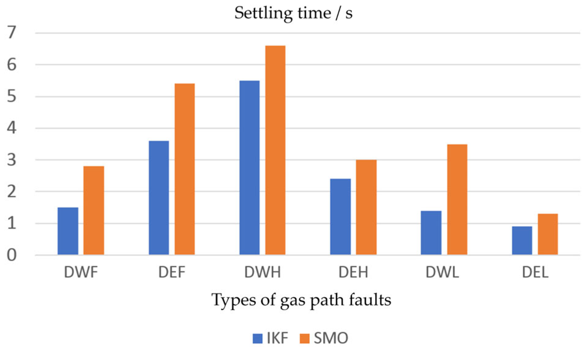
Figure 20, the settling time of the proposed approach is within 5.11 s, whereas SMO algorithm requires 8.21 s.
A 1% fault magnitude is injected at the 10 s simulation time into the fan gas flow rate, fan efficiency, HPC gas flow rate, HPC efficiency, LPT gas flow rate, and LPT efficiency of the nonlinear component-level engine model. The accuracy of the fault diagnosis is presented in
Table 5. It is evident that compared to the conventional SMO, the improved Kalman filtering algorithm still demonstrates superior performance across different fault modes, achieving a reduction in settling time by up to 2.11 s and an improvement in diagnosis accuracy by up to 3.619%.
Using operating condition 2 as the simulation condition, step excitations of different magnitudes are applied to the state variables of the nonlinear component-level engine model and the on-board adaptive diagnosis model. The comparison of the output responses of the two models is shown in
Figure 21:
The results demonstrate that the proposed model accurately tracks the gas path performance of the actual engine model, thereby enabling fault diagnosis. Moreover, the step response estimation errors of all state variables do not exceed 0.1%, meeting the precision requirements for practical engineering applications.
4.4. Performance Comparison of Existing Methods
To compare the algorithm proposed in this paper with existing methods (especially AI techniques, data-driven models, and tracking estimation algorithms similar to that in this paper), this paper conducted two experiments based on the following two dimensions: (1) adapting methods that cannot be directly compared with the proposed method, and comparing their fault diagnosis performance; (2) directly comparing the fault diagnosis performance of the proposed method with methods that can be directly compared.
- I.
Non-directly comparable methods
All methods ultimately aim to locate the faulty component and assess its severity. Therefore, for parameter tracking methods, the estimation error (RMSE) of Δ
p can be directly compared; for classification/probabilistic methods (Bayesian, SVM), their outputs are converted into fault severity estimates. For fault diagnosis methods that output discrete labels or probability distributions (Bayesian network, SVM classifiers), we map their outputs to continuous severity estimates using a standardized linear transformation:
where
Pk is the predicted probability for k-th severity level by model,
Sk is the standard severity value of k-th level (i.e.,
,
, …),
Smax is the maximum defined level (i.e.,
S5 = 5%), and
is the injected true fault value (i.e., −3.8%). This allows fair comparison of RMSE with parameter-tracking methods.
Hard classifiers like SVM output discrete labels directly (e.g., “Level 3”), lacking probability distributions and resulting in significant quantization errors. To facilitate comparison with the algorithm proposed in this paper, a three-step conversion method is provided:
- (2)
Confidence weighting improvement:
- (3)
Calculate confidence via decision function distance:
where
dk is the distance from the sample to the hyperplane of the k-th class and
α is a scaling factor (set to 1 in this paper).
Based on the above methods, the performance comparison of the proposed IKF, Bayesian Network, and Hybrid SVM methods for aeroengine fault diagnosis in this scenario is shown as
Table 6:
- II.
For algorithms comparable without conversion, the selected algorithms are as follows:
STF (Strong Tracking Filter);
ETKF (Event-Triggered Kalman Filter);
PGNN (Physics-Guided Neural Network), constrained to parameter estimation;
Traditional KF (baseline method);
- (1)
Fault modes: 1. single fault (fan flow decrease 3.8%, t = 0 s); 2. compound fault (ΔWfan = −4% & HPC ΔEfan = −1%, t = 20 s);
- (2)
Noise: Gaussian white noise (SNR = 10 dB);
- (3)
Flight envelope: H = 8–12 km, Ma = 0.7–0.9 (36 operating points).
- (4)
The performance comparison of the proposed IKF and comparable algorithms mentioned above is shown in
Table 7:
The PGNN convergence time is instantaneous during inference but requires 500-epoch offline training.
The experimental results show that in terms of fault diagnosis accuracy, for single faults, IKF achieves a lower RMSE (1.71%) than STF (2.05%) due to its integral compensation module suppressing steady-state errors. Under compound faults, IKF maintains the lowest RMSE (2.95%) as its 3D interpolation adapts to operating condition coupling effects. Regarding cross-condition adaptability, IKF demonstrates a 15.2% error increase rate—the optimal performance among all methods. In real-time processing, although ETKF has the highest computational efficiency (8.2 ms), its convergence time increases by 45% (due to event-triggering delays). IKF achieves the fastest compound fault convergence (5.11 s), with 12.4 ms inference time, meeting the 20 ms onboard system limit. Compared to Bayesian methods requiring probabilistic inference, our augmented state-space model reduces computational latency by 3.14 times through linearized Kalman filtering. Unlike hybrid SVM approaches, which highly depend on offline training data, our method achieves real-time adaptability via integral compensation and 3D interpolation.
While Bayesian and SVM methods focus on fault classification, we quantitatively compare their diagnostic precision by mapping discrete outputs to continuous severity levels. The proposed IKF achieves 1.14 times lower RMSE than SVM and 1.88 times lower than Bayesian methods, proving superior accuracy in quantifying fault severity. Notably, classification-based methods exhibit faster inference but cannot provide real-time parameter tracking capabilities. Recent adaptive AI algorithms focus on cloud-edge collaboration for fleet-level diagnostics. However, they require centralized data aggregation, violating onboard real-time constraints. Our method prioritizes embedded deployment with minimal data dependency.


