A Numerical Approach for the Integration of Sonic Boom Requirements into the Matching Chart

Abstract

The Matching Chart is a well-established tool in conceptual and preliminary aircraft design, providing a graphical representation of performance requirements based on wing loading (W/S) and thrust-to-weight ratio (T/W). It helps define a feasible design space while estimating key parameters such as thrust, maximum takeoff weight, and wing area. This paper presents a new numerical approach aimed at incorporating constraints related to sonic boom generated by supersonic aircraft in flight within the Matching Chart. The sonic boom constraint is derived from high-fidelity CFD simulations on similar case studies and atmospheric propagation models within a non-uniform atmosphere. The methodology is evaluated on an 80-passenger, Mach 1.5 aircraft, a configuration aligned with recent industry research. By integrating environmental and regulatory factors, this work enhances the Matching Chart’s applicability to enable more sustainable future supersonic aircraft design.

1. Introduction

In the last decades, there has been a rising interest in the development of a new generation of supersonic civil aircraft, as the demand for these configurations could potentially enable economically viable operations under certain conditions [1]. Different conceptual designs for future supersonic concepts are under evaluation [2,3,4], but to date, none of them have gone beyond the conceptual design phase. There are numerous environmental challenges in the reintroduction of commercial civil supersonic flights, such as the limits on pollutant emissions and noise impact, both on the ground and during cruise.

When an aircraft travels through the air at a speed exceeding the local speed of sound, it generates shock waves that propagate to the ground, producing what is commonly known as a sonic boom. This phenomenon represents one of the greatest challenges in high-speed aviation. These shock waves result in a loud and disruptive noise to an observer on the ground. Due to the annoyance that this phenomenon caused to the population during the development of Concorde, supersonic flight overland was prohibited in many countries, including the United States and Europe, since 1973 [5].

With the renewed interest in civil supersonic flights, it will be crucial to predict and mitigate the effects of sonic boom on the community on the ground. In the last decades, improvements in computational fluid dynamics (CFD) and atmospheric modelling have been made to enhance the prediction of sonic boom events and minimize the annoyance for future overland flights [6].

The National Aeronautics and Space Administration (NASA) has put significant effort in the development of the X-59, a supersonic demonstrator that has the goal of minimizing sonic boom annoyance on the ground to an acceptable limit [7]. The X-59 aircraft is designed to achieve a supersonic cruise at Mach 1.4 while minimizing the sonic boom, with the aim of limiting the perceived noise level to 75 dB or lower on Stevens’s MkVII Perceived Level of Noise scale on the ground [8]. This represents a substantial reduction compared to the sonic boom levels exceeding 100 PLdB typical of first generation of conventional civil supersonic airliners, such as the Concorde. The planned test campaigns aim to provide reference data that will help regulatory entities define limits of acceptability for future supersonic flights overland [9]. Future regulations on sonic booms rely on defining suitable acoustic metrics that correlate with public annoyance and on establishing acceptable threshold values. These metrics must account for the brief, impulsive nature of sonic booms and remain robust against atmospheric effects such as wind and temperature [10,11,12,13,14]. Clear, practical thresholds will guide regulations to balance aviation advancements with community comfort and environmental considerations. In order to do so, new methodologies and routines must be developed and seamlessly integrated into the design workflow to address these challenges early in the development process.

The conventional way to tackle the problem is to perform high-fidelity and computationally costly simulations, consisting, at first, of computational fluid dynamics (CFD) simulations in the proximity of the aircraft, and, subsequently, of a far-field atmospheric propagation to evaluate the effects of a non-uniform atmosphere, as is visible in Figure 1.

However, high-fidelity approaches are usually not easy to integrate within conceptual design processes, both because of the lack of detailed data to be used for the analysis at that stage and because of the time needed to run proper evaluations (CFD can take from days to weeks). A quick method to predict the sonic boom produced on the ground by an aircraft under study is notwithstanding crucial and more consistent to suit with the needs of the initial design process, allowing for an early assessment of the operational feasibility of the concept and for compatibility with environmental requirements. The definition of a low-fidelity approach is thus the right way to address this need, potentially benefiting from the results of high-fidelity methods applied to similar case studies, driving the definition of simplified correlations easily adaptable to the analytical and semi-empirical nature of the conceptual design process.

In fact, starting from high-level requirements such as payload capacity, maximum range, cruise speed, and altitude profiles, the conceptual design phase is mainly focused on creating an initial layout of the aircraft and estimating critical design parameters, including a preliminary mass breakdown and performance characteristics from aerodynamic and propulsion points of view. During this phase, the aircraft’s general configuration is outlined, including decisions on wing type, fuselage design, and engine placement, all of which can have a considerable impact on the sonic boom perceived on ground and whose contributions can be potentially captured by analytical expressions resulting from a synthesis of high-fidelity results from similar aircraft.

Supersonic aircraft design is a complex engineering challenge that involves aerodynamics, propulsion, materials, and structural considerations [15,16,17,18]. Unlike subsonic aircraft, which rely on traditional wing and fuselage configurations, supersonic aircraft must be designed to efficiently travel faster than the speed of sound while minimizing drag, managing heat, and mitigating sonic booms. Key design aspects include thin, swept, or delta wings to reduce wave drag, slender fuselages for smoother airflow, and specialized engine inlets to optimize air compression.

In order to help the designer facing these challenges, significant focus is placed on identifying or developing tools that can effectively visualize the design space, ensuring alignment with stakeholders’ expectations while adhering to design feasibility criteria.

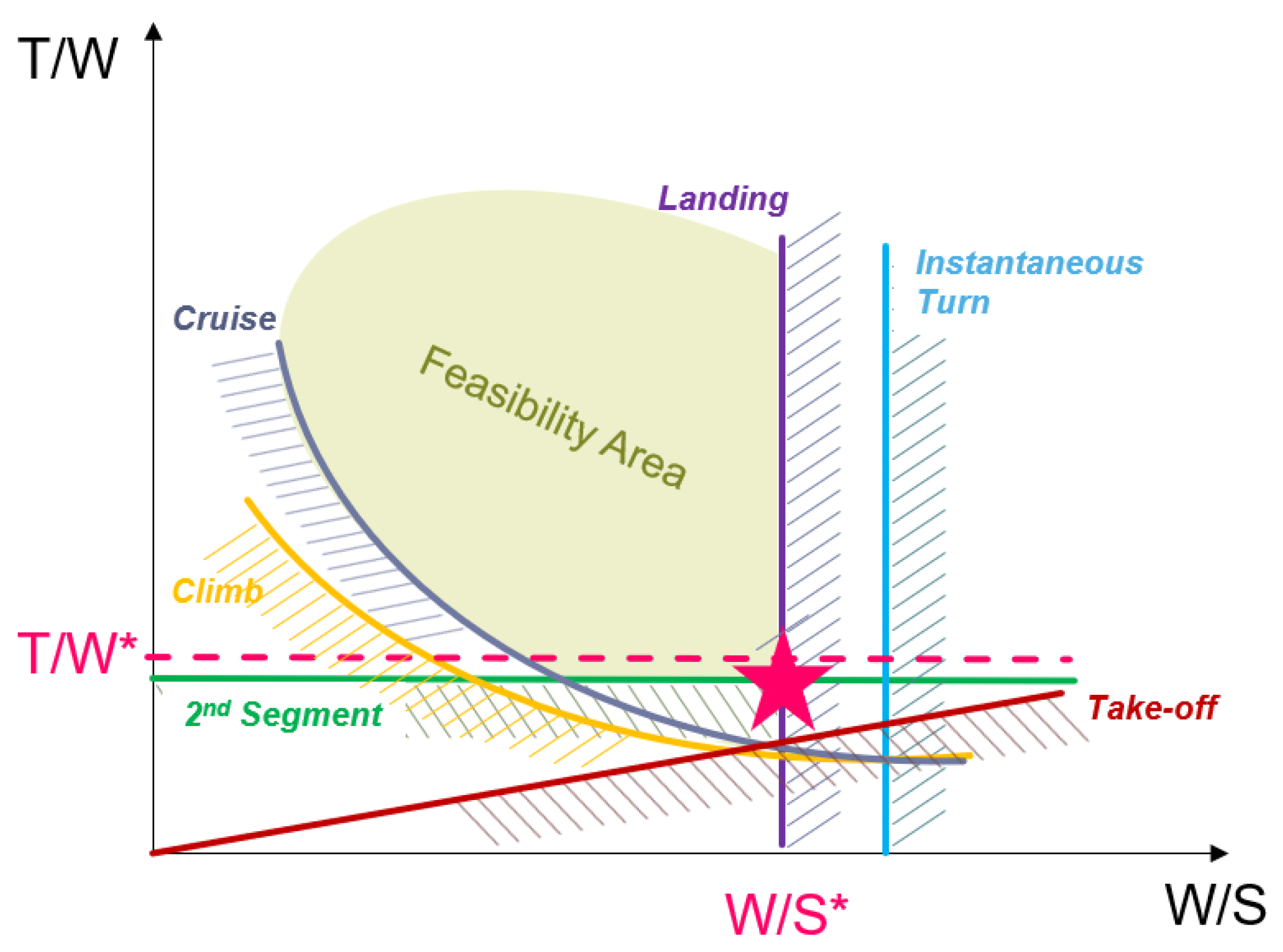
In the 1980s, NASA developed a streamlined methodology [19] to represent performance requirements during different flight phases in relation to the aircraft configuration, resulting in the creation of the so-called Matching Chart, which is a graphical representation that correlates the thrust-to-weight ratio (T/W ) to the wing loading (W/S) of the aircraft on a 2D chart. The proper definition of the most important performance of the aircraft, such as thrust T and lifting surface S with relation to weight W, is a fundamental aspect for the selection of the best design point to be evaluated as the baseline of the next phases of the project, but this traditionally tends to neglect environmental assessment.

This work tries to bridge this gap, including dedicated requirements in the Matching Chart to properly consider sonic boom limitations already within the conceptual design stage. The paper is structured as follows: Section 1 introduces the research context and objectives; Section 2 describes the case study, the Matching Chart tool, and the methodologies for the evaluation of sonic boom assessment requirement; Section 3 describes the high-fidelity sonic boom methodology; Section 4 presents the high-fidelity sonic boom results, while Section 5 presents the low-fidelity results, and finally Section 6 concludes with key findings, limitations, and future research insights.

2. Materials and Methods

2.1. Matching Chart Tool

Supersonic aircraft are designed to meet a broad set of performance requirements that extend beyond those of subsonic vehicles, driven by the challenges of sustaining flight at speeds exceeding the local speed of sound. A primary consideration in supersonic aircraft design is the management of wave drag, which dominates aerodynamic performance at high speeds. To minimize drag and improve efficiency, these aircraft often employ highly swept or delta wing configurations, in contrast to the high-aspect-ratio wings commonly found on subsonic aircraft. Beyond cruise performance, airport operations impose further design challenges. Supersonic aircraft typically require longer take-off and landing distances due to their higher stall speeds and reduced low-speed aerodynamic efficiency.

Addressing these challenges requires an integrated design approach that balances aerodynamic and propulsion efficiencies, as well as material advancements, while ensuring compliance with airport and regulatory constraints.

Conventional conceptual design methods typically start with the definition of high-level requirements in terms of payload/range coupling for a specific mission profile, characterized by several phases, and a specific Mach number in cruise at a certain altitude. The hypotheses on the type of propulsion plant used and on the category of the aircraft are also important to estimate first guesses of data about the Specific Fuel Consumption (SFC) as well as about basic aerodynamic characteristics. Then, an iterative approach is usually adopted, as specified by [20,21,22], where take-off mass is computed according to a mass build-up approach, where empty mass is a function of configuration parameters, while fuel mass is obtained by means of analytical equations describing the fuel consumption in the different phases. Breguet range correlation [23,24] is generally adopted in the cruise phase, together with other phases at constant altitude, while the fuel used in climb or cruise legs can be computed either by referring to reference values for the ratio between the mass at the end and at the beginning of the specific phase, as [21] suggests, or by adding factors to introduce a margin for the equivalent all-out range, as prescribed by [22]. The overall iteration process is controlled by looking for the convergence of final mass, iteration by iteration.

The introduction of performance requirements for the different phases also allows deriving the required wing surface to sustain the aircraft during flight, as well as the required thrust to balance drag forces at different conditions. This is performed by means of the Matching Chart, which associates thrust requirements and wing surface values for each iteration to the take-off mass.

A graphical representation of a typical Matching Chart is visible in Figure 2, where performance requirements representing equilibrium equations in different phases are shown as curves or lines in the 2D space, while the feasibility area is shaded in green. The design point (star and related values on the axis) is here represented in a situation where priority is given to the maximum allowable wing loading (i.e., minimum required wing surface for a given take-off mass, typically in stall or landing conditions).

Through the use of this tool, upon convergence, it is possible to select specific values of $T/W$ and $W/S$, and thus to identify a single configuration to be used as the baseline for further investigations. This approach streamlines the aircraft sizing process by allowing different flight conditions and propulsion performance to be evaluated in a single plot. To ensure comparability, the equations are adjusted to reflect equivalent conditions at sea level. The viable design space (feasibility area) is defined depending on the different curves, as Figure 2 suggests, while the design point usually corresponds to the location where the minimum $T/W$ is achieved, maintaining a consistent $W/S$ value. Available thrust shall then be slightly higher, considering a proper margin (dashed pink line).

This approach, originally proposed by [19], is still valid today, being flexible enough to support different kinds of aircraft design studies [26,27], with proper updates to tune the method as a function of the aircraft category.

For this specific work, the inclusion of a sonic boom requirement at the conceptual design stage is imperative, as no prior efforts have systematically addressed this aspect, leading to a lack of early consideration for sonic boom constraint. As described in the following sections, this task is performed by statistically modeling bow shock overpressure based on high-fidelity simulations. By including the sonic boom requirements in the Matching Chart, it becomes possible to assess early-on the trade-off between performance goals and noise limitations, allowing for a more comprehensive and practical design process.

2.2. Case Study

A Mach 1.5, 80-passenger configuration was chosen as a case study due to its balance between speed, capacity, and feasibility for future supersonic travel. This design is tailored for high-demand business routes, offering substantial time savings while maintaining economic feasibility for airlines. With advancements in aerodynamics and noise reduction technologies, Mach 1.5 becomes a practical and viable cruising speed. This configuration represents a realistic step toward reintroducing commercial supersonic flight within operational and environmental constraints [28,29,30].

The reference aircraft used as a case study was inspired by the work performed in [31], where the characterization of a viable propulsion system for a similar aircraft is described. A re-design of the aircraft to ensure higher payload was carried out exploiting the proprietary tool ASTRID-H, already tested for a wide range of supersonic aircraft design exercises in [32]. This tool enables users to transition from the statistical analysis of guess data and design space identification to the geometric characterization of vehicles, ensuring proper integration of key subsystems. It incorporates widely used mathematical models into algorithms designed to tackle the complexities of high-speed vehicle design.

The reference case study evaluated in this paper has the following high-level requirements.

• Cruise Mach number: 1.50
• Payload: 80 passengers, 110 kg each
• Range: 6000 km
• Cruise altitude: 18,000 m (59,000 ft)
• Maximum peak overpressure at ground level: $\Delta p_1<50$ Pa
• Absolute value between peak overpressure and peak expansion at ground level: $|\Delta p_1| + |\Delta p_2|$ $<100$ Pa

The peak overpressure requirement of 50 Pa is justified to ensure that the sonic boom remains within potential future limits for human tolerance and regulatory compliance with noise exposure standards for supersonic flight. Moreover, the inclusion of a peak-to-peak amplitude requirement allows for constraints on the entire pressure signature, including the negative phase, thereby providing a more comprehensive control over the boom perceived impact.

As a result of the iteration process, the sketch and the mass breakdown of the vehicle are reported in Figure 3 and

Table 1. Case study geometric and performance data.

Characteristic	Value
MTOW	148,970 [kg]
Payload	9660 [kg]
OEW	66,485 [kg]
Wing area	358.79 [m2]
Wingspan	25.85 [m]
Aspect ratio	1.86 [-]
MAC	20.88 [m]
Sweep angle	64.24 [deg]
Root chord	31.22 [m]
Tip chord	1.87 [m]
Tail area	70.77 [m2]
Fuselage length	57.78 [m]
Fuselage width	3.01 [m]
Required Thrust	493. 6 [kN]

, together with relevant characteristics.

In Table 1, MTOW is the maximum take-off weight, OEW is the operative empty weight, and MAC is the mean aerodynamic chord.

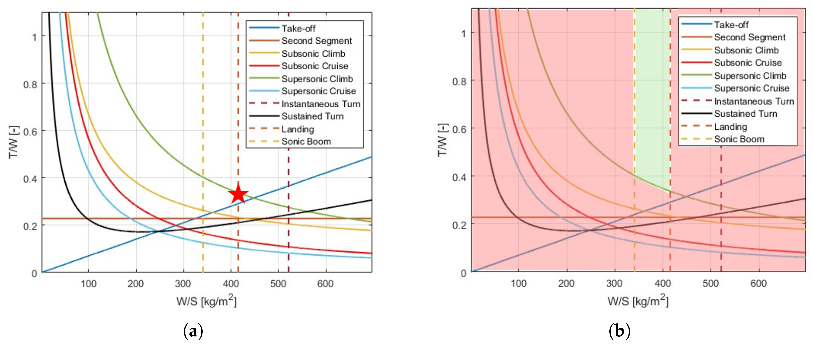
The resulting Matching Chart for the converged solution is reported in Figure 4, where a $T/W$ of around 0.34 and a $W/S$ of 415 kg/m² are derived for the design point. Similarly to what qualitatively shown in Figure 2 the design point (picture on the left) is chosen at the lowest possible value of thrust-to-weight ratio, corresponding to the maximum allowable wing loading to satisfy landing requirement (bottom right corner of feasibility area shown in the picture on the right).

2.3. Sonic Boom Assessment: Low-Fidelity Method

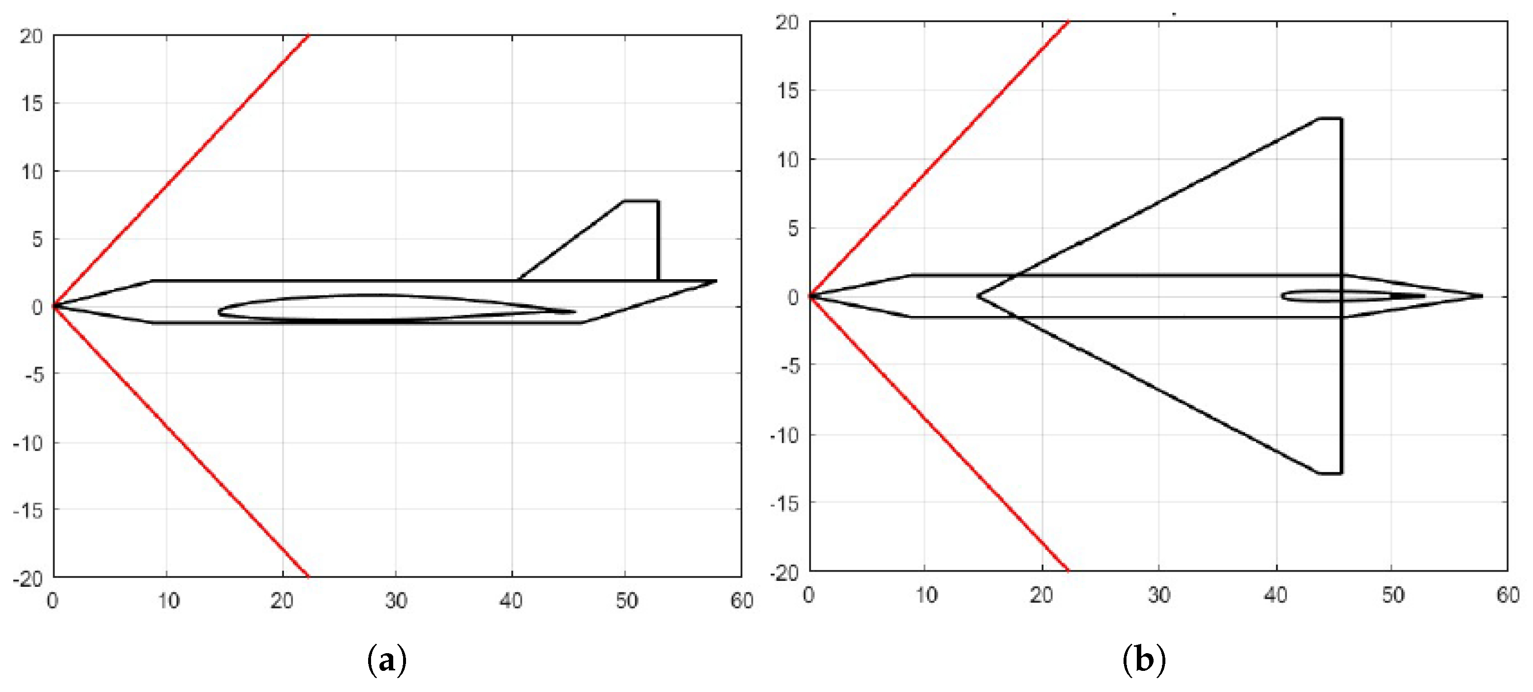
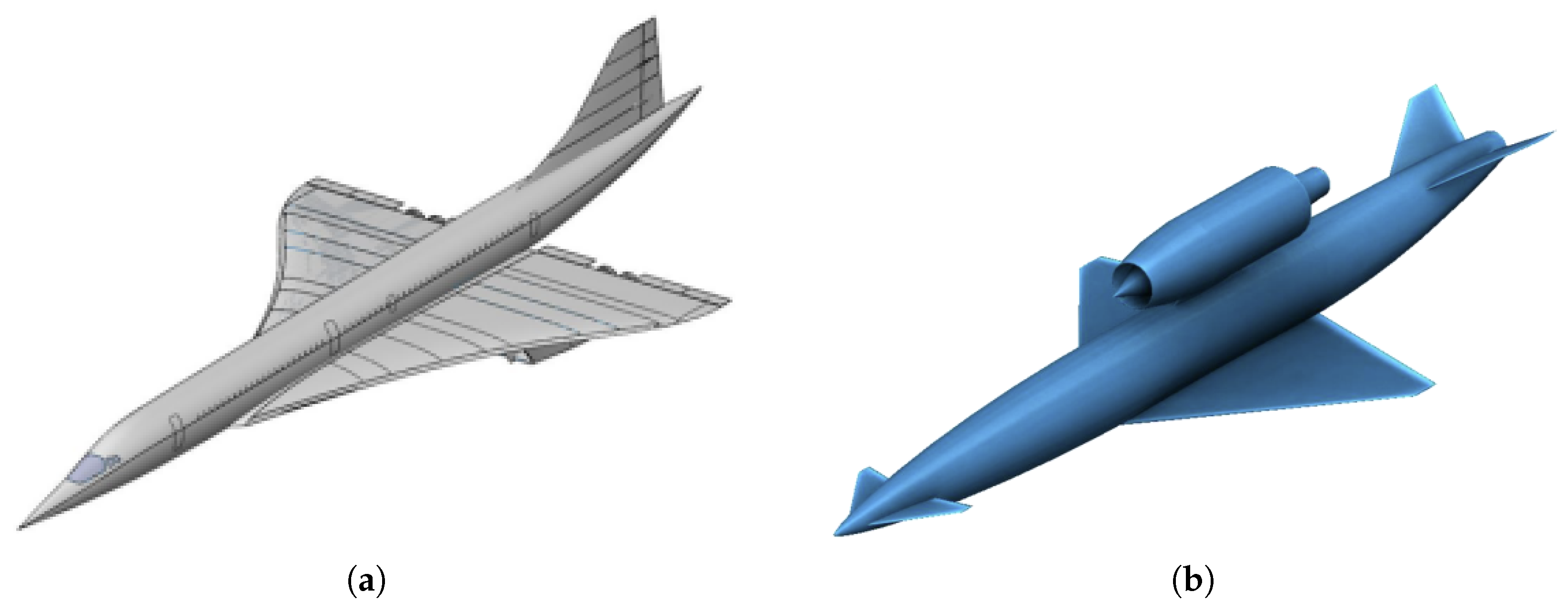
The low-fidelity method described here involves the use of a statistical basis to estimate the peak pressure in the ground pressure signature. The aircraft included in the statistical population are two, although the number of collected pressure signatures is greater. This is because, for the same aircraft, numerous flight scenarios were considered, and the pressure signature on the ground is strongly influenced by the reference flight condition. Specifically, it is related to the Mach number, altitude, and angle of attack, as well as atmospheric conditions. The aircraft that were simulated are the so-called Case Study 1 ($CS1$) and Case Study 2 ($CS2$), as shown in Figure 5, analyzed within the H2020 European Project MOREandLESS (MDO and Regulations for Low-boom and Environmentally Sustainable Supersonic aviation) [33]. The $CS1$ vehicle is a Concorde-like commercial Mach 2 aircraft very similar to the Aérospatiale-BAC Concorde [34], with minor differences in the wing shape and propulsion plant. The main geometrical quantities are identical to the previous configuration and are shown in

Table 2. CS1 geometric information.

Characteristic	Value
Aircraft length	62.30 m
Wing surface	358.3 m2
Wingspan	25.6 m
root chord	27.66 m
Maximum Take-off Weight	179,000 kg
Design range	6500 km
Design fuel weight	85,289 kg
Thrust to weight ratio	0.4
Wing loading	494 kg/m2

.

On the other hand, the $CS2$ aircraft [35] is a vehicle concept studied by Reaction Engines Ltd. (Oxfordshire, UK) for use as a test bed for SABRE—the Synergetic Air-Breathing Rocket Engine [36]. The ultimate design goal for demonstrating the SABRE air-breathing technology is to achieve Mach 5 at altitudes exceeding 20 km (approximately 70,000 feet). The vehicle features a slender fuselage to minimize drag, and a low-aspect-ratio delta wing, enabling both low- and high-speed flight. It also features a pair of canards (or foreplanes) for pitch control, along with a pair of vertical stabilizers at the rear.

The $CS2$ configuration employs multiple propulsion systems. The primary air-breathing propulsion system, housed within a single nacelle, is mounted on the dorsal surface of the fuselage to serve as a testbed for the experimental SABRE technology. Additionally, a secondary propulsion system—a conventional rocket engine utilizing liquid hydrogen and liquid oxygen as propellants—is installed at the rear of the fuselage.

Additional information about the $CS2$ geometry is provided in

Table 3. CS2 geometric information.

Characteristic	Value
Aircraft length	24.50 m
Wing surface	40.00 m2
Wingspan	9.00 m
Root chord	7.50 m
Tip chord	1.00 m
Canard root chord	2.00 m
Canard tip chord	0.50 m

, based on a set of assumed main characteristics.

Table 4. Statistical database used for case study.

	M [-]	h [km]	$\mathit{\alpha }$ [deg]	A.length [m]	W.span [m]	W.surface [m2]	$\mathbf{\Delta }{\mathit{p}}_1$ [Pa]	$\mathbf{\Delta }{\mathit{p}}_2$ [Pa]
CS1	2	17.5	0	61.66	25.9	358	42.61	−45.48
CS1	2	17.5	2	61.66	25.9	358	59.85	−51.78
CS1	2	18	0	61.66	25.9	358	43.09	−49.31
CS1	2	18	−2	61.66	25.9	358	25.85	−47.32
CS1	2	18	2	61.66	25.9	358	65.59	−53.62
CS1	2	18	4	61.66	25.9	358	85.70	−68.94
CS1	1.75	18	0	61.66	25.9	358	39.74	−46.44
CS1	1.75	18	−2	61.66	25.9	358	26.81	−45.00
CS1	1.75	18	2	61.66	25.9	358	62.73	−52.19
CS1	1.75	18	4	61.66	25.9	358	74.69	−55.06
CS1	1.5	18	0	61.66	25.9	358	35.43	−46.44
CS1	1.5	18	−2	61.66	25.9	358	26.33	−43.09
CS1	1.5	18	2	61.66	25.9	358	60.32	−51.71
CS1	1.5	18	4	61.66	25.9	358	75.18	−60.81
CS2	1.2	11.3	0	24.5	9	40	37.82	−58.89
CS2	2	11.3	0	24.5	9	40	56.49	−65.59
CS2	2	28	0	24.5	9	40	9.09	−10.05

presents the dataset used as input for the low-fidelity method. It was built by collecting data from high-fidelity simulations carried out for various flight conditions of the two aircraft presented. See Section 4 for details.

In Table 4, A.length is the aircraft length, W.span is the wingspan, W.surface is the wing surface, h is the altitude of the high-fidelity simulation, and $\alpha$ is the angle of attack.

2.3.1. Linear Regression

The primary objective of the mathematical model developed within the low-fidelity method is to identify the relationships between aerodynamic and geometric variables (inputs) and the positive and negative peaks of the ground pressure signatures (outputs). The chosen model is a multiple linear regression that can be written as follows:

$$y={\beta }_0+{\beta }_1{x}_1+{\beta }_2{x}_2+\dots +{\beta }_i{x}_i+ϵ$$

(1)

where y represents the dependent variable, $x_1,x_2,\dots ,x_i$ are the linearly independent variables, ${\beta }_0$ is the intercept (the value of y when all x values are equal to 0), and ${\beta }_1,{\beta }_2,\dots ,{\beta }_i$ are the regression coefficients (parameters indicating the unit effect of each independent variable on the dependent variable). Finally, $ϵ$ represents the statistical error term. The model estimates the coefficients by minimizing the sum of squared differences between the observed and predicted values, typically using the least squares method. It assumes that the relationship between the variables is linear, that observations are independent, that errors have constant variance, and that residuals follow a normal distribution. The aim is to determine the relationship between the variables by assessing how each independent variable influences the dependent variable, make predictions on new data using the discovered relationships, and interpret the system by providing an equation that clearly describes it.

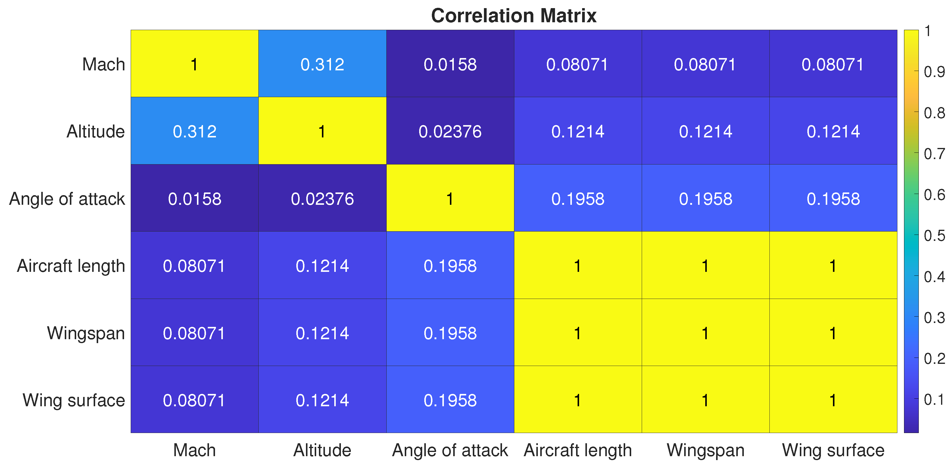
2.3.2. Correlation Analysis

The independent variables are six in total, plus two dependent variables, namely the pressure peaks. As a result, two equations must be derived, each linking the six inputs to a single output. Among the independent variables, three pertain to the aircraft dimensions and exhibit interdependencies. To enhance model accuracy, a correlation analysis is performed to assess whether any of these variables can be excluded. This analysis was conducted using the MATLAB 2024R1 corrcoef function [37]. The input data consists of a matrix where each column represents a variable and each row corresponds to an observation. The dataset includes the same aircraft concepts introduced in Section 2.3 for the low-fidelity method. The dimensional parameters considered are aircraft length, wingspan, and wing surface, while the flight condition parameters include Mach number, altitude, and angle of attack. The function calculates the Pearson correlation coefficient [38] between variable pairs and returns a symmetric correlation matrix. The coefficient ranges from −1 (perfect negative correlation) to 1 (perfect positive correlation), with 0 indicating no correlation.

Figure 6 presents the heatmap of this correlation matrix. As expected, for aircraft within the same category, strong correlations exist among aircraft length, wingspan, and wing surface. Additionally, other variables show partial correlations, mainly due to the limited dataset size. For optimal linear regression performance, only one of these three highly correlated independent variables is retained. Wing surface is chosen because it is a key sizing parameter and a direct output of the Matching Chart, while aircraft length and wingspan are excluded.

2.3.3. Mathematical Model

All the parameters necessary for the application of the mathematical model are defined and constitute the two matrices X and Y.

• Inputs (X): Mach, altitude, angle of attack, and wing surface;
• Outputs (Y): $\Delta p_1$, the positive pressure peak, and $\Delta p_2$, the negative pressure peak.

Firstly, the model adds a unit column to the inputs matrix X, modelling the regression intercept. In the second step, it performs the linear regression, computing two linear vectors $b_{1linear}$ and $b_{2linear}$, for $\Delta p_1$ and $\Delta p_2$, respectively, through the least-squares method:

$$b={\left(X^{T}X\right)}^{-1}{X}^{T}y$$

(2)

These vectors store the $\beta$ coefficients of the resulting equations. Subsequently, the model calculates the predicted values of $\Delta p_1$ and $\Delta p_2$, denoted as $y_{{\mathit{pred}}_1}$ and $y_{{\mathit{pred}}_2}$, by multiplying the previously estimated coefficients with the input matrix X. Finally, the model evaluates the residual sum of squares (SSE) and the total sum of squares (SST) through the following computations:

$$SSE=\sum _{i=1}^m{(y_i-y_{pre{d}_i})}^2$$

(3)

$$SST=\sum _{i=1}^m{(y_i-\overline{y})}^2$$

(4)

where $\overline{y}$ is the mean of the observed values Y. From these parameters, the coefficient of determination ($R^2$) is derived, which measures the goodness of fit of the model, taking values between 0 and 1. This coefficient can be expressed as follows:

$$R^2=1-{\displaystyle \frac{SSE}{SST}}$$

(5)

Lastly, the results are visualized as the equations corresponding to $\Delta p_1$ and $\Delta p_2$ in Equations (7) and (8) (Section 5).

3. Sonic Boom Assessment: High-Fidelity Method

High-fidelity techniques are generally used to study and characterize the flow around a supersonic or hypersonic object due to the strong non-linearities and interactions. These techniques are generally divided into two different domains: the near-field region, which is described in Section 3.1 and is the area in the proximity of the aircraft where the three-dimensional fluid effects are evaluated via CFD, and the far-field domain, which identifies the impact of a non-uniform stratified atmosphere, as briefly described in Section 3.2. In the proximity of the configuration, the different shock waves create a detailed pressure signature that accounts for every detail of the aircraft geometry and shock interactions.

3.1. Near-Field Region

Numerous improvements have been made in the last twenty years in the computation of shock waves via computational fluid dynamics (CFD) [39,40]. Since 2014, NASA has been hosting the AIAA Sonic Boom Prediction Workshop, which aims to define the state-of-the-art in the numerical prediction and propagation of sonic booms [41,42,43]. In the proximity of a supersonic aircraft, aerodynamic effects significantly influence shock wave formation. At greater distances from the configuration, the impact of refraction, resulting from a non-uniform and dynamic atmosphere, becomes more pronounced. The near-field simulations were conducted using the commercial software ANSYS Fluent 2023 R2 [44], which employs an unstructured finite-volume approach, with gradients computed using a Green–Gauss method. Fluent uses an adaptive Courant–Friedrich–Lewy (CFL) number as a convergence strategy, and all simulations were performed neglecting the turbulence models, solving the inviscid Euler equations with the assumption of an ideal gas model for the air. Neglecting the turbulent characteristics of the flow could potentially result in an incomplete capture of shock-boundary layer interactions, which may influence the shock strength and position. However, the computational cost required for Euler simulations is lower compared to Reynolds-Average Navier–Stokes RANS equations since they do not require turbulence modelling or the resolution of boundary layers. In fact, previously published work in the literature indicates the computational cost advantage of neglecting turbulence models when predicting the shock waves emitted by a supersonic or hypersonic configuration [45,46,47,48,49,50]. In this paper, a series of steady-state simulations based on the Euler equations was carried out to model the near-field flow under cruise conditions, where no significant unsteady phenomena are expected. Euler simulations are sufficient for preliminary sonic boom analyses, where the goal is to assess the behaviour of the simulated configuration. In later stages of the project, simulations with higher computational costs can be considered. In particular, the second Sonic Boom Prediction Workshop [42] highlighted that grid dependency in Eulerian simulations without viscous terms was minimal, with negligible impact on ground-level propagation. In this work, a similar grid discretization strategy is applied, and the simulations are performed under steady-state conditions, assuming a simplified flow regime in which viscous effects are neglected, and turbulence is omitted. The air phase is modelled as an ideal gas using the corresponding equation of state. The inlet boundary is specified as a pressure far-field condition, with pressure and temperature set to the free-stream values, while the outlet is defined by a pressure outlet boundary condition. Due to the geometric and flow symmetry of the configuration, only half of the aircraft was modelled, and a symmetry boundary condition was imposed along the longitudinal plane to reduce computational cost. Additionally, all remaining external boundaries of the mesh—excluding the inlet and outlet—were modelled as slip walls to confine the domain without introducing significant flow disturbances. Further details can be found in the work by Graziani et al. [45].

Numerical schemes play a crucial role in translating equations from continuous models to the discrete one, which can be implemented in computational solvers. In the context of the supersonic Mach numbers studied here, the Fluent software 2023R2 offers the second-order upwind implicit ROE scheme with flux-difference splitting (ROE-FDS), as described by [51,52]. The ROE-FDS method is built upon the Roe scheme, which approximates a Riemann solver for hyperbolic conservation laws. One of the key advantages of the ROE-FDS scheme is its ability to consistently split fluxes in alignment with their corresponding flux method’s eigenvalues. This feature is particularly beneficial for accurately capturing discontinuities, such as shocks, which are commonly encountered in high-speed flow simulations. The scheme ensures that the physical behaviour of the flow, especially in regions with steep gradients or discontinuities, is well-represented and stable in the numerical solution.

The computational grid is composed of two different regions, as can be seen in Figure 7: firstly, an unstructured grid in the vicinity of the aircraft designed as a half cylinder, followed by a structured grid aligned with the Mach angle $\mu$ for the whole domain of the numerical simulation. The length of the domain in the vertical direction is equal to 3.5 times the characteristic length of the aircraft. The numerical elements are tetrahedral in the unstructured domain, hexahedral in the structured, and pyramidal to connect the two zones, with a total number of elements for the two configurations of around 20 million. The ambient pressure field is homogeneous, with initial conditions for the free-stream pressure and temperature.

As it is common in CFD simulations, the ambient pressure field is homogeneous with a constant initial condition for the free-stream pressure for both the inlet and the outlet parts. The sonic boom signal however, which travels from an altitude of several kilometres towards the ground, is also affected by the gradients of sound speed and wind during propagation in the atmosphere. To account for these effects of a non-uniform medium, the far-field propagation is performed with a different modelling approach, which is described in the following section.

3.2. Far-Field Region

In this paper, the propagation of the shock waves from the reference altitude to the ground was performed with PCBoom solver, version 7.1, developed by NASA [53,54,55,56,57]. The solver applies full three-dimensional ray tracing based on geometrical acoustics, and it predicts sonic boom waveforms and footprints on the ground for different flight scenarios. It was widely used and validated during the latest AIAA Sonic Boom Prediction Workshops [58,59,60]. The waveforms on the ground are predicted by resolving the Burger equation, selecting the Enhanced Burger solver, which accounts for atmospheric absorption and full wind effects [53]. In addition, Doppler effects are included via frequency shifting based on the motion of the medium relative to the ground reference frame.

In the modelling of sonic boom propagation, a reflection factor of 1.9 has been adopted as a simplification to account for the interaction of the boom wave with the ground. This value is based on the assumption of a perfectly flat and rigid surface, which allows for a straightforward estimation of the reflected wave contribution. While in reality, ground impedance, terrain roughness, and atmospheric conditions can influence the actual reflection characteristics, as highlighted by [61]. Within this work, only the value of peak pressure of the propagated near-field pressure signature is evaluated as the output of the propagation module, without any consideration related to different acoustic metrics or primary carpet width. In accordance with the definition of the conceptual design stage, peak pressure has been accounted for to enable efficient early-stage assessment. Another important atmospheric mechanism, which is neglected in this study, is the role of atmospheric turbulence in the planetary boundary layer. The turbulence can have a large impact on the ground signature and introduces variance to the associated sonic boom loudness [11,13].

3.3. Applicable Atmosphere

Accurately predicting sonic boom propagation requires careful consideration of atmospheric conditions. Factors such as temperature, humidity, wind, and pressure gradients affect the way shock waves travel, refract, and dissipate over distance. These variations influence boom intensity, extension of the carpet, and loudness metrics, which are critical for environmental assessments and community response evaluations. The International Standard Atmosphere (ISA) is commonly used to simplify and standardize the variation in atmospheric parameters [62], such as a vertical temperature gradient in the troposphere being constant at −6.5 K/km, and the absence of winds both in the frontal and lateral directions. The ISA definition was extended to include a standardized humidity profile, as outlined in ANSI S1.26 Annex C [63] and proposed by the organizers of the Sonic Boom Prediction Workshop. This humidity profile is incorporated in the analysis of the ISA atmosphere. Nevertheless, due to the assumptions of no winds in both frontal and lateral directions, alternative atmospheric profiles were selected to comprehensively characterize the shock waves on the ground generated by the two analyzed configurations. Specifically, realistic profiles from the second and third Sonic Boom Prediction Workshops (SBPW2, SBPW3, respectively) were chosen.

As previously stated and highlighted Figure 8 and Figure 9, the International Standard Atmosphere does not define wind profiles.

The first selected profile in the SBPW3 will now be refereed as “Case 1 SBPW3 ”, and it represents an atmospheric condition that allows a wide range of azimuth angles to reach the ground for an aircraft flying eastward. The second profile, named “Case 2 SBPW3”, corresponds to an atmospheric state that produces a particular broad sonic boom footprint for an eastward-flying aircraft. Lastly, the atmospheric profile from the second Sonic Boom Prediction Workshop for the aircraft body was used and referred to as “Case 3 SBPW2”.

4. Sonic Boom Assessment: High-Fidelity Results

This section highlights the high-fidelity results that are the drivers for the development of the low-fidelity database. The high-fidelity results are obtained first with computational fluid dynamics (CFD) in the near-field domain, and then the propagated pressure signature on the ground is obtained with a dedicated propagation tool, following the approach evaluated in Figure 1.

Firstly, CFD results will be evaluated in Section 4.1, and then the propagated results will be shown in Section 4.3. The pressure signature is usually evaluated at a distance from the aircraft that is proportional to length of the vehicle itself. Named $H/L$, the ratio between the distance of extraction and the characteristic length of the aircraft, the pressure variation is extracted from the flow field at specific values that would be the input within the propagation module. 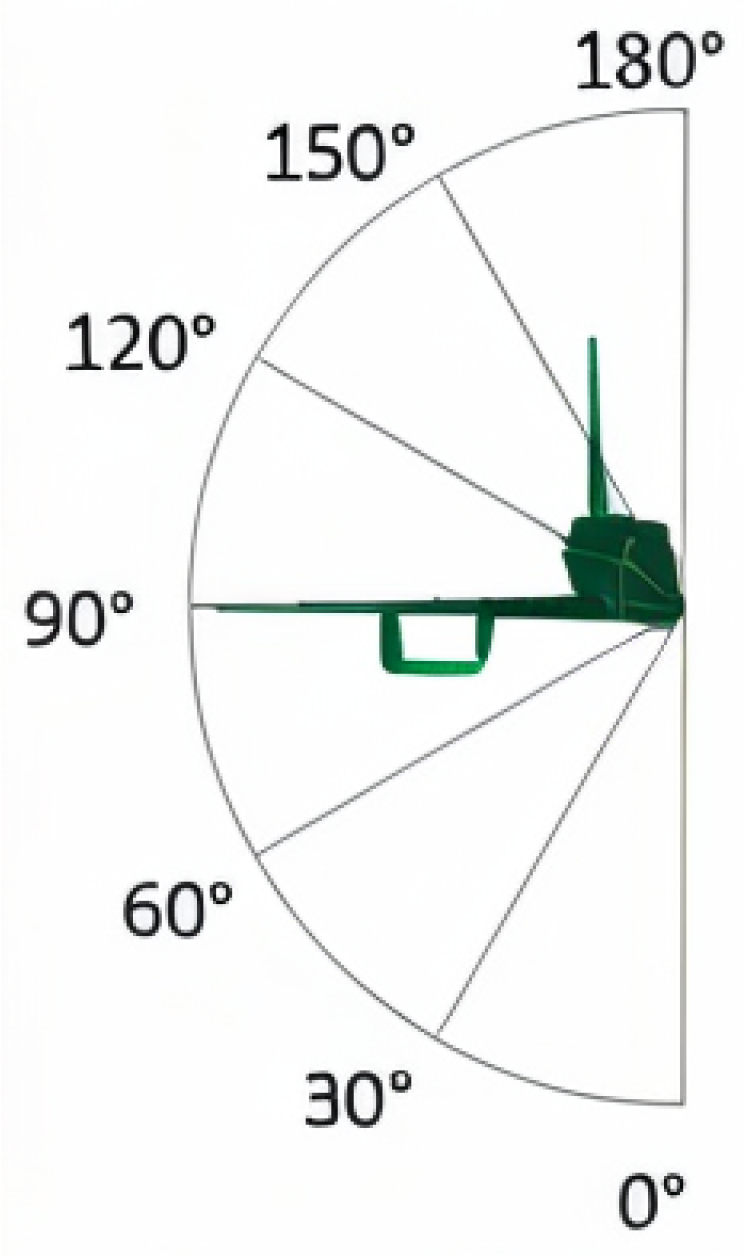Within this work, the extractions were made at $H/L=1$ and $H/L=3$; so, the CS1 aircraft extractions were made at 61.66 and 185.0 m, while those for the CS2 were made at 24.5 and 73.5. To enable a comprehensive analysis of the aircraft shape’s influence and to provide a complete dataset for pressure signature propagation, pressure signatures were extracted at radial azimuth angles ranging from 0° to 60° in 10° increments. The 0° position corresponds to a point directly beneath the configuration, 90° lies along the wing axis, and 180° represents a point directly above the aircraft, as illustrated in Figure 10.

The increase in static pressure in computational aeroacoustics in usually evaluated as in Equation (6):

$${\displaystyle \frac{dp}{p}}={\displaystyle \frac{p_s-p_0}{p_0}}$$

(6)

In Equation (6) $p_0$ is the free-stream static pressure and $p_s$ is the one extracted at a specific H/L location.

4.1. Near-Field Results—CS1

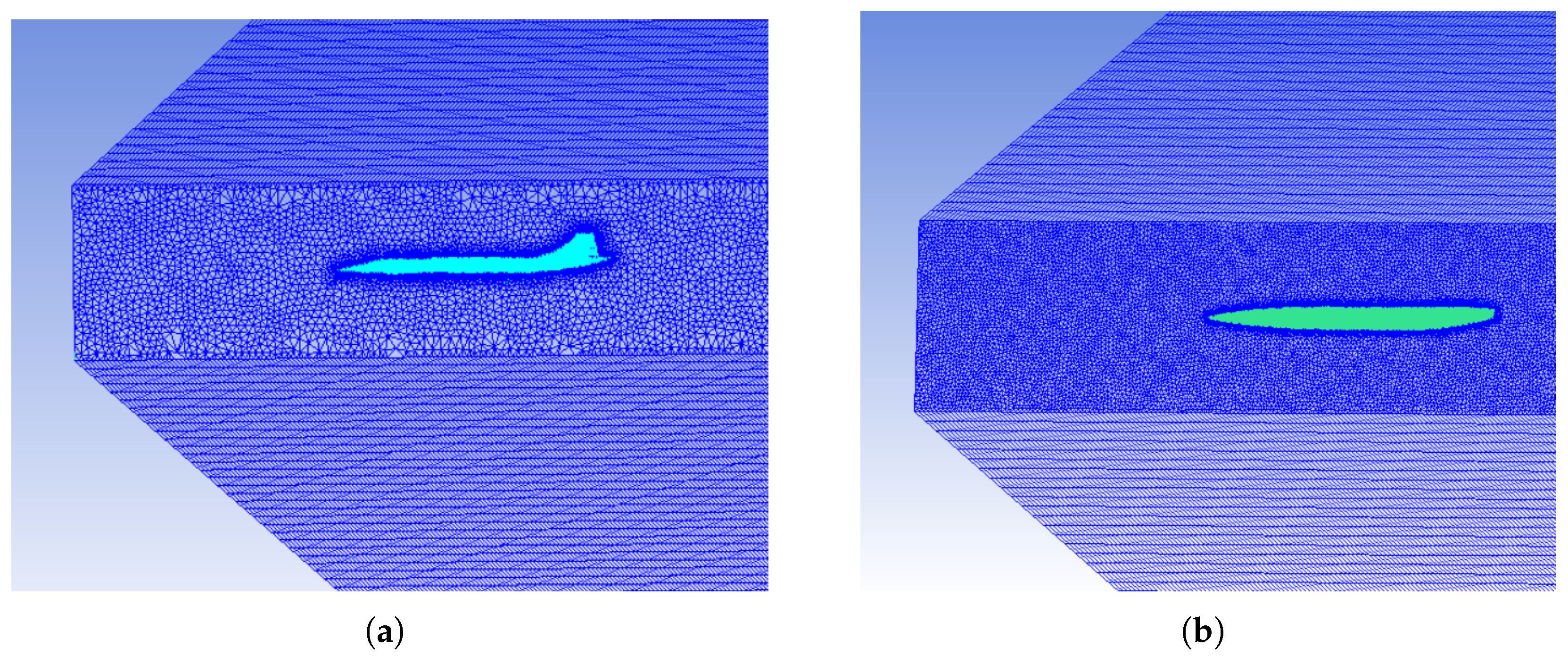
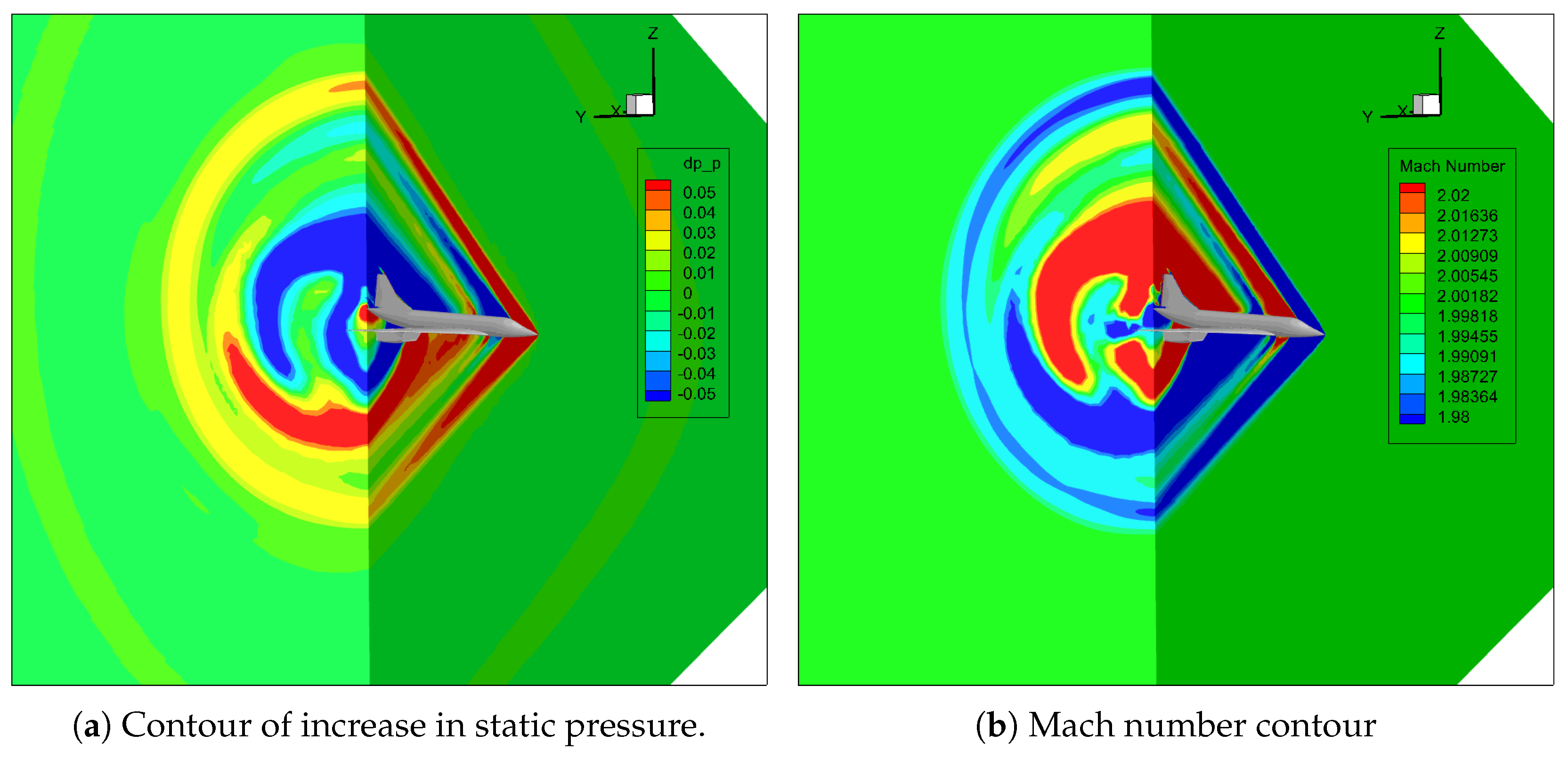
For the CS1 case study, the shock waves around the aircraft are clearly visible from the contours in Figure 11 which are obtained for a Mach 2 cruise speed and an angle of attack equal to 2°. The flow field below the aircraft is different from the flow field above the vehicle.

The pressure signature for the azimuth angle equal to 0° and the one in the 0–60° range is plotted in Figure 12: in particular, Figure 12a shows the on-track pressure signature and Figure 12b shows the radial pressure signature between 0° and 60°. The length of the sampled signal is about three aircraft lengths. In this way, the correct pressure signature in the near-field region can be evaluated and later propagated on the ground.

Figure 12b shows that peak pressure values decrease as the extraction lines shift from beneath the aircraft to the lateral regions near the wings. Additionally, the shape of the pressure signature varies significantly across different extractions, indicating changes in the interactions between shockwaves.

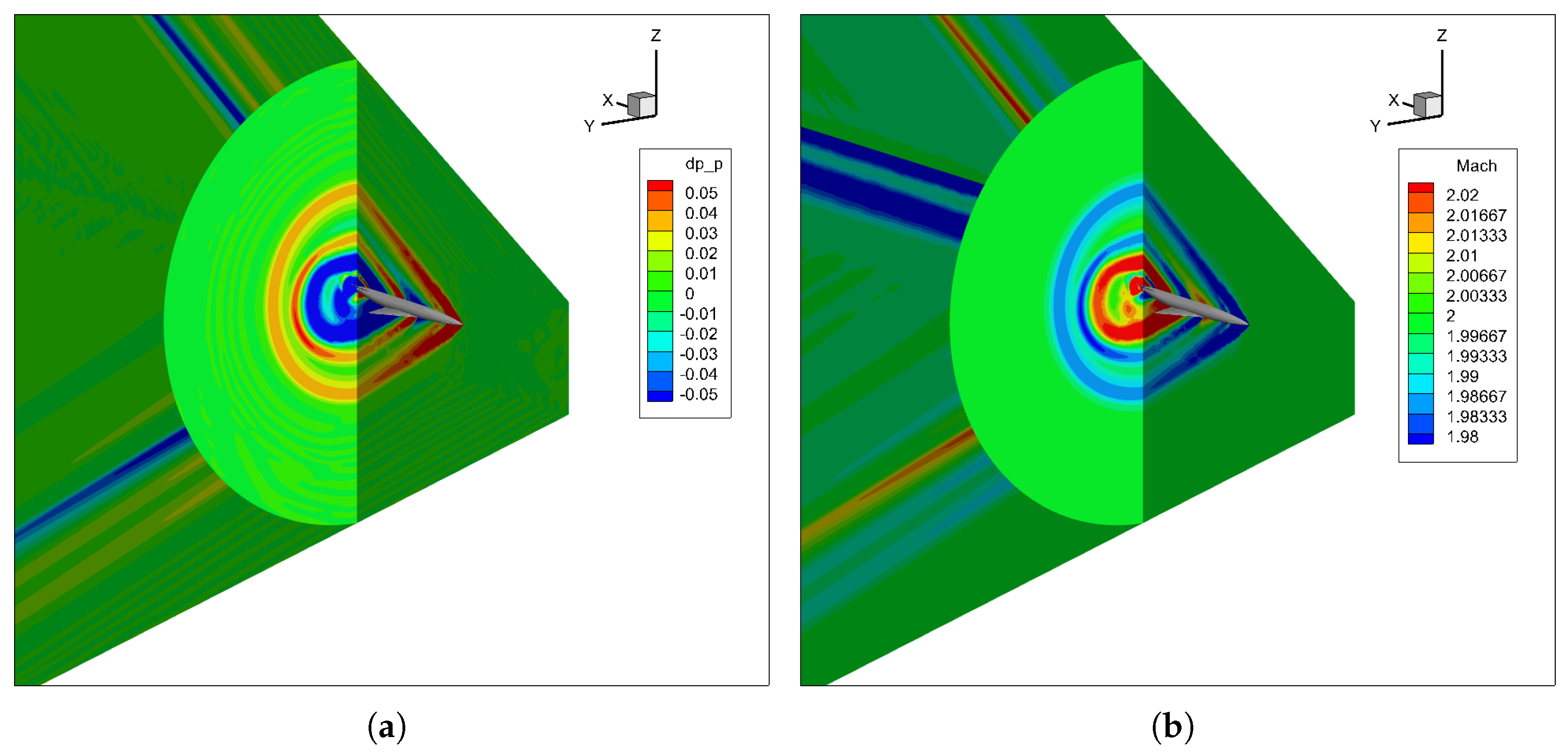
4.2. Near-Field Results—CS2

The same considerations were applied to the CS2 aircraft for different flight conditions. The simulated scenarios represent off-design conditions, with Mach numbers of 1.2 and 2.0, compared to the nominal cruise condition at Mach 5 and an altitude of 28 km.

As noticeable in Figure 13, the shock waves are clearly visible for this configuration.

As in the previous case, the pressure signature was extracted for both the on-track and off-track conditions for a range of angles between 0° and 60°, with the same 10° step, and it is visible in Figure 14.

It is possible to notice how the different shape of the aircraft as well as the angle of attack strongly influence both the on-track and off-track pressure signature: Figure 14a highlights the on-track pressure signature and Figure 14b highlights the off-track behaviour. As in the previous case, different extraction angles lead to a completely different shape of pressure signature, with strong differences in the expansion region.

4.3. Far-Field Results—CS1

To account for these effects of a non-uniform medium, far-field propagation is performed using the NASA-developed PCBoom solver, and the results previously obtained in Section 4.1 are used as input data.

In this paper, the analysis focuses solely on the pressure signatures observed on the ground, as this aligns with the primary aim of the study. Consequently, details regarding the width of the primary carpet are excluded from the discussion. Also, the loudness metrics results are not presented in this work since they are not input for the development of the low-fidelity method.

Some of the results of the propagated sonic boom waveforms on the ground for the CS1 are visible in Figure 15 for different angles of attack or atmospheres evaluated.

The pressure signature highlighted in Figure 15 are related to an observer placed with an azimuth angle equal to 0°, and at an ideal altitude of 5 m above ground level. The differences in the pressure signature for each configuration are purely given by the different Mach number and angle of attack.

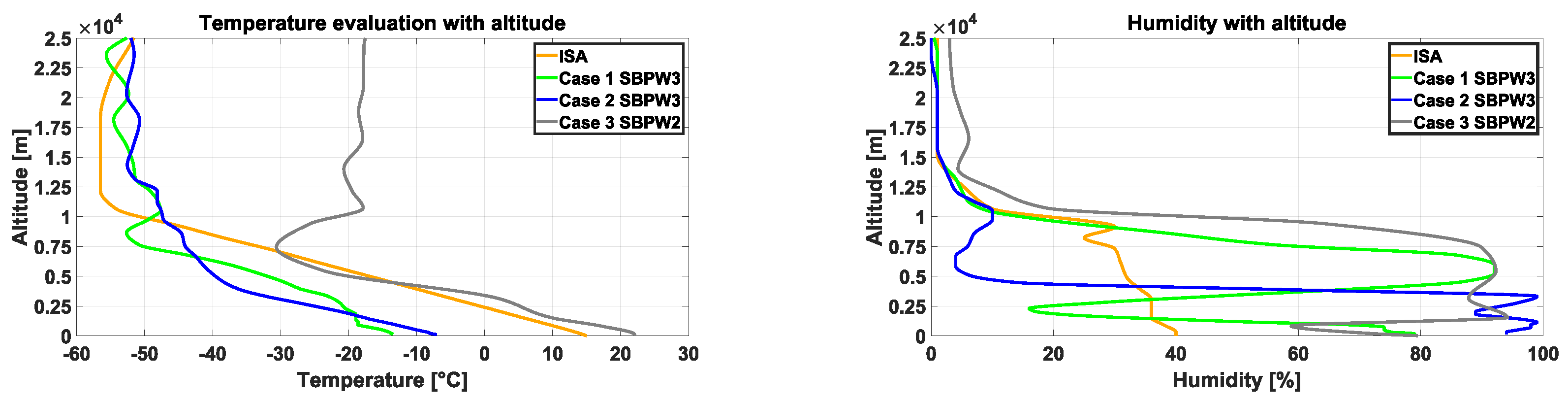
Figure 15 highlights the differences between different angles of attack in a range between −2° and 4° (Figure 15a), as well as the use of different atmospheres, such as the ISA or two measured atmospheric profiles (Figure 15b). It is possible to highlight important differences in the ground pressure signature due to different angles of attack: for angles of 0° and −2°, the waveform is not a fully developed N-wave, while the use of a different atmospheric profile has some changes in the peak pressure but not in the shape of the waveforms.

The value of peak overpressure for these waveforms on the ground creates a database that is the input for the development of the low-fidelity model.

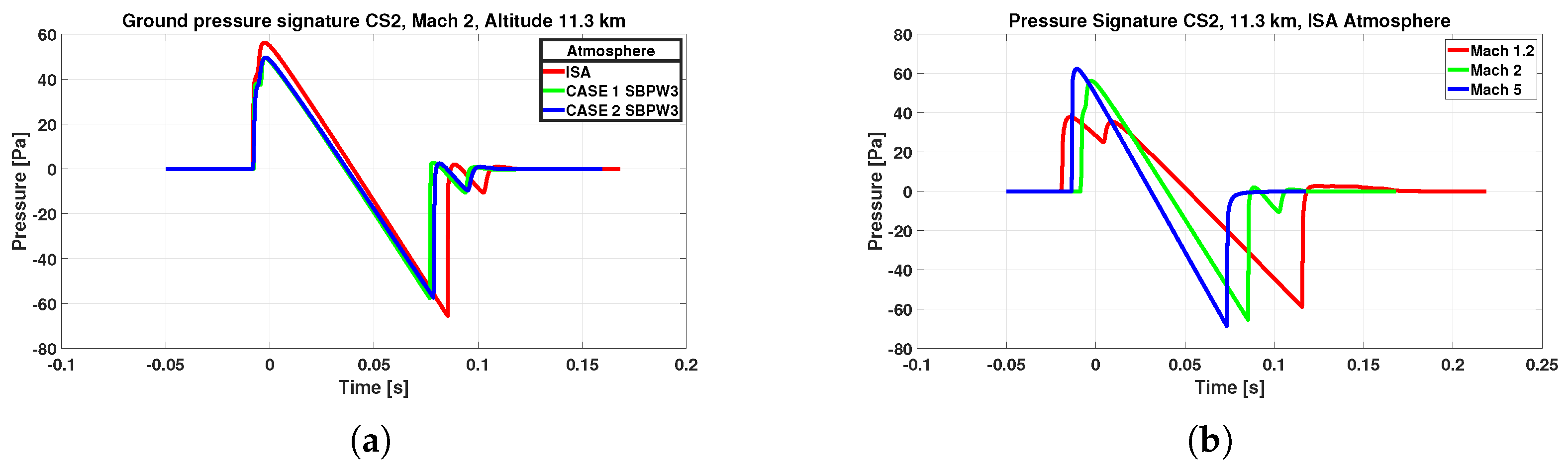
4.4. Far-Field Results—CS2

The previously adopted methodology has been applied to the CS2. In this case study, due to the particular angle of attack excursion during the mission profile, all simulations were conducted at an angle of attack of 0°. In Figure 16, it is possible to highlight the different sonic boom ground waveforms for different atmospheric profiles and Mach number.

In this work, just the two mission points at Mach 1.2 and Mach 2.0 were used in the development of the low-fidelity formulation. Figure 16a highlights the difference in the ground sonic boom waveforms due to different atmospheres, with some differences in the shape of the compression portion of the signature itself, while Figure 16b highlights the difference in the ground pressure signature due to different Mach numbers. The variation in the shape of the pressure signature is critically influenced by the Mach number, as can be seen in Figure 16b: higher Mach numbers cause higher peak pressure and shorter time signatures.

5. Sonic Boom Assessment: Low-Fidelity Results

In this context, now that high-fidelity results are available, the model performance was assessed, demonstrating its reliability and precision. A key indicator of the model’s success is the coefficient of determination $R^2$, which measures how well the predictions align with the observed data. In particular, the values obtained are 0.97 for the positive pressure peak $\Delta p_1$ and 0.93 for the negative pressure peak $\Delta p_2$, highlighting an optimal fit. This score validates the model’s accuracy and enhances confidence in its predictive power.

The model ability to generate accurate equations for $\Delta p_1$ and $\Delta p_2$ underscores its effectiveness. These equations provide critical insights into the system behaviour, and their precision is crucial for any further analysis or practical applications. The equations are as follows:

$$\Delta p_1=1.1149+0.2792·M-0.0537·h+0.1876·\alpha +6.764·{10}^{-4}·S$$

(7)

$$\Delta p_2=-1.8677-0.1046·M+0.0670·h-0.0579·\alpha -4.463·{10}^{-4}·S$$

(8)

In Equations (7) and (8), M is the Mach number [-], h is the altitude [km], $\alpha$ is the angle of attack [deg], and S is the wing area [m²]. Each explicit number represents a coefficient of the vectors $b_{1linear}$ and $b_{2linear}$, respectively.

The numerical values obtained by inserting the data related to supersonic cruise and the final wing surface of the case study are as follows:

• $\Delta p_1=47.75$ Pa
• $\Delta p_2=-49.66$ Pa

Coming back to the requirements specified in Section 2.2, the aircraft seems to satisfy both the maximum peak overpressure limit as well as the cumulative value of overpressure and expansion. To effectively integrate the evaluation of the requirement within the performance-oriented design space and address the gap discussed in Section 1 regarding the lack of environmental prescriptions for sonic boom in the design process, the equations mentioned must be reformulated to be a function of the wing loading. In this respect, Equation (7) is first reordered to explain the wing surface and then the wing loading is introduced by inverting and multiplying for the aircraft weight. This weight is expressed on one side as MTOW and on the other as W purely to highlight a notation attributable to the Matching Chart. Considering a single value, both represent the same. This adjustment ensures compatibility with the Matching Chart. Thus, a proper Matching Chart requirement for sonic boom is provided below, focusing solely on the overpressure peak.

Considering the conceptual design stage, peak pressure has been considered as a first indicator for assessing the potential annoyance induced by the sonic boom. While more sophisticated loudness-based metrics, such as perceived level (PLdB) or A-weighted sound exposure level (ASEL), would provide a more comprehensive assessment of human perception, the early stage of the design process necessitates a rapid evaluation approach.

The derived formulation, relating the wing loading to the requirement associated with the maximum overpressure peak, exploiting the correlation model presented in Section 5, can be expressed as follows:

$${\displaystyle \frac{W}{S}}={\displaystyle \frac{MTOW·6.764·{10}^{-4}}{\Delta p-(1.1149+0.2792·M-0.0537·h+0.1876·\alpha )}}$$

(9)

where the explicit coefficients are the ones obtained for $\Delta p_1$ in Equation (7). As it is written, this equation implies that the wing loading is exactly equal to the value for which a specific overpressure peak is obtained. Considering that the requirement states that the peak amplitude shall be strictly lower than the prescribed value, wing loading for the aircraft under study shall be higher than the value resulting from the right side of the equation. This will impose a new limit to the left side of the x-axis in the Matching Chart, which was not previously present, introducing an additional boundary, in parallel to the maximum wing loading representing the landing or stall condition.

The derivation of the aforementioned boundary allows defining an updated Matching Chart that is visible in Figure 17.

The current vehicle configuration already satisfies the sonic boom requirement, since the wing loading prescribed by performance requirements to minimize the required thrust is already higher than the left limit specified by the sonic boom requirement.

However, the possibility of introducing a lower limit on wing loading on the left side of the Matching Chart becomes crucial for specific aircraft configurations that may fall into areas of the design space previously considered feasible but which, in light of new environmental constraints, prove to be unacceptable. By incorporating the sonic boom requirement, the Matching Chart evolves into a more comprehensive tool that not only evaluates aerodynamic and performance characteristics but also ensures early compliance with emerging environmental regulations.

This added constraint enhances the designer’s ability to identify trade-offs between thrust, wing area, and noise impact from the very beginning of the conceptual design process. As such, it supports a more informed and environmentally conscious approach to the sizing and selection of the baseline configuration. This lays the groundwork for more advanced optimization processes, particularly in view of future noise regulations for overland supersonic flight.

6. Conclusions

This study presents a novel methodology for incorporating sonic boom constraints directly into the Matching Chart, a fundamental tool in conceptual aircraft design. By leveraging a hybrid multi-fidelity approach based on high-fidelity CFD simulations and propagation models—as well as a low-fidelity statistical regression model—the peak ground-level overpressure generated by supersonic flight can be estimated efficiently and accurately.

The results clearly indicate that sonic boom constraints can and should be included from the earliest stages of aircraft development. The integration of this constraint into the Matching Chart enables designers to visualize and respect environmental limitations while evaluating aerodynamic and performance trade-offs. The newly introduced boundary linked to overpressure limits enhances the traditional design space by explicitly accounting for community noise impact, a key factor for the viability of future supersonic transports.

The proposed methodology has been demonstrated on a representative Mach 1.5, 80-passenger aircraft configuration, showing compliance with both performance and sonic boom requirements. Notably, the current design satisfies the sonic boom constraint without sacrificing performance, but the introduction of the new requirement has the potential to significantly influence future design iterations and concept evaluations.

Future work will aim to generalize and refine the sonic boom formulation for broader applicability across different aircraft categories and mission profiles. Additionally, the incorporation of more advanced acoustic metrics—such as perceived loudness level (PLdB)—and the analysis of airport-related noise (e.g., LTO cycles) will further strengthen the environmental integration within the design process. Ultimately, the methodology could be embedded in a fully multidisciplinary optimization loop, enabling seamless trade-offs between aerodynamics, propulsion, structure, and acoustics in support of next-generation sustainable supersonic aviation.