Numerical Investigation of Tar Formation Mechanisms in Biomass Pyrolysis

Abstract

This study achieves the particle-resolved modeling of biomass pyrolysis via a novel approach of integrating the Discrete Element Method (DEM) with a semi-detailed chemical kinetic mechanism. By coupling CFD-DEM with a 36-step reaction network, the multiscale interactions between particle-scale hydrodynamics and the formation kinetics of 19 tar components under varying temperatures (630–770 °C) are elucidated. Levoglucosan (44.79%) and methanol (18.64%) are identified as primary tar components. Combined with these, furfural (C₅H₄O₂, 7.22%), methanal (CH₂O, 6.75%), and glutaric acid (C₅H₈O₄, 4.20%) account for over 80% of all the tar components. The secondary decomposition pathways are successfully captured, and changes in the reaction rates, as seen in triglycerides (R23: 307.30% rate increase at 770 °C) and tannins (R24: 265.41% acceleration), are quantified. This work provides the ability to predict intermediate products, offering critical insights into reactor optimization.

1. Introduction

The International Civil Aviation Organization’s 2050 net-zero emissions mandate underscores the urgency of sustainable aviation fuel (SAF) development. The American Society of Testing Materials (ASTM) has approved 11 SAF synthesis technology routes, with the most mature being the Hydrotreated Esters and Fatty Acids (HEFAs) route that employs used cooking oil (UCO) as a raw material. However, it is limited by its high cost. The Fischer–Tropsch (FT) route, using biomass as a raw material, has a significant price advantage. While biomass-derived SAF presents a carbon-negative pathway through high-temperature pyrolysis, tar formation during pyrolysis and gasification remains a critical bottleneck, causing equipment corrosion and operational inefficiencies and restricting the promotion of SAF [1,2]. The harmfulness of tar has been recognized, and mechanisms of tar formation during biomass pyrolysis have also been studied gradually [3,4,5,6]. The current experimental approaches face challenges in the real-time analysis of tar components, whereas numerical simulations enable cost-effective reactor optimization by capturing the spatial distributions of intermediates and reaction intensities—parameters often experimentally inaccessible. Therefore, numerical simulation is beneficial for scaling production technologies.

Proposed by Cundall and Strack in 1980 [7], the Discrete Element Method (DEM) solves individual particle motion, collision, and chemical reactions. While DEM offers higher particle-level accuracy than Multiphase-Particle In Cell (MP-PIC) [8], its computational demand has historically limited its applications. Meanwhile, recent advancements in hardware and parallel algorithms have expanded the utility of DEM. For instance, Oevermann et al. [9] applied the DEM to simulate wooden char gasification in fluidized beds. Therein, the particle reaction used a shrinking core model, the collision between particles was simulated using the DEM method, the gas phase turbulence was simulated using large eddy simulation, and the Smagorinsky model acted as a subgrid model. Considering the mass and heat transfer between gas–solid phases, the single particle pyrolysis and gasification process were studied. Ku et al. used the CFD-DEM method to simulate a quasi-two-dimensional biomass fluidized bed [10]. Pine wood was used as biomass particles, the fluidized gas was nitrogen, and the gasifying agent was water. The experimental results were consistent with those in another study [11], wherein the effects of the particle injection location, reactor temperature, and steam/biomass mass ratio on gasification were investigated, and so were the differences in flow patterns between dry and wet particles [12] and the thermodynamic thickness of particles [13].

Biomass pyrolysis involves complex interactions among heterogeneous components (cellulose, hemicellulose, lignin) and multiphase reactions [14]. Currently, the most common pyrolysis reaction model used is the single-step model. Although it offers good computational efficiency, it lacks universality because it cannot reflect the impact of changes in the composition of raw materials. In addition, it cannot predict the intermediate products during the pyrolysis process, such as tar components, which are harmful to facilities and difficult to measure online in experiments. Obviously, the more detailed the reaction model is, the better the simulation results, whereas this will bring about a huge amount of computation that is difficult to achieve. As a compromise, semi-detailed mechanisms balance accuracy and complexity. On the basis of the Broido–Shafizadeh (B-S) reaction mechanism model proposed by Broido and Shafizadeh et al. [15,16], Ranzi et al. presented a semi-detailed model in 2008, which combines the individual pyrolysis mechanisms of cellulose, hemicellulose, and lignin. This model includes the second-order gas-phase pyrolysis reactions of some important pyrolysis products [17,18,19,20,21].

To simulate biomass pyrolysis, this study employs the DEM method based on the Euler–Lagrange framework, coupled with a modified, semi-detailed chemical mechanism. Addressing the gaps between particle-scale phenomena and system-level performance, tar formation, intermediate product distributions, reaction intensities, and particle dynamics are analyzed.

2. Methodology

2.1. Hydrodynamic Modeling

The numerical simulations in this study consider gas–solid two-phase flow, heat and mass transfer, and chemical reactions. The CFD-DEM framework incorporates gas–solid flow (Equations (1)–(9)), heat transfer (Equations (10)–(21)), and shrinking core particle dynamics (Equation (22)). The key assumptions are as follows: (1) no pressure or temperature gradients exist within the particles; (2) the water–gas shift reaction is in equilibrium; (3) gas reactant transport occurs solely through diffusion, (4) particles are spherical, (5) the gas inside the particles is quasi-steady, and (6) the particle radius decreases continuously as pyrolysis proceeds. The mathematical model is explained below.

A.

Governing equation.

The continuity equation of fluid phase is presented in Equation (1):

$${\displaystyle \frac{\partial \left({\epsilon }_g{\rho }_g\right)}{\partial t}}+\nabla ·\left({\epsilon }_g{\rho }_g{\mathit{u}}_{\mathit{g}}\right)=\delta \dot{m_p}$$

(1)

The fluid phase momentum equation is presented in Equation (2):

$${\displaystyle \frac{\partial \left({\epsilon }_g{\rho }_g{\mathit{u}}_{\mathit{g}}\right)}{\partial t}}+\nabla ·\left({\epsilon }_g{\rho }_g{\mathit{u}}_{\mathit{g}}{\mathit{u}}_{\mathit{g}}\right)=\nabla ·\left({\epsilon }_g{\mathit{\tau }}_{\mathit{g}}\right)-\nabla \mathrm{p}+{\epsilon }_g{\rho }_{g}g-{\displaystyle \sum }_{m=1}^M{I}_{gm}$$

(2)

The stress tensor is presented in Equation (3):

$${\tau }_{gij}={\mu }_g\left({\displaystyle \frac{\partial u_{gi}}{\partial x_j}}+{\displaystyle \frac{\partial u_{gj}}{\partial x_i}}\right)-{\displaystyle \frac{2}{3}}{\mu }_g{\displaystyle \frac{\partial u_{gk}}{\partial u_{gk}}}{\delta }_{ij}$$

(3)

where $I_{gm}$ represents the momentum exchange term between the gas phase and the solid phase (sand or biomass), and ${\delta }_{ij}$ denotes the Kronecker triangle.

In the Lagrangian method, particle motion is calculated by Newton’s second law, which is presented in Equations (4) and (5):

$$m_p{\displaystyle \frac{d{\mathit{u}}_{\mathit{p}}}{dt}}={\mathit{F}}_{\mathit{d}}-V_p\nabla p+m_p\mathit{g}+{\mathit{F}}_{\mathit{c}}$$

(4)

$$I_p{\displaystyle \frac{d\mathit{\omega }}{dt}}=\mathit{T}$$

(5)

where $m_p$ denotes the particle mass, ${\mathit{u}}_{\mathit{p}}$ denotes the particle velocity, $V_p$ denotes the particle volume, $I_p$ denotes the particle’s moment of inertia, ω denotes the particle’s angular velocity, and T is the particle’s torque. On the right-hand side of the equation, the first term, ${\mathit{F}}_{\mathit{d}}$, represents drag force, which is the interaction force between the particle and the surrounding fluid. At present, the drag force is calculated through a semi empirical relationship, which will be discussed in detail later. The second term comes from the pressure difference around the particles, the third term comes from gravity, and the fourth term, ${\mathit{F}}_{\mathit{c}}$, is the indirect contact force between solids, including particles and walls.

B.

Contact force model.

This study uses the Linear Spring Dashpot (LSD) model as the contact force model, which treats the particle as a small ball with elasticity. The collision of elastic balls is processed into the motion of a spring damping slider system. Therefore, the contact force is considered as the sum of spring force, damping force, and friction force.

C.

The drag model is presented in Equations (6)–(9):

$${\mathit{F}}_{\mathit{d}}={\displaystyle \frac{V_p\beta }{{\epsilon }_p}}\left({\mathit{u}}_{\mathit{f}}-{\mathit{u}}_{\mathit{p}}\right)$$

(6)

$$\beta =\{\begin{array}{c}150{\displaystyle \frac{{\epsilon }_p^2{\mu }_f}{{\epsilon }_f^2{d}_p^2}}+1.75{\displaystyle \frac{{\epsilon }_p{\rho }_f}{{\epsilon }_f{d}_p}}\left|{\mathit{u}}_{\mathit{f}}-{\mathit{u}}_{\mathit{p}}\right| {\epsilon }_f<0.8\\ {\displaystyle \frac{3}{4}}{C}_d{\displaystyle \frac{{\epsilon }_p{\rho }_f}{d_p}}\left|{\mathit{u}}_{\mathit{f}}-{\mathit{u}}_{\mathit{p}}\right|{\epsilon }_f^{-2.65} {\epsilon }_f\ge 0.8\end{array}$$

(7)

$$C_d=\{\begin{array}{c}{\displaystyle \frac{24}{R{e}_p}}\left(1+0.15R{e}_p^{0.687}\right) R{e}_p<1000\\ 0.44 R{e}_p\ge 1000\end{array}$$

(8)

$$R{e}_p={\displaystyle \frac{{\epsilon }_f{\rho }_f{d}_p\left|{\mathit{u}}_{\mathit{f}}-{\mathit{u}}_{\mathit{p}}\right|}{{\mu }_f}}$$

(9)

where β represents the momentum exchange coefficient between phases, which is given according to a semi-empirical relationship. This article adopts the Gidaspow relationship, which is commonly used for simulating fluidized beds.

E.

Heat and mass transfer equation.

The gas-phase mass transfer equation is presented in Equation (10):

$$\frac{\mathrm{\partial }\left({\epsilon }_g{\rho }_f{Y}_{f,i}\right)}{\mathrm{\partial }t}+\mathrm{\nabla }\cdot \left({\epsilon }_g{\rho }_g{Y}_f{\mathit{u}}_f\right)=\mathrm{\nabla }\cdot \left(D_i{\epsilon }_g{Y}_{f,i}\right)+\delta {\dot{m}}_{i,chem}$$

(10)

The conservation equation of internal energy in the gas phase is presented in Equation (11):

$${\epsilon }_g{\rho }_g{C}_{pg}\left({\displaystyle \frac{\partial T_g}{\partial t}}+u_{gj}{\displaystyle \frac{\partial T_g}{\partial x_j}}\right)=-{\displaystyle \frac{\partial }{\partial x_i}}\left(-k_g{\displaystyle \frac{\partial T_g}{\partial x_i}}\right)+q_{gs}-\Delta H_{rg}+{\gamma }_{Rg}\left(T_{Rg}^4-T_g^4\right)$$

(11)

The first term on the right-hand side represents thermal conductivity, the second term represents heat transfer between gas and solid, the third term represents chemical heat, and the last term represents gas-phase radiative heat transfer, where ${\gamma }_{Rg}$ represents the gas-phase radiative heat transfer coefficient, and $T_{Rg}$ represents the gas-phase radiative temperature.

The conservation of internal energy of particles is presented in Equation (12):

$$m_p{C}_{p,p}{\displaystyle \frac{d{T}_p}{dt}}={\dot{Q}}_{pp}+{\dot{Q}}_{pfp}+{\dot{Q}}_{pg}+{\dot{Q}}_{rad}-\Delta H_{rs}$$

(12)

where $T_p$ denotes the particle temperature, and $C_{p,p}$ is the specific heat of the particle. On the right-hand side, ${\dot{Q}}_{pp}$ represents the heat conduction between particles, ${\dot{Q}}_{pfp}$ represents the heat conduction between particles–fluid–particles, ${\dot{Q}}_{pg}$ represents the convective heat transfer between particles and gas, and ${\dot{Q}}_{rad}$ represents the radiative heat transfer between particles. $\Delta H_{rs}$ is the heat of the chemical reaction.

The heat conduction between particles is given by Batchelor and O’Brien’s model, presented in Equation (13):

$${\dot{Q}}_{pp}^{ij}={\displaystyle \frac{4k_p^i{k}_p^j}{k_p^i+k_p^j}}\sqrt{{R_p^k}^2-{\left({\displaystyle \frac{{R_p^k}^2-{R_p^l}^2+l_{ij}^2}{2l_{ij}}}\right)}^2}\left(T_p^j-T_p^i\right)$$

(13)

where $k_p$ represents the thermal conductivity; the subscripts i and j, respectively, represent the numbers of the two particles in contact; $R_p$ is the radius of the particle; and $l_{ij}$ is the distance between the centers of particles.

The particle–fluid–particle thermal conductivity is given according to Rong and Horio’s formula, presented in Equation (14):

$${\dot{Q}}_{pfp}^{ij}=k_g\left(T_p^j-T_p^i\right){{\displaystyle \int }}_{R_c}^{R_f}{\displaystyle \frac{2\pi r}{l^{ij}-\left({\left(R_p^i-r^2\right)}^{\frac{1}{2}}+{\left(R_p^j-r^2\right)}^{\frac{1}{2}}\right)}}dr$$

(14)

where

$$R_c=\{\begin{array}{c}0 l^{ij}>2R_p \\ \sqrt{{R_p^k}^2-{\left({\displaystyle \frac{{R_p^k}^2-{R_p^l}^2+l_{ij}^2}{2l^{ij}}}\right)}^2} l^{ij}\le 2R_p\end{array}$$

(15)

$$R_p^k=max\left\{R_p^i,R_p^j\right\}$$

(16)

$$R_p^l=min\left\{R_p^i,R_p^j\right\}$$

(17)

where $R_f$ denotes the upper boundary of the range of particle–fluid–particle thermal conductivity, and $R_c$ is the radius of the circle formed by the contact area between two spheres.

The convective heat transfer between particles and gases is presented in Equation (18):

$${\dot{Q}}_{pg}={\gamma }_{cp}{A}_s\left(T_g-T_p\right)$$

(18)

The convective heat transfer coefficient, $h_{pf}$, is calculated according to the Ranz–Marshall relationship, which is presented in Equation (19):

$$N{u}_{fp}={\displaystyle \frac{{\gamma }_{fp}}{k_g/2R_p}}=2+0.6R{e}^{0.5}P{r}^{0.33}$$

(19)

The radiation between particles is presented in Equations (20) and (21):

$${\dot{Q}}_{rad}^i={ϵ}_{rad}{A}_s^i\sigma \left(T_{env}^4-T_i^4\right)$$

(20)

$$T_{env}={\displaystyle \frac{1}{N_{p,\Omega }}}{\displaystyle \sum }_{j=1,j\ne i}^{N_{p\Omega }}{T}_p^j$$

(21)

where ${ϵ}_{rad}$ denotes emissivity; $T_{env}$ denotes the ambient temperature of the surrounding particles, which is the average temperature of all particles within the neighborhood Ω; and $N_{p\Omega }$ is the number of particles in the neighborhood.

E.

Shrinking core model

In the shrinking core model, it is assumed that the density within particles is uniform, and all the mass lost in the reaction is reflected in the particle diameter reduction. This model is simple, reliable, and robust; hence, it is widely used in most similar simulations. It serves as a basis for the rate formula of the solid-phase reaction equation; therefore, this model is compatible with models related to solid-state reactions, which is presented in Equation (22):

$$d_p=\sqrt[3]{{\displaystyle \frac{6m_p}{\pi \rho }}}$$

(22)

2.2. Semi-Detailed Chemical Mechanism

The semi-detailed chemical mechanism used in this article is mainly based on the pyrolysis reaction model developed by Ranzi et al. [17,20] and combined with the research of Debiagi et al. [22], Lu et al. [23], and Li et al. [8] It has been modified to adapt the scenario of this article, including drying, pyrolysis, and gasification. The detailed reactions are listed in

Table 1. Semi-detailed chemical mechanism.

No.	Chemical Equation	k (1/s)	E (Cal/mol)
1	CO + H2O↔CO2 + H2	Ref. [4]
2	CH4 + H2O→CO + 3*H2	Ref. [4]
3	Char + CO2→2*CO	Ref. [4]
4	Char + H2O→CO + H2	Ref. [4]
5	Cellulose→Active Cellulose	1.50 × 1014	4.70 × 104
6	Active Cellulose→0.05*CH2OHCH2CHO + 0.4*CH2OHCHO + 0.03*CHOCHO + 0.17*CH3CHO + 0.25*C6H6O3 + 0.35*C2H5CHO + 0.2*CH3OH + 0.15*CH2O + 0.49*CO + 0.43*CO2 + 0.13*H2 + 0.93*H2O + 0.02*HCOOH + 0.05*CH4 + 0.66*CHAR + 0.05*G_CO + 0.05*G_CO_H2_L + 0.1*G_H2	2.50 × 106	1.91 × 104
7	Active Cellulose→C6H10O5	3.30 × T	1.00 × 104
8	Cellulose→0.125*H2 + 4.45*H2O + 5.45*CHAR + 0.12*G_CO_H2_S + 0.25*G_CO + 0.18*G_CO_H2_L + 0.125*G_H2	9.00 × 107	3.10 × 104
9	GMSW_C5H8O4→0.7*HCE1_C5H8O4 + 0.3*HCE2_C5H8O4	1.00 × 1010	3.10 × 104
10	XYHW_C5H8O4→0.35*HCE1_C5H8O4 + 0.65*HCE2_C5H8O4	1.25 × 1011	3.14 × 104
11	XYGR_C5H8O4→0.12*HCE1_C5H8O4 + 0.88*HCE2_C5H8O4	1.25 × 1011	3.00 × 104
12	HCE1_C5H8O4→0.06*CH2OHCH2CHO + 0.16*FURFURAL_C5H4O2 + 0.1*CHOCHO + 0.13*C6H6O3 + 0.09*CO2 + 0.02*H2 + 0.1*CHAR + 0.54*H2O + 0.25*C6H10O5 + 0.1*CH4 + 0.25*C5H8O4	16.0 × T	1.29 × 104
13	HCE1_C5H8O4→0.4*CH2O + 0.49*CO + 0.39*CO2 + 0.1*H2 + 0.4*H2O + 0.975*CHAR + 0.05*HCOOH + 0.175*C2H4 + 0.625*CH4 + 0.37*G_CO_H2_S + 0.51*G_CO2 + 0.01*G_CO + 0.43*G_CO_H2_L + 0.05*G_H2 + 0.2*G_C2H6	3.0 × 10−3 × T	3.60 × 103
14	HCE2_C5H8O4→0.145*FURFURAL_C5H4O2 + 0.105*CH3CO2H + 0.035*CH2OHCHO + 0.3*CO + 0.5125* CO2 + 0.5505* H2 + 0.056* H2O + 0.2395*CH4 + 0.0175*HCOOH + 0.049*C2H5OH + 0.7125*CHAR + 0.45*G_CO2 + 0.78*G_CO_H2_S + 0.105*G_CH3OH + 0.1*C2H4 + 0.18* G_CO_H2_L + 0.21*G_H2 + 0.2*G_C2H6	7.0 × 109	3.05 × 104
15	LIGH_C22H28O9→0.2*CH2OHCHO + 0.5*C2H5CHO + 0.1*CO + 0.4*C2H4 + 0.1*C2H6 + LIGOH_C19H22O8	6.70 × 1012	3.75 × 104
16	LIGO_C20H22O10→CO2 + LIGOH-C19H22O8	3.30 × 108	2.55 × 104
17	LIGC_C15H14O4→0.1*C6H5OCH3 +0.22*CH2O +0.21*CO + 0.1*CO2 +0.27*C2H4+ 0.2*G_C2H6 + 0.1*VANILLIN_C8H8O3 + 0.35*LIGCC_C15H14O4 + 5.85*CHAR + 0.4*G_CO_H2_S + 0.36*CH4 + 0.17*G_CO_H2_L + H2O + 0.1*G_H2	1.00 × 1011	3.72 × 104
18	LIGCC_C15H14O4→0.15*C6H5OCH3 +0.35* CH2OHCHO + 1.15*CO +0.7*H2 + 0.7*H2O + 0.45*CH4 + 0.25*VANILLIN_C8H8O3 + 0.15*CRESOL_C7H8O + 0.4*C2H6 + 6.8*CHAR + 0.3*C2H4 + 0.4*G_CO	1.00 × 104	2.48 × 104
19	LIGOH-C19H22O8→0.025*C24H28O4 + 0.1*C2H3CHO + 0.6*CH3OH + 0.65*CO + 0.6*G_CO + H2O + 0.05*HCOOH + 0.35*CH4 + 4.25*CHAR + 0.05*CO2 + 0.9*LIG_C11H12O4 + 0.1*C2H4 + 0.45*G_CO_H2_L + 0.3*G_CH3OH + 0.15*G_C2H6 + 0.4*G_CO_H2_S	1.50 × 108	3.00 × 104
20	LIG_C11H12O4→0.1*C6H5OCH3 + 0.3*CH3CHO + 0.6*CO + 0.5*C2H4 + VANILLIN_C8H8O3 + 0.1*CHAR	4.00 × T	1.20 × 104
21	LIG_C11H12O4→0.4*CH2O + 0.3*CO + 0.6*H2O + 0.6*CH4 + 6.1*CHAR + 0.1*CO2 + 0.65*G_CO_H2_S + 0.2*G_CO + 0.4*G_CH3OH + 0.5*C2H4 + 1.25* G_CO_H2_L + 0.1*G_H2	0.083 × T	0.80 × 104
22	LIG_C11H12O4→0.4*CH3OH + 0.4*CH2O + 2.6*CO + 0.6*H2O + 0.75* C2H4 + 0.6*CH4 + 0.5*C2H6 + 4.5*CHAR	1.50 × 109	3.15 × 104
23	TGL_C57H10O7→C2H3CHO + 0.5*C13H22O2 + 2.5*C19H34O2	7.00 × 1012	4.57 × 104
24	TANN_C15H12O7→H20 + 0.85*C6H5OH + ITANN_C8H4O4 + G_CO + 0.15*G_C6H5OH	2.00 × 101	1.00 × 104
25	ITANN_C8H4O4→2*CO + H2O + 5*CHAR + 0.45*G_CO_H2_S + 0.55*G_CO_H2_L	1.00 × 103	2.50 × 104
26	G_CO2→CO2	1.00 × 10⁶	2.45 × 104
27	G_CO→CO	5.00 × 1012	5.25 × 104
28	G_CH3OH→CH3OH	2.00 × 1012	5.00 × 104
29	G_CO_H2_L→0.2*CO + 0.2*H2 + 0.8*H2O + 0.8*CHAR	6.00 × 1010	5.00 × 104
30	G_C2H6→C2H6	1.00 × 1011	5.20 × 104
31	G_CH4→CH4	1.00 × 1011	5.30 × 104
32	G_C2H4→C2H4	1.00 × 1011	5.40 × 104
33	G_C6H5OH→C6H5OH	1.50 × 1012	5.50 × 104
34	G_CO_H2_S→0.8*CO + 0.8*H2 + 0.2*H2O + 0.2*CHAR	1.00 × 109	5.90 × 104
35	G_H2→H2	1.00 × 108	7.00 × 104
36	MOISTURE→H2O	T	0.80 × 104

.

The thermal properties were mainly acquired from Alexander Burcat’s public thermodynamic data, and chemical formulas were labeled in their distinguished names. For simplicity, only tar components related to this article are listed in

Table 2. Thermal properties of tar components.

No.	Distinguished Name	Substance	Molecular Weight	Hf/R
1	CH2O	Methanal	28.0538	6314.2627
2	C2H3CHO	Acrolein	56.0642	−7941.6205
3	C2H5CHO	Propionaldehyde	58.0800	−22,268.8471
4	C2H5OH	Ethanol	46.0690	−28,257.8290
5	C5H8O4	Glutaric acid	132.1161	−76,265.7276
6	C6H10O5	Levoglucosan	162.1424	−101,107.1970
7	C6H5OCH3	Anisole	108.1399	−8605.9386
8	C6H5OH	Phenol	94.1130	−11,594.1217
9	C6H6O3	Pyrogallol	126.1118	−40,161.0469
10	C24H28O4	Aromatic dimer	380.4839	−123.721175
11	CH2OHCH2CHO	3-hydroxypropanal	74.07944	−40,412.6826
12	CH2OHCHO	Ethanol aldehyde	60.05256	−36,869.6787
13	CH3CHO	Acetaldehyde	44.05316	−19,987.9484
14	CH3CO2H	Acetic acid	60.05256	−51,987.3138
15	CH3OH	Methanol	32.04216	−24,174.6056
16	CHOCHO	Glyoxal	58.03668	−25,507.4563
17	CRESOL_C7H8O	Cresol	108.1399	−15,485.6569
18	FURFURAL_C5H4O2	Furfural	96.08556	−18,188.2234
19	VANILLIN_C8H8O3	Vanillin	152.1497	−44,656.4291

, where H_f stands for the standard enthalpy of formation, and R is gas constant.

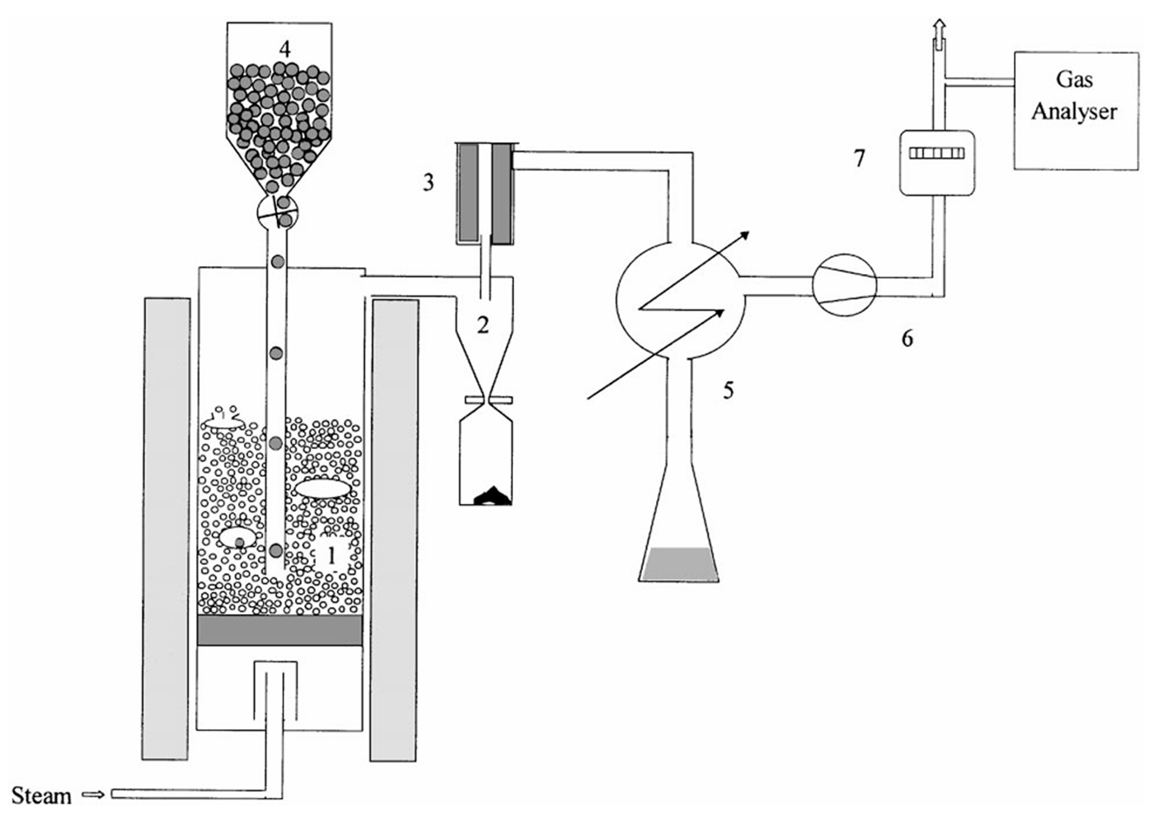
2.3. Case Description

The simulation setup employs nitrogen as the fluidizing gas, steam as the gasifying agent, and almond shell as the biomass feedstock. The gas composition comprises 80% nitrogen and 20% steam. As for the boundary conditions, a steam-to-biomass mass ratio of 1, a biomass feed rate of 300 g/h, and the inlet temperature of the gas are given. The pressure outlet condition is 1 atm at the top of the computational domain. As for the initial conditions, the fluidized bed has an inner diameter of 60 mm and an initial bed height of 132.6 mm, and the volume fraction of densely packed particles is 0.41. Sand particles (6852 total, 1 mm diameter, 2640 kg/m³ density) and biomass particles (1100 μm diameter, 1200 kg/m³ density) were set at the initial temperature. Simulations were conducted at 3 temperature levels: 630 °C, 700 °C, and 770 °C.

To balance the computational efficiency and resolution, a quasi-3D mesh with a thickness equal to the largest particle diameter (1.1 mm) and 1800 total cells (12 × 150 × 1) was used (Figure 1). Of note, a quasi-3D mesh is a common and reasonable simplification, though it causes potential differences in capturing complex flow structures or the non-uniformity of particle distribution within the reactor.

2.4. Experimental Validation

The experiments were carried out in the research of Rapagna [24]; hence, only a brief description is given here. The equipment consists of a bubbling fluidized-bed gasifier with a continuous biomass feeding system, gas cleaning section, cooling system for the separation of water and tar, and measurement devices. A schematic description is presented in Figure 2. The amount of the organic material condensed together with water is determined by means of a total carbon (TC) analysis being performed on samples taken every 10–30 min. The instantaneous and average values of the tar content of the gas stream at the exit of the gasifier are calculated assuming naphthalene as the representative tar compound. The quantity of dry gas produced is measured by means of a volumetric gas-meter. The concentrations of dry gas are monitored continuously using an infrared analyzer for CO, CO₂, and CH₄ and a thermal conductivity detector for H₂. The fluidizing medium is steam and the bed inventory is sand. The biomass comprises small round particles of crushed almond shells, and the feed rate is fixed at 0.3 kg/h. The experimental tests were carried out at 770 °C.

The DEM algorithm was first validated using a single-step pyrolysis mechanism [8]. As shown in

Table 3. Comparison between simulations and experiments.

Product		Experiment	DEM (Single-Step)	DEM (Semi-Detailed)
Gas	CO (Vol%)	33.2	32.9	24.8
	CO2 (Vol%)	11.7	12.9	21.0
	H2 (Vol%)	43.6	43.2	45.0
	CH4 (Vol%)	11.5	11.0	9.2
	LHV of the gas (kJ/Nm3)	13,018	12,764	10,873
Tar (g/Nm3)		43	—	116
Char (g/kg)		102	—	75.4

, the gas composition predictions (CO, CO₂, H₂, CH₄) align closely with the experimental data, proving that the established DEM algorithm has high accuracy.

However, adopting a semi-detailed mechanism increases discrepancies in CO and CO₂, attributed to model complexity. The calculated value of char production is 75.4 g/Nm³, while the experimental value is 102 g/Nm³, with a relative error of about 24%. The calculated value of tar production is 116.0 g/Nm³, while the experimental value is 43 g/Nm³, with a relatively large relative error of 170%. These errors are mainly caused by the semi-detailed pyrolysis mechanism model. First, the semi-detailed mechanism depends on a large amount of data, such as the pyrolysis reaction coefficient, reaction heat, and reaction rate, which are difficult to accurately measure. Second, the semi-detailed mechanism also introduces a lot of assumptions, including that the pyrolysis of cellulose, hemicellulose, and lignin are carried out independently. In general, the semi-detailed mechanism introduces a lot of complexity, and the error is usually larger than that of the simple mechanism in predicting the products. Despite the higher errors, the semi-detailed mechanism enables intermediate product analysis, such as that of tar components.

3. Result and Discussion

3.1. Gaseous Product

Because of the goal of producing synthetic gas, the gaseous products are analyzed first. The effects of temperature on syngas composition are illustrated in Figure 3. Increasing the temperature from 630 °C to 770 °C enhances the CO and H₂ yields, while CH₄ and CO₂ remain stable. Raising the reaction temperature contributes to the generation of CO and H₂, which is consistent with previous research findings.

Figure 4 shows the molar fraction cloud maps of H₂ at the same time (35.0 s) under the temperatures of 630 °C, 700 °C, and 770 °C. It can be seen that as the temperature increases, the content of H₂ also increases significantly. The simulation also reflects the uneven and asymmetrical distribution of products in the reactor.

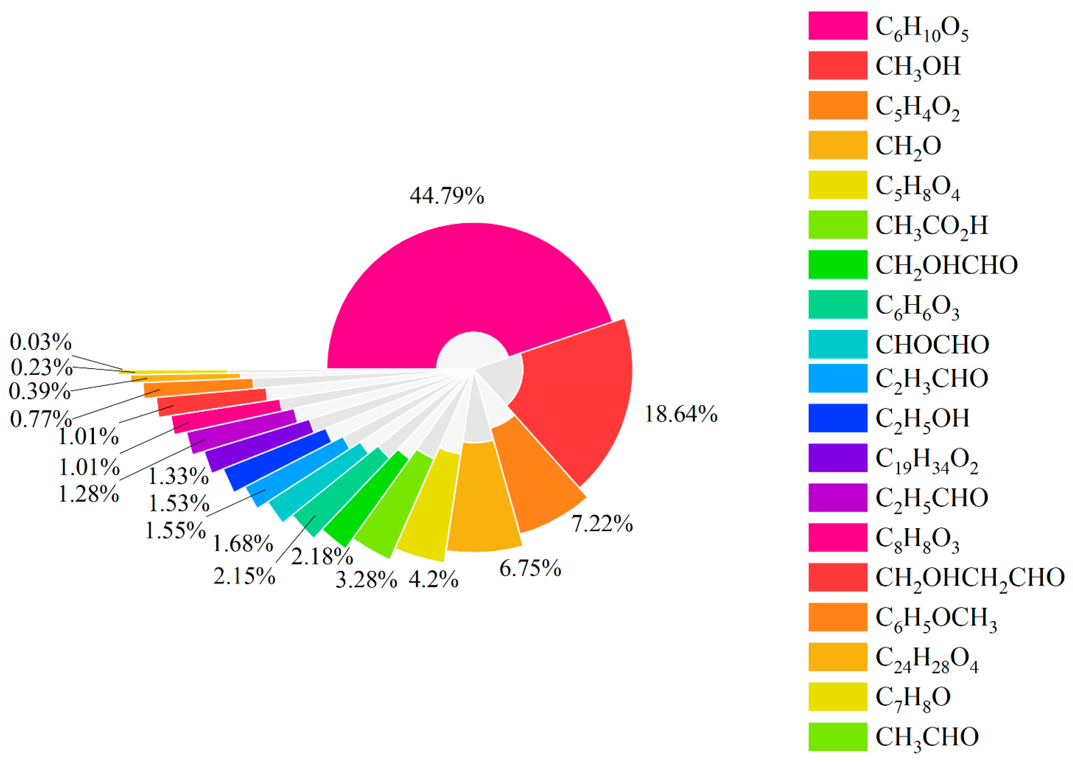
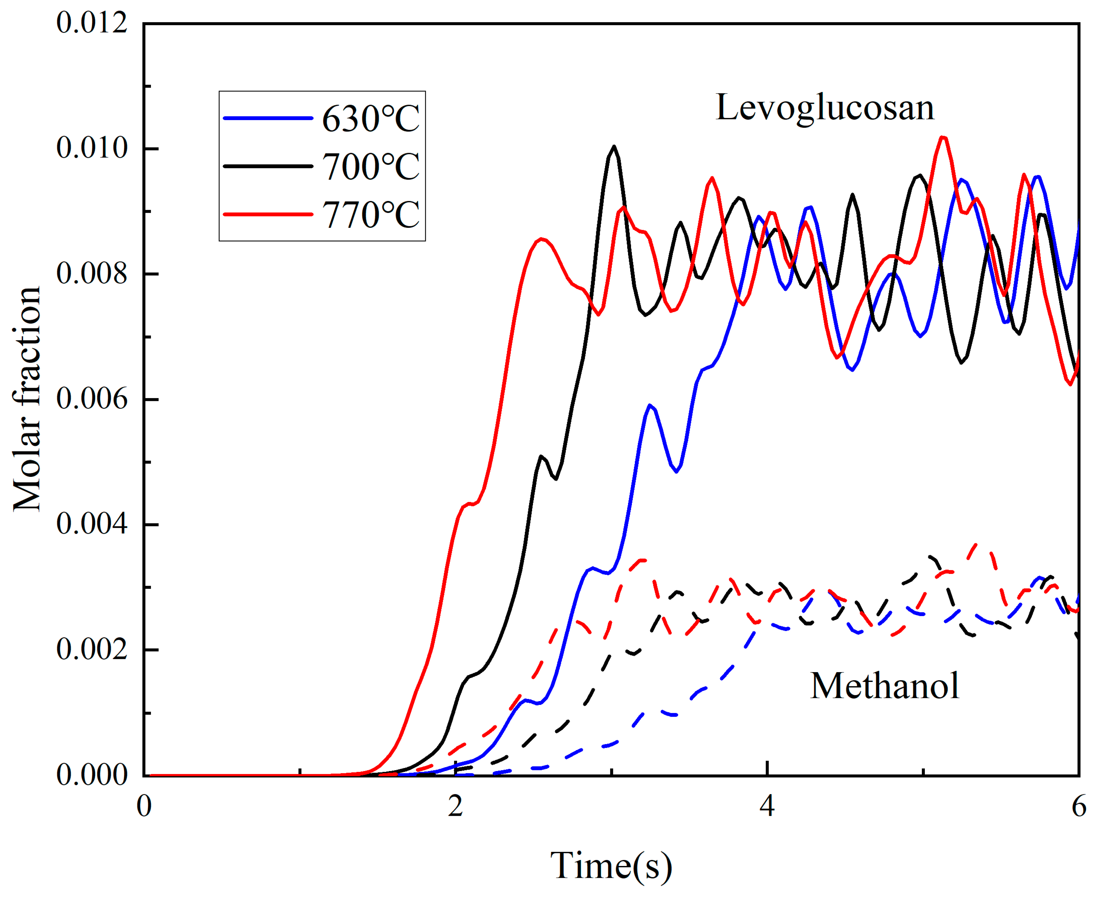
3.2. Tar Component Formation

Tar is mainly generated at medium temperatures and cracked at high temperatures. The chemical model used in this article can analyze the formation of tar components, excluding the stage of tar cracking, which will result in a higher tar content than the actual situation. At the three reaction temperatures considered, the average content of tar changes very little. This indicates that in the preliminary pyrolysis process of biomass, the generated tar components have fully reacted within the simulated temperature range. Figure 5 delineates the tar speciation profile, revealing levoglucosan (C₆H₁₀O₅, 44.79%) as the predominant species, followed by methanol (CH₃OH, 18.64%). These two collectively account for 63.43% of all tar components, highlighting their priority for coking prevention strategies. In addition, furfural (C₅H₄O₂), methanal (CH₂O), and glutaric acid (C₅H₈O₄) account for over 80% of all tar components. This shows the capability of the approximate alternative model to simplify the calculation.

Figure 6 presents the molar fraction curves of the tar components with the two highest contents over time. Within a few seconds, their formation reaches a relatively stable value. Although temperature has little effect on the molar fraction, it influences the formation rate. It can be seen that higher reaction temperatures correspond to steeper slopes and shorter times to peak, indicating that higher temperatures accelerate the reaction kinetics.

3.3. Reaction Rate Analysis

Through simulation, the intensity field of each chemical reaction can be observed at any moment. For example, Figure 7 illustrates the rate of reverse methanation reaction (No. 2 in Table 1), whose products are CO and H₂, during the time period of 8.0–8.5 s. From the comparison between Figure 4 and Figure 7, it can be seen that there is a positive correlation between the concentration of hydrogen and the intensity of R2. They both have an uneven distribution, with a higher concentration on the opposite side of the biomass inlet. Therefore, the distribution of the chemical reaction intensity observed through simulation is also a reference for optimizing.

Next, the effect of temperature on the rate of various chemical reactions in the system was further analyzed using the reaction rate at 700 °C as the benchmark value of 100%, as shown in

Table 4. Effects of temperature on reaction rates (700 °C = 100%).

Reaction Number	630 °C	770 °C
1	86.38%	107.30%
2	38.63%	277.62%
3	106.88%	127.02%
4	53.33%	207.19%
5	114.91%	64.58%
6	125.50%	57.15%
7	113.75%	65.10%
8	144.22%	48.77%
9	24.45%	346.34%
10	175.27%	37.34%
11	25.65%	346.11%
12	165.72%	43.09%
13	30.61%	242.04%
14	128.09%	64.51%
15	142.18%	48.33%
16	141.55%	54.21%
17	185.43%	56.76%
18	145.25%	130.47%
19	124.37%	65.22%
20	143.41%	53.49%
21	148.36%	51.09%
22	122.88%	66.25%
23	11.19%	307.30%
24	66.64%	265.41%
25	30.41%	342.13%
26	124.64%	69.76%
27	112.98%	118.91%
28	44.11%	200.22%
29	116.17%	84.81%
30	151.86%	77.21%
31	8.43%	280.57%
32	8.02%	275.41%
33	7.62%	270.17%
34	196.07%	53.30%
35	4.04%	148.89%
36	146.09%	58.86%

. In gasification reactions, the reactions between CH₄ and water (R2) and char and water (R4) are greatly affected by temperature. The products of both reactions are CO and H₂, which is a major contributor to the increase in the content of CO and H₂ after the reaction temperature rises. In the pyrolysis reaction, the primary decomposition of hemicellulose (R9, R11) and the secondary decomposition of some intermediate products, including intermediate products of hemicellulose (R13), tannins (R24), triglyceride (R23), and its intermediate products (R25), are accelerated significantly. Other significantly accelerated processes are the release of gases adsorbed on solids, such as R28, R31, R32, and R33.

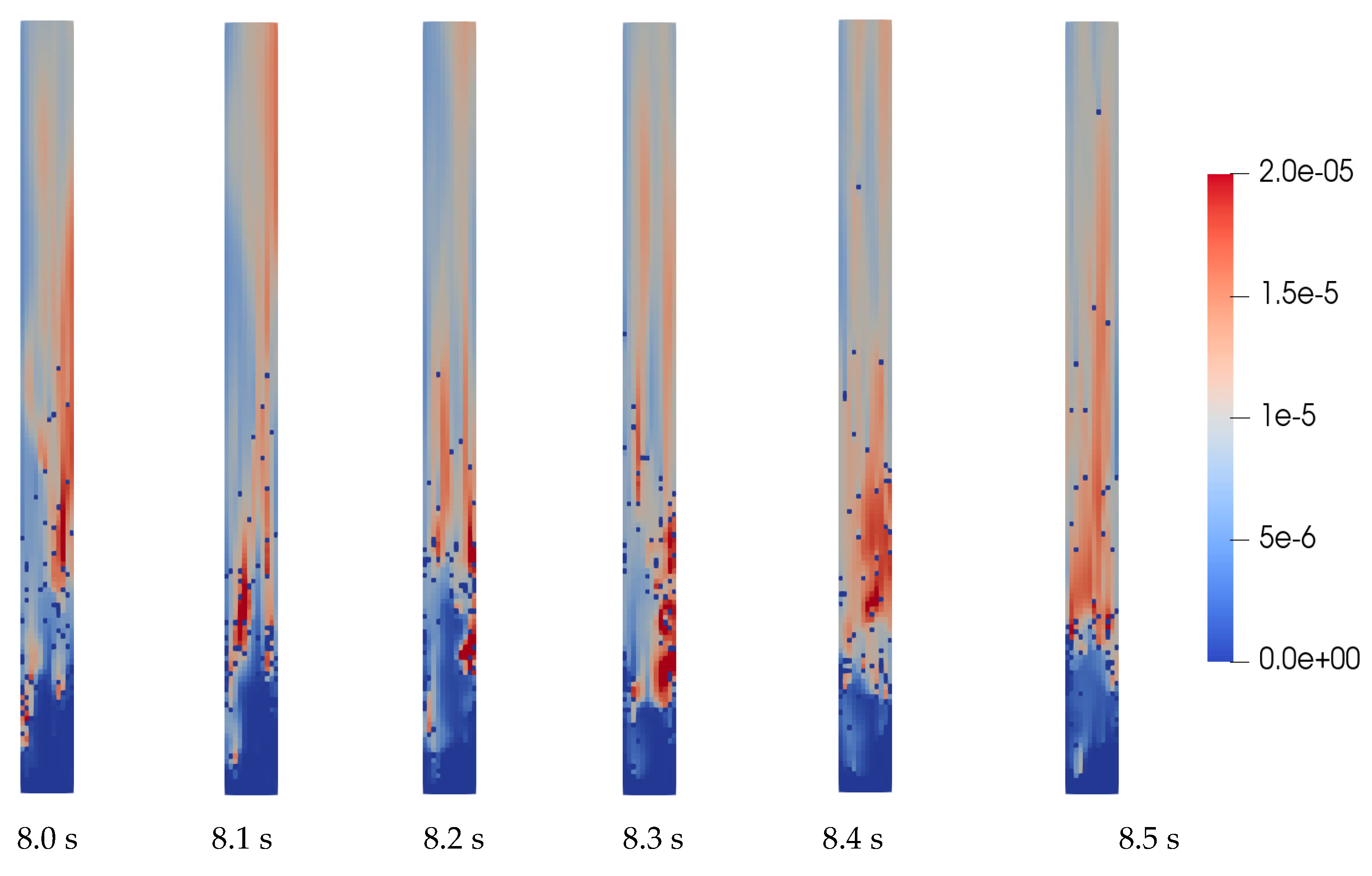
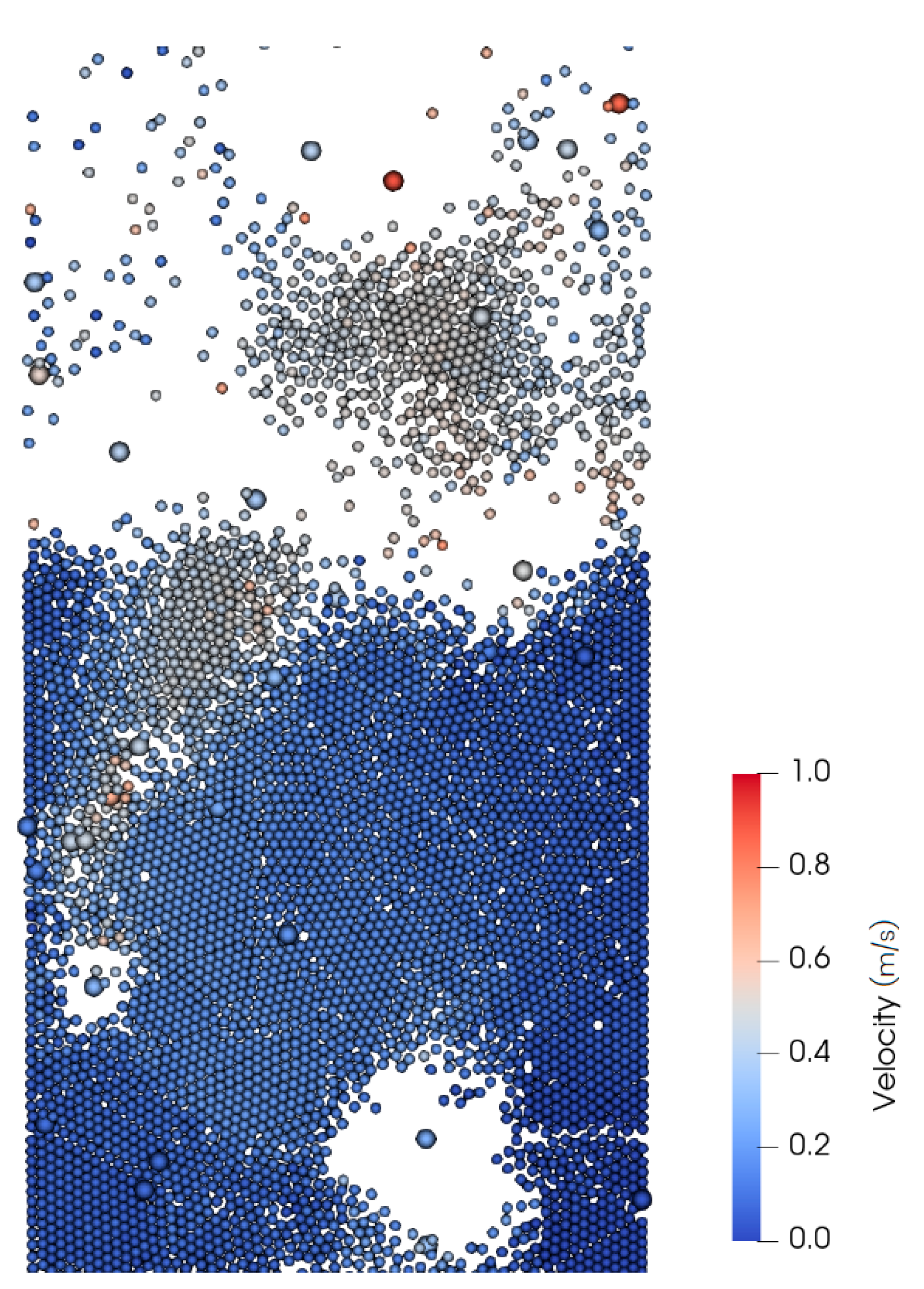
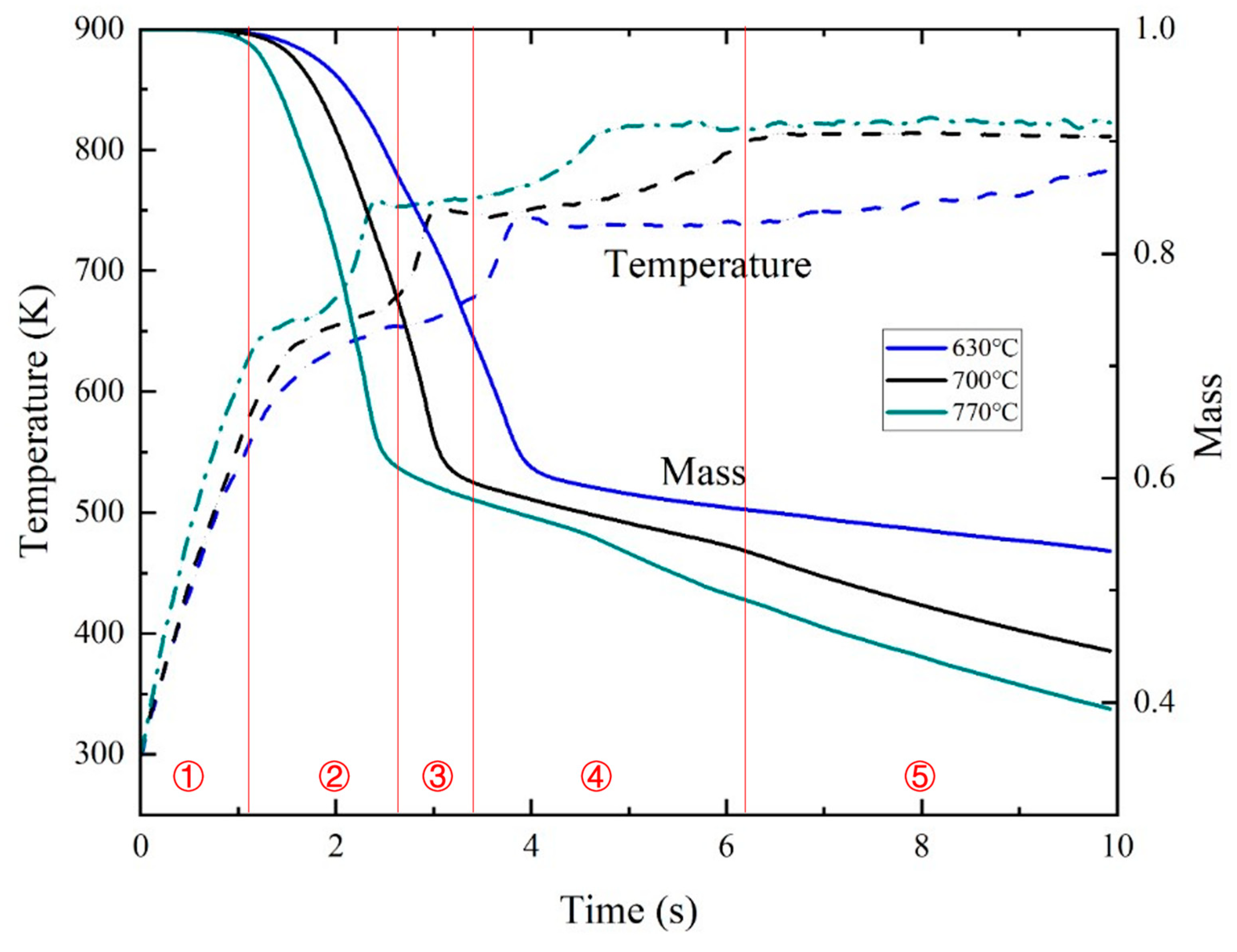
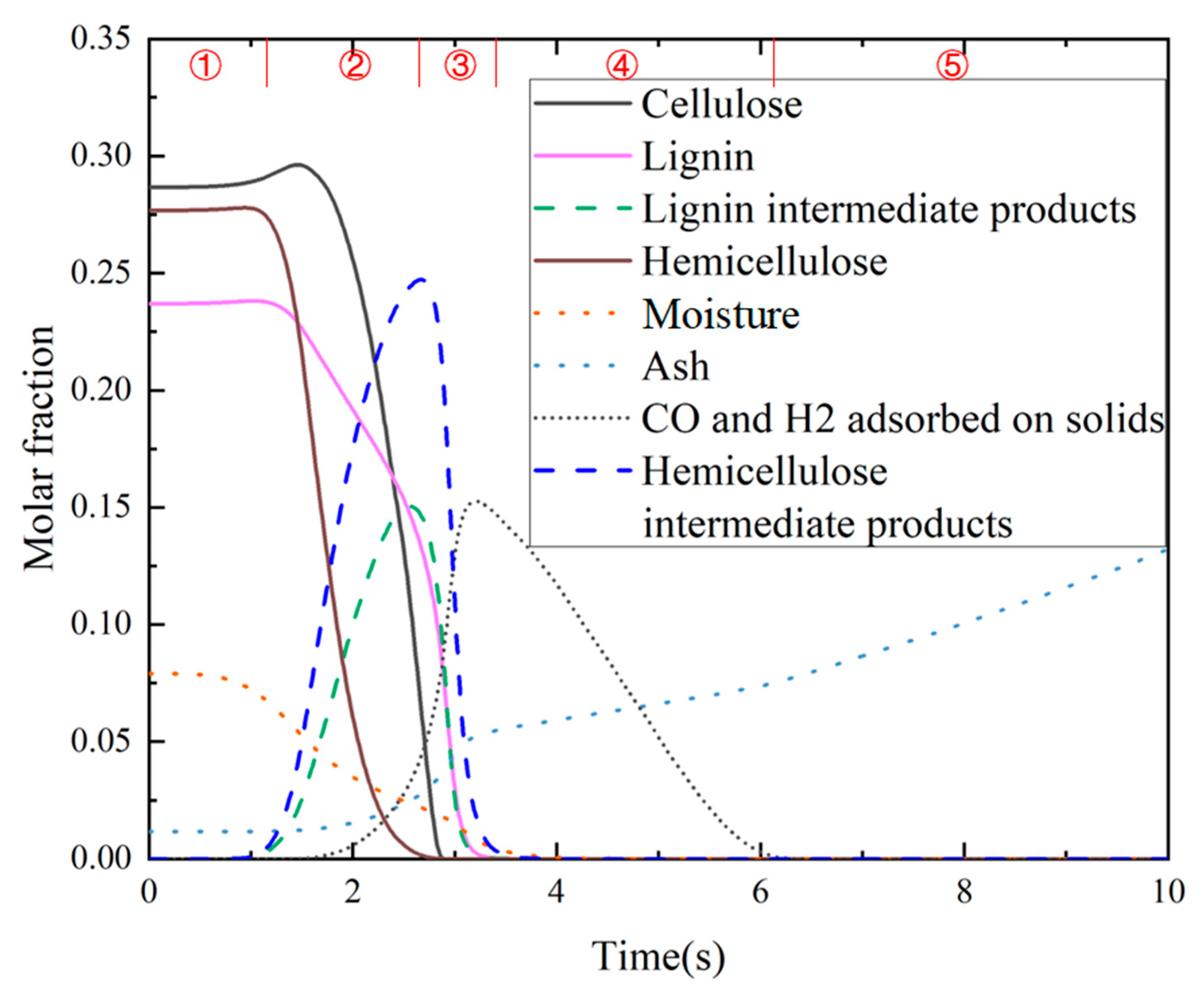
3.4. Particle-Scale Analysis

The DEM method is good at calculating each particle, rather than using cluster approximations; it resolves individual particle trajectories and mesoscale structures (e.g., bubbles) in the fluidized bed (Figure 8). In the figure, larger particles represent biomass, while smaller particles represent sand, and the color represents the particle speed. It can be seen that through the simulation, one can clearly see the particles’ motion and mesoscale structures, such as bubbles in the bubbling fluidized bed, which can reflect the fluid dynamics characteristics of the reactor.

The particle heating and mass loss profiles (Figure 9) demonstrate temperature-dependent pyrolysis kinetics. Obviously, due to the influence of environmental temperature, the heating rate of particles is faster, and the achievable temperature maximum is higher in a hotter reaction environment. Correspondingly, the weight loss rate of particles is also faster at higher temperatures, indicating that the pyrolysis process of biomass particles proceeds more rapidly. Each component can be analyzed, including the generation and disappearance of intermediate products. From Figure 9 and Figure 10, it can be deduced that there is a corresponding relationship between the temperature, mass, and component content changes of the particles. The reaction process is divided into five stages, and the case of 700 °C is taken as an example to provide the content changes of several typical solid components in a particle, as shown in Figure 10.

Phase 1: Moisture evaporation. The temperature of particles gradually increases and the process of moisture drying begins, with the loss of some particle quality.

Phase 2: Primary decomposition. The first stage of pyrolysis reaction occurs, where cellulose, hemicellulose, and lignin begin to decompose and produce intermediate products. The structure of lignin is relatively stable, and its decomposition rate at low temperatures is significantly lower than that of cellulose and hemicellulose, only accelerating at high temperatures. Due to the endothermic nature of the first stage pyrolysis reaction, the rate of temperature rise of the particles is significantly slowed down.

Phase 3: Secondary cracking. This mainly involves secondary reactions, where intermediate products further decompose and release heat, resulting in an accelerated rate of increase in particle temperature.

Phase 4: Adsorbed gas release. This study uniquely resolves gas release dynamics from adsorbed phases on solid surfaces, an often-overlooked process in conventional models. Phase 4 explicitly captures the desorption of gas molecules from char and ash surfaces, a phenomenon rarely quantified in prior studies. This capability stems from the integration of particle-resolved hydrodynamics with semi-detailed surface reaction kinetics, enabling the temporal tracking of adsorbed species (reactions 26–35 in Table 1).

Phase 5: Gasification and ash accumulation. The main reaction that occurs is the gasification reaction. In addition, it can be seen from the gradual increase in ash content that the total weight of particles is still decreasing because ash does not participate in any reaction.

4. Conclusions

This study presents a novel integration of the Discrete Element Method (DEM) with a semi-detailed chemical kinetic mechanism to achieve the particle-resolved modeling of biomass pyrolysis. By coupling CFD-DEM with a 36-step reaction network, the multiscale interactions between particle-scale hydrodynamics and 19 tar components’ formation kinetics under varying temperatures (630–770 °C) are unraveled.

Levoglucosan (44.79%) and methanol (18.64%) are identified as primary tar components, with their formation kinetics governed by temperature. In addition, these, furfural (C₅H₄O₂, 7.22%), methanal (CH₂O, 6.75%), and glutaric acid (C₅H₈O₄, 4.20%) account for over 80% of all tar components.

The proposed model overcomes the limitations of conventional single-step models; successfully captures secondary decomposition pathways at different temperatures; and quantifies the reaction rate changes, such as those seen in triglycerides (R23: 307.30% rate increase at 770 °C) and tannins (R24: 265.41% acceleration).

This work bridges the gap between particle-scale analysis and system-level performance and establishes a paradigm for resolving mesoscale phenomena in thermochemical conversion systems, offering a validated tool for scaling production technologies.

References

1. Ding, S.; Yang, X.; Gan, C.; Qiu, T. Discussion on the New Path of Carbon-Negative Aviation Fuel. Aerosp. Power 2022, 6, 16–19. [Google Scholar]
2. Gan, C.; Ma, Q.; Bao, S.; Wang, X.; Qiu, T.; Ding, S. Discussion of the Standards System for Sustainable Aviation Fuels: An Aero-Engine Safety Perspective. Sustainability 2023, 15, 16905. [Google Scholar] [CrossRef]
3. Nunes, S.M.; Paterson, N.; Herod, A.A.; Dugwell, D.R.; Kandiyoti, R. Tar Formation and Destruction in a Fixed Bed Reactor Simulating Downdraft Gasification: Optimization of Conditions. Energy Fuels 2008, 22, 1955–1964. [Google Scholar] [CrossRef]
4. Sharma, A.; Pareek, V.; Zhang, D. Biomass pyrolysis—A review of modelling, process parameters and catalytic studies. Renew. Sustain. Energy Rev. 2015, 50, 1081–1096. [Google Scholar] [CrossRef]
5. Dilks, R.T.; Monette, F.; Glaus, M. The major parameters on biomass pyrolysis for hyperaccumulative plants—A review. Chemosphere 2016, 146, 385–395. [Google Scholar] [CrossRef]
6. Zhan, X.; Wu, W.; Cui, G. Formation and homogeneous conversion mechanism of biomass pyrolysis tar. Energy Res. Inf. 2019, 35, 125–133. [Google Scholar]
7. Cundall, P.A.; Strack, O.D.L. A discrete numerical model for granular assemblies. Géotechnique 1980, 30, 331–336. [Google Scholar] [CrossRef]
8. Li, C.; Eri, Q. Comparison between two Eulerian-Lagrangian methods: CFD-DEM and MPPIC on the biomass gasification in a fluidized bed. Biomass Convers. Biorefinery 2021, 13, 3819–3836. [Google Scholar] [CrossRef]
9. Oevermann, M.; Gerber, S.; Behrendt, F. Euler–Lagrange/DEM simulation of wood gasification in a bubbling fluidized bed reactor. Particuology 2009, 7, 307–316. [Google Scholar] [CrossRef]
10. Ku, X.; Li, T.; Løvås, T. CFD–DEM simulation of biomass gasification with steam in a fluidized bed reactor. Chem. Eng. Sci. 2015, 122, 270–283. [Google Scholar] [CrossRef]
11. Song, T.; Wu, J.; Shen, L.; Xiao, J. Experimental investigation on hydrogen production from biomass gasification in interconnected fluidized beds. Biomass Bioenergy 2012, 36, 258–267. [Google Scholar] [CrossRef]
12. Ku, X.; Jin, H.; Lin, J. Comparison of gasification performances between raw and torrefied biomasses in an air-blown fluidized-bed gasifier. Chem. Eng. Sci. 2017, 288, 235–249. [Google Scholar] [CrossRef]
13. Ku, X.; Shen, F.; Jin, H.; Lin, J.; Li, H. Simulation of biomass pyrolysis in a fluidized bed reactor using thermally thick treatment. Ind. Eng. Chem. Res. 2019, 58, 1720–1731. [Google Scholar] [CrossRef]
14. Mettler, M.S.; Vlachos, D.G.; Dauenhauer, P.J. Top ten fundamental challenges of biomass pyrolysis for biofuels. Energy Environ. Sci. 2012, 5, 7797–7809. [Google Scholar] [CrossRef]
15. Shafizadeh, F.; Fu, Y.L. Pyrolysis of cellulose. Carbohydr. Res. 1973, 29, 113–122. [Google Scholar] [CrossRef]
16. Bradbury, A.; Sakai, Y.; Shafizadeh, F. A kinetic model for pyrolysis of cellulose. J. Appl. Polym. Sci. 1979, 23, 3271–3280. [Google Scholar] [CrossRef]
17. Ranzi, E.; Cuoci, A.; Faravelli, T.; Frassoldati, A.; Migliavacca, G.; Pierucci, S.; Sommariva, S. Chemical Kinetics of Biomass Pyrolysis. Energy Fuels 2008, 22, 4292–4300. [Google Scholar] [CrossRef]
18. Faravelli, T.; Frassoldati, A.; Migliavacca, G.; Ranzi, E. Detailed kinetic modeling of the thermal degradation of lignins. Biomass Bioenergy 2010, 34, 290–301. [Google Scholar] [CrossRef]
19. Faravelli, T.; Frassoldati, A.; Barker Hemings, E.; Ranzi, E. Multistep Kinetic Model of Biomass Pyrolysis; Springer: London, UK, 2013. [Google Scholar]
20. Ranzi, A.F.; Debiagi, P.E.A.; Frassoldati, A. Mathematical Modeling of Fast Biomass Pyrolysis and Bio-Oil Formation. Note I: Kinetic Mechanism of Biomass Pyrolysis. Acs Sustain. Chem. Eng. 2017, 5, 2867–2881. [Google Scholar] [CrossRef]
21. Ranzi, A.F.; Debiagi, P.E.A.; Frassoldati, A. Mathematical Modeling of Fast Biomass Pyrolysis and Bio-Oil Formation. Note II: Secondary Gas-Phase Reactions and Bio-Oil Formation. Acs Sustain. Chem. Eng. 2017, 5, 2882–2896. [Google Scholar] [CrossRef]
22. Debiagi, P.; Gentile, G.; Cuoci, A.; Frassoldati, A.; Ranzi, E.; Faravelli, T. A predictive model of biochar formation and characterization. J. Anal. Appl. Pyrolysis 2018, 134, 326–335. [Google Scholar] [CrossRef]
23. Lu, L.; Gao, X.; Gel, A.; Wiggins, G.M.; Crowley, M.; Pecha, B.; Shahnam, M.; Rogers, W.A.; Parks, J.; Ciesielski, P.N. Investigating biomass composition and size effects on fast pyrolysis using global sensitivity analysis and CFD simulations. Chem. Eng. J. 2021, 421, 127789. [Google Scholar] [CrossRef]
24. Rapagnà, S.; Jand, N.; Kiennemann, A.; Foscolo, P.U. Steam-gasification of biomass in a fluidised-bed of olivine particles. Biomass Bioenergy 2000, 19, 187–197. [Google Scholar] [CrossRef]
Figure 1. Computational mesh schematic.
Aerospace 12 00477 g001
Figure 2. Experimental setup: (1) gasifier; (2) cyclone; (3) filter; (4) biomass feeder; (5) condenser; (6) blower; (7) gas-meter [24].
Aerospace 12 00477 g002
Figure 3. Temperature-dependent molar fractions of gaseous products.
Aerospace 12 00477 g003
Figure 4. H2 molar fraction profiles at 35 s (630 °C, 700 °C, 770 °C).
Aerospace 12 00477 g004
Figure 5. Proportion of components in tar formation.
Aerospace 12 00477 g005
Figure 6. Molar fraction curves of levoglucosan and methanol at different temperatures.
Aerospace 12 00477 g006
Figure 7. Reverse methanation reaction rates (8.0–8.5 s).
Aerospace 12 00477 g007
Figure 8. An enlarged view of a part in the reactor at 22.5 s.
Aerospace 12 00477 g008
Figure 9. Changes in temperature and normalized mass of a biomass particle at different temperatures.
Aerospace 12 00477 g009
Figure 10. Changes of typical solid components in a biomass particle.
Aerospace 12 00477 g010