Article

A Parameter Self-Tuning Rule Based on Spatial–Temporal Scale for Active Disturbance Rejection Control and Its Application in Flight Test Chamber Systems

1
College of Computer and Data Science, Fuzhou University, Fuzhou 350108, China
2
School of New Engineering Industry, Putian University, Putian 351100, China
3
Huida Technology Development Co., Ltd., Fuzhou 350108, China
4
School of Automation, China University of Geosciences (Wuhan), Wuhan 430074, China
5
Science and Technology on Altitude Simulation Laboratory, AECC Sichuan Gas Turbine Establishment, Mianyang 621703, China
6
School of Mechanical Engineering and Automation, Fuzhou University, Fuzhou 350108, China
*
Author to whom correspondence should be addressed.
Aerospace 2025, 12(6), 465; https://doi.org/10.3390/aerospace12060465
Submission received: 15 March 2025 / Revised: 6 May 2025 / Accepted: 19 May 2025 / Published: 23 May 2025
(This article belongs to the Section Aeronautics)

Abstract

:
Active disturbance rejection control (ADRC) emerges as a promising control approach due to its partial model-based characteristics and strong disturbance rejection capabilities. Nevertheless, it is a difficult problem to tune various parameters of ADRC in practical applications. To address the challenge of parameter tuning, this work develops a parameter self-tuning rule based on spatial–temporal scale transformations to simplify the tuning process and enhance its control performance. In particular, based on the transformations of spatial–temporal scale, the parameter tuning relationships for ADRC’s components, including tracking differentiator (TD), extended state observer (ESO) and feedback controller, are provided for a second-order nonlinear system. Numerical simulations show that the proposed method can conveniently and effectively provide a set of well-tuned parameters for ADRC to boost the efficiency of control. Finally, the proposed parameter tuning rule is applied to the intake pressure control of the flight test chamber system, further validating its effectiveness. The results demonstrate that the ADRC with the proposed parameter self-tuning method significantly improves the precision of the intake pressure under different operating conditions, thereby ensuring the reliability of aeroengine flight tests.

1. Introduction

Due to its simple structure and model-free characteristic, proportional–integral–derivative (PID) or PI has been widely used in different control scenarios [1,2]. However, the performance of control systems can be seriously affected by the unknown external disturbances and system uncertainties. To improve the control performance, the recent decade witnessed a booming development of numerous anti-disturbance control approaches in various industrial systems [3,4,5].
Active disturbance rejection control (ADRC), as a promising anti-disturbance approach, provides high-precision control in the presence of unknown disturbances or uncertainties [6,7,8]. By utilizing an extended state observer (ESO) to dynamically estimate and compensate for total disturbances, ADRC enables effective control without relying on accurate system models [9,10]. Especially with its simple structure and strong anti-disturbance capabilities, linear ADRC has been applied broadly in various industrial systems, such as power systems [11,12], motion control systems [13,14], and aerospace control systems [15,16,17,18]. Similar to other observer-based control methods, the performance of ADRC strongly depends on the selection of the observer gain and feedback controller parameters [19,20]. In complex dynamic environments, the selection of these parameters directly influences system response, disturbance rejection, and robustness [21,22]. A reasonable parameter tuning rule can significantly improve response speed, reduce overshoot and enhance system stability. Traditionally, parameter tuning is made using trial-and-error methods, which requires continuously adjusting the parameters to achieve satisfactory performance [23,24]. Such a tuning approach is time-consuming and cannot guarantee control performance.
To simplify the parameter tuning of ADRC and improve its control performance, numerous parameter tuning methods have been proposed. For instance, Yuan et al. analyzed the frequency band characteristics and noise transmission features of a linear ADRC and presented an engineering configuration method for ADRC [25]. Liang et al. used the least squares method to identify the parameter b 0 (i.e., the estimation value of the closed-loop system control gain b under the ADRC paradigm) in response to the difficulty of tuning the parameter b 0 of the ADRC [26]. Chen et al. developed a data-driven ADRC iterative tuning method using empirical relations and the iterative feedback tuning stochastic approximation algorithm, achieving a suitable balance between performance and robustness [27]. The aforementioned methods have their pros and cons and can optimize the parameter tuning of ADRC in some aspects. To further enhance the the adaptability of parameter tuning, inspired by [28,29,30], the parameter tuning rules based on spatial–temporal scale transformations offer a novel way to adjust parameters. By effectively and meticulously segmenting the system and its signals, such methods enable a more detailed description of the system and signals, leading to more efficient tuning of parameters.
Based on the transformations of spatial–temporal scale, this work proposes an efficient parameter tuning rule for ADRC to simplify the tuning process and enhance its control performance. First, the structure of ADRC and the definition of a system temporal scale are presented. For a second-order nonlinear system, a parameter tuning rule for ADRC based on spatial–temporal scale transformations is derived. Simulation results preliminarily validate the effectiveness of this parameter tuning rule in each component of ADRC and its overall parameter tuning process. Finally, the proposed tuning rule is successfully applied to the intake pressure control of the flight test chamber system under two different test conditions. Test results demonstrate that the ADRC based on the proposed method can significantly improve the intake pressure control performance. More importantly, for multi-condition aeroengine flight tests, as long as the ADRC parameters are tuned for one condition, preliminary ADRC parameters for other conditions can be directly obtained by the proposed method, which significantly simplifies the tuning process.
The remainder of this work is organized as follows. The preliminaries are presented in Section 2. The main results are presented in Section 3, where a parameter tuning rule based on spatial–temporal scale is discussed for the TD, ESO and overall ADRC. Numerical simulations are presented in Section 4, which demonstrate the effectiveness of the proposed parameter tuning rule. In Section 5, the test results are given. Finally, the work is summarized in Section 6.

2. Preliminaries

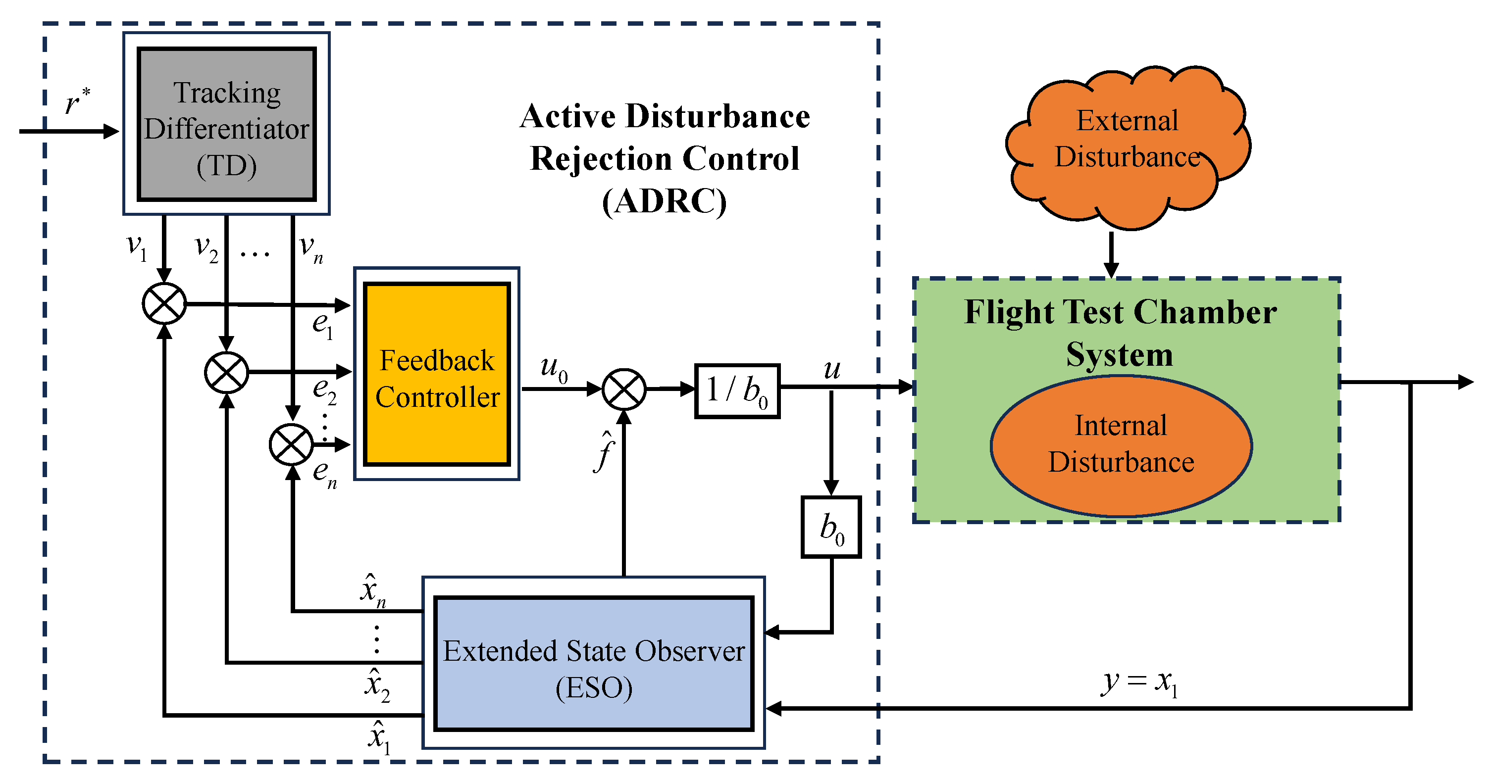
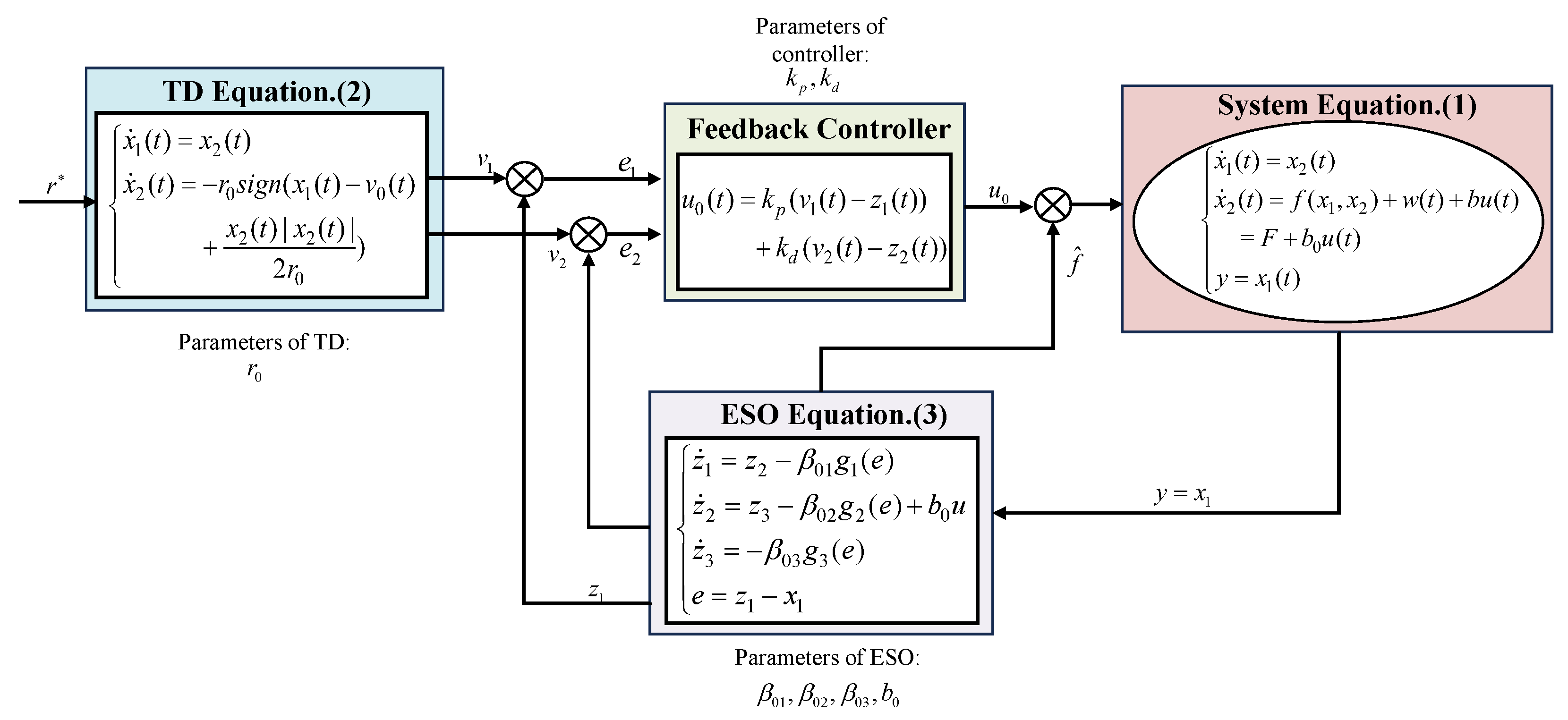
2.1. Brief Introduction of ADRC

As shown in Figure 1, the basic structure of an ADRC based on the intake pressure control for the flight test chamber system includes a tracking differentiator (TD), an ESO and a feedback controller [6].
Consider a second-order nonlinear system:
x ˙ 1 ( t ) = x 2 ( t ) x ˙ 2 ( t ) = f ( x 1 , x 2 , t ) + w ( t ) + b u ( t ) = F + b 0 u ( t ) y = x 1 ( t )
where x 1 and x 2 are the system states, w is the unknown external disturbance, b is the control gain, u is the system input, and y = x 1 is the system output. The total disturbance F = f ( x 1 , x 2 , t ) + w ( t ) + ( b b 0 ) u ( t ) can be extended as a new system state, defined as x 3 . The symbol b 0 is the estimated value of b. For system (1), the time optimal control-based TD (TOC-TD) is established as [29]
v ˙ 1 ( t ) = v 2 ( t ) v ˙ 2 ( t ) = r 0 sgn ( v 1 ( t ) v 0 ( t ) + v 2 ( t ) | v 2 ( t ) | 2 r 0 )
where v 1 and v 2 are the tracking signals of any given signals v 0 and its derivative, respectively. The parameter r 0 is proportional to the tracking speed of the differentiator. The TD is responsible for generating a smooth reference signal from potentially noisy input signals and for providing accurate estimates of the signal and its derivative (velocity). One feasible third-order ESO can be designed as [7]
z ˙ 1 ( t ) = z 2 ( t ) β 01 g 1 ( e ( t ) ) z ˙ 2 ( t ) = z 3 ( t ) β 02 g 2 ( e ( t ) ) + b 0 u ( t ) z ˙ 3 ( t ) = β 03 g 3 ( e ( t ) ) e ( t ) = z 1 ( t ) x 1 ( t )
where z 1 , z 2 and z 3 are observer states estimating system state variables x 1 and x 2 and total disturbances F, respectively. The symbol e is the observer error. The symbol g i ( e ) , i = 1 , 2 , 3 is the feedback function of error. The parameter β 0 i , i = 1 , 2 , 3 is the observer gain. The ESO is a core component that estimates both the system states (such as position, velocity) and total disturbances in real-time. When the obtained estimated value of total disturbances F is utilized for dynamic compensation, the control law can be deduced as
u ( t ) = u 0 ( t ) z 3 ( t ) b 0
where the control component u 0 can be obtained using various mature feedback controllers. For example, in a linear ADRC method, a proportional–derivative (PD) controller is selected as the feedback controller; then, one has u 0 ( t ) = k p ( v 1 ( t ) z 1 ( t ) ) k d z 2 ( t ) . The parameters k p and k d are the gains of proportional and derivative control, respectively.

2.2. System Spatial–Temporal Scale

The temporal scale is the measure of the speed of action or response for different systems. The definition of temporal scale is as follows:
Definition 1
([29,31]). For a general second-order system x ¨ 1 = f ( x 1 , x 2 , t ) , the temporal scale of the system can be defined as
p = 1 M
where the symbol M = max | x | c 1 , | x 2 | c 2 | f ( x 1 , x 2 , t ) | . The constants c 1 , c 2 are the operating range of the system states x 1 , x 2 , respectively. When the input u ( t ) is fixed, the system’s temporal scale will be determined by its system states and the process values of the input. Similarly, for system x 1 ( n ) = f ( x 1 , x 2 , , x n , t ) , the temporal scale can be written as p = 1 / M 1 / n . In addition, for the system output y = A 1 x 1 ( t ) , its spatial scale can be defined as A 1 .
Remark 1. 
The defined system temporal scale is essentially the maximum value of the highest-order derivative within the system operating range, that is, the temporal scale focuses on the rate of change of the system’s highest-order derivative.

3. Main Results: The Proposed ADRC Parameter Tuning Rule

In this section, spatial–temporal scale transformations are applied to the TD, ESO and feedback controller. Further, a novel parameter tuning rule for ADRC is obtained. The control parameters to be adjusted for TD, ESO and feedback controller in the ADRC control of the flight test chamber system are shown in Figure 2.

3.1. Spatial–Temporal Scale Transformations of TD

The given signal v 0 for TD is set as v 0 ( t ) = μ 0 sin ( w 0 t ) . According to the trial-and-error method, a proper value of the parameter r 0 is obtained. When the amplitude μ 0 and frequency w 0 of v 0 are changed, the given signal becomes v n ( t ) = A μ 0 sin ( k w 0 t ) . By applying the spatial–temporal scale transformations to the differentiator, the parameter of v n can be calculated. The transformations are designed as follows:
t = k τ v ^ 1 ( τ ) = A v 1 ( t ) v ^ 2 ( τ ) = A k v 2 ( t )
where k and A are the ratios of the spatial–temporal scale of v 0 and v n , respectively. The symbols v ^ 1 ( τ ) and v ^ 2 ( τ ) are the spatial–temporal scale transformations of v 1 ( t ) and v 2 ( t ) , respectively. By Equations (2) and (6), one has
d v 1 d τ = d v 1 d t d t d τ = k v ˙ 1 d v 2 d τ = d v 2 d t d t d τ = k v ˙ 2
and
d v ^ 1 d τ = A d v 1 d τ = A k v ˙ 1 = A k v 2 d v ^ 2 d τ = A k d v 2 d τ = A k 2 v ˙ 2 = A k 2 r 0 s g n ( v 1 ( t ) v 0 ( t ) + v 2 ( t ) | v 2 ( t ) | 2 r 0 )
Combing Equations (6) and (8), we have
v ^ ˙ 1 ( τ ) = v ^ 2 ( τ ) v ^ ˙ 2 ( τ ) = A k 2 r 0 s i g n ( v ^ 1 ( τ ) v n ( τ ) + v ^ 2 ( τ ) | v ^ 2 ( τ ) | 2 A k 2 r 0 )
where v n ( τ ) = A v 0 ( τ ) = A μ 0 sin ( k w 0 τ ) . According to Equation (9), the new parameter of TD for the actual signal v n is as
r n = A k 2 r 0
where r 0 is the parameter of the actual signal v n . From Equation (10), it evident that the parameter of TD r 0 for the reference signal v 0 is selected; the parameter r n for the actual signal v n can be quickly determined based on the spatial–temporal scale transformation, ensuring reliable signal tracking performance.

3.2. Spatial–Temporal Scale Transformations of ESO and Feedback Controller

By Equation (1), the total disturbances F of the original system is defined as x 3 = F . When its amplitude and frequency change, the total disturbances become x ^ 3 = A F ( k τ ) . To obtain the new parameters of ESO, the spatial–temporal scale transformations of the original system and ESO are as follows:
t = k τ x ^ 1 ( τ ) = A k 2 x 1 ( t ) x ^ 2 ( τ ) = A k x 2 ( t )
t = k τ z ^ 1 ( τ ) = A k 2 z 1 ( t ) z ^ 2 ( τ ) = A k z 2 ( t ) z ^ 3 ( τ ) = A z 3 ( t )
where k and A are the ratios of the spatial–temporal scale of x 3 and x ^ 3 , respectively. According to Equation (11), one has
d x 1 d τ = d x 1 d t d t d τ = k x ˙ 1 d x 2 d τ = d x 2 d t d t d τ = k x ˙ 2
and
d x ^ 1 d τ = A k 2 d x 1 d τ = A k 2 k x ˙ 1 = A k x 2 d x ^ 2 d τ = A k d x 2 d τ = A k k x ˙ 2 = A ( x 3 + b 0 u )
By Equations (13) and (14), the controlled system (1) is transformed into
x ^ ˙ 1 ( τ ) = x ^ 2 ( τ ) x ^ ˙ 2 ( τ ) = A x 3 ( τ ) + A b 0 u ( τ ) y = x ^ 1 ( τ )
Using Equations (3) and (12), we have
d z 1 d τ = d z 1 d t d t d τ = k z ˙ 1 d z 2 d τ = d z 2 d t d t d τ = k z ˙ 2 d z 3 d τ = d z 3 d t d t d τ = k z ˙ 3
and
d z ^ 1 d τ = A k 2 d z 1 d τ = A k z ˙ 1 ( t ) = z ^ 2 ( τ ) β 010 g 1 ( e ( τ ) ) d z ^ 2 d τ = A k d z 2 d τ = A z ˙ 2 ( t ) = z ^ 3 ( τ ) β 020 g 1 ( e ( τ ) ) + b 01 u ( τ ) d z ^ 3 d τ = A d z 3 d τ = A k z ˙ 3 ( t ) = β 030 g 1 ( e ( τ ) )
By Equation (17), for system (15), the ESO (3) is rewritten as
z ^ ˙ 1 ( τ ) = z ^ 2 ( τ ) β 010 g 1 ( e ( τ ) ) z ^ ˙ 2 ( τ ) = z ^ 3 ( τ ) β 020 g 2 ( e ( τ ) ) + b 01 u ( τ ) z ^ ˙ 3 ( τ ) = β 030 g 3 ( e ( τ ) )
where the parameters of ESO are the β 010 = A k β 01 , β 020 = A β 02 , β 030 = A k β 03 and b 01 = A b 0 , respectively. If a set of parameters β 0 i , i = 1 , 2 , 3 enable the ESO (3) to effectively estimate the system (1) states and total disturbances F, the observer (18) with parameters β 0 i 0 , i = 1 , 2 , 3 obtained by the spatial–temporal scale transformation can also guarantee the estimation capability of the new system (15). Similar to TD and ESO, as the characteristic of the controlled system change, the parameters of feedback controller should be adjusted to satisfy system performance. Based on the same principle of spatial–temporal scale transformations, the feedback controller u 0 is further described as
u 0 ( τ ) = k p 0 e 1 ( τ ) k d 0 e 2 ( τ )
where the parameters of feedback controller k p 0 = A k p , k d 0 = ( A / k ) k d .

3.3. ADRC Parameter Tuning Rule

Combing the TD (9), ESO (18) and feedback controller (19), the ADRC controller is as follows:
v ^ ˙ 1 ( τ ) = v ^ 2 ( τ ) v ^ ˙ 2 ( τ ) = r n s i g n ( v ^ 1 ( τ ) v n ( τ ) + v ^ 2 ( τ ) | v ^ 2 ( τ ) | 2 r n ) z ^ ˙ 1 ( τ ) = z ^ 2 ( τ ) β 010 g 1 ( e ( τ ) ) z ^ ˙ 2 ( τ ) = z ^ 3 ( τ ) β 020 g 2 ( e ( τ ) ) + b 01 u ( τ ) z ^ ˙ 3 ( τ ) = β 030 g 3 ( e ( τ ) ) u 0 ( τ ) = k p 0 e 1 ( τ ) k d 0 e 2 ( τ ) e 1 ( τ ) = v ^ 1 ( τ ) z ^ 1 ( τ ) , e 2 ( τ ) = z ^ 2 ( τ ) u ( τ ) = u 0 ( τ ) z ^ 3 b 01
Following the principle of separation design [4], the preceding sections have systematically investigated the TD, ESO and feedback controller based on spatial–temporal scale transformations. Integrating these three components, the parameter tuning rule of ADRC is concluded as
r n = A k 2 r 0 β 010 = A k β 01 , β 020 = A β 02 , β 030 = A k β 03 , b 01 = A b 0 k p 0 = A k p , k d 0 = A k k d
In addition, based on the above analysis, the tuning process of ADRC for the flight test chamber system is illustrated in Figure 3.
Remark 2. 
The difference between TD and ESO is that TD is model-free, while ESO is weakly model-based (e.g., system order). Therefore, when spatial–temporal scale transformations are applied to the ESO module of ADRC, both the original system and ESO must be transformed simultaneously.

4. Simulation Results

The numerical simulations are conducted on the TD, ESO and overall ADRC to validate the effectiveness of the proposed parameter tuning rule.

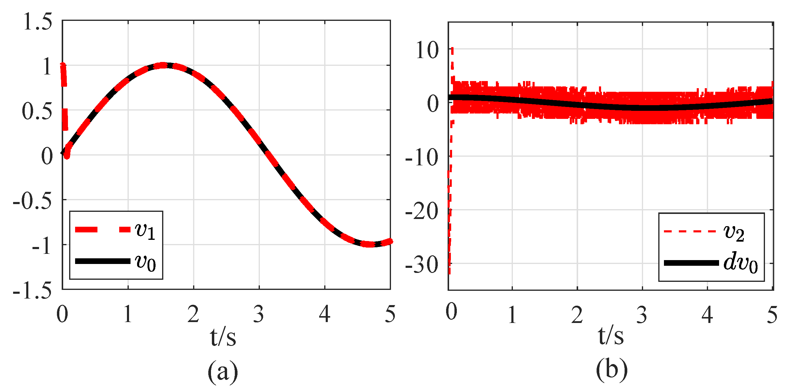
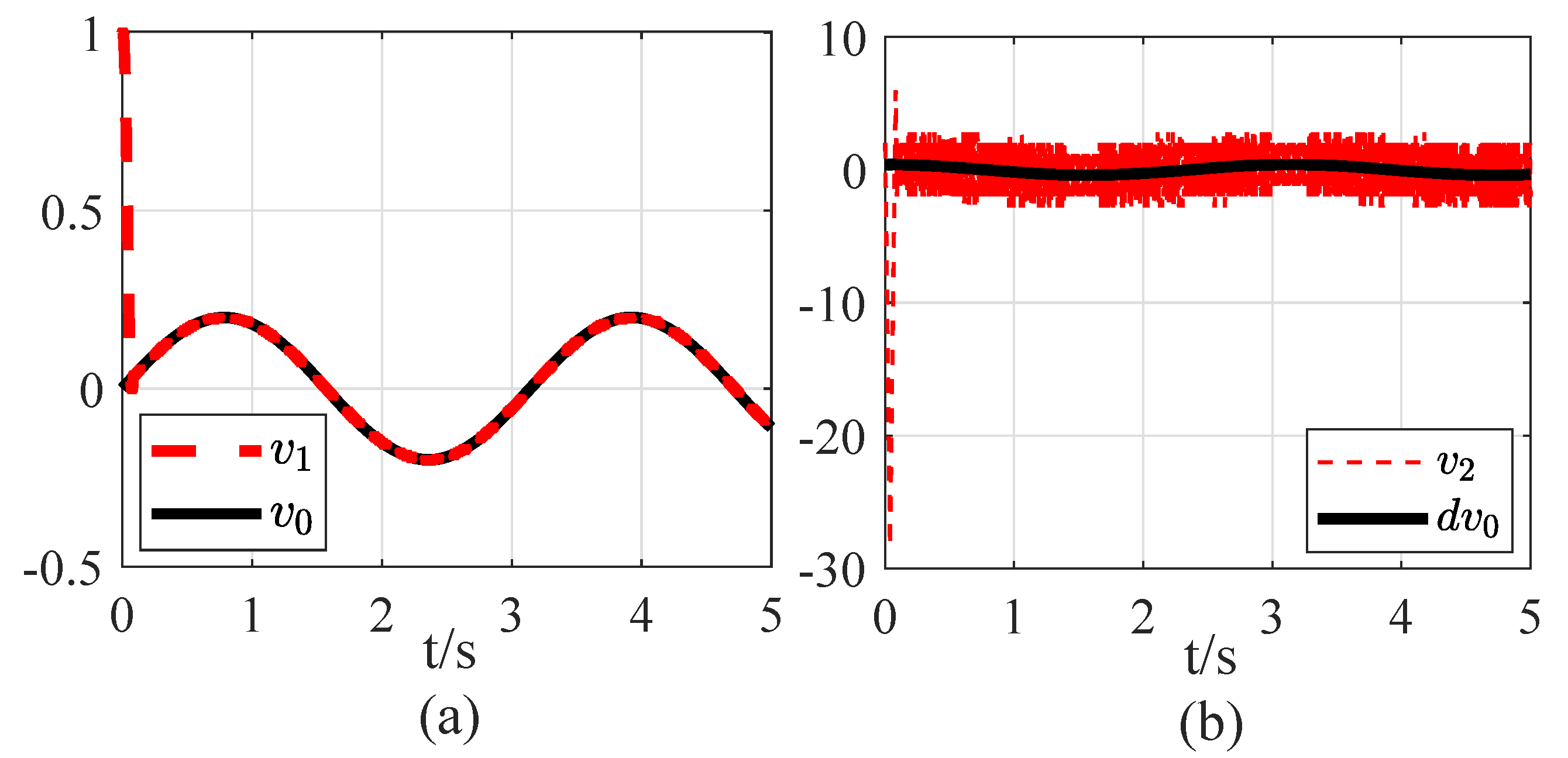
4.1. Signal Tracking and Derivative Acquisition of TD

First, the same simulation environment is adopted in the Matlab program. Specifically, the system sampling period is set as h = 0.02 s and the total simulation time is configured as t = 5 s. The original signal is set as v 0 ( t ) = μ 0 sin ( w 0 t ) , where μ 0 = 1 and w 0 = 1 are the amplitude and frequency of input signal, respectively. The corresponding derivative of v 0 ( t ) is d v 0 ( t ) / d ( t ) = μ 0 w 0 cos ( w 0 t ) . The parameter of TD (2) is selected as r 0 = 1000 by the trial-and-error method to ensure the effective signal tracking and differentiation acquisition. When the amplitude and frequency increment of the original signal v 0 ( t ) change, the new signal is v n ( t ) = A μ 0 sin ( k w 0 t ) , A = 0.2 , k = 2 , μ 0 = 1 , w 0 = 1 . According to the spatial–temporal scale transformation, the parameter of TD (9) can be calculated as r n = 800. The simulation results of signal tracking and differentiation acquisition are shown in Figure 4 and Figure 5.
From Figure 4 and Figure 5, the simulation results demonstrate that when the TD parameter of the original signal v 0 ( t ) is properly selected, the signal tracking and differentiation acquisition capabilities of TD are guaranteed for the new input signal v n ( t ) . Therefore, based on the proposed parameter tuning rule, the obtained new parameter of TD is effective.

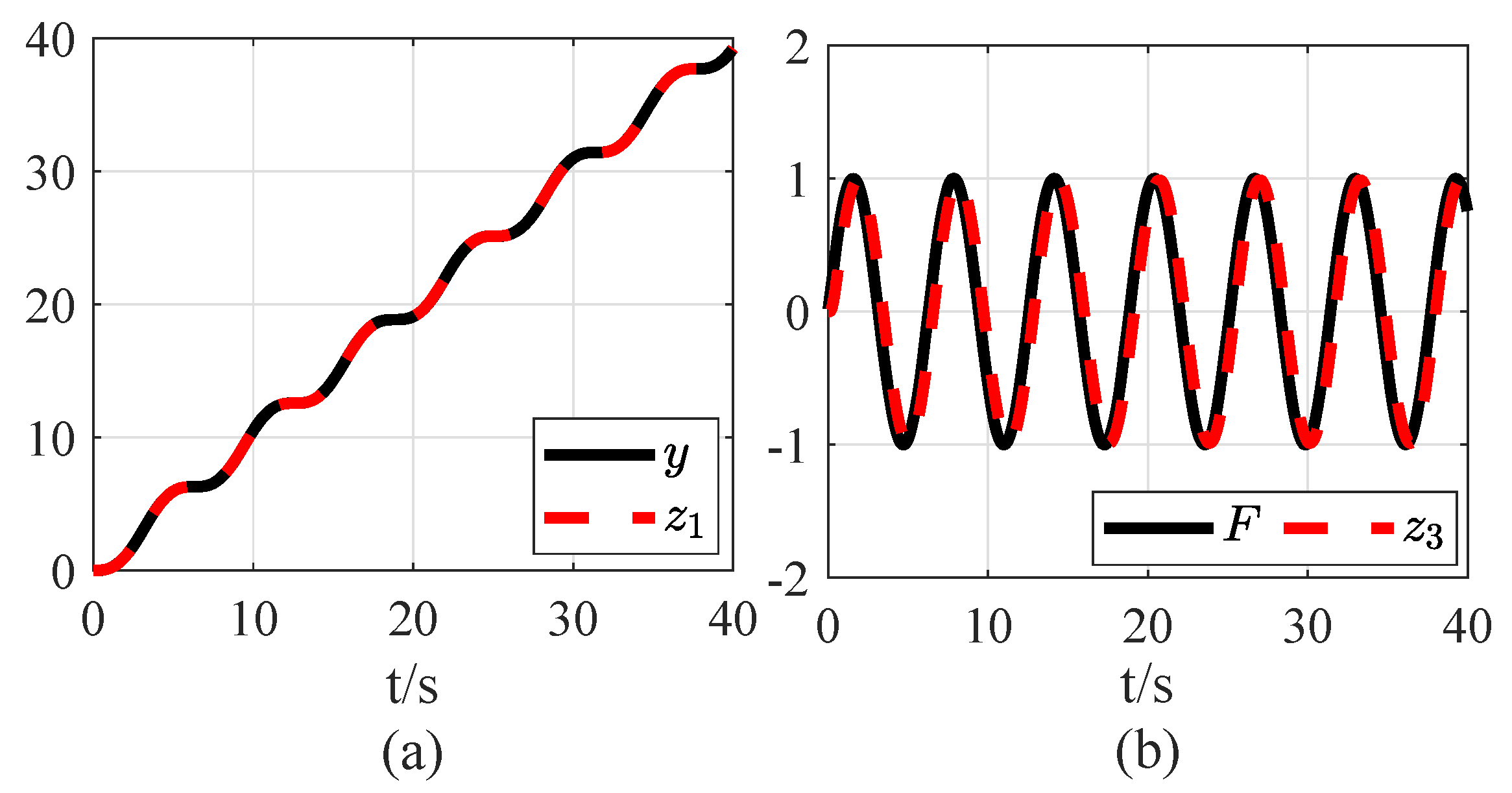
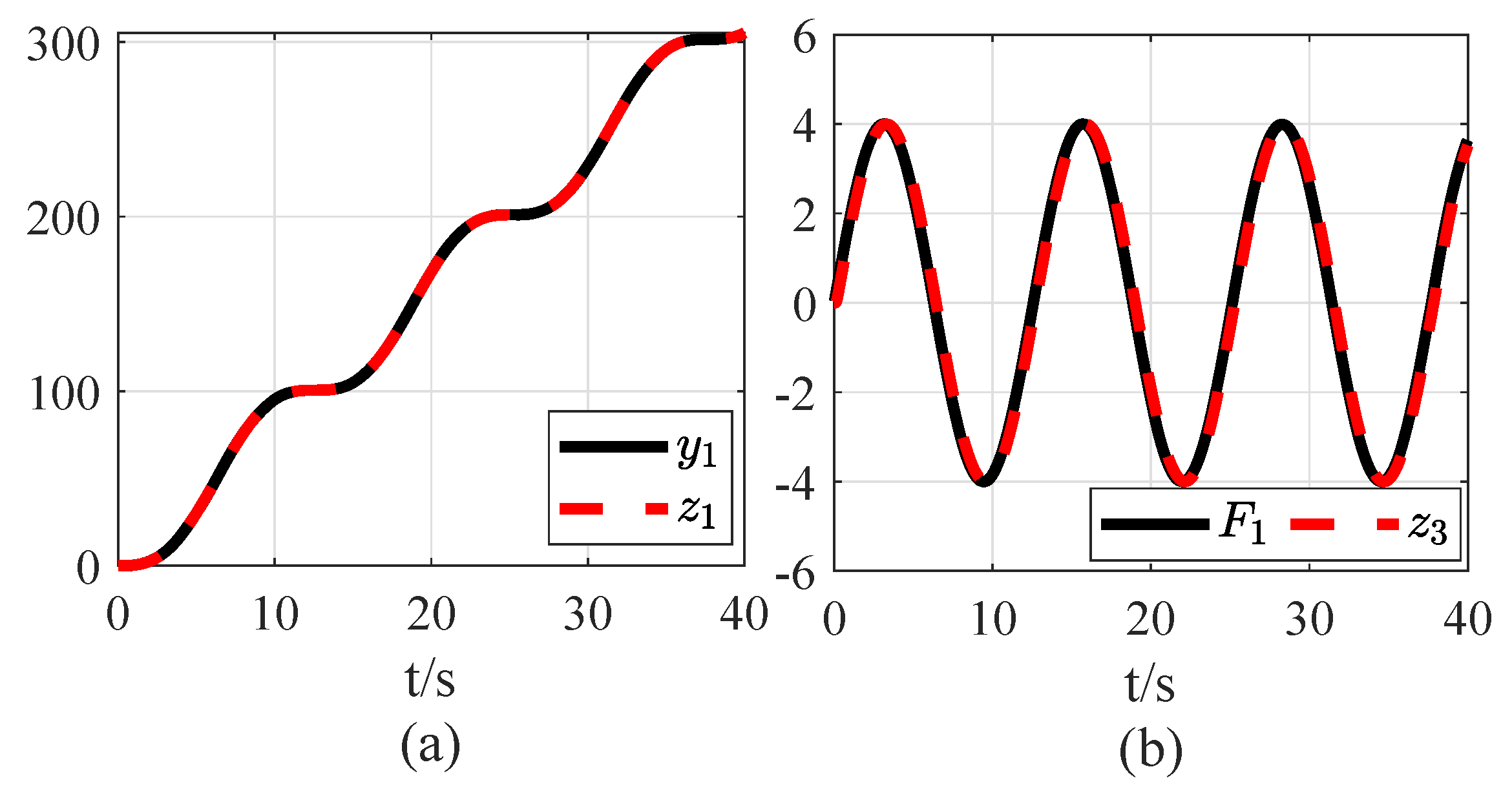
4.2. System States and Disturbance Estimation of ESO

The simulation environment is consistently implemented in Matlab, with the system sampling period h = 0.02 s and the total simulation time t = 40 s. In addition, the total disturbance F of the original system (1) is set as F = μ 0 sin ( w 0 t ) , μ 0 = 1 , w 0 = 1 , and there is no known input. As an example of parameter tuning for the linear ESO, the observation error function is selected as g i ( e ) = e , i = 1 , 2 , 3 . The system states and total disturbance estimation capabilities of ESO are further investigated. By the trial-and-error method, the bandwidth of the observer is given as ω 0 = 10 . Therefore, based on the bandwidth configuration method, the gains of ESO are selected as β 01 = 3 ω 0 = 30 , β 02 = 3 ω 0 2 = 300 , β 03 = 3 ω 0 3 = 3000 . When the total disturbances F change to F 1 = A sin ( k w 0 t ) , A = 4 μ 0 , k = 0.5 , the new parameters of ESO, based on the obtained parameter tuning relationship, are given as β 010 = 240 , β 020 = 1200 , β 030 = 6000 .
As shown in Figure 6 and Figure 7, based on the above two sets of simulation results, the parameters of ESO (3) for the original total disturbances F are determined. Under the same input conditions, for the transformed total disturbances F 1 , the parameters of ESO (18) are obtained to guarantee the disturbance estimation capability.

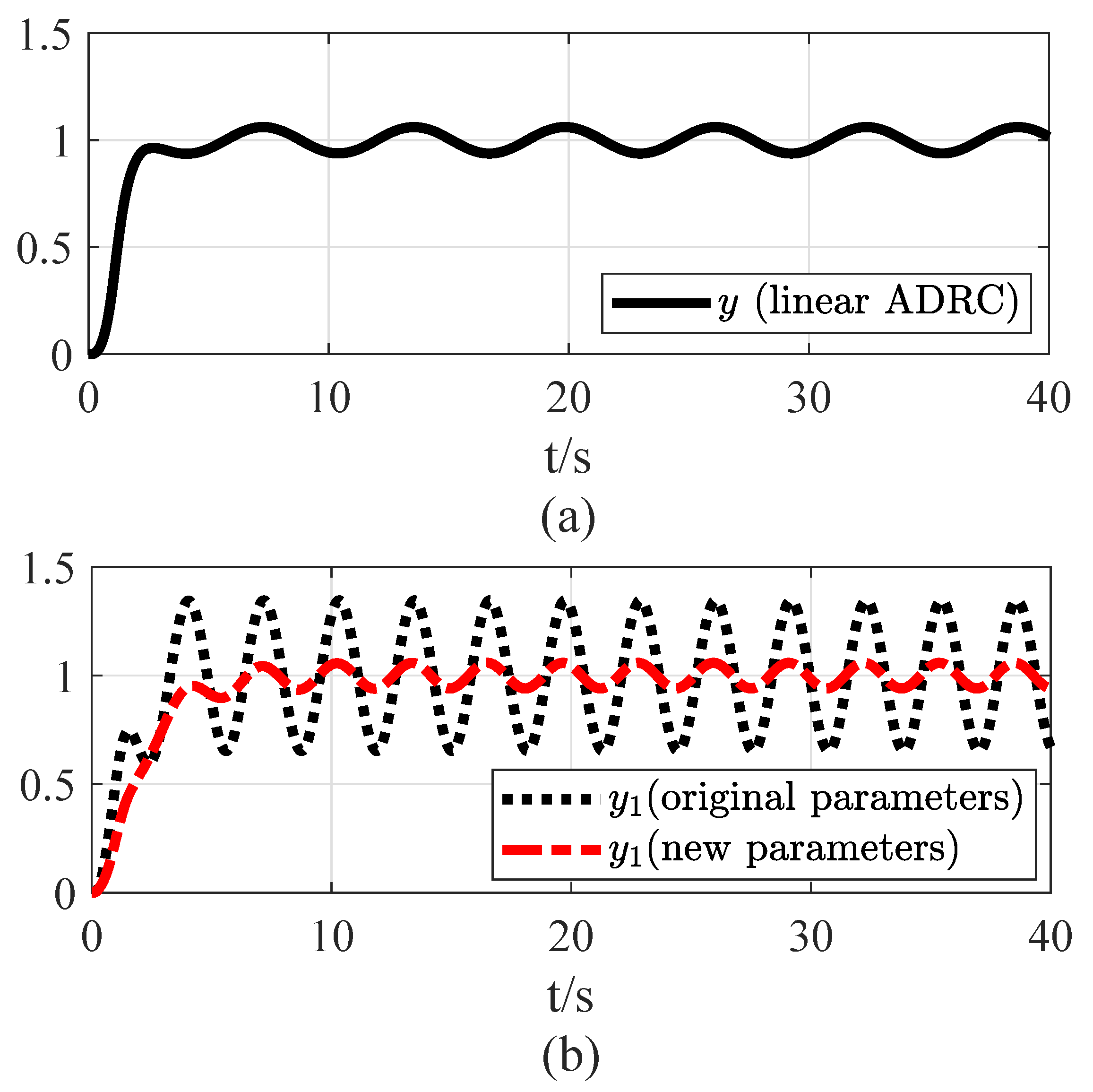
4.3. Control Performance of ADRC

For the overall ADRC parameter tuning, a linear ADRC is employed to validate the efficacy of the proposed parameter tuning rule. The program environment used above remains unchanged. The original system (1) is set as x ¨ 1 = F + b 0 u = μ 0 sin ( w 0 t ) + b 0 u , μ 0 = 1 , w 0 = 1 . The input is u and the reference value is v 0 = 1. According to the trial-and-error method, a set of linear ADRC parameters are obtained as follows: r 0 = 3 , β 01 = 30 , β 02 = 300 , β 03 = 1000 , b 0 = 1 , k p = 7 , k d = 12.25 . The simulation results of the original system under the linear ADRC method are shown in Figure 8a. When the original system is modified to x ¨ 1 = F 1 + b 01 u = A sin ( k w 0 t ) + b 01 u , A = 4 μ 0 , k = 2 . By (21), the new parameters are obtained as r n = 6 , β 010 = 60 , β 020 = 1200 , β 030 = 8000 , b 01 = 4 , k p = 14 , k d = 49 .
From Figure 8b, it is obvious that the control performance of ADRC is significantly improved for the transformed system. This means that the proposed parameter tuning rule for ADRC is effective.

5. Application

In this section, the ADRC method based on the proposed parameter tuning rule is applied to the intake pressure control of the flight test chamber system.

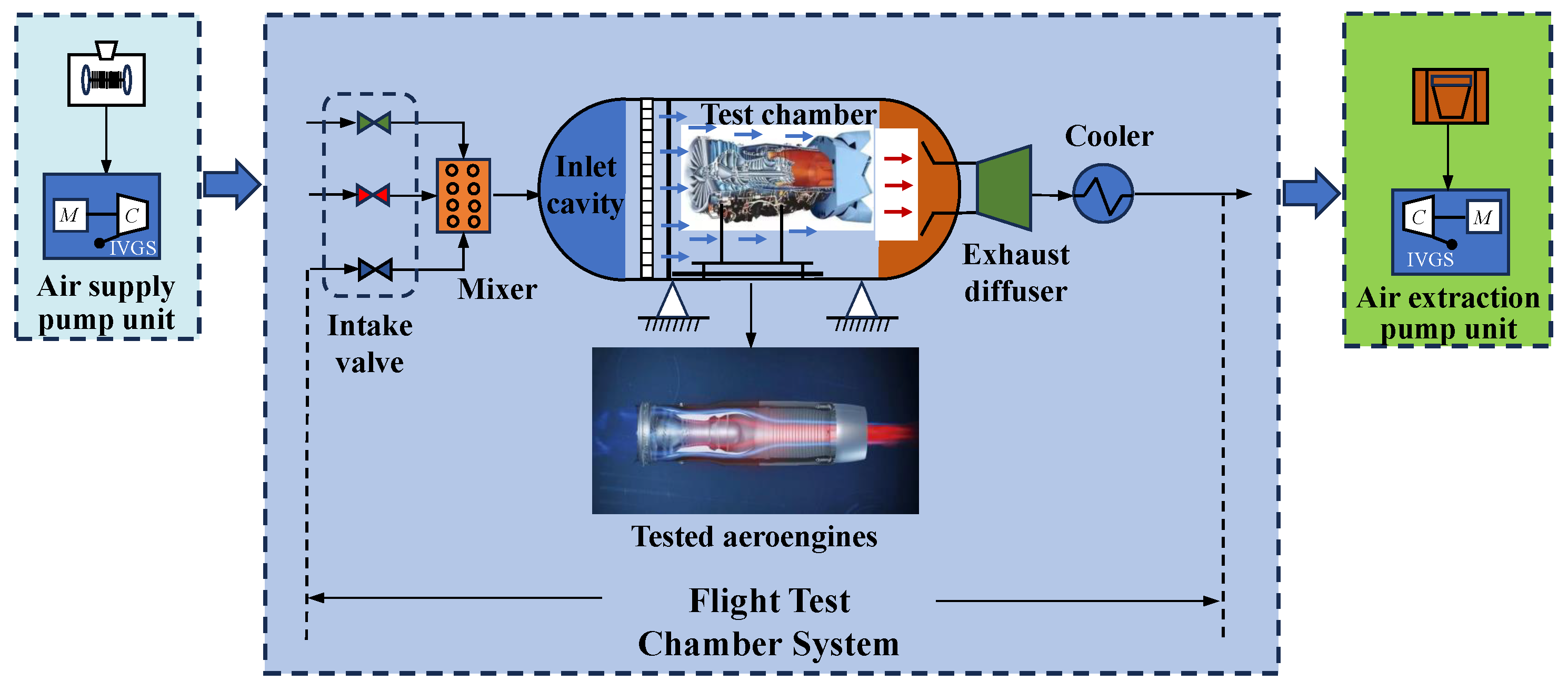
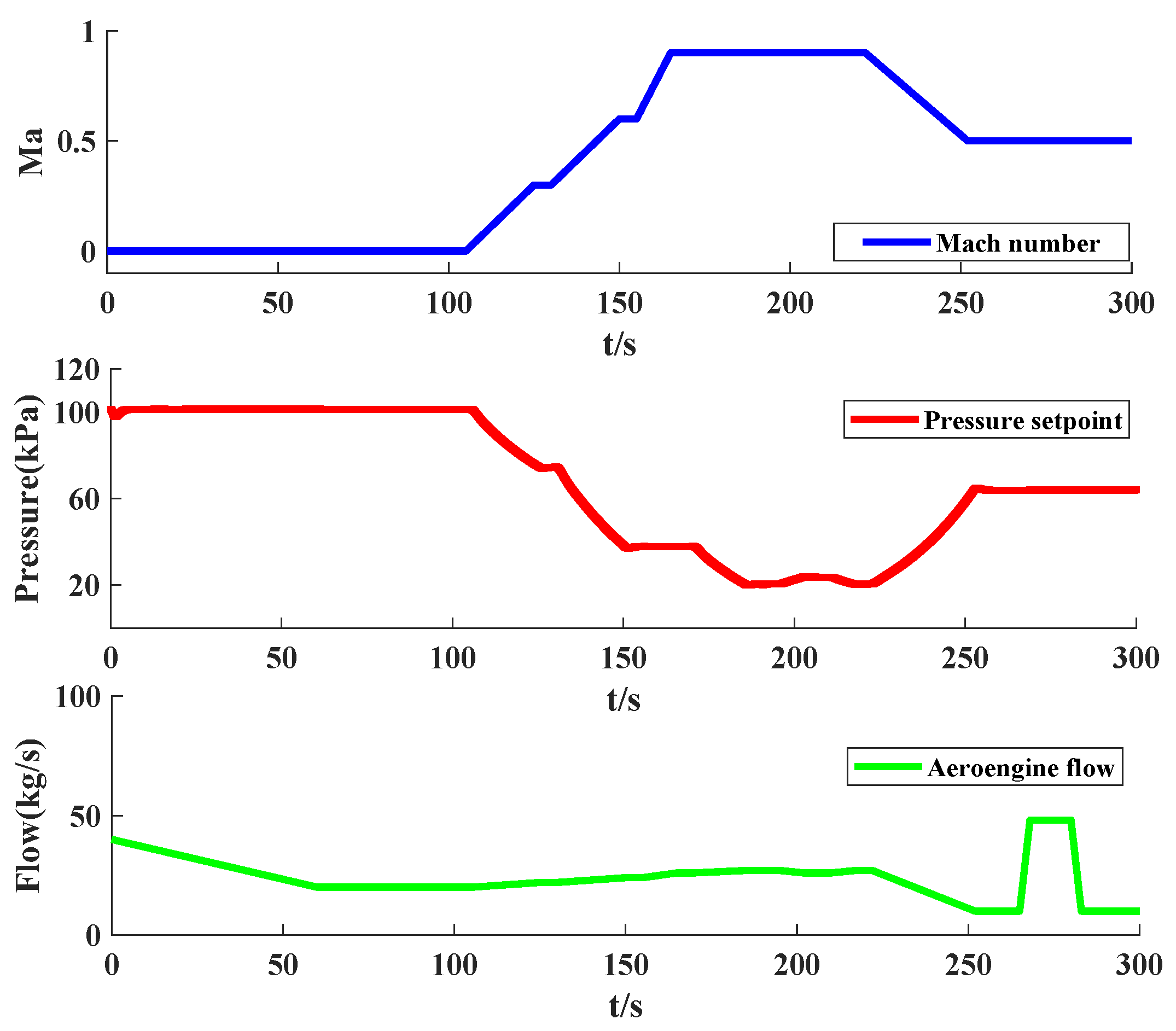
5.1. Introduction of the Flight Test Chamber System

The flight test chamber system, serving as a critical control component for establishing aeroengine flight conditions, comprises several essential elements including the intake valve, mixer, test chamber, exhaust diffuser, cooler, air supply pump unit and air extraction pump unit, with its structural diagram as shown in Figure 9.
The control principle of the flight test chamber system is to regulate the intake valve to control the intake pressure, enabling simulation of intake conditions in the inlet cavity, which constructs the aeroengine actual flight environment [32]. In practical aeroengine testing, particularly during transient operations, rapid airflow changes often lead to significant variations in environmental parameters and system characteristics. Traditional approaches utilizing fixed ADRC parameters or empirical tuning methods are insufficient to ensure control quality across diverse test conditions, often leading to system instability. To guarantee control quality, particularly during transient state, the proposed spatial–temporal scale transformation-based parameter tuning method provides an efficient and reliable strategy for adaptively adjusting ADRC parameters in response to system characteristic variations.

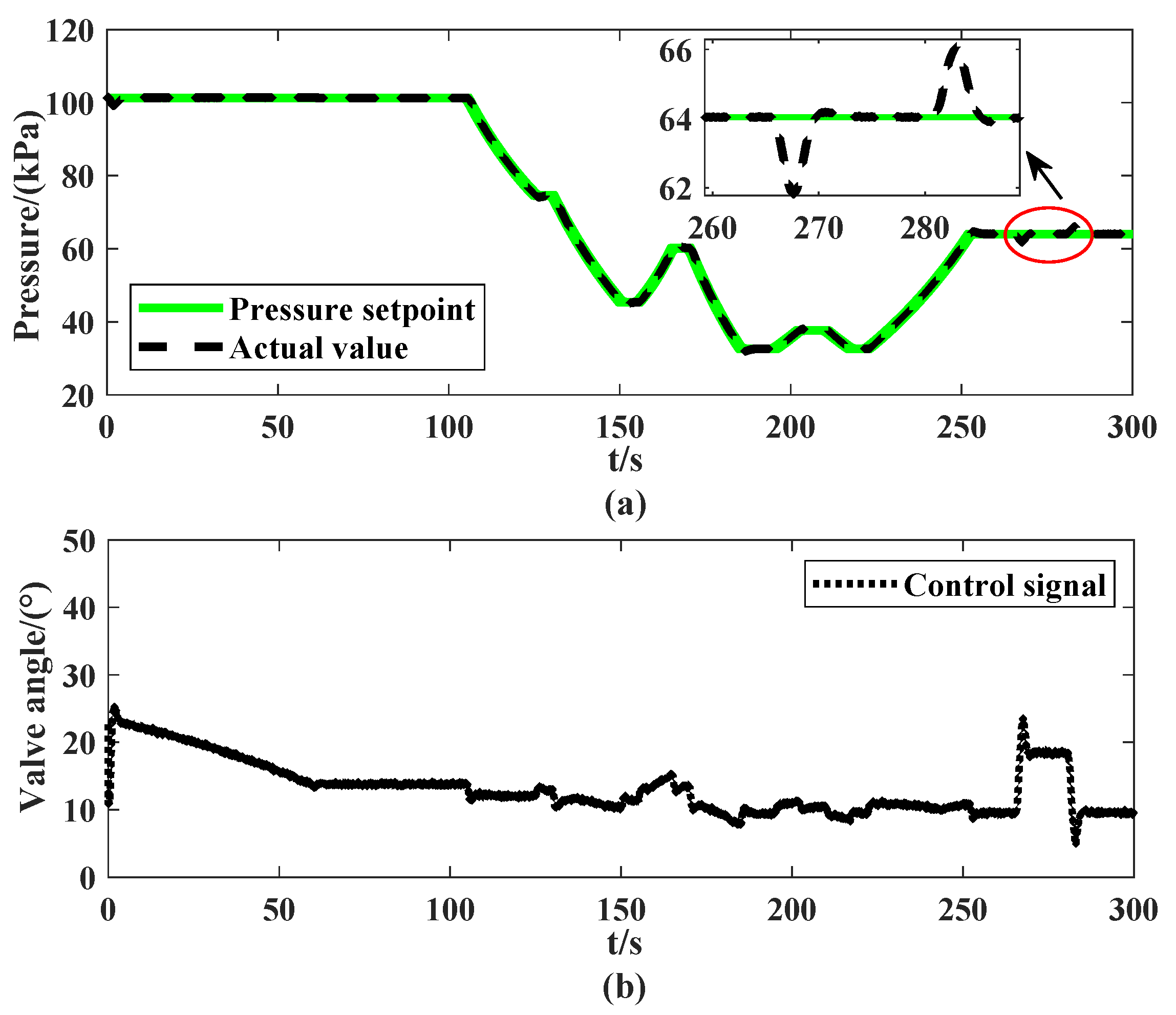
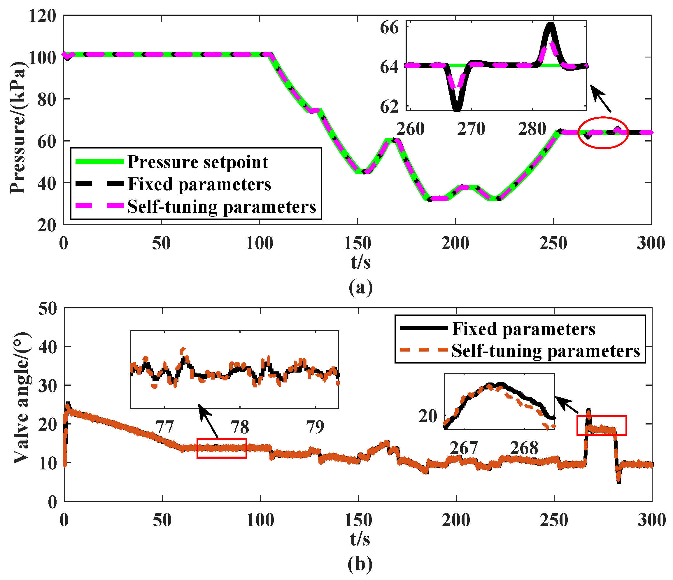
5.2. Test Results and Analysis

For the intake pressure control of the flight test chamber system, the frequency and amplitude characteristics of the measured pressure signal are obtained by analyzing extensive experimental data. The spatial–temporal scale transformation method is then applied to self-tune ADRC parameters, ensuring satisfactory control performance under different aeroengine test conditions. The test condition 1 of the aeroengine is established, as illustrated in Figure 10. The test variables include the flight Mach number, pressure setpoint and aeroengine flow. Meanwhile, under test condition 1, the corresponding spatial- and temporal-scale amplitude characteristic curves of the intake pressure signal are plotted, as can be seen in Figure 11.
Based on the trial-and-error method, a suitable set of ADRC control parameters for test condition 1 is obtained, with the parameters selected as follows: r 0 = 3000 , β 01 = 45 , β 02 = 675 , β 03 = 3375 , k p = 2.4 , k p = 1.44 . The results of the intake pressure control response and control signal are shown in Figure 12. Figure 12 demonstrates that the ADRC controller achieve precise intake pressure control in the flight test chamber system under the specified parameter configuration.
The aeroengine test conditions are changed to accommodate different testing requirements. By adjusting the flight Mach number, pressure setpoint and aeroengine flow, a new test condition (i.e., test condition 2) is established, as depicted in Figure 13. The ADRC parameters of test condition 1 are kept unchanged and directly applied to the intake pressure control of the flight test chamber system under test condition 2. The results of control performance are presented in Figure 14.
It is obvious, as shown in Figure 14, that when the ADRC parameters of test condition 1 are applied to the intake pressure control of the flight test chamber system under test condition 2, the control performance is seriously limited. Specifically, the maximum pressure error increases from nearly 0 kPa to 2.1 kPa, and the maximum convergence time reaches 8.0 s. Especially during the fast transient phase (i.e., 250∼300 s), when the aeroengine flow changes rapidly and dramatically, it causes large fluctuations in the controlled pressure and a long recovery time. This is caused by the changes in the test condition and the system characteristics, that is, the spatial and temporal scales (or the amplitude and frequency of the signal) change (see Figure 15). The control parameters of ADRC should also be adjusted accordingly to guarantee the control performance under the new operating conditions. Based on the proposed parameter tuning rule (21), the parameters of ADRC are adaptively adjusted. The tuning process of the three critical ADRC components (TD, ESO and feedback controller) are presented in Figure 16.
According to this ADRC self-tuning method, the intake pressure control results of the flight test chamber system are shown in Figure 17. As can be seen from Figure 17, when the fixed parameters of ADRC are adopted, the maximum pressure error is 2.0 kPa, while the maximum pressure error with the self-tuning parameters is only 0.9 kPa. Under test condition 2, compared to the performance with fixed ADRC parameters, the tuned parameters obtained by the proposed method effectively reduce fluctuations and convergence time during the fast transient phase (250∼300 s), while maintaining the control signal at a similar level for both parameter sets. The quantitative comparison is summarized in Table 1. Therefore, when the test conditions of the flight test chamber system change, tuning the ADRC parameters using the proposed method can significantly improve control performance.

6. Conclusions

This work proposed a parameter self-tuning method based on spatial–temporal scale transformations for ADRC to simplify ADRC tuning and enhance its control performance. By establishing a mapping relationship between the spatial–temporal scale and control parameters, this method enables us to systematically adjust ADRC parameters in accordance with variations in system dynamics, eliminating the need for re-identification or re-modeling. Numerical simulation results demonstrated that the proposed parameter tuning rule is effective for the parameter tuning of TD, ESO, and the overall ADRC. Additionally, test results showed that the proposed approach can significantly improve the control performace of the intake pressure system when the aeroengine test condition changes. These results show that the proposed method not only improves control robustness under rapidly changing conditions, but also enhances efficiency for multi-condition aeroengine tests by enabling scalable parameter reuse. Future work will include introducing the proposed parameter self-tuning method into other improved ADRC controllers.

Author Contributions

Conceptualization, Z.X. and H.Z.; methodology, Z.X.; software, Z.X.; validation, Z.X., Y.X., C.Z. and X.W.; formal analysis, X.W.; investigation, H.Z.; resources, H.Z.; data curation, Y.X.; writing—original draft preparation, Z.X., H.Z. and Y.X.; writing—review and editing, Z.X., H.Z., Y.X., C.Z., X.W. and F.H.; visualization, Z.X. and X.W.; supervision, H.Z. and F.H.; project administration, H.Z. and F.H.; funding acquisition, H.Z. All authors have read and agreed to the published version of the manuscript.

Funding

This work is supported by the National Natural Science Foundation of Fujian Province (Grant No. 2021J02008); in part by the the Project (Grant No.GJCZ-0303-2024-0005); and part of this work is also supported by the National Natural Science Foundation of China (Grant No. 62003088).

Data Availability Statement

Data are contained within the article.

Conflicts of Interest

Author Yunde Xie was employed by the company Huida Technology Development Co., Ltd. The remaining authors declare that the research was conducted in the absence of any commercial or financial relationships that could be construed as a potential conflict of interest.

References

  1. Afkhami, S.; Fouladi, N.; Fard, M.P. Experimental and numerical investigation of transient starting of pre-evacuated exhaust diffuser in high altitude ground test. Aerosp. Sci. Technol. 2023, 133, 108111. [Google Scholar] [CrossRef]
  2. Zhu, M.; Wang, X.; Zhang, S.; Dan, Z.; Pei, X.; Miao, K.; Jiang, Z. PI gain scheduling control for flight environment simulation system of altitude ground test facilities based on LMI pole assignment. J. Propuls. Technol. 2019, 40, 2587–2597. [Google Scholar]
  3. Chen, W.; Yang, J.; Guo, L.; Li, S. Disturbance-observer-based control and related methods—An overview. IEEE Trans. Ind. Electron. 2015, 63, 1083–1095. [Google Scholar] [CrossRef]
  4. McKercher, R.G.; Khouli, F.; Wall, A.S.; Larose, G.L. Modelling and control of an urban air mobility vehicle subject to empirically-developed urban airflow disturbances. Aerospace 2024, 11, 220. [Google Scholar] [CrossRef]
  5. Li, S.; Yang, J.; Iwasaki, M.; Chen, W.H. Hierarchical disturbance/uncertainty estimation and attenuation for integrated modeling and motion control: Overview and perspectives. IEEE/ASME Trans. Mechatron. 2025, 25, 1–15. [Google Scholar] [CrossRef]
  6. Han, J. From PID to active disturbance rejection control. IEEE Trans. Ind. Electron. 2009, 56, 900–906. [Google Scholar] [CrossRef]
  7. Gao, Z. Scaling and bandwidth-parameterization based controller tuning. In Proceedings of the ACC, Denver, CO, USA, 4–6 June 2003; pp. 4989–4996. [Google Scholar]
  8. Li, J.; Zhang, L.; Li, S.; Mao, Q.; Mao, Y. Active disturbance rejection control for piezoelectric smart structures: A review. Machines 2023, 11, 174. [Google Scholar] [CrossRef]
  9. Chen, S.; Chen, Z.; Zhao, Z.L. Parameter selection and performance analysis of linear disturbance observer based control for a class of nonlinear uncertain systems. IEEE Trans. Ind. Electron. 2021, 70, 11587–11597. [Google Scholar] [CrossRef]
  10. Guo, B.; Bacha, S.; Alamir, M.; Hably, A.; Boudinet, C. Generalized integrator-extended state observer with applications to grid-connected converters in the presence of disturbances. IEEE Trans. Control Syst. Technol. 2020, 29, 744–755. [Google Scholar] [CrossRef]
  11. Su, Z.g.; Sun, L.; Xue, W.; Lee, K.Y. A review on active disturbance rejection control of power generation systems: Fundamentals, tunings and practices. Control Eng. Pract. 2023, 141, 105716. [Google Scholar] [CrossRef]
  12. Li, S.; Lu, H.; Li, J.; Zheng, T.; He, Y. Fractional-order sliding mode controller based on ESO for a buck converter with mismatched disturbances: Design and experiments. IEEE Trans. Ind. Electron. 2025; in press. [Google Scholar] [CrossRef]
  13. Chen, S.; Xue, W.; Huang, Y.; Liu, P. On comparison between smith predictor and predictor observer based adrcs for nonlinear uncertain systems with output delay. In Proceedings of the ACC, Seattle, WA, USA, 24–26 May 2017; pp. 5083–5088. [Google Scholar]
  14. Hou, Q.; Zuo, Y.; Sun, J.; Lee, C.H.; Wang, Y.; Ding, S. Modified nonlinear active disturbance rejection control for PMSM speed regulation with frequency domain analysis. IEEE Trans. Power Electron. 2023, 38, 8126–8134. [Google Scholar] [CrossRef]
  15. Li, C.; Zhai, C.; Zhang, H.; Zheng, S. PSO-SMADRC for altitude test facility intake pressure environmental simulation system. Electron. Lett. 2024, 60, e13105. [Google Scholar]
  16. Wang, C.; Du, X.; Sun, X. Performance-seeking control of aero-propulsion system based on intelligent optimization and active disturbance rejection fusion controller. Aerospace 2023, 10, 151. [Google Scholar] [CrossRef]
  17. Xu, Z.; Zhang, H.; Zhai, C.; Qian, Q.; Wu, L. Fixed time active disturbance rejection compound decoupling control method for intake environment simulation system of altitude test facility. J. Propuls. Technol. 2024, 46, 239–252. [Google Scholar] [CrossRef]
  18. Li, C.; Zhang, H.; Gaoxi, X.; Zhai, C.; Dan, Z.; Wang, X. An efficient tracking differentiator based active disturbance rejection control for flight environment simulation system. Aerosp. Sci. Technol. 2024, 155, 109578. [Google Scholar] [CrossRef]
  19. Ran, M.; Li, J.; Xie, L. A new extended state observer for uncertain nonlinear systems. Automatica. 2021, 131, 109772. [Google Scholar] [CrossRef]
  20. Du, Y.; She, J.; Cao, W. Improving performance of disturbance rejection for nonlinear systems using improved equivalent-input-disturbance approach. IEEE Trans. Ind. Electron. 2023, 20, 941–952. [Google Scholar] [CrossRef]
  21. Zaragoza Prous, G.; Grustan-Gutierrez, E.; Felicetti, L. A decreasing horizon model predictive control for landing reusable launch vehicles. Aerospace 2025, 12, 111. [Google Scholar] [CrossRef]
  22. Chang, S.; Cao, J.; Pang, J.; Zhou, F.; Chen, W. Compensation control strategy for photoelectric stabilized platform based on disturbance observation. Aerosp. Sci. Technol. 2024, 145, 108909. [Google Scholar] [CrossRef]
  23. Li, J.; Xia, Y.; Qi, X.; Gao, Z. On the necessity, scheme, and basis of the linear–nonlinear switching in active disturbance rejection control. IEEE Trans. Ind. Electron. 2016, 64, 1425–1435. [Google Scholar] [CrossRef]
  24. Sun, L.; Xue, W.; Li, D.; Zhu, H.; Su, Z.g. Quantitative tuning of active disturbance rejection controller for FOPTD model with application to power plant control. IEEE Trans. Ind. Electron. 2021, 69, 805–815. [Google Scholar] [CrossRef]
  25. Yuan, D.; Ma, X.; Zeng, Q.; Qiu, X. Research on frequency-band characteristics and parameters configuration of linear active disturbance rejection control for second-order systems. Control Theory Appl. 2013, 30, 1630–1640. [Google Scholar]
  26. Liang, Q.; Wang, C.; Pan, J.; Wei, Y.; Yong, W. Parameter identification of b0 and parameter tuning law in linear active disturbance rejection control. Control Decis. 2015, 30, 1691–1695. [Google Scholar]
  27. Chen, Z.; Hao, Y.; Su, Z.; Sun, L. Data-driven iterative tuning based active disturbance rejection control for FOPTD model. ISA Trans. 2022, 128, 593–605. [Google Scholar] [CrossRef]
  28. Li, S.; Zhang, S.; Liu, Y.; Zhou, S. Parameter-tuning in active disturbance rejection controller using time scale. Control Theory Appl. 2012, 29, 125–129. [Google Scholar]
  29. Zhang, H.; Xie, Y.; Wang, J.; Dan, Z.; Guo, W. Parameter tuning algorithm for levant’s differentiator and its application in flight environment simulation control system. Control Theory Appl. 2023, 40, 1831–1838. [Google Scholar]
  30. Wang, J.; Zhang, H.; Dan, Z.; Zhang, S.; Xiao, G.; Zhai, C. A practical parameter tuning algorithm for super-twisting algorithm-based differentiator and its application in altitude ground test facility. Trans. Inst. Meas. Control 2024, 47, 610–620. [Google Scholar] [CrossRef]
  31. Ran, M.; Wang, Q.; Dong, C. Active disturbance rejection control for uncertain nonaffine-in-control nonlinear systems. IEEE Trans. Autom. Control 2016, 62, 5830–5836. [Google Scholar] [CrossRef]
  32. Liu, J.; Wang, X.; Liu, X.; Zhu, M.; Pei, X.; Dan, Z.; Zhang, S. μ-Synthesis-based robust L1 adaptive control for aeropropulsion system test facility. Aerosp. Sci. Technol. 2023, 140, 108457. [Google Scholar] [CrossRef]
Figure 1. Structure of ADRC for the flight test chamber system.
Aerospace 12 00465 g001
Figure 2. Control parameters of ADRC for the flight test chamber system.
Aerospace 12 00465 g002
Figure 3. Parameter tuning process of ADRC for the flight test chamber system.
Aerospace 12 00465 g003
Figure 4. Performances of TD under original signal v 0 : (a) signal tracking; (b) differentiation acquisition.
Aerospace 12 00465 g004
Figure 5. Performances of TD under new signal v n : (a) signal tracking; (b) differentiation acquisition.
Aerospace 12 00465 g005
Figure 6. Performances of ESO under F: (a) system output estimation; (b) total disturbance estimation.
Aerospace 12 00465 g006
Figure 7. Performances of ESO under F 1 : (a) system output estimation; (b) total disturbance estimation.
Aerospace 12 00465 g007
Figure 8. Performances of linear ADRC: (a) control response of original system; (b) control response of transformed system under different parameters.
Aerospace 12 00465 g008
Figure 9. Structural diagram of the flight test chamber system.
Aerospace 12 00465 g009
Figure 10. Test condition 1 of the flight test chamber system.
Aerospace 12 00465 g010
Figure 11. Spatial–temporal-scale amplitude characteristic curves of the intake pressure signal.
Aerospace 12 00465 g011
Figure 12. Results of the intake pressure control response and control signal: (a) control response; (b) control signal.
Aerospace 12 00465 g012
Figure 13. Test condition 2 of the flight test chamber system.
Aerospace 12 00465 g013
Figure 14. Results of the intake pressure control response and control signal: (a) control response; (b) control signal.
Aerospace 12 00465 g014
Figure 15. Spatial–temporal-scale amplitude characteristic curves of the intake pressure signal.
Aerospace 12 00465 g015
Figure 16. Parameter tuning process based on the proposed space/time scale transformation.
Aerospace 12 00465 g016
Figure 17. Results of the intake pressure control response and control signal: (a) control response; (b) control signal.
Aerospace 12 00465 g017
Table 1. The quantitative comparison of fixed parameters and the proposed method.
PerformanceApproach250∼300 sPercentage Improvement
Maximum pressure
error (kPa)
Fixed parameters2.1
Self-tuning parameters0.9 57 %
Maximum convergence
time (s)
Fixed parameters8.0
Self-tuning parameters4.8 40 %
Disclaimer/Publisher’s Note: The statements, opinions and data contained in all publications are solely those of the individual author(s) and contributor(s) and not of MDPI and/or the editor(s). MDPI and/or the editor(s) disclaim responsibility for any injury to people or property resulting from any ideas, methods, instructions or products referred to in the content.

