Abstract
With the rapid development of both commercial and general aviation, the frequency assignment problem for aviation navigation stations has become increasingly important. This paper presents a general algorithm for frequency assignment at individual aviation navigation stations. Subsequently, a frequency assignment model for multiple civil aviation navigation stations is established to address large-scale frequency allocation challenges. To overcome the limitations of traditional multi-objective genetic algorithms, such as slow convergence speed and susceptibility to local optima, this study proposes several improved algorithms, including the multi-objective genetic algorithm with randomly assigned weights, the multi-objective genetic local search algorithm, and an improved multi-objective genetic local search algorithm, while optimizing key algorithm parameters. The problem involves multiple objectives, including minimizing interference in frequency assignment and reducing the total number of assigned frequencies. Experimental results demonstrate that the proposed improved multi-objective genetic algorithms—especially IMOGLSA-II—effectively address the frequency assignment problem for aviation navigation stations, achieving notable improvements in solution quality, convergence speed, and stability compared with other multi-objective genetic algorithms. In particular, although the time complexity of the proposed algorithm is slightly higher due to the incorporation of local search mechanisms, it exhibits clear advantages in reducing parameter sensitivity, simplifying algorithm structure, and enhancing engineering applicability. These characteristics make the proposed method not only well-suited to the static and constrained nature of aviation frequency assignment, but also more practical and effective than other mainstream multi-objective optimization algorithms in similar engineering scenarios. Furthermore, the proposed method offers a reliable approach that can be extended to other static frequency assignment problems and broader classes of multi-objective optimization tasks.
1. Introduction
Aeronautical radio navigation is a crucial component of the air navigation system established by the International Civil Aviation Organization (ICAO), providing essential flight guidance information to ensure that aircraft can navigate safely and accurately along designated routes and arrive at their destinations on time. According to data from the Civil Aviation Administration of China (CAAC), the number of civil aviation airports in China has been steadily increasing, reaching 250 by 2020. Moreover, plans have been made to construct an additional 136 airports by 2025. The number of registered civil aircraft in China also grew significantly, rising from 2950 in 2015 to 4244 in 2022, representing an approximate 44% increase over 7 years. This substantial growth in the number of aircraft has intensified the demand for navigation frequencies, posing considerable challenges for frequency assignment in both international and domestic civil aviation radio management. Enhancing frequency utilization efficiency and strengthening frequency resource management and allocation have become urgent problems that need to be addressed in civil aviation spectrum management.
Based on different frequency assignment strategies, the Frequency Assignment Problem (FAP) is generally classified into static frequency assignment and dynamic frequency assignment [1]. Static frequency assignment refers to a frequency management strategy in which limited frequency resources are pre-assigned to different radio stations within a specific time and space framework, and these assigned frequencies remain unchanged for a certain period. This method is suitable for scenarios where frequency assignment requirements do not frequently change. Dynamic frequency assignment, on the other hand, involves real-time adjustment and optimization of frequency resources according to actual communication demands and electromagnetic environmental changes [2]. This approach is more applicable to environments where communication requirements and electromagnetic threats fluctuate dynamically. Currently, the frequency assignment of civil aviation navigation stations falls under static frequency assignment.
Although frequency assignment has been widely studied and applied in various fields, most existing research has focused on military applications [3], mobile communications, and broadcasting stations. However, research on civil aviation navigation station frequency management, particularly under conditions of limited frequency resources and increasing frequency interference, remains relatively scarce.
In 2005, the Federal Aviation Administration (FAA) published the Spectrum Management Regulations and Procedures Manual [4], detailing frequency assignment methods for Very High Frequency (VHF) Omnidirectional Range (VOR), Distance Measuring Equipment (DME), and Instrument Landing System (ILS) systems. This manual emphasizes the use of appropriate spatial and frequency separations to ensure efficient frequency allocation, minimizing resource waste and harmful interference. In 2010, Kamali discussed the problem of frequency exhaustion in European VHF civil radio networks and proposed reducing channel protection spacing to increase the number of available frequencies [5], effectively addressing frequency scarcity. In 2015, the International Telecommunication Union (ITU) released the National Spectrum Management Handbook [6], which outlined technical methods to facilitate frequency coordination, including frequency separation and spatial separation. The handbook also provided general steps for assigning frequencies to individual stations and introduced metrics for measuring frequency utilization efficiency. More recently, in 2022, ICAO released the Civil Aviation Radio Spectrum Requirements Manual [7], which introduced electromagnetic compatibility calculation methods for civil aviation navigation equipment. The manual established the relationship between radio propagation losses and protection distances for navigation devices.
In summary, while frequency assignment has been extensively studied in multiple domains, including military applications, mobile communications, and broadcasting, research specifically focusing on civil aviation navigation stations remains insufficient, especially in the context of limited frequency resources and increasing interference challenges. This study aims to build upon frequency assignment research from other fields and to develop models and algorithms suitable for civil aviation navigation station frequency assignment.
The remainder of this paper is structured as follows:
Section 2: Frequency Assignment Model, introduces a multi-objective frequency assignment model tailored for civil aviation navigation stations.
Section 3: Multi-Objective Genetic Algorithm, presents traditional multi-objective genetic algorithms, the multi-objective genetic algorithm with randomly assigned weights, and the multi-objective genetic local search algorithm.
Section 4: Improved Multi-Objective Genetic Algorithm, proposes an improved multi-objective genetic algorithm based on multi-objective optimization theory.
Section 5: Results and Conclusion, discusses experimental results and provides the conclusions of this study.
For clarity, the main acronyms used throughout the paper are summarized in Table 1.

Table 1.
List of Acronyms and Their Descriptions.
2. Frequency Assignment Model
In the field of civil aviation, radio navigation systems primarily include the Instrument Landing System (ILS), Very High Frequency Omnidirectional Range (VOR), and Distance Measuring Equipment (DME). Within these systems, the two main components of ILS—the localizer (LOC) and the glide slope (GS)—operate in the very high frequency (VHF) band (108.10–111.95 MHz) and the ultra-high frequency (UHF) band (329.15–335 MHz), respectively. Similarly, the VOR system also operates in the VHF band, while DME utilizes the L-band (962–1213 MHz) for signal transmission [8].
According to the National Spectrum Management Handbook issued by the International Telecommunication Union (ITU) [6], key technical methods for optimizing frequency coordination include frequency separation and spatial separation. These methods are applicable to the general frequency assignment procedures for radio stations in China, as illustrated in Figure 1.
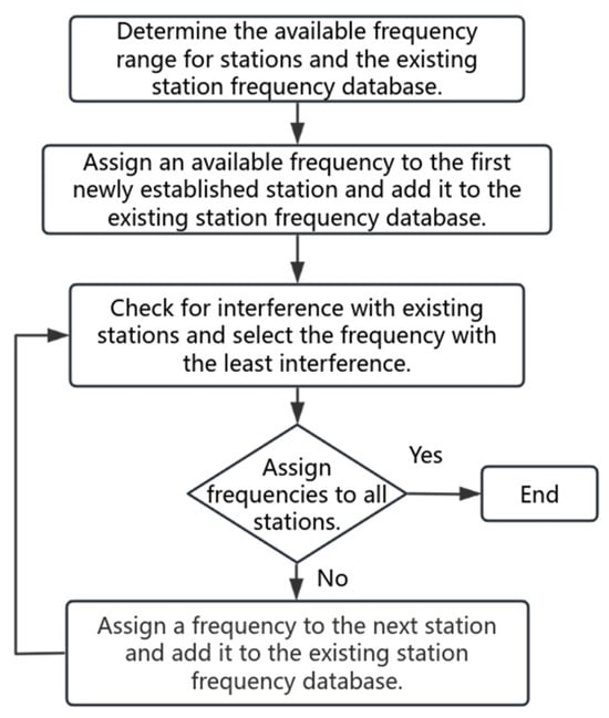
Figure 1.
General algorithm for frequency assignment of radio stations.
As shown in Figure 1, the general algorithm is not well-suited for large-scale frequency assignment in multiple stations. It suffers from low assignment efficiency and suboptimal frequency utilization. Therefore, to address this issue, a frequency assignment model suitable for multi-station scenarios has been developed.
There are various mathematical models for solving the Frequency Assignment Problem (FAP) [3]. The most commonly used approaches include:
- Optimization methods based on objective function optimization;
- Methods based on graph coloring theory;
- Grid-based frequency assignment methods using linear algebra techniques.
Currently, objective function optimization methods are widely applied in military frequency assignments. This study also adopts an objective function-based mathematical model to optimize frequency assignment in civil aviation navigation. The optimization objectives for frequency assignment can be categorized into several types, with the most commonly used ones including [9]:
- Minimum Order Frequency Assignment Problem (MO-FAP);
- Minimum Span Frequency Assignment Problem (MS-FAP);
- Minimum Blocking Frequency Assignment Problem (MB-FAP);
- Minimum Interference Frequency Assignment Problem (MI-FAP).
To enhance frequency utilization efficiency and ensure stable and continuous navigation services, this study focuses on optimizing two primary objectives:
- Minimum Order Frequency Assignment (MO-FAP): The objective of MO-FAP is to ensure that frequency assignment avoids any undesirable interference while minimizing the total number of assigned frequencies;
- Minimum Interference Frequency Assignment (MI-FAP): MI-FAP focuses on minimizing the weighted sum of all interference (i.e., penalty values) while ensuring that available frequency resources are efficiently utilized.
By optimizing these two objectives, the proposed model ensures efficient allocation of frequency resources while minimizing interference, ultimately improving frequency utilization efficiency and enhancing the operational quality of aviation navigation systems.
2.1. Interference Constraints
In frequency assignment problems, interference constraints are generally categorized into co-channel interference constraints, adjacent-channel interference constraints, and intermodulation interference constraints, with third-order intermodulation interference being the primary concern in the latter category [10].
To ensure the practical applicability of the proposed algorithm, this study incorporates multiple interference constraints, including:
- Interference between proposed navigation stations and existing navigation stations;
- Interference among proposed navigation stations;
- Frequency pairing interference constraints among VOR, LOC, and DME systems.
A crucial aspect to consider is that frequency pairing constraints must be accounted for regardless of whether a proposed VOR or LOC station requires a DME station. Based on the spectrum management regulations established by the Federal Aviation Administration (FAA), this study summarizes the interference constraint conditions and calculates the total interference count for each type of interference.
2.1.1. Co-Channel Interference Constraints
Co-channel interference constraints refer to restrictions placed on the use of the same frequency within radio stations to prevent interference between different transmitters [11]. In the spectrum management regulations outlined by the Federal Aviation Administration (FAA), Appendix 3 specifies the minimum protection distance (D1) required between two co-frequency VOR or LOC stations based on their power differences [4]. Additionally, it defines the minimum protection distance (D2) between two paired DME stations. Here, the first adjacent frequency of a DME station refers to the DME response frequency.
If the geographical separation between two stations is less than the minimum protection distance, it is considered that potential interference may occur between them. The total number of interference cases is determined using the following calculation:
- Calculation of Co-Channel Interference Between VOR or LOC Stations:
- 2.
- Calculation of Interference Between Paired DME Stations:
- 3.
- Total Number of Co-Channel Interference Cases:
2.1.2. Adjacent-Channel Interference Constraints
Adjacent-channel interference constraints are established to prevent mutual interference between signals operating on adjacent or nearby frequency channels [11]. These constraints ensure that assigned frequencies are spaced appropriately to minimize signal degradation and maintain navigation accuracy.
In the frequency assignment process for civil aviation VOR navigation stations, the following adjacent-channel interference cases must be considered:
- First adjacent-channel and second adjacent-channel interference between two VOR stations;
- First adjacent-channel interference between a VOR station and a LOC station.
In the frequency assignment process for LOC navigation stations, the following adjacent-channel interference cases must be considered:
- First adjacent-channel and second adjacent-channel interference between two LOC stations;
- First adjacent-channel interference between a VOR station and a LOC station.
Appendix 3 of the Federal Aviation Administration (FAA) Spectrum Management Regulations [4] specifies the minimum protection distances between stations based on power differences as follows:
- Minimum protection distance D3 between two first-adjacent frequency VOR stations (or two first-adjacent frequency LOC stations);
- Minimum protection distance D4 between two second-adjacent frequency VOR stations (or two second-adjacent frequency LOC stations);
- Minimum protection distance D5 between a VOR station and a LOC station operating on first-adjacent frequencies;
- Minimum protection distance D6 for the first-adjacent frequency of a DME station paired with a VOR (or LOC) station. Here, the first-adjacent frequency of a DME station refers to the DME response frequency.
As with co-channel interference, if the geographical separation between two stations is less than the corresponding minimum protection distance, it is considered that potential interference may occur. The total number of adjacent-channel interference cases is determined using the following calculation:
- Calculation of Adjacent-Channel Interference Between VOR (or LOC) Stations:
- 2.
- Calculation of Adjacent-Channel Interference Between VOR and LOC Stations:
- 3.
- Calculation of Adjacent-Channel Interference Between Paired DME Stations:
- 4.
- Total Number of Adjacent-Channel Interference Cases:
2.1.3. Third-Order Intermodulation Interference Constraints
Intermodulation interference occurs when the frequencies assigned to two stations undergo nonlinear interactions, resulting in the generation of new frequencies [12]. If these newly generated frequencies coincide with the operating frequencies of the station itself or neighboring stations, interference is introduced. Intermodulation interference can be classified into different orders, including second-order, third-order, and higher-order intermodulation interference. Among these, third-order intermodulation interference is the most severe. According to Appendix 3 of the FAA Spectrum Management Regulations [4], the maximum protection distances for intermodulation interference are specified as follows: maximum protection distance of 406 nautical miles between two VOR stations; maximum protection distance of 157 nautical miles between two LOC stations.
- Type I Third-Order Intermodulation Interference:
- 2.
- Type II Third-Order Intermodulation Interference:
- 3.
- Total Number of Third-Order Intermodulation Interference Cases:
2.1.4. Interference Constraints Between GS Stations
Although the protection range of LOC stations has already been designed to mitigate interference between GS (Glide Slope) stations, it is still necessary to prevent adjacent-frequency GS stations within the maximum protection range of 157 nautical miles between two LOC stations. This additional constraint helps further reduce potential interference between GS stations and ensures stable operation of the Instrument Landing System (ILS).
where: represent the GS (Glide Slope) frequencies paired with the ith proposed LOC station and the jth LOC station, respectively. = 3 indicates that interference occurs between two stations. = 0 indicates that no interference is detected.
From Equations (3), (7), (10), and (11), the total number of interference cases is the sum of the interference counts from co-channel interference, adjacent-channel interference, third-order intermodulation interference, and GS station interference:
2.2. Frequency Reuse
Frequency reuse is widely recognized as an effective approach to enhancing the utilization of frequency resources. To achieve the minimum order frequency assignment objective in this study, the Frequency Reuse Factor (FRF) is introduced [13].
The Frequency Reuse Factor is commonly used to quantify the extent to which the same frequency can be reused within a given area. It serves as a key metric for evaluating spectrum utilization efficiency. In practical applications, a higher Frequency Reuse Factor indicates that the same frequency can be reassigned multiple times within a specific region, thereby accommodating a greater number of navigation stations. This ultimately increases system capacity and optimizes frequency resource utilization.
The frequency reuse factor in this study is defined as follows:
where: t represents the station type and denotes the reuse count of the pth assigned frequency for this station type. q represents the total number of assigned frequencies for this station type. A larger value indicates that fewer distinct frequencies are used, implying a higher frequency reuse efficiency.
This study employs a mathematical model based on objective function optimization. By using the weighted sum method, the multi-objective optimization problem can be transformed into the following form:
where: , satisfying . The weight coefficient reflects the importance of each objective function. By selecting different weight combinations, various Pareto-optimal solutions can be obtained. The weighted sum method is one of the simplest and most effective classical approaches for solving multi-objective optimization problems [14]. Moreover, for convex Pareto-optimal frontiers, this method can efficiently find Pareto-optimal solutions.
According to Equations (12) and (13), the objective function in this study is defined as:
To prevent the formula from becoming invalid when I = 0, a positive constant A is introduced. and represent the weights of the two objective functions, satisfying and .
3. Multi-Objective Genetic Algorithm
Frequency assignment algorithms play a critical role in the management and optimization of radio networks. Their primary function is to efficiently allocate limited frequency resources to different radio equipment, ensuring the effective coexistence of stations within the network while maximizing frequency utilization efficiency. Frequency assignment algorithms can be broadly classified into deterministic algorithms and heuristic algorithms [15].
In the early stages of algorithm research, deterministic algorithms were widely used due to their simple structure and ease of implementation, particularly in scenarios where computational power and processing capabilities were limited. These algorithms provided effective solutions for frequency assignment problems. However, as system complexity increased, the limitations of deterministic algorithms became apparent, shifting the focus toward handling large-scale and complex systems [16]. To address these challenges, optimization algorithms emerged, including ant colony optimization (ACO), genetic algorithms (GA), tabu search (TS), simulated annealing (SA), and particle swarm optimization (PSO), among others.
In 1967, Rosenberg considered using genetic search algorithms to solve multi-objective optimization problems, introducing genetic algorithm (GA) concepts into multi-objective optimization, thereby pioneering research in the application of genetic algorithms to multi-objective optimization problems.
In the frequency assignment method for aviation navigation stations proposed in this study, which is based on objective function optimization, it is necessary to balance two primary objectives: minimizing interference in frequency assignment and minimizing the total number of assigned frequencies.
Genetic algorithms offer significant advantages in handling multi-objective optimization problems, as they can consider multiple objectives simultaneously within a unified computational framework. By designing an appropriate fitness function, the minimization of interference and frequency count can be integrated into a single algorithm, allowing the trade-off between these two optimization objectives to be effectively managed. This enables the discovery of an optimal or near-optimal solution that meets practical requirements. Specifically, the fitness function is weighted based on the severity of electromagnetic interference and the number of assigned frequencies, assigning appropriate weight coefficients to balance the relative importance of different optimization objectives. Therefore, this study adopts genetic algorithms to compute the proposed frequency assignment model.
3.1. Traditional Multi-Objective Genetic Algorithm
3.1.1. Chromosome Representation and Encoding
In genetic algorithms (GA), encoding methods typically fall into two common types: symbolic encoding and binary encoding. The choice of encoding method affects the representation capability and computational efficiency of the algorithm.
According to the overview of aviation navigation station systems in Section 2, the frequencies used in aviation navigation stations are discrete frequency points within their respective available bands, and the spacing between these frequency points is not uniform. Therefore, to better accommodate this characteristic, this study adopts the symbolic encoding method for frequency assignment [17].
For example, when assigning frequencies to five VOR-H navigation stations, an individual in the genetic algorithm consists of five genes, with each gene representing the frequency assignment result for a navigation station. In other words, these five genes together form a complete frequency assignment scheme, referred to as a frequency assignment group. As shown in Figure 2, the encoding method maps the frequency requirement of each navigation station to a gene value, allowing the individual to concisely represent the entire frequency assignment scheme.
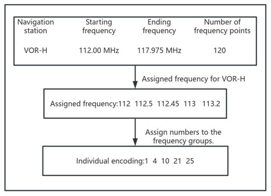
Figure 2.
Encoding diagram.
3.1.2. Population Initialization
In traditional genetic algorithms, population initialization is typically performed using a random initialization method. This process aims to generate a set of candidate solutions (individuals) through random number generation, forming a diverse initial population. Specifically, the gene value range for each candidate solution is determined based on the problem constraints, and random initialization generates individuals within this range, ensuring population diversity. This method not only provides broad coverage of the solution space but also enhances the algorithm’s global search capability in the initial stage, laying a strong foundation for subsequent genetic operations such as selection, crossover, and mutation [18]. The detailed process is illustrated in Figure 3.
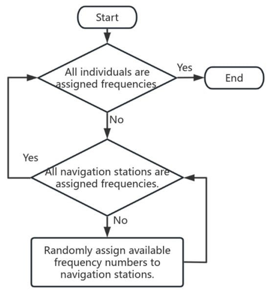
Figure 3.
Population initialization flowchart.
3.1.3. Fitness Function
After population initialization is completed, the next step is to evaluate the fitness of each individual. The fitness function serves as the core criterion for this evaluation process. Based on the frequency assignment model described in Section 2, the fitness function is designed as follows:
where: i represents an individual.
The flowchart of population fitness evaluation is illustrated in Figure 4:
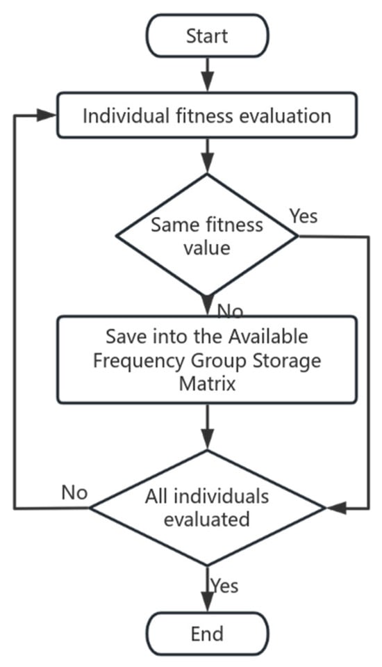
Figure 4.
Population fitness evaluation flowchart.
3.1.4. Selection Operation
This study adopts the Roulette Wheel Selection method, which is named after the classic roulette game [19]. In this method, each individual is assigned a selection probability, which is proportional to its fitness value. The higher the fitness of an individual, the greater the probability of being selected. This mechanism ensures that fitter individuals are more likely to be passed on to the next generation, while less fit individuals are gradually eliminated.
- Compute total fitness:
- 2.
- Determine selection probability:
- 3.
- Select individuals: Generate a random number within the range (0, 1). Based on this random number, simulate a roulette wheel spin according to the fitness proportion of each individual. The individual whose fitness range the random number falls into is selected. Repeat this process until the required number of individuals for reproduction is chosen. In this study, the number of selected individuals is equal to the population size M.
The flowchart of the selection operation is illustrated in Figure 5.
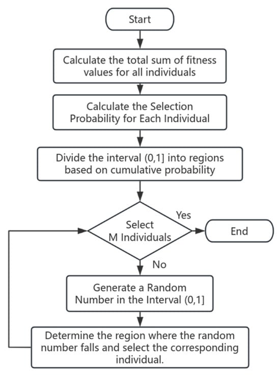
Figure 5.
Selection operation flowchart.
3.1.5. Crossover Operation
This study adopts the single-point crossover method, which is widely used due to its simplicity and ease of implementation. This method effectively recombines genetic information from parent individuals by exchanging gene segments to generate offspring with new characteristics. The key feature of single-point crossover is that a random crossover point is selected within the gene sequence. The genetic material of the two parent individuals is then split at this point into two segments, and the segments after the crossover point are swapped, forming a new gene combination for the offspring [20]. Based on empirical studies, a reasonable range for the crossover probability is between 0.4 and 0.99 [21].
Specific Steps: Generate a random number within the interval (0,1) and compare it with the crossover probability Pc. If the random number is less than , perform the crossover operation by randomly selecting a crossover point on the parent chromosomes, which corresponds to a specific gene position in the chromosome. The gene segments after the crossover point are then swapped between the two parents to create new offspring. If the random number is greater than or equal to , no crossover occurs, and the parent individuals are directly retained in the next generation.
The diagram of the crossover operation is illustrated in Figure 6.
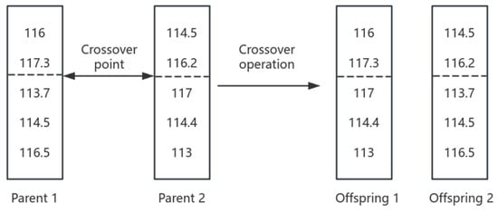
Figure 6.
Crossover operation diagram.
3.1.6. Mutation Operation
The key parameter in the mutation operation is the mutation probability , which represents the probability of a gene undergoing mutation within an individual. The setting of requires careful consideration. If is set too high, a large number of genes will mutate, generating a significant number of new individuals. However, this may disrupt optimal genetic patterns, negatively impacting the algorithm’s performance. Conversely, if is set too low, the ability to generate new solutions through mutation is weakened, making it difficult to maintain population diversity. This can lead to premature convergence at a local optimum, preventing the algorithm from fully exploring the solution space. Based on empirical studies, the typical range for is 0.01 to 0.1.
It is important to note that the new gene randomly selected during mutation must come from the civil aviation navigation station frequency database provided in Reference [22]. This ensures that the mutated solutions are not only genetically diverse but also practically feasible for real-world applications.
The diagram of the mutation operation is illustrated in Figure 7.
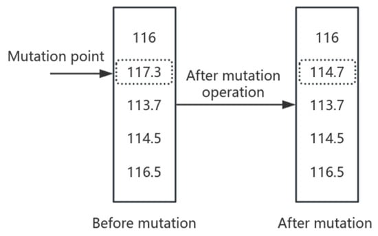
Figure 7.
Mutation operation diagram.
3.2. Randomly Assigned Weights
In traditional multi-objective optimization methods, the weight distribution among different objectives is typically fixed. This fixed weighting strategy imposes a certain level of rigidity on the algorithm, causing its search direction to remain unchanged throughout the iterative process. Consequently, regardless of the solution encountered, the optimization process always progresses in the same direction, making it incapable of dynamically adjusting based on the distribution of solutions or the needs of different objectives. This limitation may make it difficult for the algorithm to achieve a balanced trade-off between multiple objectives, particularly in cases where objective conflicts arise or when weight allocation is inappropriate, potentially leading to a final solution that deviates from the desired global optimum [23].
In multi-objective optimization problems, the way weights are assigned to different objectives directly affects the convergence path of the algorithm and the quality of the final solution. Fixed weight allocation means that the importance ratio of each objective is predetermined at the beginning of the optimization process and remains unchanged throughout the search, limiting the algorithm’s ability to dynamically adjust the trade-offs among multiple objectives.
Figure 8 illustrates the search directions for different fixed weight values.
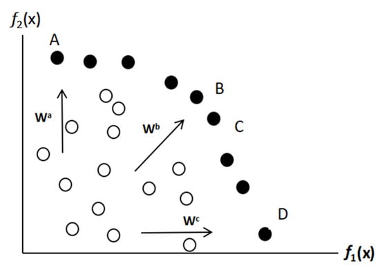
Figure 8.
Search directions for different fixed weight values in multi-objective functions.
In the figure, represent three different fixed weight values. For example, when searching with = (0.5, 0.5), the algorithm prioritizes finding the optimal solutions for objectives B and C, making it easier to obtain solutions that satisfy this specific weight distribution. However, solutions A and D cannot be found using a fixed weight approach, as they require adjustments in weight distribution and changes in search direction to be discovered.
To address this limitation, this study introduces a dynamic weight adjustment strategy, allowing the algorithm to adaptively adjust the weight proportions of different objectives based on actual requirements during the search process. As a result, the algorithm can not only dynamically change its search direction and expand the solution space exploration range, but also flexibly identify diverse solutions under different weight combinations. This significantly enhances the practicality of the algorithm and improves its ability to solve complex multi-objective optimization problems.
Thus, Equation (16) is transformed into:
3.3. Multi-Objective Genetic Local Search Algorithm
Based on the analysis in Section 3.1.5 and Section 3.1.6, crossover and mutation operations can indeed help genetic algorithms (GAs) escape local optima to some extent and maintain a broad search space. However, during the evolutionary process, if the population gradually converges to similar solutions, the diversity among individuals decreases, causing the algorithm to stagnate within a local optimal region. At this stage, even if the algorithm continues to iterate, the solution quality will not significantly improve, leading to reduced algorithm efficiency and an inability to fully explore the global optimal solution [24].
To address this local optimum problem, this study introduces a Tabu Search (TS) algorithm after the mutation operation to enable a more refined local search. As a neighborhood search algorithm, Tabu Search allows for more flexible exploration within local solution spaces, helping the genetic algorithm escape the current local optimal region and further improve the optimization performance [25].
The Tabu Search (TS) algorithm is a classical heuristic algorithm based on neighborhood search, primarily used to solve complex combinatorial optimization problems. Tabu Search introduces a “Tabu List,” which records previously visited solutions. The core idea of Tabu Search is that in each iteration, the algorithm searches for the best solution within the neighborhood of the current solution and sets it as the new current solution, thereby gradually optimizing the solution quality [26].
In traditional neighborhood search algorithms, the algorithm often gets trapped in local optima, and even when employing different neighborhood search strategies, it may still fail to escape. To address this issue, Tabu Search introduces a Tabu mechanism, which marks previously visited solutions or certain specific search operations as “taboo,” preventing the algorithm from selecting these solutions again for a defined period. This mechanism effectively prevents the algorithm from repeatedly visiting the same solutions or performing redundant operations, thereby avoiding ineffective search loops and enhancing the ability to explore a broader solution space.
Steps of the Tabu Search algorithm:
- Initialization phase: In this study, a heuristic approach is used to generate a high-quality initial solution by selecting the individual with the best fitness from the population after the mutation operation and setting it as the current solution to improve the algorithm’s initial performance. At the same time, a Tabu List is created to record forbidden solutions or specific search operations for a certain period. In this experiment, the Tabu List length is set to t = 4t = 4t = 4, meaning that solutions recorded in the Tabu List remain restricted for four iterations before they can be reconsidered. The length of the Tabu List, also known as the Tabu Tenure, is usually determined based on the problem size and specific requirements to balance exploration and exploitation in the search process. Based on preliminary experiments, it was observed that a shorter Tabu List helps the search escape local optima more quickly. Therefore, a length of 4 was chosen to enhance convergence speed while maintaining computational efficiency.
- Iteration phase: During the iteration phase of the Tabu Search algorithm, the algorithm continuously updates the current solution, records Tabu solutions, and selects and generates candidate solutions, gradually improving the solution quality. In each iteration, the algorithm performs neighborhood search, candidate selection, and solution updates until the termination condition is met.
- Neighborhood search: Based on the neighborhood structure of the current solution , all neighboring solutions are generated. The method for generating the neighborhood structure is typically determined by the characteristics of the specific problem, with common operations including swapping, moving, inserting, and replacing. In this study, the generation of neighboring solutions is achieved by randomly selecting multiple frequency values from the aviation navigation station frequency database provided in Reference [7] and randomly replacing any two frequency positions in the initial solution. This process generates multiple new neighboring solutions. To ensure search effectiveness and efficiency, the number of neighboring solutions is set to six in this experiment. This configuration allows the algorithm to explore the neighborhood space of the current solution adequately, improving the search quality without imposing excessive computational overhead [27].
- Candidate solution selection and update: From the filtered neighboring solutions, the one with the best fitness value is selected as the candidate solution . The algorithm then checks whether this candidate solution is present in the Tabu List. If the candidate solution is in the Tabu List but meets the aspiration criterion, the Tabu restriction is ignored, and the candidate solution is accepted as the new current solution . The aspiration criterion means that the candidate solution performs better than the current best solution . If the candidate solution is in the Tabu List but does not meet the aspiration criterion, another candidate solution is selected. If the candidate solution is not in the Tabu List, it is directly accepted as the new current solution. If the objective function value of the candidate solution is better than that of the current best solution , the best solution is updated to .
- The algorithm checks whether the stopping condition is met. In this study, the maximum number of iterations is set to 50. If the algorithm reaches the preset maximum number of iterations, the iteration process terminates; otherwise, it continues. Based on experimental observations, setting the termination criterion to 50 iterations provides a good balance between convergence speed and solution performance, ensuring both efficiency and effectiveness of the algorithm.
The flowchart of the Tabu search algorithm is illustrated in Figure 9.
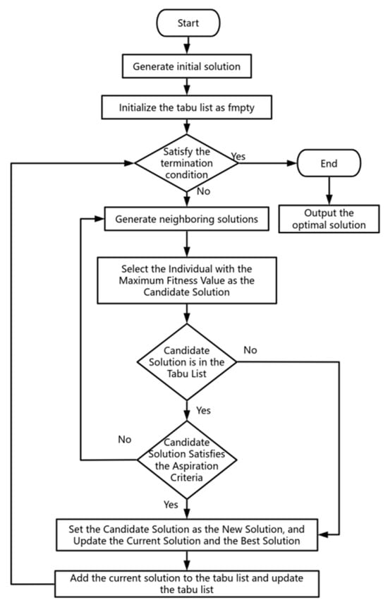
Figure 9.
Tabu search algorithm flowchart.
The flowchart of the multi-objective genetic local search algorithm is illustrated in Figure 10.
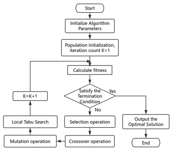
Figure 10.
Multi-objective genetic local search algorithm flowchart.
4. Improved Multi-Objective Genetic Algorithm
The multi-objective genetic local search algorithm demonstrates strong performance in escaping local optima. However, in non-convex search spaces, it becomes challenging to obtain solutions on the non-convex sections of the Pareto front. The selection of weights plays a crucial role in determining the relative importance of each objective, making it a key factor in the optimization process.
For the multi-objective optimization problem in this study, the two sub-objectives are conflicting—an improvement in one objective may lead to a decline in the performance of the other. This means that achieving an optimal solution for both objectives simultaneously is impossible. Instead, a trade-off and balance must be established between the two objectives to ensure that each objective function reaches its best possible state within the given constraints. The French economist V. Pareto (1848–1923) was among the first to study multi-objective optimization problems in economics and introduced the concept of the Pareto solution set [28]. Since multi-objective optimization problems inherently involve conflicting objectives, the optimal solution is not a single solution but rather a set of solutions. This set is known as the Pareto solution set, also referred to as the non-dominated solution set.
The Pareto optimal solution in a multi-objective optimization problem is merely an acceptable “non-inferior” solution, rather than a single absolute optimal solution. In most multi-objective problems, there are typically many Pareto optimal solutions. In practical applications, the selection of an optimal solution from the Pareto solution set depends on the understanding of the problem and the decision-maker’s preferences, where one or several solutions are chosen as the final optimal solution for the multi-objective optimization problem [29].
For a two-objective optimization problem, the non-dominated solution set forms a continuous or discrete curve in the objective space, which is referred to as the Pareto front.
Figure 11 shows the weighted sum diagram under dual objectives.
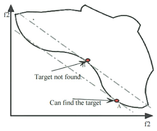
Figure 11.
Weighted sum diagram under dual objectives.
4.1. Adaptive Crossover and Mutation Probability
To address the above issues, this study first optimizes the crossover probability and mutation probability in the multi-objective genetic local search algorithm. Additionally, the fitness values of individuals in the population are incorporated as key reference indicators for determining both crossover and mutation probabilities, making the algorithm more adaptive to the actual state of the population. This improvement enhances the selection of high-quality individuals and facilitates a more efficient search for the global optimal solution [30].
- Adaptive Crossover Probability
Crossover operation is the core component of the genetic algorithm, facilitating gene recombination among individuals. Through crossover, the algorithm continuously generates new high-quality individuals, expands the search space, and ensures superior search performance. Since crossover probability serves as the sole indicator of crossover intensity, its selection is critically important. To enhance the adaptability of the algorithm, this study introduces an adaptive crossover probability, where the crossover rate is dynamically adjusted based on the fitness values of individuals in the population [31]. Instead of assigning zero or full crossover probability to the individuals with the highest and lowest fitness values, a specific probability is applied to ensure that the crossover operation effectively maintains population diversity within the algorithm.
The adjusted crossover probability is defined as:
where represents the fitness value of a specific individual in the population, is the maximum fitness value in the population, and is the minimum fitness value in the population.
- 2.
- Adaptive Mutation Probability
Mutation is an essential component of genetic algorithms. By applying a certain mutation probability to newly generated individuals, the algorithm ensures genetic diversity within the population. Mutation is typically combined with crossover operations to enhance the global search performance of the algorithm. When the algorithm approaches the optimal solution, an appropriate mutation operation can effectively accelerate convergence. The intensity of mutation is determined by the mutation probability , which has a significant impact on the overall performance of the algorithm. The mutation probability is usually small to prevent the loss of high-quality genetic material in the population. However, if the mutation probability is too high, the algorithm may shift towards random search, losing its structured optimization capability. Research indicates that in unimodal functions, the mutation probability is generally selected based on the dimension of the encoded string, and as the number of iterations increases, the mutation probability gradually decreases, improving convergence efficiency. In multimodal functions, an adaptive mutation probability is more suitable for real-world problems, offering greater adaptability [32].
The adjusted mutation probability is defined as:
where: represents the fitness value of a specific individual in the population, is the maximum fitness value in the population, and is the minimum fitness value in the population.
4.2. Improved Multi-Objective Genetic Local Search Algorithm I
Building on the optimization improvements in Section 4.1, it is important to recognize that the multi-objective fitness function evaluates each individual not only by considering the degree of constraint violations related to frequency assignment interference and the effectiveness of frequency reuse, but also by attempting to maximize the fitness value to guide the algorithm toward the optimal solution. By using the fitness function to evaluate individuals, the algorithm can effectively distinguish high-quality solutions from suboptimal ones, thereby facilitating convergence toward the overall optimization objective within the solution space.
For practical scenarios involving discrete composite objective functions, their integrals do not exist [33]. To prevent imbalance in the weight distribution of discrete objective functions, which could result in the failure to optimize certain objectives, it is necessary to perform random sampling within a pre-estimated non-dominated solution region. The discrete function values obtained through sampling are then used to determine the weight distribution of the composite objective function in a more reasonable and balanced manner [34].
For a set of discrete objective functions we can pre-estimate the function interval where non-dominated solutions are located or use an interval that fully encompasses all possible values of . By performing random sampling within this interval, a set of sampled function values can be obtained . For estimation convenience, the x-values selected for each function may vary. However, as long as the same number of sample values is randomly chosen for each discrete function, a rough estimation can be effectively performed.
Let:
First, each objective function should have a significant proportion in the composite objective function at the initial stage of the search, ensuring that the weight coefficients are assigned uniformly. This allows for a more balanced initialization, facilitating subsequent adjustments and trade-offs between different objectives [35]. By referring to the design principles of composite objective functions for continuous functions, the composite objective function in this case can be formulated as:
This method is referred to as the Mean Adaptive Method.
Based on Equations (16) and (23), the fitness function becomes:
where is the average interference count in the population, is the average frequency reuse factor in the population, and allmeanies refers to the average of and .
4.3. Improved Multi-Objective Genetic Local Search Algorithm II
By comparing Equation (19), the objective function of the Multi-Objective Genetic Local Search Algorithm, with Equation (16), it can be observed that the weights in the original objective function of the Multi-Objective Genetic Local Search Algorithm and the weights in the improved objective function follow the equivalence relationship [36]:
Even without making direct modifications to the Multi-Objective Genetic Local Search Algorithm itself, this equivalence relationship can still serve as a reference for estimating and determining the magnitude and range of all objective weight coefficients within the algorithm [37]. That is, in the Multi-Objective Genetic Local Search Algorithm, let:
Furthermore, the initial appropriate values for the objective weight coefficients can be determined based on this estimation. This estimation method, as defined in Equation (26), is referred to as the Mean-Guided Weighting Method.
Based on Equations (16) and (26), this becomes:
Based on Equation (27), the value of can be calculated, and subsequently, the value of can be determined.
5. Results and Conclusions
This section focuses on the frequency assignment problem for civil aviation navigation stations, utilizing five different multi-objective genetic algorithms for computation: the traditional multi-objective genetic algorithm, the multi-objective genetic algorithm with randomly assigned weights, the multi-objective genetic local search algorithm, the improved multi-objective genetic local search algorithm I, and the improved multi-objective genetic local search algorithm II. The results are then compared and analyzed to evaluate the performance of each algorithm.
To verify the effectiveness of the proposed algorithms, simulation experiments for both the original and improved versions were conducted using MATLAB 2020 software on a computer equipped with an Intel Core i7-10700 CPU, 16 GB of RAM, and running the Windows 11 operating system. This study focuses on the establishment of six VOR stations in Southwest China and addresses the frequency assignment problem using different algorithmic approaches.
In the traditional multi-objective genetic algorithm, the weight parameters are set as , with a crossover probability of and a mutation probability of . For both the multi-objective genetic algorithm with randomly assigned weights and the multi-objective genetic local search algorithm, the crossover and mutation probabilities remain the same as those in the traditional multi-objective genetic algorithm. In the adaptive crossover and mutation probability model, the parameters are set as K1 = 0.8, K2 = K5 = 1, K3 = K6 = 0.01, and K4 = 0.09. All other parameters remain consistent across the five algorithms. Based on preliminary experiments and considering the moderate complexity of the problem addressed in this study, a population size of 30 was found to achieve a good balance between solution quality and computational efficiency. The genetic algorithm is set to terminate after 1000 iterations, at which point the results are recorded to evaluate the optimization performance and convergence characteristics of each algorithm.
The information for some of the navigation stations in the Southwest China region is shown in Table 2, Table 3 and Table 4.
Table 2.
Information about established ILS stations.
Table 3.
Information about established VOR stations.
Table 4.
Information about the proposed VOR station.
Figure 12 shows the distance information of some stations, among which the distance calculation adopts the WGS84 model [38].
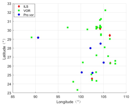
Figure 12.
Station distance information.
5.1. Weight Variation Analysis
The weight variation trends for the multi-objective genetic algorithm with randomly assigned weights, the multi-objective genetic local search algorithm, the improved multi-objective genetic local search algorithm I, and the improved multi-objective genetic local search algorithm II are shown in Figure 13, Figure 14, Figure 15 and Figure 16.
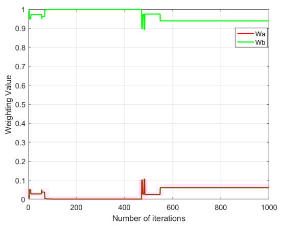
Figure 13.
Weight variation in the multi-objective genetic algorithm with randomly assigned weights.
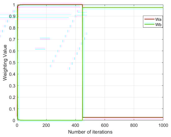
Figure 14.
Weight variation in the multi-objective genetic local search algorithm.
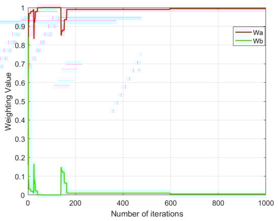
Figure 15.
Weight variation in the improved multi-objective genetic local search algorithm I.
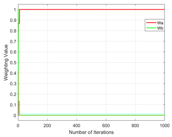
Figure 16.
Weight variation in the improved multi-objective genetic local search algorithm II.
From Figure 13, Figure 14, Figure 15 and Figure 16, it can be observed that different multi-objective genetic algorithms exhibit significant variations in weight convergence speed. The multi-objective genetic algorithm with randomly assigned weights shows the slowest convergence, with weights stabilizing only after approximately 550 iterations. The multi-objective genetic local search algorithm achieves stability slightly faster, converging around 460 iterations. In contrast, the improved multi-objective genetic local search algorithm I reaches weight stability much faster, at approximately 160 iterations, while the improved multi-objective genetic local search algorithm II demonstrates the fastest convergence, stabilizing in just 5 iterations.
By analyzing the relationship between weight variation trends and the number of iterations, it is evident that the multi-objective genetic algorithm with randomly assigned weights has the slowest weight stabilization speed among all tested algorithms. In contrast, the improved multi-objective genetic local search algorithm II achieves optimal convergence efficiency, requiring only a minimal number of iterations to stabilize the weights. This indicates that the improved multi-objective genetic local search algorithm II can adjust weight parameters more rapidly during optimization, thereby accelerating algorithm convergence and improving computational efficiency.
5.2. Fitness Value Comparison
The performance comparison of the five algorithms is shown in Figure 17.
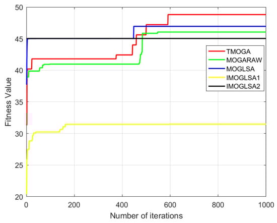
Figure 17.
Comparison of fitness values for five algorithms.
From Figure 17, it can be observed that different multi-objective genetic algorithms exhibit significant differences in convergence speed. Among them, the traditional multi-objective genetic algorithm has the slowest convergence speed, requiring a large number of iterations to reach a stable state during the optimization process. The multi-objective genetic algorithm with randomly assigned weights converges faster than the traditional method, indicating that the random weight assignment mechanism improves convergence efficiency, although it remains relatively slow. The multi-objective genetic local search algorithm achieves a slightly faster convergence rate than the randomly assigned weight algorithm, suggesting that the local search mechanism enhances convergence efficiency to some extent.
In contrast, the improved multi-objective genetic local search algorithm I and improved multi-objective genetic local search algorithm II demonstrate significantly faster convergence. In particular, the improved algorithm II, which incorporates the mean-guided weighting method, achieves the fastest convergence speed, reaching a stable state within very few iterations.
Overall, in terms of fitness convergence speed, the traditional multi-objective genetic algorithm is the slowest, while the improved multi-objective genetic local search algorithm II, benefiting from its enhanced optimization strategy, achieves the fastest convergence. This demonstrates that the mean-guided weighting method provides a substantial improvement in algorithm efficiency, allowing it to identify optimal solutions more rapidly and enhancing overall computational performance.
5.3. Optimization of Parameter A
In the design of the fitness function in this study, the selection of parameter A is critical to the performance of the algorithm, as it directly affects the quality of the final solution and the optimization effectiveness. Therefore, the following research will focus on the optimization of parameter A to improve the solution capability and overall performance of the algorithm.
When A = 0.01, the number of interference cases and the frequency reuse factor are shown in the figures below.
From Figure 18, it can be observed that when the parameter A = 0.01, the traditional multi-objective genetic algorithm achieves the highest frequency reuse factor, but its interference count reaches 3, indicating that the algorithm fails to effectively prevent interference during the optimization process. In contrast, all other algorithms achieve an interference count of 0, demonstrating their ability to effectively suppress interference while ensuring frequency reuse.
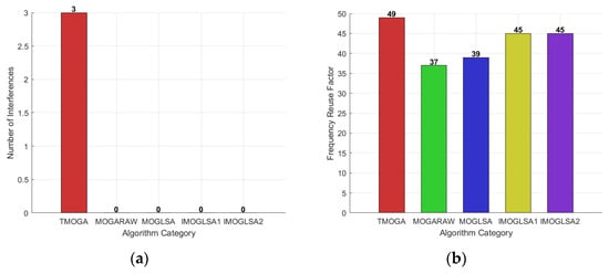
Figure 18.
(a) Illustrates the comparison of interference counts among five algorithms when A equals 0.01. (b) Illustrates the comparison of frequency reuse factors among five algorithms when A equals 0.01.
Among them, the improved multi-objective genetic local search algorithm I and improved multi-objective genetic local search algorithm II exhibit the best performance when A = 0.01, with both achieving a frequency reuse factor of 45, which is significantly superior to the other algorithms. This indicates that, under this parameter setting, these two improved algorithms not only maximize spectrum resource utilization but also obtain better solutions without interference.
When A = 0.02, the number of interference cases and the frequency reuse factor are shown in the figures below.
From Figure 19, it can be observed that when the parameter A = 0.02, although the traditional multi-objective genetic algorithm achieves the highest frequency reuse factor, its interference count also reaches the highest level, indicating that this algorithm poses a high interference risk during the optimization process, which negatively impacts the solution quality and stability.
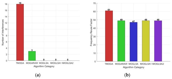
Figure 19.
(a) Illustrates the comparison of interference counts among five algorithms when A equals 0.02. (b) Illustrates the comparison of frequency reuse factors among five algorithms when A equals 0.02.
When A = 0.03, the number of interference cases and the frequency reuse factor are shown in the figures below.
From the Figure 18, Figure 19 and Figure 20, it can be observed that when A = 0.03, the frequency reuse factor of all algorithms has significantly improved compared to when A = 0.01 and A = 0.02. This indicates that a higher A value enhances frequency reuse capability to a certain extent. However, at the same time, the number of interference cases also increases significantly, making the interference problem more pronounced compared to A = 0.01 and A = 0.02. This suggests that while higher frequency reuse is achieved, it may lead to more severe frequency conflicts.
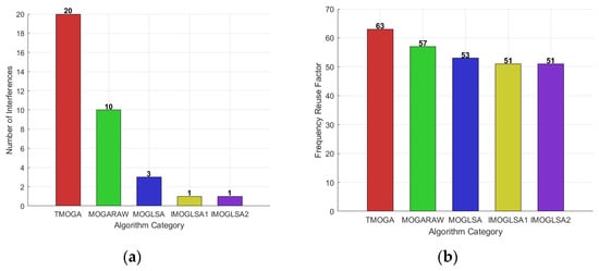
Figure 20.
(a) Illustrates the comparison of interference counts among five algorithms when A equals 0.03. (b) Illustrates the comparison of frequency reuse factors among five algorithms when A equals 0.03.
Overall, when A = 0.02, the five multi-objective genetic algorithms achieve their best overall performance. Under this setting, the algorithms attain a better balance between frequency reuse and interference control, demonstrating optimal optimization effects. Among them, the improved multi-objective genetic local search algorithm I and the improved multi-objective genetic local search algorithm II exhibit the lowest interference counts, indicating that these two optimized algorithms can effectively control interference while enhancing frequency reuse efficiency. This further validates the superiority of the improved algorithms in optimization performance, proving that they not only improve spectrum utilization efficiency but also better balance interference suppression and solution stability.
5.4. Comparison of Multi-Objective Optimization Algorithms
Finally, based on refs. [39,40], several commonly used multi-objective optimization algorithms (NSGA-II and MOEA/D) are compared with the two improved multi-objective genetic local search algorithms proposed in this study (IMOGLSA-I and IMOGLSA-II), as shown in Table 5.
Table 5.
Comparison of Multi-Objective Optimization Algorithms.
Where G is the number of generations, N is the population size, M is the number of objective functions, T is the number of neighbors for each individual, and K is the number of new individuals attempted in each generation of local search.
Based on the compara0tive analysis in Table 5, in terms of time complexity, NSGA-II and TMOGA exhibit the highest computational cost, followed by MOEA/D. The time complexity of IMOGLSA-I/II is slightly higher than that of MOEA/D due to the incorporation of local search procedures.
In terms of parameter dependency, IMOGLSA-I/II exhibit significantly lower sensitivity compared to other algorithms. NSGA-II and MOEA/D rely heavily on precise tuning of parameters such as crossover rates, mutation rates, or weight vector configurations. TMOGA, on the other hand, depends strongly on the proper formulation of fitness functions, which can be highly problem-specific and require substantial expert knowledge. In contrast, IMOGLSA-I/II incorporate adaptive mechanisms that dynamically adjust algorithmic behavior during the search process, thereby reducing reliance on manual parameter tuning and improving the algorithm’s robustness and applicability in practical engineering scenarios.
In addition, the diversity maintenance strategy of IMOGLSA-I/II benefits from a hybrid framework that balances global exploration and local refinement. This combined approach results in a better spread and convergence of solutions across the Pareto front, without the need for intricate design of distance metrics or weight vectors.
More importantly, IMOGLSA-I/II excel in terms of engineering applicability. The algorithms requires only targeted parameter tuning for the local search component, are insensitive to initial population and control parameters, and feature a clear structure that is easy to implement.
In summary, although the time complexity of IMOGLSA-I/II is slightly higher than that of MOEA/D, the proposed algorithms demonstrate significant advantages in reducing parameter sensitivity, simplifying algorithmic structure, and enhancing engineering applicability. In the context of this study, IMOGLSA-I/II are more practical and effective compared to other mainstream multi-objective optimization algorithms.
5.5. Conclusions
This study focuses on the frequency assignment problem for aviation navigation stations and proposes a series of multi-objective genetic algorithms to improve spectrum utilization efficiency while minimizing interference. A mathematical model based on objective function optimization was constructed and solved using the traditional multi-objective genetic algorithm, the multi-objective genetic algorithm with randomly assigned weights, the multi-objective genetic local search algorithm, and two improved versions of the multi-objective genetic local search algorithm.
Experimental results show that the traditional multi-objective genetic algorithm converges slowly and is prone to local optima. The introduction of randomly assigned weights and local search mechanisms enhances algorithm performance to some extent. However, the best optimization performance is achieved by the improved multi-objective genetic local search algorithms I and II. Among them, Algorithm II exhibits the fastest convergence, highest weight stabilization, and the best solution quality across different parameter settings.
In addition, parameter tuning experiments on the fitness function revealed that all algorithms performed best when parameter A = 0.02. Under this configuration, the improved algorithms—particularly Algorithm II—achieve optimal trade-offs between maximizing frequency reuse and minimizing interference, further enhancing the robustness and applicability of the solutions.
Further comparative analysis shows that mainstream multi-objective optimization algorithms such as NSGA-II and MOEA/D exhibit high sensitivity to parameter settings, including crossover rates, mutation rates, and weight vector configurations. Moreover, their structural complexity and implementation cost are relatively high. In contrast, the proposed IMOGLSA-I and IMOGLSA-II integrate adaptive mechanisms and local search strategies, which not only reduce reliance on manual parameter tuning but also enhance algorithmic stability and practical applicability, all while maintaining favorable time complexity.
In conclusion, the proposed improved algorithms—especially IMOGLSA-II—demonstrate significant advantages in addressing the frequency assignment problem for aviation navigation stations, offering more efficient and stable optimization solutions for aviation spectrum management. Additionally, this research provides a reliable methodological framework that can be extended to other static frequency assignment problems and broader classes of multi-objective optimization tasks.
Author Contributions
B.H.: Conceptualization, data curation, formal analysis, investigation, methodology, validation, writing—original draft, writing—review and editing. Y.X.: conceptualization, resources, supervision, writing—review and editing. K.G.: methodology, software, writing—review and editing. T.G.: methodology, software, writing—review and editing. Y.G.: software, writing—review and editing. M.L.: software, writing—review and editing. Q.Z.: resources, supervision, writing—review and editing. All authors have read and agreed to the published version of the manuscript.
Funding
Central University Basic Business Fund Project (ZHMH2022-007); Sichuan Provincial Key Research and Development Project (2022YFG0353).
Data Availability Statement
The data presented in this study are available on request from the corresponding author.
Conflicts of Interest
The authors declare no conflicts of interest.
References
- Lehtilä, S.; Alén, A.; Korpisaari, P.; Himmanen, H. Spectrum regulation and frequency allocation in the context of a smart city–using the regulatory approach in Finland as an example. Inf. Commun. Technol. Law 2023, 32, 418–432. [Google Scholar] [CrossRef]
- Fan, X. Intelligent Radio Spectrum Management and Dynamic Spectrum Allocation Algorithm. In Proceedings of the 2024 International Conference on Power, Electrical Engineering, Electronics and Control (PEEEC), Athens, Greece, 14–16 August 2024; IEEE: New York, NY, USA, 2024; pp. 836–841. [Google Scholar]
- Wang, X. Performance Analysis of Frequency Channel Allocation Algorithms for Multi-Cell UAV Communications in Cellular Networks. In Proceedings of the 2022 IEEE 5th International Conference on Information Systems and Computer Aided Education (ICISCAE), Dalian, China, 23–25 September 2022; IEEE: New York, NY, USA; pp. 722–726. [Google Scholar]
- Department of Transportaion Federal Aviation Administration. FAA Order 6050.32b Spectrum Management Regulations and Procedures Manual; International Civil Aviation Organization: Montreal, QC, Canada, 2008; pp. 1–132. [Google Scholar]
- Kamali, B. An overview of VHF civil radio network and the resolution of spectrum depletion. In Proceedings of the 2010 Integrated Communications, Navigation, and Surveillance Conference Proceedings, Herndon, VI, USA, 11–13 May 2010; IEEE: New York, NY, USA, 2010; pp. F4-1–F4-8. [Google Scholar]
- International Telecommunication Union. Handbook on National Spectrum Management; International Telecommunication Union: Hasan Sharif, United Arab Emirates, 2015; pp. 76–84. [Google Scholar]
- International Civil Aviation Organization. ICAO Handbook on Radio Frequency Spectrum Requirements for Civil Aviation; International Civil Aviation Organization: Montreal, QC, Canada, 2013; pp. 1–7. [Google Scholar]
- International Civil Aviation Organization. Aeroautical Tele-Communication Volume V; International Civil Aviation Organization: Montreal, QC, Canada, 2013; pp. 4–12. [Google Scholar]
- Fu, Z.; Zhou, R. A smarter algorithm-IFR3+ FFR in wireless network to optimize frequency allocation. J. Phys. Conf. Ser. 2021, 1903, 012034. [Google Scholar] [CrossRef]
- Song, K. Research on multiple mobile communication frequency allocation methods. In Proceedings of the International Conference on Signal Processing and Communication Technology (SPCT 2021), Tianjin, China, 24–26 December 2021; SPIE: St Bellingham, WA, USA, 2022; Volume 12178, pp. 235–244. [Google Scholar]
- National Research Council; Division on Engineering; Physical Sciences; Board on Physics; Committee on Radio Frequencies; Panel on Frequency Allocations, and Spectrum Protection for Scientific Uses. Handbook of Frequency Allocations and Spectrum Protection for Scientific Uses; National Academies Press: Cambridge, MA, USA, 2015. [Google Scholar]
- Chen, J.K.; De Veciana, G.; Rappaport, T.S. Improved measurement-based frequency allocation algorithms for wireless networks. In Proceedings of the IEEE GLOBECOM 2007-IEEE Global Telecommunications Conference, Washington, DC, USA, 26–30 November 2007; IEEE: New York, NY, USA, 2007; pp. 4790–4795. [Google Scholar]
- Feng, C.; Luo, Y.; Zhang, J.; Li, H. An OFDM-based frequency domain equalization algorithm for underwater acoustic communication with a high channel utilization rate. J. Mar. Sci. Eng. 2023, 11, 415. [Google Scholar] [CrossRef]
- Gunantara, N. A review of multi-objective optimization: Methods and its applications. Cogent Eng. 2018, 5, 1502242. [Google Scholar] [CrossRef]
- Chan, J.W.T.; Chin, F.Y.; Ye, D.; Zhang, Y.; Zhu, H. Frequency allocation problems for linear cellular networks. In Proceedings of the Algorithms and Computation: 17th International Symposium, ISAAC 2006, Kolkata, India, 18–20 December 2006; Proceedings 17. Springer: Berlin/Heidelberg, Germany, 2006; pp. 61–70. [Google Scholar]
- Pirozmand, P.; Hosseinabadi, A.A.R.; Farrokhzad, M.; Sadeghilalimi, M.; Mirkamali, S.; Slowik, A. Multi-objective hybrid genetic algorithm for task scheduling problem in cloud computing. Neural Comput. Appl. 2021, 33, 13075–13088. [Google Scholar] [CrossRef]
- Katoch, S.; Chauhan, S.S.; Kumar, V. A review on genetic algorithm: Past, present, and future. Multimed. Tools Appl. 2021, 80, 8091–8126. [Google Scholar] [CrossRef]
- Han, S.; Xiao, L. An improved adaptive genetic algorithm. In SHS Web of Conferences; EDP Sciences: Les Ulis, France, 2022; Volume 140, p. 01044. [Google Scholar]
- Ishibuchi, H.; Nojima, Y.; Doi, T. Comparison between single-objective and multi-objective genetic algorithms: Performance comparison and performance measures. In Proceedings of the 2006 IEEE International Conference on Evolutionary Computation, Vancouver, BC, Canada, 16–21 July 2006; IEEE: New York, NY, USA, 2006; pp. 1143–1150. [Google Scholar]
- Ombuki, B.; Ross, B.J.; Hanshar, F. Multi-objective genetic algorithms for vehicle routing problem with time windows. Appl. Intell. 2006, 24, 17–30. [Google Scholar] [CrossRef]
- Alhijawi, B.; Awajan, A. Genetic algorithms: Theory, genetic operators, solutions, and applications. Evol. Intell. 2024, 17, 1245–1256. [Google Scholar] [CrossRef]
- Selçuklu, S.B. Multi-objective genetic algorithms. In Handbook of Formal Optimization; Springer Nature: Singapore, 2024; pp. 1007–1044. [Google Scholar]
- Li, B.; Guo, T.; Mei, Y.; Li, Y.; Chen, J.; Zhang, Y.; Tang, K.; Du, W. A multi-objective memetic algorithm with adaptive local search for airspace complexity mitigation. Swarm Evol. Comput. 2023, 83, 101400. [Google Scholar] [CrossRef]
- Civera, M.; Pecorelli, M.L.; Ceravolo, R.; Surace, C.; Zanotti Fragonara, L. A multi-objective genetic algorithm strategy for robust optimal sensor placement. Comput.-Aided Civ. Infrastruct. Eng. 2021, 36, 1185–1202. [Google Scholar] [CrossRef]
- Wang, Z.; Pei, Y.; Li, J. A survey on search strategy of evolutionary multi-objective optimization algorithms. Appl. Sci. 2023, 13, 4643. [Google Scholar] [CrossRef]
- Xie, J.; Li, X.; Gao, L.; Gui, L. A hybrid genetic tabu search algorithm for distributed flexible job shop scheduling problems. J. Manuf. Syst. 2023, 71, 82–94. [Google Scholar] [CrossRef]
- Umam, M.S.; Mustafid, M.; Suryono, S. A hybrid genetic algorithm and tabu search for minimizing makespan in flow shop scheduling problem. J. King Saud Univ.-Comput. Inf. Sci. 2022, 34, 7459–7467. [Google Scholar] [CrossRef]
- Mottaki, N.A.; Motameni, H.; Mohamadi, H. An effective hybrid genetic algorithm and tabu search for maximizing network lifetime using coverage sets scheduling in wireless sensor networks. J. Supercomput. 2023, 79, 3277–3297. [Google Scholar] [CrossRef]
- Gagné, C.; Sioud, A.; Gravel, M.; Fournier, M. Multi-objective optimization. In Heuristics for Optimization and Learning; Springer Nature: Cham, Switherland, 2021; Volume 906, p. 183. [Google Scholar]
- Zhang, J.; Ding, L.; Long, S. State Feedback Control for Vehicle Electro-Hydraulic Braking Systems Based on Adaptive Genetic Algorithm Optimization. Int. J. Intell. Syst. 2024, 2024, 3616505. [Google Scholar] [CrossRef]
- Contreras, R.C.; Morandin Junior, O.; Viana, M.S. A new local search adaptive genetic algorithm for the pseudo-coloring problem. In Advances in Swarm Intelligence: 11th International Conference, ICSI 2020, Belgrade, Serbia, 14–20 July 2020, Proceedings 11; Springer International Publishing: Berlin/Heidelberg, Germany, 2020; pp. 349–361. [Google Scholar]
- Cui, H.; Qiu, J.; Cao, J.; Guo, M.; Chen, X.; Gorbachev, S. Route optimization in township logistics distribution considering customer satisfaction based on adaptive genetic algorithm. Math. Comput. Simul. 2023, 204, 28–42. [Google Scholar] [CrossRef]
- Caramia, M.; Dell’Olmo, P.; Caramia, M.; Dell’Olmo, P. Multi-Objective Optimization. In Multi-Objective Management in Freight Logistics: Increasing Capacity, Service Level, Sustainability, and Safety with Optimization Algorithms; Springer: London, UK, 2020; pp. 21–51. [Google Scholar]
- Pereira, J.L.J.; Oliver, G.A.; Francisco, M.B.; Cunha, S.S., Jr.; Gomes, G.F. A review of multi-objective optimization: Methods and algorithms in mechanical engineering problems. Arch. Comput. Methods Eng. 2022, 29, 2285–2308. [Google Scholar] [CrossRef]
- Hu, M.; Wu, T.; Weir, J.D. An adaptive particle swarm optimization with multiple adaptive methods. IEEE Trans. Evol. Comput. 2012, 17, 705–720. [Google Scholar] [CrossRef]
- Mengting, L.; Darong, H.; Ling, Z.; Ruyi, C.; Kuang, F.; Yu, J. An improved fault diagnosis method based on a genetic algorithm by selecting appropriate IMFs. IEEE Access 2019, 7, 60310–60321. [Google Scholar] [CrossRef]
- Zhou, W. Image Dehazing Enhancement Algorithm Based on Mean Guided Filtering. J. Inf. Process. Syst. 2023, 19, 417–426. [Google Scholar]
- Kelly, K.M.; Dennis, M.L. Transforming between WGS84 realizations. J. Surv. Eng. 2022, 148, 04021031. [Google Scholar] [CrossRef]
- Do, A.V.; Neumann, A.; Neumann, F.; Sutton, A. Rigorous runtime analysis of MOEA/D for solving multi-objective minimum weight base problems. Adv. Neural Inf. Process. Syst. 2023, 36, 36434–36448. [Google Scholar]
- Zheng, W.; Doerr, B. Runtime analysis for the NSGA-II: Proving, quantifying, and explaining the inefficiency for many objectives. IEEE Trans. Evol. Comput. 2023, 28, 1442–1454. [Google Scholar] [CrossRef]
Disclaimer/Publisher’s Note: The statements, opinions and data contained in all publications are solely those of the individual author(s) and contributor(s) and not of MDPI and/or the editor(s). MDPI and/or the editor(s) disclaim responsibility for any injury to people or property resulting from any ideas, methods, instructions or products referred to in the content. |
© 2025 by the authors. Licensee MDPI, Basel, Switzerland. This article is an open access article distributed under the terms and conditions of the Creative Commons Attribution (CC BY) license (https://creativecommons.org/licenses/by/4.0/).