Abstract
The wind tunnel experiment process is a nonlinear process with complex process characteristics. It is the primary task to master the key physical parameters and performance evaluation criteria during its operation. Aiming at the characteristics of multi-mode, multi-stage and intra-stage changes in the wind tunnel process, this paper proposes a Mach number prediction method based on mode, stage and intra-stage division. Firstly, mode division is carried out. The K-means clustering method is mainly used to cluster process data. The elbow rule is used to determine the cluster number K. The Mach number is used as the index variable to divide the process into phases, and divide the phases into stable parts and transitional parts according to different process characteristics. Considering the nonlinearity of the data, a kernel partial least squares prediction model is constructed for the stable process. Considering the dynamic characteristics of data, a dynamic partial least squares prediction model is constructed for the transitional process. The proposed method has been applied to multi-stage nonlinear wind tunnel experiments, and satisfactory results have been obtained.
1. Introduction
In recent years, aviation and aerospace technology has made great progress. China independently developed and designed the first domestic large aircraft C919. The Chang e-6 probe successfully landed in the South Pole Aitken basin on the far side of the moon, etc. The development, design and application of these aircraft cannot be separated from the progress of aerodynamic experiments and aerodynamic theory research. In this context, wind tunnel experimental facilities are crucial to the development of aviation and spacecraft, and they play a crucial role in the design phase. With the continuous progress of wind tunnel technology, its application scope has far exceeded the traditional aviation field, and now in bridge engineering, high-rise building design, and even the development of automobiles and railway vehicles, wind tunnels have played an important role. Wind tunnel experiments are mostly nonlinear processes with complex process characteristics. It is the primary task to master the key physical parameters and performance evaluation criteria during their operation. Among these, Mach number, as the core index used to measure the performance of a wind tunnel, is very important for accurate measurement. However, the Mach number cannot be directly obtained by means of measurement, especially in the multi-stage operation of the wind tunnel system, which requires indirect measurement methods to determine the Mach number. Therefore, variable analysis and prediction methods based on data analysis and mining methods have attracted the attention of most researchers.
Regarding the wind tunnel experiment process, Zhang Tingfeng et al. [1] used various model recognition methods to identify the parameters of the wind tunnel flow field related to the nonlinear block structure model of the wind tunnel system. Du Ning et al. [2] adopted the neural network method to devise a Mach number prediction model of the wind tunnel process. Zhao Hongyan et al. proposed to use regression analysis to identify and filter outliers in the data [3], so as to improve the performance of the prediction model. The model identifies outliers based on model residuals. When the residuals of a certain data point exceed the threshold, this point will be judged as an outlier and then processed. Zhao et al. analyzed the different operating modal characteristics of the wind tunnel, and proposed the algorithm of Mach number prediction based on the nonlinear autoregressive exogenous model (NARX)–Elman network model and model migration based on the input–output slope/bias correction–genetic algorithm (IOSBC-GA) model [4].
In the process of Mach number control for a wind tunnel, it has been found that the Mach number control effect is affected by the process running stage. In traditional methods, a unified model is established for the wind tunnel process in one mode, without distinguishing between the stable state and the transitional state. When the wind tunnel process runs smoothly, the Mach number prediction model that is established is more accurate and the prediction effect is better, while the control precision based on the Mach number prediction effect is higher. However, when the wind tunnel process is undergoing transition from one stable state to another, the established Mach number prediction model often cannot accurately capture the process characteristics, and the prediction effect is poor. This shows that to further improve the control accuracy of the Mach number, it is necessary to further divide the wind tunnel process into modes and stages, as well as intra-stage stable and transitional parts. Therefore, the changes in wind tunnel process characteristics are the focus of this work.
Changes in general process characteristics can be described as multi-modal and multi-stage. For complex production processes, multiple groups of similar and complete production processes form a mode, and different production settings give rise to different characteristics between modes. The stage generally refers to the different production states at work in a complete production process; that is, the completion of production must go through different production states. When the capturing of characteristics between stages alone is not enough to meet the needs of analysis, researchers have further proposed characteristic analysis within stages. Based on the analysis of the characteristics of complex industrial processes, multi-modal, multi-stage and intra-stage divisions were carried out, and on this basis, process monitoring and prediction models were established to improve batch process monitoring and quality prediction effects [5,6,7]. However, for the wind tunnel process, detailed analyses and studies of process characteristics are not enough, and further studies are needed. As introduced before, few works on wind tunnels deal with the multiplicity or unstable characteristics of the wind tunnel process. Researchers tend to adopt techniques focused on certain stable wind tunnel processes, which only represent a part of the wind tunnel process. Actually, during the wind tunnel test, multiple test settings arise due to different test requirements. Meanwhile, unstable transitions exist between stable states, and the control accuracy of the Mach number obviously decreases as the process of predicting the Mach number is not accurate enough.
As a typical method for the statistical analysis of multivariate data, partial least squares (PLS) has been widely used in statistical modeling, process monitoring, quality prediction and control [8,9,10]. At present, in the field of quality prediction, PLS plays a key role. The partial least squares method can filter the data and retain the independent variables that have a greater impact on the dependent variables, thus reducing the number of variables and making the model simpler and more efficient. In 1995, Nomikos P. and MacGregor J.F. [11] used statistical analysis technology to extract the principal components of input variables, take these principal components as predictive variables, and establish regression models with the final desired variables, thus improving process control and optimization. Wang En and Kowalski B.R. [12], MacGregor J.F. [13], and Wold S. [14] proposed multi-block partial least squares and hierarchical partial least squares. Rosipal and Trego [15] constructed a kernel partial least square model and added a kernel function, namely, KPLS, on the basis of PLS. By introducing a kernel function, the data are mapped to high-dimensional feature space, and the PLS algorithm is executed in this high-dimensional space, such that KPLS can capture the nonlinear relationships in the data. In terms of calculation, since there is no need to explicitly calculate the coordinates in the high-dimensional space, the calculation burden is reduced. At the same time, kernel technology effectively solves the problem caused by strong nonlinear industrial process data. This method is widely used to deal with nonlinear multivariable regression [16]. Dayal and Mac Gregor J.F. [17] adopted dynamic modeling techniques that can be used for online process monitoring, allowing models to be automatically updated over time so as to reflect process changes. The traditional PLS method achieves good performance when the input and output are static, but it shows limitations when dealing with dynamic changes. Therefore, methods such as dynamic structure are introduced into the PLS model to describe the dynamic characteristics of the system, a process known as dynamic PLS (DPLS) [18,19]. Despite these achievements, little research has been performed on the problem of characteristic variations caused by different operating conditions in wind tunnel processes. Due to its complex multi-modal, multi-stage, intra-stage and nonlinear characteristics, the accuracy and rapidity of the prediction methods of key variables need to be improved. It remains a challenge to analyze the multi-modal, multi-stage, intra-stage and nonlinear characteristics of wind tunnel processes.
In this paper, according to the characteristics of multi-mode, multi-stage and intra-stage changes in the wind tunnel process, a three-layer variable prediction method (multi-mode, multi-stage and intra-stage) is proposed. Firstly, the modal division of wind tunnel process data is carried out, and the K-means clustering method is mainly used to cluster process data. When determining the cluster number K of the K-means clustering method, the elbow rule is used to determine the cluster number. The stages are then identified by indicator variables. After the variable characteristic analysis of the wind tunnel process, the Mach number is used as the indicator variable, and thus the dynamic characteristic of the Mach number is analyzed, dividing the process into a series of stages. In addition, after dividing the stages, the process data are divided again within each stage, and the stage is further divided into the transitional part and the stable part within the stage. Considering the dynamic characteristics of data, a dynamic partial least squares prediction model is constructed for the transitional part. Considering the nonlinearity of the data, a kernel partial least squares prediction model is constructed for the stable part. Finally, the proposed method is applied to the wind tunnel experiment.
The rest of this paper includes the following sections: Section 2 focuses on the proposed methods, where the wind tunnel process is firstly introduced and then the model partitioning algorithm is developed based on K-means clustering. Further, the wind tunnel process is divided into multiple stages and intra-stage parts. Corresponding Mach number prediction methods are proposed for stable and transitional intra-stage parts. In Section 3, the method proposed in this paper is applied to the relevant wind tunnel. The results are then illustrated and compared with conventional methods. Finally, a summary of this paper is presented.
2. Methodology
This section mainly introduces the physics and control structure of wind tunnels, the modal division of tunnel processes, and stage division and modeling. Wind tunnel process data analysis is performed, after which we cluster using the K-means method, and then determine the number of clusters using the elbow rule to obtain final clustering results. Based on the characteristics of Mach numbers in multi-stage nonlinear wind tunnel processes, the stages are further divided, and within each stage, the data are divided into transitional and stable parts. Then, different methods are used to predict the Mach numbers of the two parts, respectively.
2.1. Wind Tunnel Process
The main components of wind tunnels include fan systems, control systems, measurement systems, etc., and the forms of different types of wind tunnels are also different.
The main structure of a wind tunnel consists of multiple components, including a test section, a stable section, and a diffuser section. The experimental section is the core area for measuring and observing the subjects. The function of the stable section is to enhance the straightness of the airflow. The expansion section aims to reduce energy loss. Overall, the design of the wind tunnel aims to precisely guide and control the test airflow. There are two main types of drive systems for wind tunnels: temporary and continuous. The temporary impulse drive system is equipped with energy storage devices to store energy. They are charged before the experiment and can quickly release energy to generate high-speed airflow during the experiment. The continuous drive system generates airflow through fans or compressors, which has the advantage of providing stable airflow and is suitable for long-term experiments and testing. The wind tunnel measurement control system needs to be designed and implemented considering specific experimental requirements to ensure that the system can provide accurate and reproducible experimental results. With the development of technology, wind tunnel measurement and control systems are becoming increasingly automated and intelligent, greatly improving the system’s intelligence and safety.
There are many methods and standards for classifying wind tunnels. If classified according to the Mach number of the wind tunnel test section, they can be divided into the following categories: Low-speed wind tunnels with Mach numbers less than 0.4 are suitable for studying basic aerodynamics, wing design, aircraft stability, etc., and which, due to their low airflow velocity, simple fans or propellers can be used as driving systems. Subsonic wind tunnels, with a test section Mach number generally between 0.4 and 0.8, are used to study the aerodynamic characteristics of aircraft near the speed of sound, such as transonic flow phenomena. Due to the higher Mach number, the drive system of the subsonic wind tunnel also requires higher power to generate the required airflow velocity. Transonic wind tunnels have a test section Mach number between 0.8 and 1.2, and cover the area near the speed of sound. Within this speed range, the properties of the airflow undergo significant changes, requiring special design in the wind tunnel to simulate these conditions. Therefore, transonic wind tunnels are also used to study the aerodynamic characteristics of aircraft during supersonic flight, such as the formation of shock waves and expansion waves. Supersonic wind tunnels, with a test section Mach number between 1.2 and 5.0, are used to simulate the aerodynamic characteristics of aircraft at extremely high speeds, such as shock wave interactions, high-temperature effects, etc. Their design and operation are more complex, requiring the use of high-pressure gas storage and rapid release systems to generate high-speed airflow. Hypersonic shock wave wind tunnels, which are specifically designed to generate shock waves and simulate hypersonic flow conditions, have a very high Mach number in the test section, even exceeding 20. Therefore, they usually use special compression techniques to generate brief hypersonic airflow.
This article focuses on the accurate prediction of Mach number in a 0.6 m continuous transonic wind tunnel.
This wind tunnel uses dry air as the experimental medium and is a closed loop wind tunnel with low noise and adjustable density. In addition, this wind tunnel provides important reference values for the research and construction of large wind tunnels, helping to reduce risks. The main components and structure of the 0.6 m continuous transonic wind tunnel are shown in Figure 1 [4].
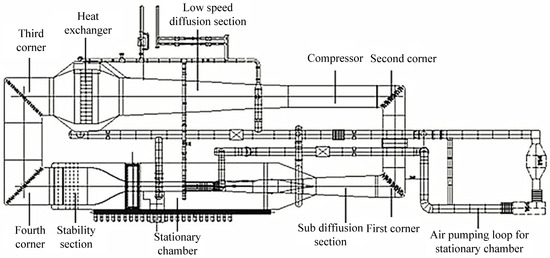
Figure 1.
Structural diagram of a continuous transonic wind tunnel.
Before each wind tunnel test, it is necessary to prepare the experimental model, and after the equipment is installed, the staff will inspect all devices. Then, the experimental parameter settings will be confirmed, ensuring that the parameters are correct, and the wind tunnel can be started. Wind tunnel valves and regulating devices are used to adjust parameters such as airflow velocity, temperature, and humidity to meet experimental requirements. Simultaneously, the airflow parameters are monitored to ensure their stability during the experimental process. The data collection system records the actual airflow parameters for the subsequent recording and analysis of experimental data that can be used to evaluate model performance. At the same time, the angle of attack continuously changes so as to achieve the goal of changing the Mach number.
2.2. Modal Partitioning Based on K-Means Clustering
Wind tunnel processes typically occur in different modes as production progresses, due to various production settings or environmental changes. Although similar production goals can be achieved in different production modes, when using the same model, one cannot accurately capture production characteristics. Therefore, for multiple modes, it is usually necessary to establish corresponding process models. Accurate modal partitioning plays a crucial role in the correct modeling of modalities. Here, K-means is used to perform the modal partitioning of the wind tunnel process.
The K-means algorithm is a commonly used partition clustering method. Given a dataset D of n data objects and the number of clusters to be generated K, the partitioning algorithm organizes the data objects into K (K ≤ n) partitions, where each partition represents a cluster.
Assuming dataset D contains n objects in Euclidean space, the partitioning method assigns objects in D to k clusters , , …, , such that for 1 ≤ i, j ≤ K, and =, minimizing the sum of squared errors E for all objects in the dataset.
Among them, Ci is the i-th cluster, o is the object in cluster Ci, ci is the centroid of cluster Ci, which is the average of all objects in the cluster.
In the formula, is the number of objects in cluster Ci.
The basic process of the K-means algorithm is as follows:
- Firstly, input the value of K—that is, the dataset with n objects will be clustered to obtain K classifications or groups;
- Randomly select K objects from dataset D as cluster centroids, with each cluster centroid representing a cluster. The resulting set of cluster centroids is ;
- For each object oi in D, calculate the distance between oi and ci (i = 1,2,…, K) to obtain a set of distance values. Select the cluster centroid Cs corresponding to the minimum distance value, and then divide the object oi into clusters with Cs as the centroid;
- Based on the set of objects contained in each cluster, recalculate the average value of all objects in the cluster to obtain a new cluster centroid, and return to step 3 until the cluster centroid no longer changes.
The entire process is shown in Figure 2.
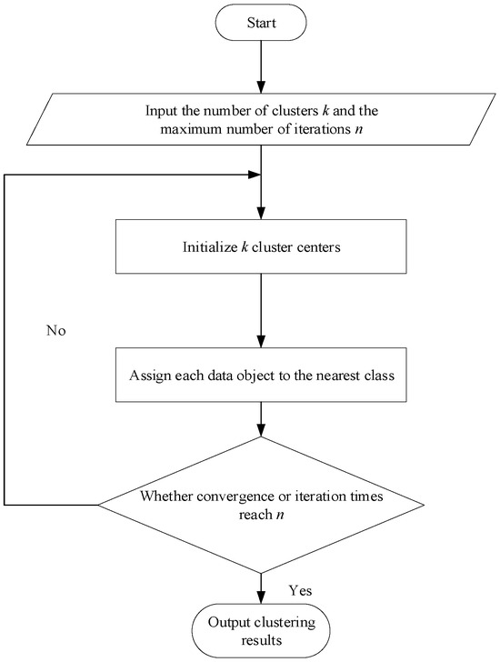
Figure 2.
K-means algorithm process.
The steps of the K-means algorithm are to preliminarily divide the data into K groups, randomly select K objects as initial cluster centers, then calculate the distance between each object and each seed cluster center, and assign each object to the nearest cluster center. The cluster centers and the objects assigned to them represent a cluster. For each sample assigned, the cluster centers will be recalculated based on the existing objects in the cluster, which repeats until a certain termination condition is met. The termination condition can be that no (or a minimum number of) objects are reassigned to different clusters, no (or a minimum number of) cluster centers change again, and the sum of squared errors is locally minimized.
The K-means algorithm is simple and efficient, making it a great clustering algorithm that is suitable for clustering large amounts of high-dimensional numerical data. When using the K-means clustering algorithm, the number of clusters k must be given first; that is, the data need to be clustered into k clusters. For this purpose, the elbow rule [20] is used to determine the value of k.
The elbow rule is achieved by establishing a cost function, as below:
Here, J is the cost function, x is an element in cluster Ci, and as the number of clusters increases, J will naturally become smaller. When K is less than the actual number of clusters, the increase in K will greatly increase the clustering degree of each cluster, so the decrease in J will be significant. When K reaches the true number of clusters, the regression of the clustering degree will rapidly decrease with the increase in K. In other words, the relationship diagram between J and K is the shape of an elbow, and the value of K corresponding to this elbow is the actual number of clusters in the data.
2.3. Multi-Stage Process Partitioning and Modeling
After analyzing the modal characteristics of the wind tunnel process, the next step is to divide the process within each mode into stages, as well as the stable and transitional parts within each stage. Due to changes in experimental requirements, the wind tunnel process generally has multiple stages, which means there are multiple stable parts within different stages required to meet production or experimental needs, as well as multiple transitional parts required to complete the transition between stages. Generally speaking, key variables in wind tunnel processes can reflect the stage characteristics of the process. It is feasible to use key variables as indicator variables for stages and internal changes within stages. Due to changes in the process operating variables, the key variables of the process exhibit stage changes over time. During each stable part, the process maintains a stable working state to meet its experimental needs. During the transitional part within each stage, the process transitions from one stage to the next, completing the change of the stage. It should be noted that in the wind tunnel process studied here, the key variables can be obtained through calculation or soft sensing methods at every moment, which means that the key variables can be continuously obtained. That is to say, each production mode and stage being stable or transitional does not affect the acquisition of key variables. This is fundamentally different from the intermittent production process consisting of multiple stages that ultimately obtain a quality variable.
Here, the process is divided into stages and internal-stage parts based on the key variable Mach number in the wind tunnel process. After partitioning, a mean KPLS model is established for Mach number prediction in each stable part, and a DPLS model is established for Mach number prediction in the transitional part.
2.3.1. Stage and Internal Division Based on Mach Number Data Features
Mach number () is the ratio of the speed of an object to the speed of sound, and plays the most important role in wind tunnel tests. Currently, there is no accurate device for measuring Mach number, and the data need to be calculated indirectly from the total and static pressure.
where P0 is the total pressure and Ps is the static pressure. This is the Mach number calculation formula when the adiabatic index of the air is 1.4 and the Ma is less than or equal to 1.
According to the analysis of the characteristics of Mach number data, it can be seen that the wind tunnel process exhibits significant stage changes due to changes in operating conditions. Meanwhile, there is a transitional section between the two stable processes. Normally, the collected Mach number contains a significant amount of noise. Thus the signal should be filtered before further analysis. Here, median filtering is adopted; this is a non-linear smoothing technique based on sorting statistics theory that can effectively suppress noise. The basic principle of median filtering is to replace the value of a point in a sequence with the median value of each point in its neighborhood, thereby eliminating isolated noise points. Afterwards, the differential value of Mach number is used as an indicator for dividing the stage and the stable and transitional parts within the stage.
where k is the index of sample points.
In this research work, the variation of Mach number is caused by control operation adjustment, and in order to simplify the process, the duration of each stage is fixed. Therefore, it is believed that the duration of the stable and transitional parts in each stage is consistent. After analyzing the Mach number changes in each stage separately, the average of the analysis results of the stable and transitional parts in each stage is taken as the length of the stable and transitional parts.
2.3.2. Stable Partial Mach Number Prediction Based on KPLS
The measured multi-stage nonlinear wind tunnel process variable data are formed into a three-dimensional matrix, , according to the direction of the batch, the variable, and the time. I represents the number of batches, Jx represents the number of process variables, and K represents the number of samples within each batch. The K time slice matrices are decomposed along the time axis. is the real Mach number.
The data gap between the variables is large, and the experimental data used in this topic are all from the data collected in the real wind tunnel process, which lack a unified standard definition, so there is a large degree of inconsistency meaning the data cannot be used directly. At the same time, the difference in magnitude of each variable is also huge. If the data are directly applied, then it will weaken the magnitude of small variables, leading to the phenomenon of big data “covering up” small data, and making it difficult to establish an accurate prediction model. Therefore, pre-processing should be undertaken before applying the data to modeling.
For a set of sequence , the data after the normalization of each point are
where represents the largest value in the data series and represents the smallest value in the data series . In general, in order to finally compare the actual operation data, the output result of the model needs to be reverse-normalized, and the data after the reverse-normalization are
After normalization, and are obtained. The correlation between the process variable and the measured variable can be abstracted from X and Y. X is decomposed along the time axis to derive k time slice matrices, namely, Xk.
When applying PLS to Xk and Y, the time-slice PLS model is implemented.
We can abbreviate the above model to the regression form as follows:
Here, Tk and Uk are fractional matrices, Pk and Qk are load matrices, Ek and Fk are residual matrices, is the regression parameter matrix, and K is the total number of time slices. When considering a single dependent variable Y, the regression model is
where is the regression parameter.
Under certain working conditions, in order to avoid the influence of noise, the mean model can be obtained by averaging the regression parameters of the time slice model.
Here, is the average regression parameter for all regression coefficients.
In order to solve the nonlinear problem in a wind tunnel system, KPLS based on the kernel function is introduced. The process data are first projected in a nonlinear way into a partitioned region of high-dimensional space, and then studied in this high-dimensional space, which makes it easier to work with nonlinear data compared to when using low-dimensional space. KPLS can use the kernel function to calculate the regression coefficient in high-dimensional space [21].
In KPLS, we can select the kernel function as
where is an n-dimensional Euclidean space.
We can also calculate the inner product as
where kn is the kernel function, and x and z represent two vectors in the initial space. In general, kernel functions are different, and so are forms of computation. The expression of the Gaussian kernel function is
In this work, and are obtained by projecting the normalized process variable and dependent variable matrix X and y into a selected kernel space, and the regression coefficient is obtained by applying PLS modeling to the projected data.
Thus, the mean model can be obtained as
where is the average regression parameter.
2.3.3. Transitional Part Mach Number Prediction Based on DPLS
In this section, the Mach number for the transitional part is extracted, and considering the dynamic characteristics of the data, the DPLS prediction model for the transitional part is constructed.
It can be clearly seen from the principles and algorithms of PLS that PLS only extracts static relationships between inputs and outputs. In order to construct a dynamic PLS model, time lag input is used to extend the input matrix. That is, for each input variable, past time point data are added as an additional column to the input matrix. If the input matrix is originally shaped like [N, p], where N is the number of samples and p is the number of input variables, then after introducing time lag, the shape of the input matrix will change to [N, p × (L + 1)], where L is the order of time lag. Thus, firstly, the size of the time lag should be determined. In time series analysis, if there is autocorrelation in the sequence, that is, there is a certain correlation between the current value and the past value, then this correlation can be observed through the autocorrelation function (ACF).
The autocorrelation function calculates the correlation coefficient between a time series and itself at different time delays, and is used to measure the correlation between the values of the same time series at different time points. For the time series , the covariance formula of and is
The autocorrelation function of and is
The autocorrelation function is only related to the time interval. It is unrelated.
Thus, for a given , the definition of ACF is
However, ACF has certain drawbacks as it sometimes cannot reflect the true impact of each lag value in the sequence, and it contains interference from other intermediate lag terms. Therefore, the partial autocorrelation function (PACF) is adopted, which can help identify the independent effects of each specific lagged term in the sequence.
Conditional correlation is called partial autocorrelation. The calculation method is as follows:
The partial autocorrelation function for a given sample is
Among these, is the autocorrelation function of a stationary process.
In this article, PACF is used to determine the optimal order of the time lag. If the value of PACF suddenly drops to 0 after a specific lag point, then that lag point is the optimal order.
3. Illustration and Discussion
3.1. Experimental Conditions and Settings
A typical continuous transonic wind tunnel is considered in this work. The test section size reaches 0.6 m × 0.6 m × 2.7 m (height × width × length); the wind tunnel temperature range is 233~333 K; the design total pressure range is 0.02~0.4 MPa; the test section Mach number range is 0.3~1.5; the rated power of the main compressor can reach 5000 kW; the rated power of the auxiliary compressor reaches 1500 kW; the process data were collected in the stability section of the wind tunnel [4]. In the wind tunnel test, the angle of attack is changed according to the set speed and change range, which leads to a huge disturbance in the flow field. The Mach number can only be kept stable by adjusting the compressor speed.
In this paper, the real-time Mach numbers are between 0.750 and around 0.785 in the transonic velocity range, in which range the lead slit is set to 24 mm; the opening/closing ratio is set to 1.5%, the total pressure is set to 50 kPa at atmospheric pressure, and the angle of attack change speed is 0.1°/s.
3.2. Mode Division Results
In order to use the K-means clustering algorithm for modal partitioning, the number of clusters K must first be given; that is, the data must be clustered into several clusters. To achieve this, the elbow rule is adopted to determine the value of k. Through calculation, the relationship between J and k is obtained, as well as the relationship between ΔJ and k, as shown in Figure 3.
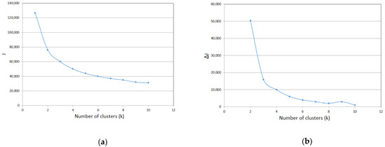
Figure 3.
(a) J and k relationship diagram; (b) ΔJ and k relationship diagram.
The elbow rule requires that the k value on the line segment ending at “elbow” be chosen as the best number of clusters. Here, the optimal value of k is the value of k before the curve starts to flatten out, that is, around k = 3, which can be seen from Figure 3a. After that, although k continues to increase, the decline in J is no longer so steep. This also can be concluded from Figure 3b. Therefore, the number of clusters selected for clustering is 3.
The K-means method is used to cluster all the data and divide them into three clusters. The clustering results are shown in Figure 4.
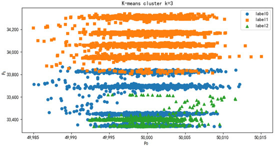
Figure 4.
K-means clustering results.
K-means clustering was used to successfully divide all data into three clusters. At the same time, in the original data set, each data point is marked with a category. Because the data set is relatively large, only the clustering result graph is shown here.
Figure 5 below is the Mach number timing diagram. The characteristics of the Mach number can be clearly seen from Figure 5. Firstly, it is divided into nine stages, and each stage is divided into a transitional part and a stable part. Regarding the purpose of achieving an accurate prediction of Mach number, it is obvious that it is more reasonable to gather the data of one stage into a cluster. However, it is obviously impossible to cluster every data point. For the previous clustering results, visualized with the Mach number, it is clear that the data from the fifth stage are clustered into two clusters. In order to ensure that the data of the same stage are gathered together, stage clustering is adopted.
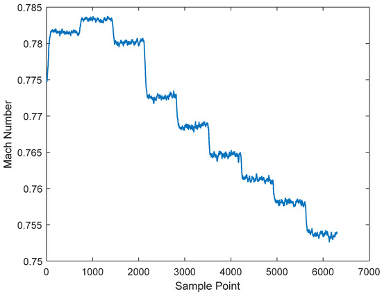
Figure 5.
Mach number timing diagram.
The stage clustering results are shown in Figure 6. A feature vector for each stage is created by calculating statistics such as the mean value and standard deviation of the data for each stage. These feature vectors are then used to run the K-means clustering algorithm to cluster the nine stages into three classes. Each point in Figure 6 represents a stage, and the color of the point indicates the cluster to which it belongs. Since there are nine stages, the scatter plot is drawn using two dimensions in the feature vector. Principal component analysis (PCA) is used to reduce the dimensionality of the eigenvector to find the two most important dimensions for plotting.
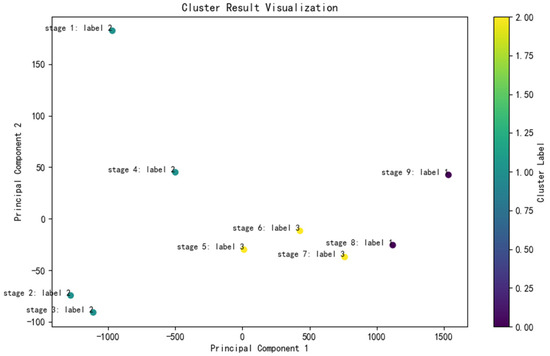
Figure 6.
Stage clustering results.
Through stage clustering, all stages have been successfully clustered into three categories, which is convenient for subsequent Mach number prediction. At the same time, the characteristics of the Mach number are further analyzed to divide each stage into the transitional part and the stable part. The results are shown in Figure 7; the filtered Mach number is shown in Figure 7a, and the difference in the Mach number is shown in Figure 7b. Finally, the first 46 data points of each stage belong to the transitional part, and the last 654 data points belong to the stable part. They are predicted separately in the following work.
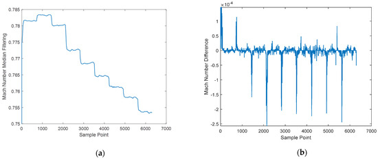
Figure 7.
Intra-stage division analysis, (a) median filtering results of Mach number, (b) Mach number difference.
3.3. Mach Number Prediction for Stable Parts
The Mach number of the stable part in a multi-stage nonlinear wind tunnel process is predicted by using the kernel partial least square method mentioned above. The predicted results are compared with those obtained by PLS.
First, the Mach number of cluster 1 is predicted. In cluster 1, the mean KPLS model is established, and the data in stages 1, 2 and 4 are respectively used to train the model and obtain the regression coefficient. Then, the trained model is used to predict the Mach number of the data block in stage 3, and the PLS prediction results are drawn in the graph for intuitive comparison. The predicted Mach number and the difference between the predicted Mach number and the actual Mach number are shown in Figure 8a,b.
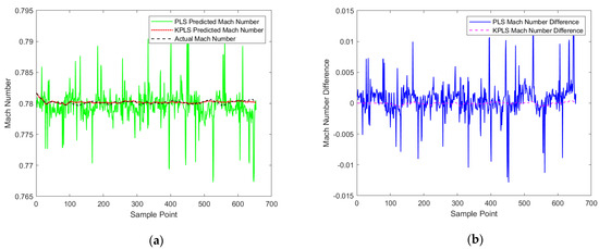
Figure 8.
Prediction results of Mach number under cluster 1, (a) Prediction curves, (b) Prediction difference curves.
Then, the Mach number of cluster 2 is predicted. In cluster 2, the mean KPLS model is established, and the data in stage 5 and 7 are used to train the model. Then, the trained model is used to predict the Mach number of the data block in stage 6, and a predicted value is obtained. The predicted Mach number and the difference between the predicted Mach number and the actual Mach number are shown in Figure 9a,b.
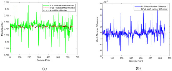
Figure 9.
Prediction results curves and difference curves of Mach number under cluster 2, (a) Prediction curves, (b) Prediction difference curves.
Then, the Mach number of cluster 3 is predicted. In cluster 3, the mean KPLS model is established, and the data in stage 8 are used to train the model. Then, the trained model is used to predict the Mach number of the data block in stage 9, and the predicted value is obtained. The predicted Mach number and the difference between the predicted Mach number and the actual Mach number are shown in Figure 10a,b.
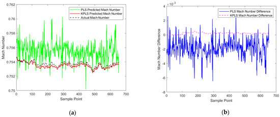
Figure 10.
Prediction results curves and difference curves of Mach number under cluster 3, (a) Prediction curves, (b) Prediction difference curves.
It can be seen from the above prediction results that no matter which cluster of Mach numbers is predicted, the prediction results of KPLS are much better than those of PLS. Then, the root-mean-square errors of the two are compared, as shown in Table 1. The results further prove that KPLS is better than PLS in predicting Mach number in the stable stage.

Table 1.
RMSE values of Mach number predictions for stable parts.
3.4. Mach Number Prediction for Transitional Parts
The optimal order of lag is determined using PACF, which shows the nonlinear correlation of the time series with its lag value. The results are shown in Figure 11.
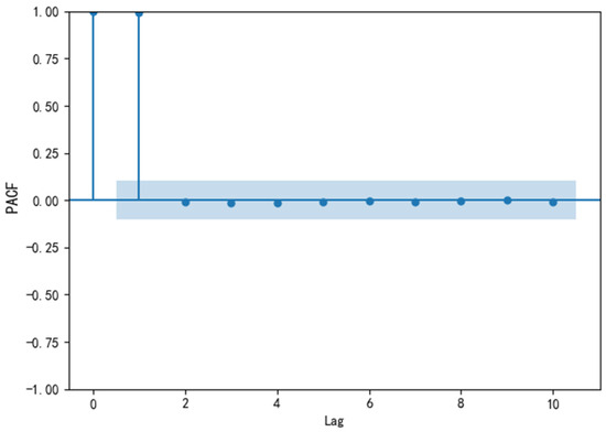
Figure 11.
PACF.
From a certain lag point, the PACF values all quickly drop below the 95% confidence interval. This cut-off point is generally considered to be the optimal lag point. From the PACF plot, it can be seen that after a lag of 2, the PACF value rapidly drops below the 95% confidence interval. Therefore, lag 2 can be selected as the best lag point.
In this paper, DPLS is used to predict the Mach number in the transitional stage, and the PLS prediction results are compared to observe whether the DPLS model is more suitable for predicting the Mach number in the transitional stage than the PLS model. Meanwhile, the difference between the predicted Mach number and the actual Mach number is calculated. The results obtained are shown in Figure 12a,b.
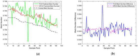
Figure 12.
Prediction results curves and difference curves of Mach number for transitional part, (a) Prediction curves, (b) Prediction difference curves.
By observation and comparison, we find that the predicted values of Mach number based on the traditional partial least square method and the dynamic partial least square method are both larger than the actual Mach number, but the predicted value of the latter is obviously more accurate than the former, and closer to the actual Mach number, so the effect is better in practice.
The root-mean-square error (RMSE) values of the two models were calculated to evaluate the prediction results.
The root-mean-square errors of both are shown in Table 2. Judging from the root-mean-square error of PLS and DPLS in predicting Mach number, we find that DPLS is also better than PLS in predicting Mach number.
Table 2.
RMSE values of Mach number predictions for the transitional part.
4. Conclusions
This article mainly focuses on Mach number prediction for wind tunnel processes to achieve the required prediction accuracy. Through a detailed analysis of the process characteristics, the wind tunnel process is divided into multiple modes, each of which is further divided into multiple stages, and each stage is further divided into internal stable and transitional parts. Mach number prediction models are established using KPLS and DPLS for the stable and transitional parts within different modes, respectively. Compared with traditional methods, the method proposed in this paper has higher prediction accuracy. In the future, research will be conducted at the data feature level to select features, using feature importance assessment methods to analyze the correlation between each feature and the Mach number, and remove features that are irrelevant or have a low correlation with the Mach number.
Author Contributions
Conceptualization, L.Z.; methodology, H.Y. and L.Z.; software, L.Z.; validation, J.G. and W.Y.; formal analysis, H.Y.; investigation, L.Z.; resources, J.G. and W.Y.; data creation, H.Y.; writing—original draft preparation, H.Y.; writing—review and editing, L.Z.; visualization, L.Z.; supervision, L.Z.; project administration, L.Z.; funding acquisition, L.Z. All authors have read and agreed to the published version of the manuscript.
Funding
This research was funded by the National Natural Science Foundation of China (No. 61503069) and the Fundamental Research Funds for the Central Universities (N2404010).
Data Availability Statement
All data used during the study were provided by a third party. Direct requests for data may be made to the provider, as indicated in the Acknowledgements.
Conflicts of Interest
Author Jin Guo was employed by the company Aviation Industry Corporation of China (AVIC). The remaining authors declare that the research was conducted in the absence of any commercial or financial relationships that could be construed as a potential conflict of interest.
References
- Zhang, T.; Mao, Z.; Yuan, P. A nonlinear block-oriented model for wind tunnel system. Inf. Technol. Control 2017, 46, 403–417. [Google Scholar] [CrossRef][Green Version]
- Du, N.; Long, X.; Zhao, L. A neural network based model predictive control for wind tunnel. In Proceedings of the 26th Chinese Control and Decision Conference (2014 CCDC), Changsha, China, 31 May–2 June 2014; pp. 2340–2343. [Google Scholar]
- Zhao, H.; Yu, D.; Wang, Y. Enhancing the prediction Mach number in wind tunnel with a regression-based outlier detection framework. Inst. Electr. Electron. Eng. 2021, 9, 27668–27677. [Google Scholar] [CrossRef]
- Zhao, L.; Shao, Y.; Jia, W. NARX-Elman based Mach number prediction and model migration of wind tunnel conditions. Aerospace 2023, 10, 498. [Google Scholar] [CrossRef]
- Hwang, D.; Han, C. Real-time monitoring for a process with multiple operating modes. Control Eng. Pract. 1999, 7, 891–902. [Google Scholar] [CrossRef]
- Lu, N.; Gao, F. Stage-based process analysis and quality prediction for batch processes. Ind. Eng. Chem. Res. 2006, 45, 2272–2280. [Google Scholar] [CrossRef]
- Zhao, L.; Zhao, C.; Gao, F. Inner-phase analysis based statistical modeling and online monitoring for uneven multiphase batch processes. Ind. Eng. Chem. Res. 2013, 52, 4586–4596. [Google Scholar] [CrossRef]
- Wold, S.; Ruhe, A.; Wold, H. The collinearity problem in linear regression: The Partial Least Squares (PLS) approach to generalized inverses. SIAM J. Sci. Stat. Comput. 1984, 5, 735–743. [Google Scholar] [CrossRef]
- Kourti, T.; MacGregor, J. Process analysis, monitoring and diagnosis, using multivariate projection methods. Chemom. Intell. Lab. Syst. 1995, 28, 3–21. [Google Scholar] [CrossRef]
- Gurden, S.; Westerhuis, J.; Bro, R.; Smilde, A. A comparison of multiway regression and scaling methods. Chemom. Intell. Lab. Syst. 2001, 59, 121–136. [Google Scholar] [CrossRef]
- Nomikos, P.; MacGregor, J. Multi-Way partial least squares in monitoring batch processes. Chemom. Intell. Lab. Syst. 1995, 30, 97–108. [Google Scholar] [CrossRef]
- Wangen, L.; Kowalski, B. A multiblock partial least squares algorithm for investigating complex chemical systems. J. Chemom. 1988, 3, 3–20. [Google Scholar] [CrossRef]
- MacGregor, J.; Jackle, C.; Kiparissides, C. Process monitoring and diagnosis by multiblock PLS methods. AIChE 1994, 40, 826–838. [Google Scholar] [CrossRef]
- Wold, S.; Kettaneh, N.; Tjessem, K. Hierarchical multiblock PLS and PC models for easier interpretation and as an alternative to variable selection. J Chemom. 1996, 10, 463–482. [Google Scholar] [CrossRef]
- Rosipal, R.; Trejo, L. Kernel partial least squares regression in reproducing kernel Hilbert space. J. Mach. Learn. Res. 2002, 2, 97–123. [Google Scholar]
- Zhang, X.; Kano, M.; Li, Y. Locally weighted kernel partial least squares regression based on sparse nonlinear features for virtual sensing of nonlinear time-varying processes. Comput. Chem. Eng. 2017, 104, 164–171. [Google Scholar] [CrossRef]
- Dayal, B.; MacGregor, J. Recursive exponentially weighted PLS and its application to adaptive control and prediction. J. Process Control 1997, 7, 169–179. [Google Scholar] [CrossRef]
- Kaspar, M.; Ray, W. Dynamic PLS modelling for process control. Chem. Eng. Sci. 1993, 48, 3447–3461. [Google Scholar] [CrossRef]
- Chen, J.; Cheng, Y.; Yea, Y. Multiloop PID controller design using partial least squares decoupling structure. Korean J. Chem. Eng. 2005, 22, 173–183. [Google Scholar] [CrossRef]
- Wu, G.; Zhang, J.; Yuan, D. Automatically obtaining K value based on K-means elbow method. Comput. Eng. Softw. 2019, 40, 167–170. [Google Scholar]
- Jia, R.; Mao, Z.; Wang, F. KPLS model based product quality control for batch processes. CIESC J. 2013, 64, 1332–1339. [Google Scholar]
Disclaimer/Publisher’s Note: The statements, opinions and data contained in all publications are solely those of the individual author(s) and contributor(s) and not of MDPI and/or the editor(s). MDPI and/or the editor(s) disclaim responsibility for any injury to people or property resulting from any ideas, methods, instructions or products referred to in the content. |
© 2025 by the authors. Licensee MDPI, Basel, Switzerland. This article is an open access article distributed under the terms and conditions of the Creative Commons Attribution (CC BY) license (https://creativecommons.org/licenses/by/4.0/).