Temporal-Sequence Offline Reinforcement Learning for Transition Control of a Novel Tilt-Wing Unmanned Aerial Vehicle

Abstract

A newly designed tilt-wing unmanned aerial vehicle (Tilt-wing UAV) requires a unified control strategy across rotary-wing, fixed-wing, and transition modes, introducing significant challenges. Existing control strategies typically rely on accurate modeling or extensive parameter tuning, which limits their adaptability to dynamically changing flight configurations. Although online reinforcement learning algorithms offer adaptability, they depend on real-world exploration, posing considerable safety and cost risks for safety-critical UAV applications. To address this challenge, we propose Temporal Sequence Constrained Q-learning (TSCQ), an offline RL framework that integrates an encoder–decoder with recurrent networks to capture temporal dependencies. The policy is further constrained within an offline dataset collected via hardware-in-the-loop simulation using a variational autoencoder, and a sequence-level prediction mechanism is introduced to ensure temporal consistency across action trajectories, thereby mitigating extrapolation error while preserving data fidelity. Experimental results demonstrate that TSCQ significantly outperforms gain scheduling, Model Predictive Control (MPC), and Batch-Constrained Q-learning (BCQ), reducing the RMSE of pitch angle by up to 53.3% and vertical velocity RMSE by approximately 33%. These findings underscore the potential of data-driven, safety-aware offline RL paradigms to enable robust and generalizable control strategies for tilt-wing UAVs.

1. Introduction

Tilt-wing UAVs have rapidly gained global prominence due to their fusion of vertical take-off and landing capabilities (VTOL), similar to quadrotors, and efficient forward flight reminiscent of fixed-wing aircrafts [1,2]. This dual-mode operational flexibility not only extends the UAV’s operational range—for example, in surveillance, disaster relief, and logistics—but also reduces infrastructural requirements by obviating conventional runways [3,4]. In the midst of increasing demand for advanced aviation and sustainable mobility solutions, the tilt-wing design exemplifies how innovative aerodynamic concepts can address both performance and environmental concerns [5,6]. Consequently, establishing reliable and versatile control strategies for such tilt-wing UAVs has broad implications for academia, industry, and government initiatives seeking to optimize aerial operations in increasingly complex environments [7].

Despite the clear advantages, controlling a tilt-wing UAV through its hover-to-cruise transition constitutes a major technical hurdle [8]. During this transition, significant changes in aerodynamic forces and control authority occur, compounded by dynamic coupling between the rotors, wings, and the airframe [9]. Rapidly changing angles of attack, lift distribution, and thrust vectors further complicate the real-time control problem.

Various strategies have been explored to address such transitional complexities. The robust $H^{\infty }$ gain-scheduled strategy relies on multiple linearized models and extensive parameter tuning [10], while MPC encounters computational overhead and demands accurate real-time models [11]. The sliding mode control is prone to chattering, affecting the accuracy of the control and reducing the life of the actuators [12]. Adaptive schemes such as dynamic inversion accommodate moderate model uncertainties but can diverge under severe parameter variations [13]. Recently, RL-based solutions have attracted attention as data-driven alternatives that reduce reliance on explicit modeling. Online RL, exemplified by proximal policy optimization (PPO), can discover near-optimal policies in simulated robotic tasks [14]. Furthermore, the deep-deterministic policy gradient (DDPG) and trust region policy optimization (TRPO) can also be used for control, but their performance is not as effective as the PPO algorithm [15]. Since online reinforcement learning typically does not involve real-flight trial and error but instead relies on virtual environments for online interaction, it requires a highly accurate simulation environment. In addition, the exploration process can generate extremely dangerous actions that can affect training efficiency and policy stability.

Offline RL has emerged as a safer learning paradigm by learning policies solely from more realistic precollected datasets, avoiding hazardous real-world exploration [16]. Compared to online RL, which trains policies in virtual environments, offline RL leverages more realistic offline data, making the learned policies more transferable to real-world deployment [17]. However, it contends with the “extrapolation error”, in which policies deviate into poorly represented action spaces, leading to inaccurate value estimates [18,19]. Although constraining policy actions to those well represented in the offline dataset can mitigate this issue, the newly designed tilt-wing UAV control remains particularly complex. This complexity arises from the fact that, across nearly all wing tilt angles, the system is inherently unstable, difficult to model precisely, and lacks accurate aerodynamic characteristics. As a result, model-based control methods often suffer from poor robustness due to their reliance on uncertain modeling assumptions [20,21]. To address these challenges, we collect offline datasets using hardware-in-the-loop simulations (HIL) and propose a temporal modeling approach within an offline RL framework, referred to hereafter as Temporal Sequence Constrained Q-learning (TSCQ). TSCQ enables the agent to understand the control patterns of the newly designed tilt-wing UAV in this study and generate optimal actions across different states. Furthermore, by capturing long-term dependencies, TSCQ provides predictive insights into future states [22], allowing the controller to anticipate rapid changes in aerodynamic forces and environmental factors. This predictive capability improves the ability to suppress potential adverse states in advance and improves the overall robustness of the control.

Ablation studies confirm that each component contributes to performance gains, with TSCQ consistently outperforming baseline controllers. It demonstrates superior robustness to abrupt transitions and unmodeled disturbances. By emphasizing data plausibility and temporal prediction, TSCQ achieves a balanced trade-off between safety, performance, and efficiency, making it well-suited for tilt-wing UAV control under safety-critical and exploration-constrained scenarios.

In summary, this paper presents an offline reinforcement learning framework that systematically curates offline data, integrates constrained policy learning [23] with temporal modeling to address multi-phase transitions, and includes ablation and comparative evaluations. The proposed TSCQ method provides a data-driven, safety-oriented control solution for a newly designed tilt-wing UAV. Simulation results show that TSCQ substantially reduces pitch angle ($\theta$) and pitch rate (q) errors. Specifically, the RMSE of $\theta$ is reduced by 51.6% compared to gain scheduling, 41.4% compared to MPC, and 53.3% compared to BCQ. Furthermore, vertical velocity error is reduced by approximately 33%.

The main contributions of our work are as follows.

• Hardware-in-the-loop (HIL) simulations, based on a flight control board with custom-modified control logic, are employed for offline data acquisition using the newly designed tilt-wing UAV model;
• We propose an offline reinforcement learning control algorithm named TSCQ, which leverages data-driven control for tilt-wing transitions. By incorporating additional predictive capability, the algorithm ensures the distributional consistency of entire action sequences;
• The superiority of the proposed method is validated through multiple comparative experiments and ablation studies conducted in the simulation.

The remainder of this paper is organized as follows. Section 2 introduces the mathematical model of the tilt-wing UAV. Section 3 details the offline data collection, augmentation, expert refinement, and dataset construction. Section 4 presents the offline RL training procedure and TSCQ implementation. Section 5 reports the ablation and comparative experiments. Section 6 concludes the paper and outlines future work.

2. Mathematical Model

In this section, we present a mathematical description of the controlled object model used in this study. Figure 1 shows a simplified top-down view of the tilt-wing UAV under investigation, transitioning from rotary-wing mode to fixed-wing mode ((a), (b), (c)) and then from fixed-wing mode back to rotary-wing mode ((c), (d), (a)). The white sections in the figure represent the fixed-wing control surfaces. The rigid internal components of UAVs are depicted by dashed lines in the figure. These components, when moved by a pushrod along the direction of the solid arrows, cause the wings to rotate around the joint.

The tilt-wing UAV model is symmetric in all configurations (rotary-wing, transition, and fixed-wing), and since control of the pitch channel is especially critical during the transition process [24], we aim to evaluate the feasibility and advantages of the proposed approach more efficiently. Therefore, we describe a three-degree-of-freedom (3-DOF) [25] longitudinal model of the tilt-wing UAV, which is derived based on the Newton and Euler theorems.

2.1. Coordinate System

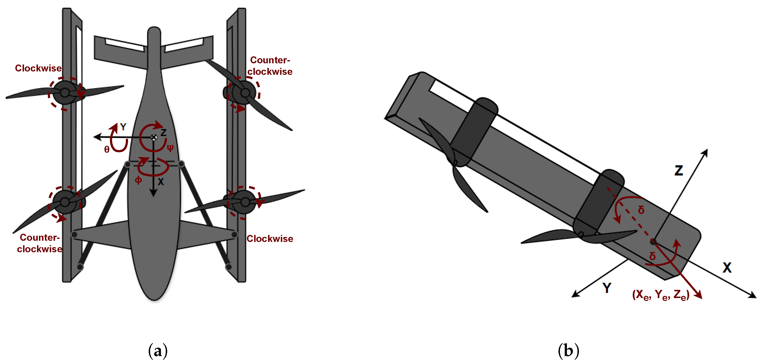
Three coordinate systems are primarily used: the ground coordinate system, the body-fixed coordinate system, and the wing-fixed coordinate system [26]. The ground coordinate system follows the conventional North–East–Down (NED) convention, with the origin located at the UAV’s center of gravity in rotary-wing mode. The body-fixed coordinate system follows the conventional Forward–Right–Down (FRD) convention (Figure 2a), with its origin located at the UAV’s center of gravity in rotary-wing mode. The figure also indicates that the front-right and rear-left rotors rotate counterclockwise, while the others rotate clockwise. This configuration cancels the net yaw torque, thereby supporting the symmetry assumptions in the torque model. The wing-fixed coordinate system is defined with the tilt-joint as the origin, with the x-axis pointing forward, parallel to the longer edge of the wing; the y-axis is directed to the right, perpendicular to the wing surface; and the z-axis is directed downward, parallel to the shorter edge of the wing (Figure 2b).

Before takeoff, the ground coordinate system and the body-fixed coordinate system coincide. After takeoff, the body-fixed coordinate system rotates relative to the geographic coordinate system. According to Euler’s theorem, the rotational motion of a rigid body about a point can be decomposed into several successive rotations around different axes. Therefore, the transformation between the geographic coordinate system and the body-fixed coordinate system can be achieved through three successive rotations about different axes [26]. The rotation angles of the body-fixed coordinate system around the three principal axes are known as Euler angles, which include the yaw angle $\psi$ (rotation about the Z axis), the pitch angle $\theta$ (rotation about the Y axis), and the roll angle $\varphi$ (rotation about the X axis). Their positive directions follow the right-hand rule. These rotations are illustrated using red curved arrows in Figure 2a.

This rotation can be represented as a sequence of three consecutive rigid-body rotations about different axes. In this study, we adopt a z–y–x rotation sequence for the coordinate transformation. Through straightforward mathematical derivation, the transformation matrix from the NED coordinate system to the body-fixed coordinate system is obtained as $R_e^b$, as shown in Equation (1).

$$R_e^b=\left(\begin{array}{ccc}cos\theta cos\psi & cos\theta sin\psi & -sin\theta \\ sin\theta cos\varphi cos\psi -cos\theta sin\varphi sin\psi & sin\theta cos\varphi sin\psi +cos\theta cos\varphi cos\psi & sin\varphi cos\theta \\ sin\theta sin\varphi cos\psi +cos\theta cos\varphi sin\psi & sin\theta sin\varphi sin\psi -cos\theta cos\varphi cos\psi & cos\varphi cos\theta \end{array}\right)$$

(1)

Since $R_e^b$ is an orthogonal matrix, the transformation matrix from the body-fixed coordinate system to the geographic coordinate system is given by $R_e^b={\left(R_b^e\right)}^{-1}={\left(R_b^e\right)}^T$. Using the rotation matrix for the transformation of the coordinate system, the conversion from the body-fixed coordinate system $(u,v,w$) and $(p,q,r$) to the three-axis velocity and angular rates of the ground coordinate system can be obtained. The details of this process are omitted here.

Now, we analyze the case where the wing rotates around the tilt-joint. Based on our analysis, this rotation can be described as a fixed-axis rotation in the wing-fixed coordinate system, with a rotation angle ranging from 0° to 120°, corresponding to the transition from rotary-wing mode to fixed-wing mode. During this rotation, the representation of the wing-fixed coordinate system in the body-fixed coordinate system can be expressed using the rotation matrix $R_w^b$, as shown in Equation (2).

$$R_w^b=\left(\begin{array}{ccc}{X}_e^2(1-cos\delta )+cos\delta & X_e{Y}_e(1-cos\delta )+Z_{e}sin\delta & X_e{Z}_e(1-cos\delta )-Y_{e}sin\delta \\ X_e{Y}_e(1-cos\delta )-Z_{e}sin\delta & Y_e^2(1-cos\delta )+cos\delta & Y_e{Z}_e(1-cos\delta )+X_{e}sin\delta \\ X_e{Z}_e(1-cos\delta )+Y_{e}sin\delta & Z_e{Y}_e(1-cos\delta )-X_{e}sin\delta & Z_e^2(1-cos\delta )+cos\delta \end{array}\right)$$

(2)

$X_e,Y_e,Z_e$ represent the unit vectors of the fixed axis for the tilt-wing mechanism, and $\delta$ denotes the tilt rotation angle. Taking the right wing as an example, its local tilt-axis orientation expressed in the body-fixed coordinate system is ${\widehat{e}}_r=\left({\displaystyle \frac{\sqrt{3}}{3}},-{\displaystyle \frac{\sqrt{3}}{3}},-{\displaystyle \frac{\sqrt{3}}{3}}\right)$. The positive direction of $\delta$ follows the right-hand rule about this axis. This convention is illustrated by red curved arrows in Figure 2b. The tilt-axis definition for the left wing is analogous by symmetry. Once we obtain the key matrix that describes the tilt transition process, we can characterize the forces and moments generated by the rotors in the pitch channel. The rotor thrust in both the wing-fixed coordinate system and the body-fixed coordinate system, as well as the rotor moments in the body-fixed coordinate system [27], can be expressed using Equation (3).

$$\left\{\begin{array}{c}{\overrightarrow{T}}_w={\displaystyle {\sum }_{i=1}^4}{\overrightarrow{T}}_i={\displaystyle {\sum }_{i=1}^4}\left[\begin{array}{c}0\\ 0\\ -k_t{\omega }_i^2\end{array}\right]\hfill \\ {\overrightarrow{T}}_b={\displaystyle {\sum }_{i=1}^4}{R}_w^b·{\overrightarrow{T}}_i\hfill \\ {\overrightarrow{M}}_b={\displaystyle {\sum }_{i=1}^4}(R_w^b·{\overrightarrow{T}}_i\times {\overrightarrow{L}}_i\left(\delta \right))\hfill \\ I_{yy}\left(\delta \right)=I_{yy}^{\mathrm{body}}+m\left[{\left(\Delta x_{\mathrm{cg}}\left(\delta \right)\right)}^2+{\left(\Delta z_{\mathrm{cg}}\left(\delta \right)\right)}^2\right]\hfill \end{array}\right.$$

(3)

${\overrightarrow{T}}_w$ represents the total thrust of the four rotors expressed in the wing-fixed coordinate system. Each rotor’s thrust vector is denoted as ${\overrightarrow{T}}_i$, where ${\overrightarrow{T}}_i$ is the thrust coefficient (with units $N{s}^2$), and ${\omega }_i^2$ is the rotational speed of the i-th rotor in radians per second. The transformation from wing-fixed to body-fixed coordinates is achieved through the rotation matrix $R_w^b$, yielding the total thrust vector ${\overrightarrow{T}}_b$ in the body-fixed frame. The total moment ${\overrightarrow{M}}_b$ in the body-fixed frame is calculated using the cross product of the transformed thrust $R_w^b·{\overrightarrow{T}}_i$ and the moment arm ${\overrightarrow{L}}_i\left(\delta \right)$, which denotes the vector from the tilt joint to the i-th rotor and is a function of the tilt angle $\delta$.

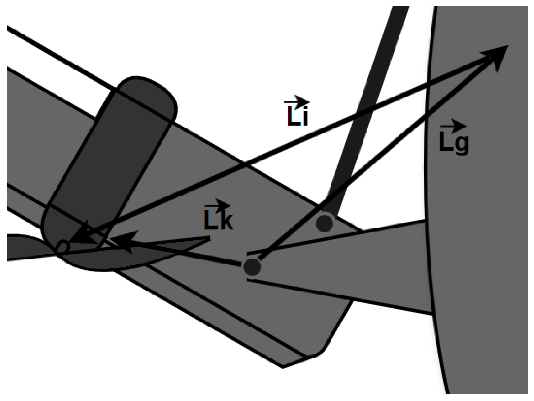
It is important to note that during the transition, the center of gravity shifts forward toward the nose. Therefore, we define the vector from the tilt-joint to the center of gravity as ${\overrightarrow{L}}_g\left(\delta \right)$ and the vector from the tilt-joint to the motor as ${\overrightarrow{L}}_k$. The moment arm can then be expressed as ${\overrightarrow{L}}_i\left(\delta \right)={\overrightarrow{L}}_k-{\overrightarrow{L}}_g\left(\delta \right)$ (Figure 3). As the center of gravity shifts during the transition, the pitch-axis moment of inertia also varies accordingly. Following the parallel axis theorem [28], we define the time-varying inertia $I_{yy}\left(\delta \right)$, where $I_{yy}^{\mathrm{body}}$ is the intrinsic moment of inertia of the UAV body about the pitch axis, and $\Delta x_{\mathrm{cg}}\left(\delta \right)$, $\Delta z_{\mathrm{cg}}\left(\delta \right)$ are the horizontal and vertical displacements of the center of gravity relative to the tilt joint, extracted from the defined vector ${\overrightarrow{L}}_g\left(\delta \right)$. This modeling approach captures the inertia variations caused by center-of-gravity shifts, thereby enhancing the physical fidelity of the dynamic model. All formulations follow the structure presented in Equation (3).

2.2. Model Description and Validation

In the previous subsection, we elaborated on the relationships between different coordinate systems, with a particular focus on the forces and moments generated by the rotors during the tilt transition. For the aerodynamic forces and moments of the fixed-wing mode, we conducted wind tunnel experiments to obtain experimental data under varying tilt progressions, angles of attack, and control inputs. Specifically, the number of configurations is five, corresponding to tilt progressions of $0, 0.25, 0.5, 0.75, 1$, which represent tilt angles $\delta =0^{\circ }, {30}^{\circ }, {60}^{\circ }, {90}^{\circ }, {120}^{\circ }$, respectively. These configurations cover the rotary-wing, transition, and fixed-wing modes.

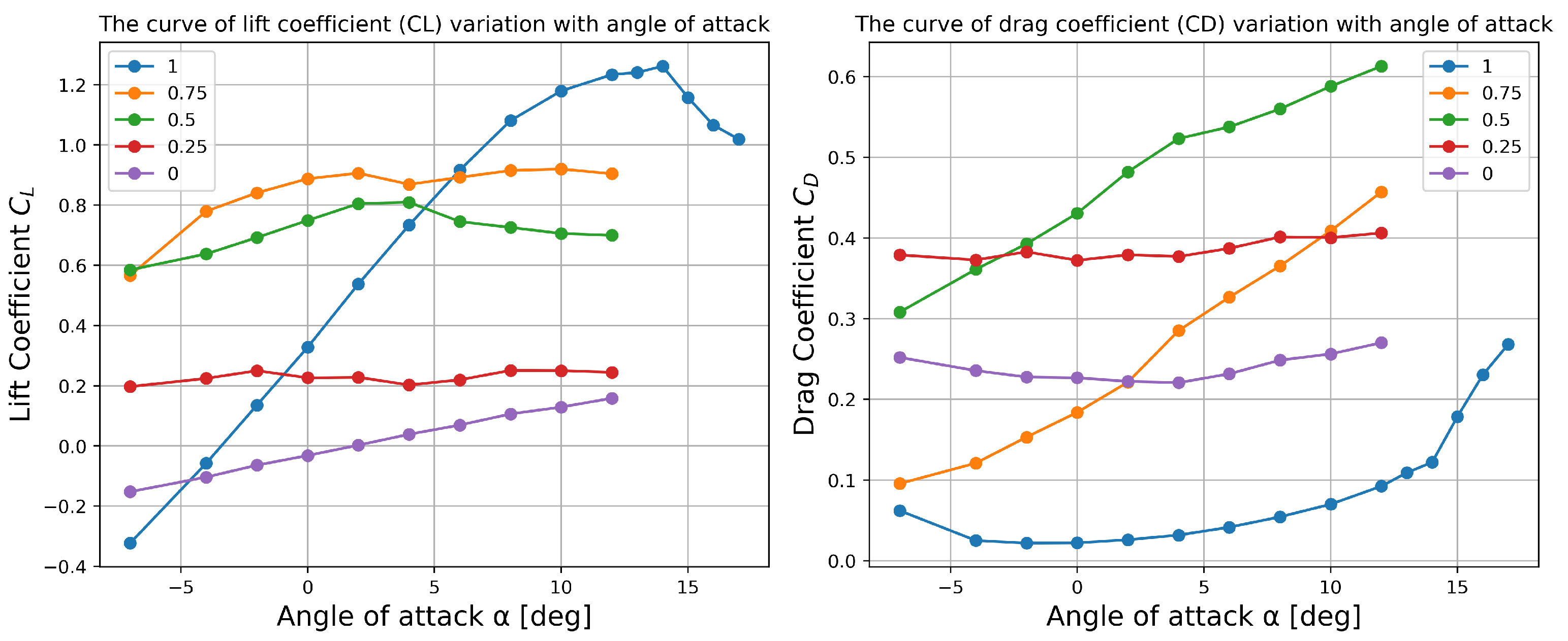
These data were processed using multidimensional interpolation [29] to ensure the validity of the data for any condition within a tilt progression range of 0–1, angle of attack range of −7° to +17°, and control input range of ±25°. Figure 4 presents the lift and drag coefficient curves under different tilt progressions and angles of attack. Analyzing the curves in the figure, when the tilt progression is 0, lift is provided primarily by the rotors, while the wings contribute almost no lift. When the tilt progression reaches 1, the lift variation with angle of attack exhibits characteristics typical of fixed-wing aerodynamics, where $C_L$ increases with the angle of attack initially, followed by a stall beyond a certain angle. Drag is mainly influenced by friction drag and pressure drag, with $C_D$ gradually increasing at first and then rising sharply after the stall angle [30]. At tilt progressions of 0.25, 0.5, and 0.75, $C_L$ gradually increases, indicating a growing contribution of aerodynamic lift from the fixed wings. $C_D$ becomes more sensitive to angle-of-attack variations, showing a transitional behavior on the curve.

Thus, the lift L and drag D can be written as in Equation (4), where $\rho$ is the air density (kg/m³), V is the relative airflow velocity (m/s), and S is the wing reference area (m²).

$$\left\{\begin{array}{c}L=0.5\rho V^{2}S{C}_L\left(\alpha \right)\hfill \\ D=0.5\rho V^{2}S{C}_D\left(\alpha \right)\hfill \end{array}\right.$$

(4)

Additionally, the coefficients of the forces and moments generated in the fixed-wing mode were measured through wind tunnel experiments, obtaining the increments in $C_L$ and $C_D$ per unit control surface deflection [31]. The specific details of the wind tunnel experiments are omitted here.

Finally, the longitudinal dynamics of the aircraft are derived as shown in Equation (5). The kinematic and dynamic formulations presented in this paper are applicable throughout the entire tilt process. By introducing the tilt angle $\delta$, the model maintains a structurally consistent form that unifies rotary-wing, transition, and fixed-wing modes under a single mathematical framework. Based on this unified model, we conducted extensive offline simulations to collect training data under various flight conditions and tilt configurations. The data generation process and coverage details are described in the following section.

$$\left\{\begin{array}{c}\dot{u}=-gsin\theta +(T_u-Dcos\alpha +Lsin\alpha +F_{cs})/m-qw\hfill \\ \dot{w}=gcos\theta +(T_w-Lcos\alpha -Dsin\alpha +F_{cs})/m+qu\hfill \\ \dot{x}=wsin\theta +ucos\theta \hfill \\ \dot{z}=wcos\theta -usin\theta \hfill \\ \dot{\theta }=q\hfill \\ \dot{q}=(m+M_{cs}+M_{wy})/I_{yy}\hfill \end{array}\right.$$

(5)

where g is gravity acceleration; $I_{yy}$ is the moment of inertia on the $Y_b$ axis, with its analytical formulation included in Equation (3); $\alpha$ represents the angle of attack; $\theta$ represents the pitch angle; m is the mass; and L and D denote lift and drag. $\dot{x}$ and $\dot{z}$ represent the horizontal and vertical velocities in the body-fixed coordinate system, respectively. q denotes the pitch angular velocity around the $Y_b$ axis. $F_{cs}$ and $M_{cs}$ represent the forces and moments generated by control inputs, while $M_{wy}$ accounts for the additional moment produced by the rotors. The terms $qw$ and $qu$ correspond to Coriolis force components.

$$\left\{\begin{array}{cc}\hfill T_u& =T·\left[X_e{Z}_e(1-cos\delta )-Y_{e}sin\delta \right]\hfill \\ \hfill T_w& =-T·\left[Z_e^2(1-cos\delta )+cos\delta \right]\hfill \end{array}\right.$$

(6)

Here, $T_u$ and $T_w$ are defined as shown in Equation (6), with their rotational relationship described by $R_w^b$. $M_{wy}$ represents the additional pitch moment generated by the rotors, as previously defined in Equation (3).

To evaluate both traditional control algorithms and offline reinforcement learning, it is essential to ensure that the experimental data and imported data are error-free. Therefore, we conducted 100 sets of interpolation and extrapolation validation tests using code under different conditions, including varying angles of attack, tilt progressions, and airspeeds. Furthermore, we verified the correctness of the rotation matrices of the coordinate system and performed single-step and iterative validation to confirm the precision of model construction [32]. Furthermore, by analyzing the printed results from the code, we examined the aerodynamic data, forces, and moments, manually confirming that all values fall within the correct range.

3. Offline Dataset Generation

Utilizing fixed offline datasets to record interactions for offline reinforcement learning is a critical consideration in real-world applications. Effective offline RL algorithms have a broader range of applications compared to online RL [33,34]. Since the agent learns solely from a previously collected static dataset, this paradigm enables policy extraction from large and diverse training datasets. However, it also imposes stringent requirements on the correctness and diversity of the offline dataset [35]. Insufficient diversity in the dataset can lead to overfitting, where the agent learns policies that are overly tailored to the specific distribution of the offline data. This overfitting results in poor generalization to previously unseen states during deployment. Moreover, it is essential that the reward structure within the dataset accurately reflects the environment’s feedback mechanism, ensuring that the learned policy is both effective and capable of outperforming strategies derived from the dataset itself. The agent’s ability to learn successful policies is directly influenced by the quality of the data, as any errors or biases present in the dataset can propagate throughout the learning process, compromising the overall performance. Consequently, enhancing the diversity and coverage of the offline dataset is crucial to the development of robust offline RL algorithms. This section will discuss various techniques employed in this study to create a diverse and comprehensive offline dataset, with a particular focus on capturing the full complexity of the environment while striking a balance between the dataset’s breadth and its relevance to the task.

3.1. Hardware-in-the-Loop Simulation Methodologies

The raw data for this experiment come from hardware-in-the-loop (HIL) simulations. In aircraft development, system simulation is essential and often the only feasible support method [36]. As a branch of system simulation technology, HIL simulation integrates computer software, mathematical models, system components, and physical effect devices, serving as a crucial simulation approach for complex engineering systems, including aircrafts [37].

This experiment focuses on learning control strategies using PX4 autopilot hardware (Orange Cube plus) and a real-time simulation computer that includes the dynamic model of the tilt-wing UAV (Figure 5). In the HIL simulation, the autopilot processes the state variables of the UAV generated by the dynamic model and outputs control commands to the model. Through repeated iterative simulations, control outputs corresponding to various states of the UAV are obtained. The connection between the two systems is established using a TTL-to-RS422 module to meet the baud rate requirement of 921600 [38].

Since PX4 lacks the specific aircraft model used in this study, the model and control logic were modified accordingly and uploaded to the autopilot. The Hardware-in-the-Loop (HIL) simulation involves establishing hardware connections, launching the ground control station and real-time simulator, and arming the system via the remote controller.

3.2. Data Augmentation and Refinement

The raw data obtained from the HIL simulation are divided into two sets: one representing state variables and the other representing action variables. The dataset is processed into overlapping time-series sequences of length T using a fixed step size S. Each feature is normalized using MinMax scaling to ensure numerical consistency. Each file contains time-series flight data of the tilt-wing UAV. All features are listed as follows, where $Tran$ represents the tilt progression.

$$x=[\theta ,q,V_x,V_z,u,w,Tran,M_1,M_2,M_3,M_4,D_e]$$

(7)

Each sequence is divided as shown below, where $\theta$ represents the pitch angle, q represents the pitch angular velocity, $M1, M2, M3, M4$ represent the four motor outputs, and $D_e$ represents the elevator deflection angle. It is important to note that this experiment focuses on longitudinal plane control. Therefore, in the subsequent generation of the training dataset and network training, constraints will be added to ensure the consistency of outputs between $M1$ and $M3$, and between $M2$ and $M4$.

$$\left\{\begin{array}{c}{s}_t=[{\theta }_t,q_t,V_{x,t},V_{z,t},u_t,w_t,Tra{n}_t]\hfill \\ a_t=[M_{1,t},M_{2,t},M_{3,t},M_{4,t},D_{e,t}]\hfill \\ s_{t+1}=[{\theta }_{t+1},q_{t+1},V_{x,t+1},V_{z,t+1},u_{t+1},w_{t+1},Tra{n}_{t+1}]\hfill \end{array}\right.$$

(8)

To ensure the RL agent focuses on learning a well-defined and interpretable flight strategy, the reward function does not need to be perfect but must reinforce correct decision-making logic rather than merely performing arbitrary numerical optimization [39]. By structuring the dataset to provide clear causal relationships between actions and flight dynamics, we enable the agent to learn a policy that aligns with real-world control principles. To enforce a structured learning paradigm, the reward function is carefully designed to promote clear, interpretable control decisions rather than implicit function approximations. The adopted pitch angle reward term is a pitch correction that aligns directly with a valid UAV flight stabilization strategy. We define the pitch angle error and the rate of change of the pitch angle error as shown in Equation (9).

$$\left\{\begin{array}{c}{e}_t=\left|{\theta }_t\right|\hfill \\ \Delta e_t=e_{t+1}-e_t\hfill \end{array}\right.$$

(9)

If $\Delta e_t$ < 0, the pitch error is decreasing. It is essential to emphasize the correct control logic and identify the key aspects of the data. When the above-mentioned expert-guided conditions are satisfied, the pitch angle reward is set based on the magnitude of the error change. If these conditions are not met, no reward is given, as shown in Equation (10).

$$r_{picth}=\left\{\begin{array}{c}-{\displaystyle \frac{1}{T-2}}{\displaystyle \sum _{t=1}^{T-2}}\Delta e_t\hfill \\ 0\hfill \end{array}\right.$$

(10)

In addition to satisfying the pitch angle reward, it is also necessary to minimize altitude variations during flight. Therefore, we define the reward function as shown in Equation (11). $K_p$ and $K_z$ represent the weighting factors for the two reward terms, and $r_{vz}$ denotes $|V_z|$, which defines the magnitude of the altitude variation trend. To ensure numerical stability during training, all states, actions, and rewards are normalized using MinMax scaling, and the dataset $(s_t,a_t,r_t,s_{t+1})$ is subsequently generated.

$$r_{total}=K_p\ast r_{pitch}-K_z\ast r_{vz}$$

(11)

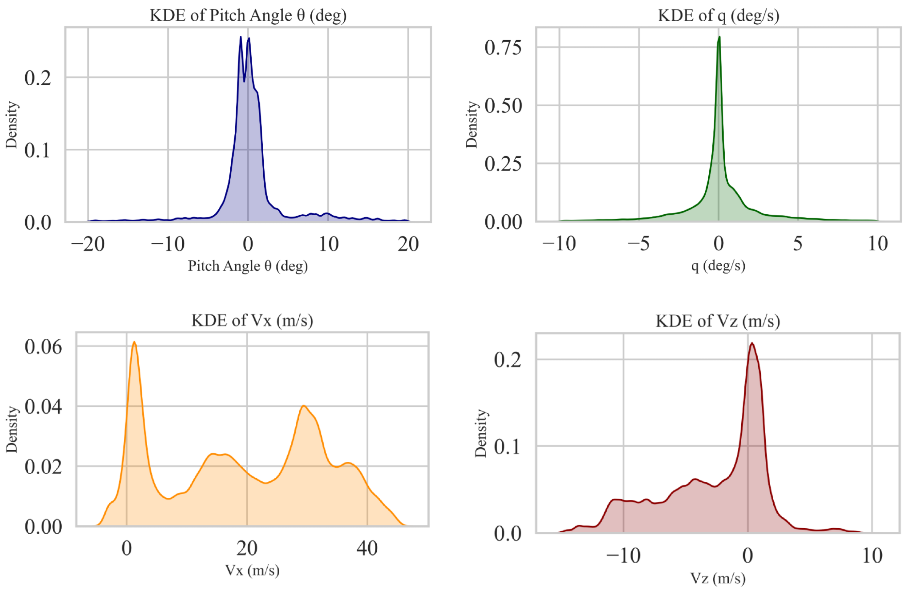
As shown in Figure 6, Kernel Density Estimation (KDE) is used to visualize the state distribution of the offline dataset. The dataset captures diverse flight conditions. Both $\theta$ and q are centered near zero, reflecting overall stability with minor perturbations. A negative peak in $\theta$ aligns with the nose-down stability observed in fixed-wing mode [40]. $V_x$ exhibits a multimodal pattern across hover, transition, and cruise phases. $V_z$ is near zero but skewed negative due to frequent descent scenarios, enabling the agent to recognize excessive altitude loss as risky. This distribution diversity ensures broad scenario coverage for training.

4. Proposed Approach

4.1. Problem Formulation

In this subsection, we present the mathematical formulation of the control objectives for the newly designed tilt-wing UAV throughout the entire flight process. The core requirement is to prevent large fluctuations in the pitch angle $\theta$ and to avoid significant descent in the vertical position z (flight altitude). The control objectives can be summarized as follows.

• Minimizing pitch angle deviation: $J_{\theta }={\int }_0^{t_f}{\theta }^{2}dt$
• Maintaining the pitch rate q near zero: $J_q={\int }_0^{t_f}{q}^{2}dt$
• Avoiding altitude changes: $J_z={\int }_0^{t_f}{(z_t-z_{ref})}^{2}dt$

The squared integral ensures nonnegativity, prevents error cancellation, and enhances convexity for easier optimization. It emphasizes larger deviations, improving stability, and captures cumulative effects for long-term performance while maintaining smoothness for gradient-based methods.

These objectives are incorporated into the offline reinforcement learning framework, where an optimal action policy is derived by searching the offline dataset for actions that effectively suppress pitch oscillations and minimize altitude loss. This ensures smooth and safe transitions throughout the mode-switching process of the UAV.

4.2. Algorithm Design and Implementation

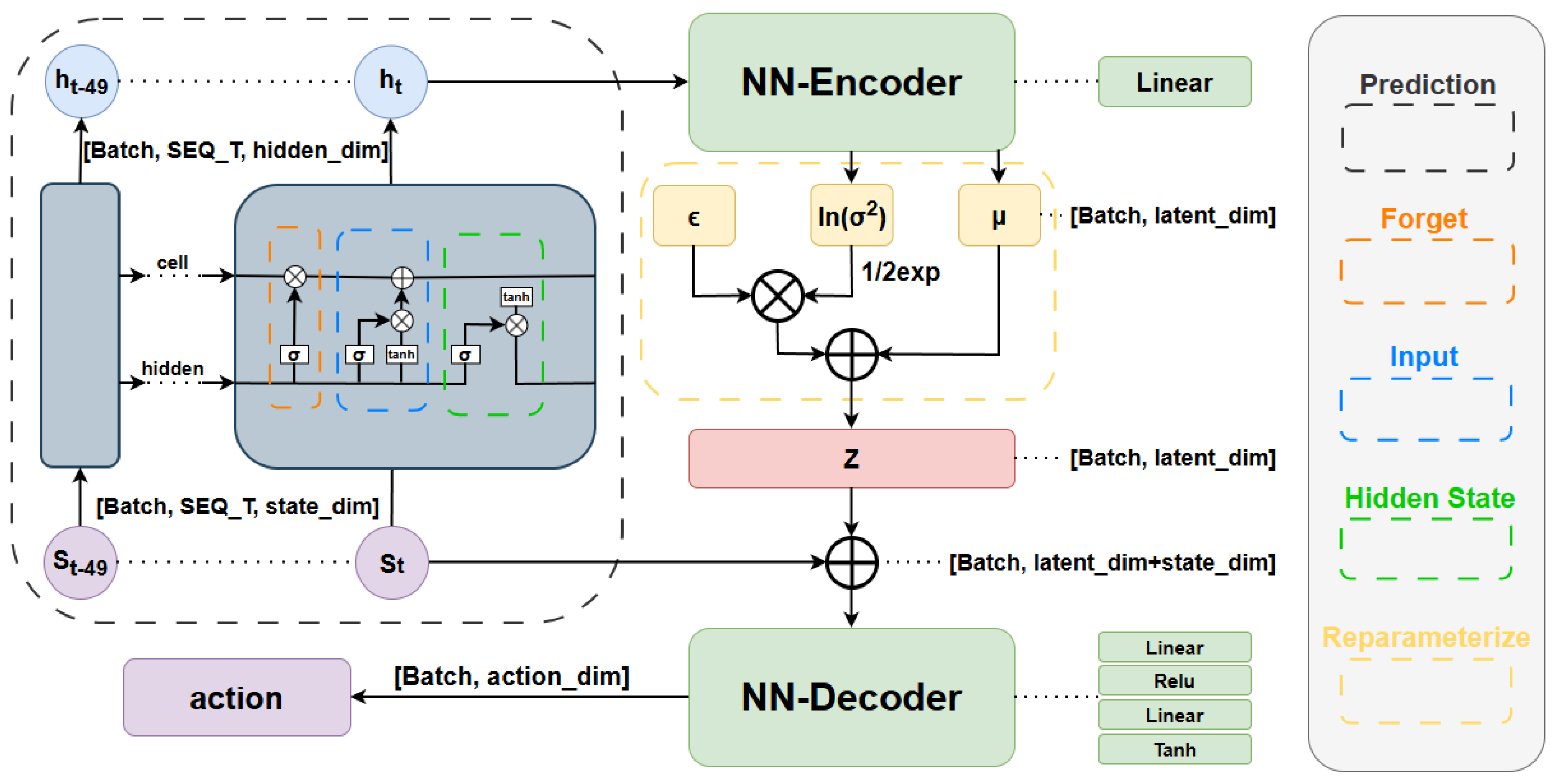
An unavoidable question in offline reinforcement learning algorithms is ‘balancing safety and exploration’. Traditional offline reinforcement learning algorithms, such as BCQ [41], CQL [42], and IQL [43], ensure policy safety by either penalizing deviations from the dataset policy or reducing the Q-values of unknown actions. Although certain techniques, such as small perturbations, allow for limited exploration, the lack of real-time interaction with the environment significantly restricts the effectiveness of exploration. The tilt-wing UAV studied in this work exhibits strong temporal dependencies in both state and action spaces. To address this, we propose Temporal Sequence Constrained Q-learning (TSCQ), an offline RL method for multi-phase flight control without real-world exploration. TSCQ combines temporal modeling with a variational autoencoder (VAE) to constrain the action space using offline data while capturing sequential patterns in flight dynamics. The generator architecture is illustrated in Figure 7.

The generator in TSCQ is trained using a VAE-based objective to ensure that the produced actions remain within the offline distribution. Unlike conventional VAE-based policies that take raw observations as input, TSCQ extracts a hidden representation h from the sequential data before passing it through the encoder. Specifically, given an input observation s, we first apply the long short-term memory network [44] (Equation (12)) to obtain the final hidden state h. This hidden state h then serves as the true input to the encoder.

$$\left\{\begin{array}{c}{f}_t=\sigma (W_f{S}_t+U_f{h}_{t-1}+b_f)\hfill \\ i_t=\sigma (W_i{S}_t+U_i{h}_{t-1}+b_i)\hfill \\ {\tilde{c}}_t=tanh(W_c{S}_t+U_c{h}_{t-1}+b_c)\hfill \\ c_t=f_t\odot c_{t-1}+i_t\odot {\tilde{c}}_t\hfill \\ o_t=\sigma (W_o{S}_t+U_o{h}_{t-1}+b_o)\hfill \\ h_t=o_t\odot tanh\left(c_t\right)\hfill \end{array}\right.$$

(12)

The current cell state $c_t$ is updated by the forget gate $f_t$, which regulates the contribution of the previous cell state $c_{t-1}$, and the input gate $i_t$, which controls the influence of the candidate cell state ${\tilde{c}}_t$. The updated cell state then modulates the output gate $o_t$ to generate the hidden state $h_t$.

$\sigma$ represents the Sigmoid activation function; $W_f,W_i,W_c$ represents the weight matrix of each gating mechanism for the current state; $U_f,U_i,U_c$ represents the weight matrix for the hidden state from the previous time step; $b_f,b_i,b_c$ is the bias term; and ⊙ represents element-wise multiplication.

From h, the encoder generates the mean $\mu$ and log-variance $log{\sigma }^2$ of a latent variable z, where $\mu$ and $\sigma$ are obtained by mapping h through a fully connected layer, and z is derived using the reparameterization trick:

$$z=\mu \left(h\right)+ϵ\sigma \left(h\right),ϵ\sim \mathcal{N}(0,\mathbf{I})$$

(13)

Finally, the decoder receives both s and z, concatenates them, and generates the reconstructed action $\tilde{a}$:

$$\tilde{a}=\mathrm{Decoder}\left([s,z]\right)$$

(14)

Since the decoder output passes through a tanh activation, the reconstructed actions are naturally constrained within a valid range. The generator is optimized using the following loss function, as shown in Equations (15) and (16).

$$L_{\mathrm{gen}}=\underset{\mathrm{Reconstruction}\mathrm{Loss}}{\underbrace{{∥\tilde{a}-a∥}^2}}+\underset{\mathrm{KL}\mathrm{Term}}{\underbrace{D_{\mathrm{KL}}\left(q(z\mid h)\parallel p\left(z\right)\right)}}-\underset{\mathrm{Q}\mathrm{Value}}{\underbrace{Q(s,\tilde{a})}}$$

(15)

$${\nabla }_{\theta }{D}_{\mathrm{KL}}(q(z\mid h)\parallel p\left(z\right))={\nabla }_{\theta }\left[-{\displaystyle \frac{1}{2}}{\displaystyle \sum _{i=1}^d}\left(1+log{\sigma }_i^2-{\mu }_i^2-{\sigma }_i^2\right)\right]$$

(16)

The reconstruction loss term constrains the decoder by minimizing the error between the predicted control action $\tilde{a}$ generated from the high-dimensional latent space z and the actual control action of the UAV a. This ensures that the generated control policy is both realistic and executable. The KL term constrains the encoder by ensuring that the learned latent variable distribution $q(z\mid h)$ remains close to the standard normal distribution $p\left(z\right)=N(0,\mathbf{I})$. This acts as a regularization mechanism, adjusting the mapping of h to the high-dimensional space z by the temporal extractor, ensuring it follows a standard normal distribution. Additionally, it prevents the learned representation from deviating significantly even in the presence of out-of-distribution (OOD) [45,46] state data, reducing the probability of generating latent representations outside the training distribution. The Q-value term is explicitly incorporated into the generator’s loss function, which enhances its ability to predict future states and improves control performance to a certain extent. As a result, it ensures a certain level of predictive generalization while minimizing the likelihood that the decoder generates unrealistic or infeasible control actions.

Similar to the generator, the Q-network in TSCQ does not directly take raw states and actions as inputs. Instead, given a pair of state actions $(s,a)$, the critic extracts the final hidden state h from the sequential processing layer. We define this relationship as $h(s,a)$. The final hidden representation h is then mapped to a scalar Q-value. The critic is trained via a Bellman backup objective, where the target value is computed using the maximum Q-value among candidate actions generated by the VAE-based policy, as shown in Equation (17):

$$L_{\mathrm{critic}}={∥Q_{{\theta }_q}\left(h(s,a)\right)-\left(r+\gamma \underset{a^{\prime }\in \mathcal{A}\left(s^{\prime }\right)}{max}{Q}_{{\theta }_q^{*}}\left(h^{\prime }(s^{\prime },a^{\prime })\right)\right)∥}^2$$

(17)

$${\theta }_q^{*}\leftarrow \tau {\theta }_q+(1-\tau ){\theta }_q^{*}$$

(18)

where ${\theta }_q$ and ${\theta }_q^{*}$ denote parameters of the current and target critic, respectively, and $\gamma$ is a discount factor. The key difference from standard offline Q-learning is that ${max}_{a^{\prime }}{Q}_{{\theta }_q^{*}}$ is computed over several reconstructed actions sampled from the generator. Each training iteration consists of a critic update and a delayed generator update, following a soft update strategy. Ultimately, TSCQ performs inference by generating candidate actions and selecting the one with the highest Q-value, as shown in Equation (19).

$$a^{*}=arg\underset{a\in \{{\tilde{a}}_1,\dots ,{\tilde{a}}_K\}}{max}{Q}_{{\theta }_q^{*}}\left(h(s,a)\right)$$

(19)

After network training is completed, the generator network and critic network need to be reconstructed during the testing phase. Once the network parameter dictionary is loaded, the trained model is used to output the optimal action $a^{*}$ corresponding to the current state. The main hyperparameters of the neural network are shown in

Table 1. The main hyperparameters of neural networks.

Hyperparameter	Value	Hyperparameter	Value
GENERATOR_LR	5 × 10−5	BATCH_SIZE	64
CRITIC_LR	5× 10−4	EPOCHS	100
MSE_WEIGHT	1.0	HIDDEN_DIM	256
KL_WEIGHT	1.0	LATENT_DIM	128
Q_VALUE_COEF 1	0.1	TAU	0.005
ACTION_LIMIT	1.0	GAMMA	0.99
POLICY_DELAY	2.0	$K_p$	1.0
SEQ_T 2	50.0	$K_z$	0.3

¹ This term represents the weight of the Q-value in the generator’s loss function. ² The number of time steps input for the temporal sequence module.

.

5. Experimental Evaluation

In this section, we provide a detailed description of the simulation experiments and the corresponding results. The specific experiments are outlined as follows.

• We set up an ablation study to validate the effectiveness of the temporal sequence module. We compare the TSCQ approach with BCQ, which also uses the VAE module, through ablation experiments.
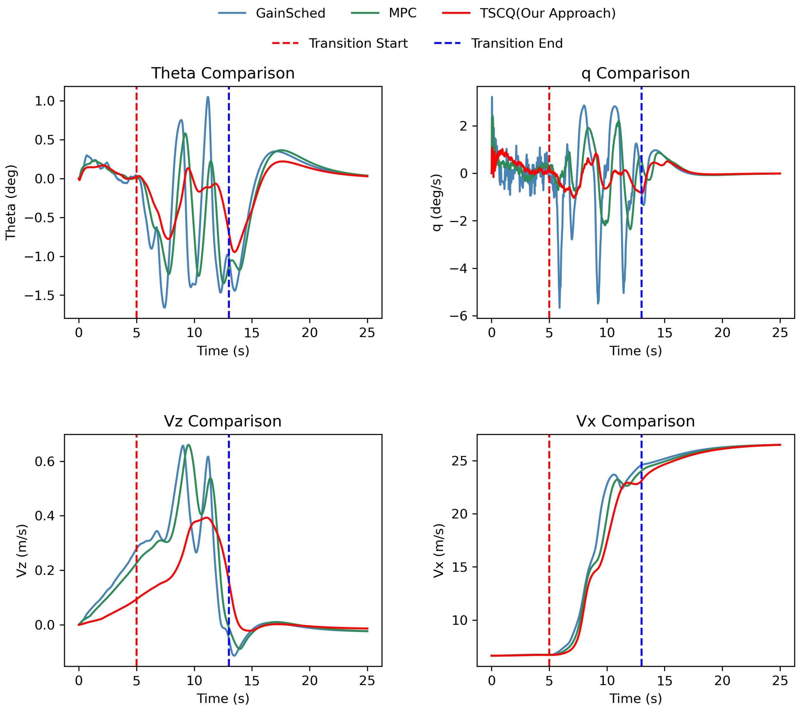
• Three controllers (gain scheduling, MPC, and TSCQ) are set up to compare the control performance of the newly designed tilt-wing UAV during the entire transition process from rotary-wing mode to the transition state and then to fixed-wing mode. The experimental results are presented as curves showing the variation over time of the pitch angle $\theta$, the pitch rate q, the vertical speed $V_z$, and the forward speed $V_x$.
• We perform robustness experiments on the TSCQ approach. To satisfy Monte Carlo experiments, we run 300 trials for each experiment group, where the initial conditions are altered or random perturbations are introduced.

5.1. Ablation Study and Analysis

The ablation experiment of TSCQ and BCQ (no temporal sequence prediction) highlights the crucial role of temporal prediction in enhancing control performance with temporal information. As shown in Figure 8, TSCQ, by integrating temporal sequence information, demonstrates proactive control behavior, which is absent in BCQ. Around the 11th second of the flight, TSCQ anticipates a downward trend in $\theta$, allowing it to suppress the trend in advance and reduce errors. This anticipatory behavior is more evident in the q plot, where TSCQ maintains smoother angular velocity and avoids abrupt spikes, whereas BCQ suffers from irregular control bursts, leading to angular instability. Specifically, BCQ experiences oscillations in $\theta$ and q, reaching ±2° and ±3°/s, respectively, while TSCQ limits these deviations to approximately ±0.8° and ±1°/s. Lacking temporal foresight, BCQ generates motor and control surface outputs only after state deviations occur, resulting in delayed correction and reduced stability. In contrast, around 5 and 10 s, the TSCQ Temporal Sequence Prediction architecture enables it to model the evolution of system states and implement feedforward control, allowing it to generate more effective actions in advance. This leads to a smoother and more robust transition process. This ablation confirms that the integration of the temporal sequence modeling is essential to accurately model transition dynamics. BCQ primarily constrains the distribution of single-step actions to avoid extrapolation beyond the offline dataset. In contrast, TSCQ introduces an additional prediction mechanism to ensure the consistency of entire action sequences, thereby further reducing the likelihood of generating OOD data.

5.2. Comparison Experiment

As shown in Figure 9, the comparison between TSCQ, gain scheduling, and MPC demonstrates that TSCQ offers significant advantages in controlling. During the transition phase, both gain scheduling and MPC exhibit substantial fluctuations in the pitch angle ($\theta$), with deviations reaching ±1.5°. Gain scheduling fails to effectively suppress dynamic responses. Although MPC shows slight improvement, it still exhibits pronounced high-frequency oscillations during the transition phase. This indicates that, despite its predictive capability, MPC performs poorly in handling rapidly changing nonlinear dynamics and suffers from slow computational speed. In contrast, TSCQ successfully maintains the pitch angle close to zero. Additionally, for the pitch rate (q), gain scheduling and MPC still experience significant oscillations after the transition begins, with values reaching ±6°/s, while TSCQ effectively minimizes the amplitude of q, stabilizing it close to zero throughout the entire flight phase.

Furthermore, the comparison of vertical speed ($V_z$) highlights the superior performance of TSCQ in minimizing vertical deviations. TSCQ exhibits considerably smaller fluctuations compared to gain scheduling and MPC, maintaining variations below 0.4 m/s. This enables TSCQ to provide smoother altitude control, ensuring that the aircraft avoids overshoot or excessive vertical motion during the transition.

In the comparison of forward velocity ($V_x$), all three control strategies, GAIN scheduling, MPC, and TSCQ, exhibit similar behavior during and after the transition. Following the initiation of transition (around 5 s), the aircraft pitches downward and accelerates, resulting in a clear increase in $V_x$. This reflects the conversion of vertical thrust into horizontal propulsion as the vehicle shifts from hover to fixed-wing flight. All controllers reach a comparable final forward velocity of approximately 25 m/s in fixed-wing mode, indicating successful completion of the transition in terms of horizontal acceleration. The similarity in $V_x$ trajectories suggests that, while TSCQ significantly improves pitch and vertical velocity control, forward acceleration dynamics are primarily influenced by the vehicle’s aerodynamics [47] and transition profile rather than the control strategy itself.

As shown in Figure 10, to provide a more intuitive comparison of control performance, we use the RMSE metric. Both gain scheduling and MPC exhibit a significant increase in $\theta$ RMSE during the transition phase, indicating large deviations from the set point and resulting in error accumulation. In contrast, TSCQ shows a much smaller increase in $\theta$ RMSE, with a notable decrease and fluctuation between 8 and 13 s, indicating that TSCQ adjusts the control actions earlier and more effectively than the other methods. Similarly, both gain scheduling and MPC experience large fluctuations in q RMSE during the transition, while TSCQ’s RMSE significantly drops to approximately 0.25, much lower than the other two methods. This sharp decrease reflects TSCQ’s ability to adjust control actions more effectively through proactive prediction, mitigating oscillations in q. In general, TSCQ outperforms traditional approaches in terms of control accuracy and stability, particularly in the control of key flight parameters such as $\theta$, q, and $V_z$.

5.3. Monte Carlo Experiments

To assess the robustness of TSCQ under real-world uncertainties, Monte Carlo simulations are conducted across four representative perturbation scenarios: transition time variation, sensor noise, motor degradation, and lift/drag disturbances. For each case, 300 randomized trials are performed with disturbances sampled from uniform distributions, whose ranges are based on physically realistic error margins. The results report the mean and 95% confidence intervals of four key metrics: maximum pitch error (${\theta }_{max}$), final pitch error (${\theta }_{final}$), maximum vertical speed error ($V_{z,max}$), and final vertical speed error ($V_{z,final}$). Detailed perturbation settings and success rates are summarized in

Table 2. Different perturbations and success rates.

Perturbation Type	Parameter	Success Rate
Transition time variation	8–11 s 1	96.67%
Sensor noise	5% Perturbation 2	94.67%
Motor Degradation	5% Perturbation 2	99.00%
Lift/drag perturbation	10% Perturbation 3	94.00%

¹ The transition time is randomly selected between 8 and 11 s. ² The experiment uses a typical measurement sensor error range of 5%. ³ A 10% deviation provides a well-controlled and sufficiently significant bias.

.

As shown in Figure 11, the TSCQ controller demonstrates exceptional robustness across all perturbation types. Notably, all metrics under perturbation remain close to their nominal (no perturbation) performance levels. For example, ${\theta }_{max}$ remains within 1.0°–1.2°, compared to the nominal value of around 1.0°, while $V_{z,max}$ remains between 0.387 and 0.422 m/s, almost identical to the nominal performance. Similarly, final errors are exceptionally small and stable: ${\theta }_{final}$ ranges from 0.028° to 0.058°, and $V_{z,final}$ stays within 0.012–0.014 m/s. This consistency indicates that TSCQ maintains both transient and steady-state accuracy despite external perturbations. The short confidence intervals, indicated by the vertical bars, reflect low variance and high reliability of the controller. This consistency across trials suggests that TSCQ achieves not only strong average performance but also robust repeatability—an essential trait for real-world deployment.

When individual perturbations are broken down, distinct characteristics emerge:

• Transition time variation introduces the largest transient error, with the highest ${\theta }_{max}$ (1.236°) and ${\theta }_{final}$ (0.058°). This reflects the challenge of adapting to uncertain switching moments between flight modes. Despite this, the final vertical error remains minimal (0.012 m/s), showing strong recovery in altitude tracking.
• Sensor Noise causes moderate error across all metrics. The confidence intervals here are slightly wider, particularly for ${\theta }_{final}$, suggesting higher sensitivity from trial to trial. This is likely due to measurement fluctuations that introduce irregular feedback delays.
• Motor degradation produces the highest vertical deviation during transition $V_{z,max}$ (0.422 m/s), likely caused by asymmetric thrust distribution. However, attitude errors remain tightly bounded, indicating that the controller compensates well through attitude correction.
• Lift/drag perturbation results in the lowest errors overall, with ${\theta }_{max}$ (1.007°) and ${\theta }_{final}$ (0.028°), along with narrow confidence intervals across all metrics. This suggests that the aerodynamic model effectively absorbs such variations, making them the least disruptive among the four.

The Monte Carlo experiments provide strong empirical evidence of the robustness and safety of the proposed TSCQ algorithm. Under diverse perturbations in initial conditions—such as speed, pitch angle, and tilt progression—TSCQ consistently maintains low variance in pitch angle and vertical velocity, demonstrating resilience to both state uncertainty and modeling errors. Beyond empirical validation, the algorithm’s architecture further enhances safety: the sequence-level consistency constraint ensures smooth, non-oscillatory control over long horizons, while the VAE-based regularization limits policy inference to high-confidence regions in the offline dataset. These two mechanisms jointly mitigate extrapolation risk and unstable action generation. Compared to conventional offline RL methods such as BCQ that constrain actions only at the individual step level, TSCQ enforces structural regularization across temporal sequences by modeling inter-step action dependencies, thereby exhibiting greater stability and generalization under dynamically uncertain environments.

6. Conclusions and Discussion

In this study, we (i) formulated a high-fidelity mathematical model for a newly designed tilt-wing UAV, capturing the wing-tilting kinematics with rotation matrices; (ii) adapted the on-board control logic and executed hardware-in-the-loop simulations on a real-time computer to build a large, diversity-enhanced offline data set; and (iii) introduced Temporal Sequence Constrained Q-learning (TSCQ), an offline RL algorithm that simultaneously regulates longitudinal attitude and vertical velocity throughout rotary-wing, transition, and fixed-wing modes. Extensive comparative, ablation, and Monte Carlo experiments verify the superiority, validity, and robustness of TSCQ. The results show that its temporal-prediction module is essential for tasks with strong temporal dependencies, lowering the pitch-angle RMSE by 53.3% and the vertical velocity RMSE by 33% relative to baseline controllers. These gains are enabled by the comprehensive offline data set, expert-guided refinement, and the recurrent encoder–decoder architecture, which together ensure strict consistency between input states and generated actions.

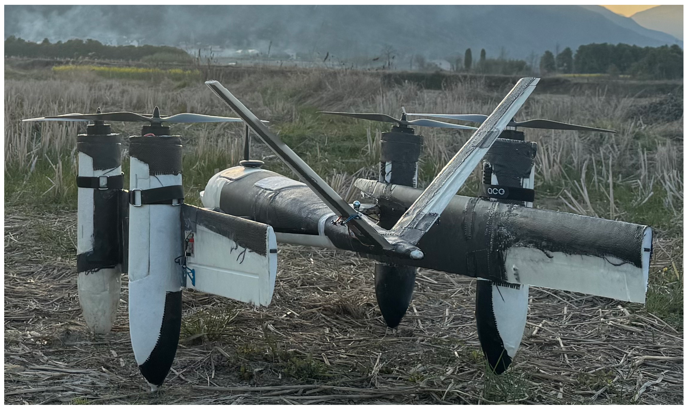
As shown in Figure 12, other members of the project team have completed a prototype of the newly designed tilt-wing UAV and successfully conducted full-transition flight tests based on a gain scheduling strategy. The prototype serves as the physical foundation for the modeling work in Section 2. Wind tunnel experiments on this airframe provided the aerodynamic coefficients for the five representative tilt configurations. In addition, geometric parameters such as moment arms, rotor positions, and center-of-gravity offsets used in the model were derived from its CAD design and mass distribution. Future research will focus on optimizing the neural network architecture for real-time deployment, with plans to implement the algorithm on the physical platform to comprehensively evaluate its feasibility and robustness in real-world flight missions.

References

1. Misra, A.; Jayachandran, S.; Kenche, S.; Katoch, A.; Suresh, A.; Gundabattini, E.; Selvaraj, S.K.; Legesse, A.A. A Review on Vertical Take-Off and Landing (VTOL) Tilt-Rotor and Tilt Wing Unmanned Aerial Vehicles (UAVs). J. Eng. 2022, 2022, 1803638. [Google Scholar] [CrossRef]
2. Autenrieb, J.; Shin, H.S. Complementary Filter-Based Incremental Nonlinear Model Following Control Design for a Tilt-Wing UAV. Int. J. Robust Nonlinear Control 2025, 35, 1596–1615. [Google Scholar] [CrossRef]
3. Çetinsoy, E.; Dikyar, S.; Hançer, C.; Oner, K.; Sirimoglu, E.; Unel, M.; Aksit, M. Design and construction of a novel quad tilt-wing UAV. Mechatronics 2012, 22, 723–745. [Google Scholar] [CrossRef]
4. Erbil, M.A.; Prior, S.D.; Karamanoglu, M.; Odedra, S.; Barlow, C.; Lewis, D. Reconfigurable Unmanned Aerial Vehicles; 2009. Available online: https://eprints.soton.ac.uk/343526/1/Erbil%252C_M.A._Reconfigurable_Unmanned_Aerial_Vehicles_MES2009356.pdf (accessed on 11 May 2025).
5. Huang, Q.; He, G.; Jia, J.; Hong, Z.; Yu, F. Numerical simulation on aerodynamic characteristics of transition section of tilt-wing aircraft. Aerospace 2024, 11, 283. [Google Scholar] [CrossRef]
6. Rojo-Rodriguez, E.U.; Rojo-Rodriguez, E.G.; Araujo-Estrada, S.A.; Garcia-Salazar, O. Design and performance of a novel tapered wing tiltrotor UAV for hover and cruise missions. Machines 2024, 12, 653. [Google Scholar] [CrossRef]
7. Whiteside, S.K.; Pollard, B.P.; Antcliff, K.R.; Zawodny, N.S.; Fei, X.; Silva, C.; Medina, G.L. Design of a Tiltwing Concept Vehicle for Urban Air Mobility; Technical Report; NASA: Washington, DC, USA, 2021.
8. May, M.S.; Milz, D.; Looye, G. Transition Strategies for Tilt-Wing Aircraft. In Proceedings of the AIAA SciTech 2024 Forum, Orlando, FL, USA, 8–12 January 2024; p. 1289. [Google Scholar]
9. Fatemi, M.M. Optimized Sliding Mode Control via Genetic Algorithm for Quad Tilt-Wing UAVs. In Proceedings of the 2024 10th International Conference on Artificial Intelligence and Robotics (QICAR), Qazvin, Iran, 29 February 2024; pp. 281–285. [Google Scholar]
10. Dickeson, J.J.; Cifdaloz, O.; Miles, D.W.; Koziol, P.M.; Wells, V.L.; Rodriguez, A.A. Robust H gain-scheduled conversion for a tilt-wing rotorcraft. In Proceedings of the 45th IEEE Conference on Decision and Control, San Diego, CA, USA, 13–15 December 2006; pp. 5882–5887. [Google Scholar]
11. Benkhoud, K.; Bouallègue, S. Model predictive control design for a convertible quad tilt-wing UAV. In Proceedings of the 2016 4th International Conference on Control Engineering & Information Technology (CEIT), Hammamet, Tunisia, 16–18 December 2016; pp. 1–6. [Google Scholar]
12. Yoo, C.S.; Ryu, S.D.; Park, B.J.; Kang, Y.S.; Jung, S.B. Actuator controller based on fuzzy sliding mode control of tilt rotor unmanned aerial vehicle. Int. J. Control. Autom. Syst. 2014, 12, 1257–1265. [Google Scholar] [CrossRef]
13. Masuda, K.; Uchiyama, K. Robust control design for quad tilt-wing UAV. Aerospace 2018, 5, 17. [Google Scholar] [CrossRef]
14. Yang, R.; Du, C.; Zheng, Y.; Gao, H.; Wu, Y.; Fang, T. PPO-based attitude controller design for a tilt rotor UAV in transition process. Drones 2023, 7, 499. [Google Scholar] [CrossRef]
15. Akhtar, M.; Maqsood, A. Comparative Analysis of Deep Reinforcement Learning Algorithms for Hover-to-Cruise Transition Maneuvers of a Tilt-Rotor Unmanned Aerial Vehicle. Aerospace 2024, 11, 1040. [Google Scholar] [CrossRef]
16. Guo, H.; Li, F.; Li, J.; Liu, H. Offline Reinforcement Learning via Conservative Smoothing and Dynamics Controlling. In Proceedings of the ICASSP 2025–2025 IEEE International Conference on Acoustics, Speech and Signal Processing (ICASSP), Hyderabad, India, 6–11 April 2025; pp. 1–5. [Google Scholar]
17. Feng, Y.; Hansen, N.; Xiong, Z.; Rajagopalan, C.; Wang, X. Finetuning offline world models in the real world. arXiv 2023, arXiv:2310.16029. [Google Scholar]
18. Xu, H.; Jiang, L.; Li, J.; Yang, Z.; Wang, Z.; Chan, V.W.K.; Zhan, X. Offline rl with no ood actions: In-sample learning via implicit value regularization. arXiv 2023, arXiv:2303.15810. [Google Scholar]
19. Liu, J.; Zhang, Z.; Wei, Z.; Zhuang, Z.; Kang, Y.; Gai, S.; Wang, D. Beyond ood state actions: Supported cross-domain offline reinforcement learning. In Proceedings of the AAAI Conference on Artificial Intelligence, Philadelphia, PA, USA, 25 February–4 March 2024; Volume 38, pp. 13945–13953. [Google Scholar]
20. Sato, M.; Muraoka, K. Flight controller design and demonstration of quad-tilt-wing unmanned aerial vehicle. J. Guid. Control. Dyn. 2015, 38, 1071–1082. [Google Scholar] [CrossRef]
21. Totoki, H.; Ochi, Y.; Sato, M.; Muraoka, K. Design and testing of a low-order flight control system for quad-tilt-wing UAV. J. Guid. Control. Dyn. 2016, 39, 2426–2433. [Google Scholar] [CrossRef]
22. Sherstinsky, A. Fundamentals of recurrent neural network (RNN) and long short-term memory (LSTM) network. Phys. D Nonlinear Phenom. 2020, 404, 132306. [Google Scholar] [CrossRef]
23. Dai, B.; Wipf, D. Diagnosing and enhancing VAE models. arXiv 2019, arXiv:1903.05789. [Google Scholar]
24. Holsten, J.; Ostermann, T.; Dobrev, Y.; Moormann, D. Model validation of a tiltwing UAV in transition phase applying windtunnel investigations. In Proceedings of the Congress of the International Council of the Aeronautical Sciences, International Council of the Aeronautical Sciences, Brisbane, Australia, 23–28 September 2012; Volume 28, pp. 1–10. [Google Scholar]
25. Rohr, D.; Studiger, M.; Stastny, T.; Lawrance, N.R.; Siegwart, R. Nonlinear model predictive velocity control of a VTOL tiltwing UAV. IEEE Robot. Autom. Lett. 2021, 6, 5776–5783. [Google Scholar] [CrossRef]
26. Mulder, J.; Chu, Q.; Sridhar, J.; Breeman, J.; Laban, M. Non-linear aircraft flight path reconstruction review and new advances. Prog. Aerosp. Sci. 1999, 35, 673–726. [Google Scholar] [CrossRef]
27. Luukkonen, T. Modelling and control of quadcopter. Indep. Res. Proj. Appl. Math. 2011, 22, 1–24. [Google Scholar]
28. Abdulghany, A. Generalization of parallel axis theorem for rotational inertia. Am. J. Phys. 2017, 85, 791–795. [Google Scholar] [CrossRef]
29. Poksawat, P.; Wang, L.; Mohamed, A. Gain scheduled attitude control of fixed-wing UAV with automatic controller tuning. IEEE Trans. Control Syst. Technol. 2017, 26, 1192–1203. [Google Scholar] [CrossRef]
30. Mathisen, S.H.; Fossen, T.I.; Johansen, T.A. Non-linear model predictive control for guidance of a fixed-wing UAV in precision deep stall landing. In Proceedings of the 2015 International Conference on Unmanned Aircraft Systems (ICUAS), Denver, CO, USA, 9–12 June 2015; pp. 356–365. [Google Scholar]
31. Saderla, S.; Rajaram, D.; Ghosh, A. Parameter estimation of unmanned flight vehicle using wind tunnel testing and real flight data. J. Aerosp. Eng. 2017, 30, 04016078. [Google Scholar] [CrossRef]
32. Thacker, B.H.; Doebling, S.W.; Hemez, F.M.; Anderson, M.C.; Pepin, J.E.; Rodriguez, E.A. Concepts of Model Verification and Validation 2004. Available online: https://inis.iaea.org/records/egfyy-d4t03 (accessed on 11 May 2025).
33. Prudencio, R.F.; Maximo, M.R.; Colombini, E.L. A survey on offline reinforcement learning: Taxonomy, review, and open problems. IEEE Trans. Neural Netw. Learn. Syst. 2023, 35, 10237–10257. [Google Scholar] [CrossRef] [PubMed]
34. Agarwal, R.; Schuurmans, D.; Norouzi, M. An optimistic perspective on offline reinforcement learning. In Proceedings of the International Conference on Machine Learning, Shenzhen, China, 15–17 February 2020; pp. 104–114. [Google Scholar]
35. Yao, Y.; Cen, Z.; Ding, W.; Lin, H.; Liu, S.; Zhang, T.; Yu, W.; Zhao, D. Oasis: Conditional distribution shaping for offline safe reinforcement learning. Adv. Neural Inf. Process. Syst. 2024, 37, 78451–78478. [Google Scholar]
36. Lu, W. Hardware-in-the-loop simulation test platform for UAV flight control system. Int. J. Model. Simul. Sci. Comput. 2024, 15, 2441018. [Google Scholar] [CrossRef]
37. Sotero, M.; Campos, B.F.d.A.; Silva, Í.S.S.; Mello, G.; Rolim, L.G.B. Hardware-in-the-Loop Modeling and Simulation of the Fin Control Subsystem with DSP. In Proceedings of the 2024 IEEE International Conference on Electrical Systems for Aircraft, Railway, Ship Propulsion and Road Vehicles & International Transportation Electrification Conference (ESARS-ITEC), Naples, Italy, 26–29 November 2024; pp. 1–6. [Google Scholar]
38. Santoso, F.; Garratt, M.A.; Anavatti, S.G.; Wang, J.; Tran, P.V.; Ferdaus, M.M. Bio-Inspired Adaptive Fuzzy Control Systems for Precise Low-Altitude Hovering of an Unmanned Aerial Vehicle Under Large Uncertainties. In Proceedings of the 2024 European Control Conference (ECC), Stockholm, Sweden, 25–28 June 2024; pp. 3777–3782. [Google Scholar]
39. Konyushkova, K.; Zolna, K.; Aytar, Y.; Novikov, A.; Reed, S.; Cabi, S.; de Freitas, N. Semi-supervised reward learning for offline reinforcement learning. arXiv 2020, arXiv:2012.06899. [Google Scholar]
40. Olcott, J.W.; Sackel, E.; Ellis, D.R. Analysis and Flight Evaluation of a Small, Fixed-Wing Aircraft Equipped with Hinged Plate Spoilers; Technical Report; NASA: Washington, DC, USA, 1981.
41. Fujimoto, S.; Meger, D.; Precup, D. Off-policy deep reinforcement learning without exploration. In Proceedings of the International Conference on Machine Learning, Long Beach, CA, USA, 9–15 June 2019; pp. 2052–2062. [Google Scholar]
42. Kumar, A.; Zhou, A.; Tucker, G.; Levine, S. Conservative Q-Learning for Offline Reinforcement Learning. In Proceedings of the Advances in Neural Information Processing Systems; Larochelle, H., Ranzato, M., Hadsell, R., Balcan, M., Lin, H., Eds.; Curran Associates, Inc.: Red Hook, NY, USA, 2020; Volume 33, pp. 1179–1191. [Google Scholar]
43. Kostrikov, I.; Nair, A.; Levine, S. Offline reinforcement learning with implicit q-learning. arXiv 2021, arXiv:2110.06169. [Google Scholar]
44. Hochreiter, S.; Schmidhuber, J. Long short-term memory. Neural Comput. 1997, 9, 1735–1780. [Google Scholar] [CrossRef]
45. Mao, Y.; Wang, Q.; Chen, C.; Qu, Y.; Ji, X. Offline reinforcement learning with ood state correction and ood action suppression. arXiv 2024, arXiv:2410.19400. [Google Scholar]
46. Cho, M.; How, J.P.; Sun, C. Out-of-distribution adaptation in offline rl: Counterfactual reasoning via causal normalizing flows. arXiv 2024, arXiv:2405.03892. [Google Scholar]
47. Yuksek, B.; Vuruskan, A.; Ozdemir, U.; Yukselen, M.; Inalhan, G. Transition flight modeling of a fixed-wing VTOL UAV. J. Intell. Robot. Syst. 2016, 84, 83–105. [Google Scholar] [CrossRef]
Figure 1. The transition process of the newly designed tilt-wing UAV. (a) Rotary-wing mode (b) Forward transition (c) Fixed-wing mode (d) Backward transition.
Aerospace 12 00435 g001
Figure 2. Definitions of the body-fixed and wing-fixed coordinate systems. In the body frame, the front-right and rear-left rotors spin counterclockwise, while the others spin clockwise. This configuration cancels net yaw torque, supporting symmetry assumptions in the torque model.
Aerospace 12 00435 g002
Figure 3. The definitions of the body-fixed coordinate system and the wing-fixed coordinate system.
Aerospace 12 00435 g003
Figure 4. The horizontal axis indicates the angle of attack α , and the vertical axes represent the lift coefficient C L and drag coefficient C D for different wing unfolding ratios K { 0 , 0.25 , 0.5 , 0.75 , 1 } .
Aerospace 12 00435 g004
Figure 5. Schematic diagram of the HIL simulation connection.
Aerospace 12 00435 g005
Figure 6. KDE for different states.
Aerospace 12 00435 g006
Figure 7. The generator network architecture of the TSCQ algorithm.
Aerospace 12 00435 g007
Figure 8. Comparison of experiments between BCQ and TSCQ.
Aerospace 12 00435 g008
Figure 9. Comparison of experiments between gain scheduling, MPC, and TSCQ.
Aerospace 12 00435 g009
Figure 10. RMSE metrics of gain scheduling, MPC, and TSCQ.
Aerospace 12 00435 g010
Figure 11. Monte Carlo experiments.
Aerospace 12 00435 g011
Figure 12. Physical prototype of the newly designed tilt-wing UAV.
Aerospace 12 00435 g012