Abstract
Path planning for stratospheric airships in dynamic wind fields is challenging due to complex wind variations and strict nighttime energy constraints. This paper proposes a hybrid Level-Set Particle Swarm Optimization (LS-PSO) framework. Firstly, it employs PSO to search iteratively for a propulsion velocity sequence in the velocity domain, with a multi-objective fitness function that integrates reachability, energy consumption and time cost to evaluate each velocity sequence. Then, the reachability of each candidate sequence is numerically solved by the Level Set forward evolution. To improve optimization efficiency, we proposed a multi-resolution grid adaptive strategy for forward evolutions. Finally, with the optimal velocity sequence, the optimal path is generated once by the Level Set backtrack processing. To validate the resulting methodology, we used a benchmark case of a dynamic complex four-gyre flow, described by mathematical formulas, with the optimal day–night path identified by GPOPS-II. The results show the LS-PSO solution has comparable accuracy, with a trajectory deviation less than 3%. Then, we tested the methodology in the stratospheric wind flows using ERA5 reanalysis data. The results demonstrate that our path planning methodology provides a computationally efficient and optimal energy–time solution for autonomous stratospheric airships, while conforming to reachability and strict nighttime energy constraints.
1. Introduction
As representative near-space vehicles, stratospheric airships operate at altitudes between 18.3 and 22.9 km within steady wind fields [1], effectively avoiding meteorological disturbances prevalent in the troposphere. Recent advancements in lightweight composite materials [2] and high-energy-density battery technologies [3] have significantly enhanced their payload capacity and energy efficiency, enabling continuous operation spanning weeks to months through coordinated solar-storage energy systems [4]. Leveraging their unique buoyancy–weight equilibrium design, these airships achieve long-duration steady flight at fixed altitudes without requiring energy expenditure for frequent altitude adjustments [5]. With wind field forecasting technology, its possible to dynamically optimize energy allocation and trajectory planning to maximize operational economics while ensuring mission reliability. These technological breakthroughs establish stratospheric airships as ideal platforms for extended-duration missions including atmospheric monitoring [6] and regional communication relays [7].
However, when executing long-endurance missions, the platform faces significant challenges from coupled flight environment and energy constraints. Although stratospheric winds demonstrate short-term stability at small scales, they exhibit pronounced latitudinal variations and diurnal fluctuations [8]. An airship’s low thrust-to-weight ratio and large wind-facing area result in cruise speeds comparable to background wind velocities, rendering trajectory planning highly sensitive to wind disturbances [7]. Furthermore, the inherent diurnal asymmetry of energy systems imposes critical operational constraints [9,10]—photovoltaic power generation sustains full propulsion and payload operations during daylight hours, while nighttime operations are strictly limited by finite battery storage capacity [11]. This energy supply imbalance causes dramatic reductions in nocturnal propulsion power, severely compromising the airship’s anti-drift capability in dynamic nighttime wind fields [12].
Current research on the exploration of stratospheric airships for cross-day-and-night missions primarily focuses on optimizing energy management strategies [13,14,15]. Approaches include enhancing wind resistance through high-power operation during the day and switching to low-power modes at night [9], or utilizing the surplus energy accumulated during the day to build positional potential energy to counteract nighttime drift [14]. Although these methods provide operational guidelines for day-and-night flight, a comprehensive theoretical system integrating the time-varying characteristics of energy with the dynamic evolution of wind fields has yet to be established. At the level of path planning, traditional algorithms (such as A* [16], APF [17], Dijkstra [18], and RRT [19]), despite their advancements in the field of robotics, struggle to adapt to the spatiotemporal dynamic characteristics of stratospheric wind fields due to their simplistic structures, and they generally lack a systematic integration of energy constraints [5,20]. Although deep reinforcement learning (DRL) methods (such as the PPO strategy by Liu et al. [5] and the DDQN model by Hou et al. [21]) demonstrate adaptability to dynamic environments, their decision-making processes largely rely on current wind speed, lacking a comprehensive consideration of future wind field changes, which results in trajectory planning that cannot balance energy efficiency with mission timeliness in long-term missions. Meta-heuristic algorithms (such as PSO [15], GA [22]), while possessing global optimization potential, are significantly limited in computational efficiency and adaptability in dynamic wind fields, making it difficult to support long-duration continuous mission requirements. The algorithms mentioned above struggle to deal with the complex coupling effects of spatiotemporal wind field variation and energy constraints [23].The fundamental flaw in existing studies lies in the separation of path planning and energy management, which makes it hard to achieve an optimal balance between mission success rate and energy efficiency under complex wind field variation and strict energy limitations [15]. Such negligence may lead to catastrophic operational failures: in nocturnal phases with depleted energy reserves, airships could lose propulsion control under dynamic wind disturbances, potentially drifting into restricted airspace or suffering irreversible battery damage due to deep discharge cycles.
Consequently, the core issue of cross-day-and-night planning for stratospheric airships remains unresolved: given wind field predictions and nighttime energy consumption constraints, how can one construct a reliable path planning method to achieve a dynamic balance between mission execution efficiency and system survivability? In response to this challenge, there is an urgent need to develop a new path planning framework.
The level-set method (LSM), initially proposed by Lolla et al. [24], established a theoretical scheme for the reachability analysis and trajectory optimization in dynamic environments through the solution of Hamilton–Jacobi partial differential equations. Its core advantage lies in the ability to integrate environmental forecast data, generating adaptive planning strategies based on spatiotemporal flow field characteristics. This enables vehicles to achieve efficient path planning in fluid environments by actively leveraging favorable flow fields while avoiding adverse ones [24]. The LSM scheme workflow comprises two phases: firstly, the method performs the forward evolution with the given velocity to propagate the front of the reachable set, followed by obtaining optimal paths and heading sequences via the backward tracing from target locations. Existing studies demonstrate the method’s significant engineering value in time-varying flows, such as oceanic current path planning [25,26]. However, traditional LSM implementations critically depend on static velocity assumptions—preset speed parameters lack dynamic adaptation mechanisms to accommodate either closed-loop energy constraint feedback or time-varying speed adjustment requirements in cross-day–night missions, fundamentally limiting their applicability to stratospheric airship operations [27,28,29].
To address these challenges, we propose a novel hybrid planning framework that integrates the LSM with particle swarm optimization through hierarchical coordination. The framework features a dual-phase optimization architecture: The first phase employs dynamic velocity domain exploration coupled with reachability analysis to ensure path feasibility while incorporating energy constraints. This is achieved through iterative feedback between velocity optimization and trajectory validation. The second phase constructs energy-compliant trajectories via the backward tracing, utilizing the optimized velocity parameters. This hierarchical integration maintains the LSM’s rigorous dynamic wind field modeling capabilities while leveraging PSO’s global optimization strength to resolve complex energy constraints, ultimately delivering an environment-responsive and operationally viable solution for stratospheric airship missions spanning diurnal cycles.
This paper is organized as follows. Section 2 establishes the path planning problem for solar-powered stratospheric airships operating in dynamic wind flows under diurnal energy constraints. This includes the formal problem formulation, kinematic and energy consumption models, as well as the associated operational constraints. Section 3 introduces the proposed Level Set-Particle Swarm Optimization (LS-PSO) methodology, detailing the integration of Hamilton–Jacobi reachability analysis with particle swarm optimization for velocity sequence optimization and constrained path generation. Section 4 presents experimental validation of the LS-PSO framework through benchmark comparisons against pseudospectral optimization in controlled synthetic wind fields and operational testing using ERA5 reanalysis data. These experiments evaluate the algorithm’s ability to balance energy efficiency and mission duration while adhering to nighttime energy constraints. Finally, Section 5 discusses the contributions of this study, highlights the practical implications for stratospheric airship path planning, and outlines potential future research.
2. Problem Formulation
For the path planning of a stratospheric airship, it is assumed that the airship flies at a fixed altitude, treated as a particle. As illustrated in Figure 1, on a 2-D plane, an airship is tasked with flying from an initial position to a target position . The body-fixed coordinate system is established in the earth-fixed coordinate system . Let denote the magnitude of the airship’s propulsion speed relative to the wind field and let the unit vector represent the direction vector of, i.e., the heading direction of the airship. Its motion is influenced by the time-varying stratospheric wind field . represents the velocity of the airship under the influence of the wind, as observed from the ground. The motion of the airship can therefore be modeled by the following equations of motion [24]:
where the wind field is known. Subject to propulsion limitations, the airspeed is constrained within the range .
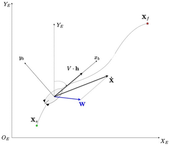
Figure 1.
Coordinate systems and velocity components for airship motion modeling in dynamic wind fields.
The energy consumption primarily considers the propulsion system’s power requirements and is usually modeled as a cubic function of airspeed in airship problems [11,30,31]. The energy consumption models are given as follows:
where is a coefficient determined by propulsion efficiency. During the mission duration , the total energy consumed by the airship for propulsion is while the total energy consumed during the nocturnal period is , as detailed in Equation (4). Here, we assume that the maximum energy an airship can convert into thrust during the nocturnal hours does not exceed .
The objective is to determine an optimal path that minimizes energy consumption or travel time while satisfying energy and operational constraints. This path planning problem can be formulated as a constrained multi-objective optimization problem:
subject to
3. Methodology
To tackle the multi-constraint challenges of cross-day-and-night path planning, we propose an integrated Level-Set Particle Swarm Optimization (LS-PSO) framework. We treat the propulsion velocity sequence as the optimization variable. As illustrated in Figure 2, the reachable set denotes all positions attainable by time with the propulsion speed profile under wind field . The reachable set front is defined as the boundary of . The velocity along the normal direction of the reachable front enables the fastest propagation of the reachable set under the background flow field .
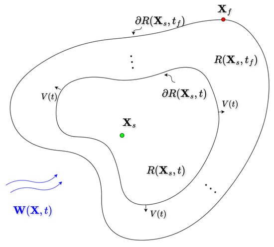
Figure 2.
Illustration of reachable set evolution with propulsion speed V(t) under wind field W(X,t).
When the reachable set front expands to the target position within the maximum allowable time, the path is deemed reachable. Subsequently, by evolving backward from along the normal direction of the reachable front, the optimal efficiency trajectory with the propulsion velocity profile under the flow field can be determined. In this way, the path planning problem introduced in Section 2 is transformed into a velocity profile optimization problem:
subject to:
To solve this optimization problem efficiently, a two-stage hybrid framework (as illustrated in Figure 3) is adopted, integrating Hamilton–Jacobi reachability analysis with metaheuristic search using a time-discretized model.
- Velocity Sequence Optimization and feasibility verification: we use PSO to search for candidate velocities in the velocity domain and adopt the level-set method to evolve the reachable set in the wind field to validate path reachability. The level-set evolution results are used to quantify energy consumption, arrival time, and constraint violations, guiding the fitness evaluation of the particle swarm. Through iterative optimization, the method identifies an optimal velocity sequence that satisfies nighttime energy constraints while minimizing propulsion energy consumption. A detailed explanation is shown in Section 3.1.
- Optimal path generation: With the optimized velocity sequence, the final space-domain path is computed using the backward evolution of the LSM. Further details are described in Section 3.2.
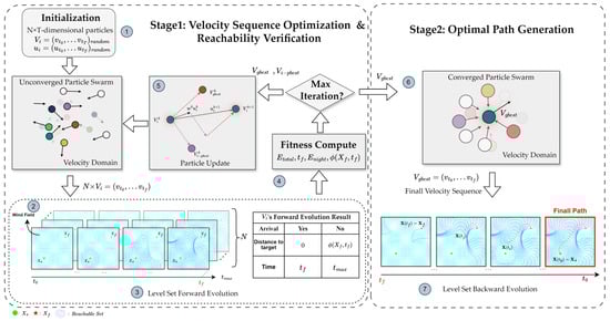
Figure 3.
LS-PSO framework.
3.1. Velocity Sequence Optimization and Reachability Verification
The first stage iteratively refines velocity sequences using an integration of PSO and level-set forward evolution. Each particle in the particle swarm encodes a candidate velocity sequence , representing propulsion speeds at a discrete time step, and satisfies the maximum propulsion speed constraint of the airship by restricting the particle’s motion range to . For every candidate sequence, the level-set method propagates a signed distance function governed by the Hamilton–Jacobi partial differential equation [24]:
where the level set function is initialized as a signed distance field . The zero-level set defines the reachability front , whose propagation direction aligns with the gradient . At any moment during the propagation of , when , and when , [25].
Through forward evolution, the reachable set , identifying all positions attainable from the start under the combined effects of propulsion and wind. Forward evolution terminates when , indicating the earliest achievable arrival time , or exceeding the mission duration . At this time, represents the shortest distance from the target point to the frontier of the reachable set.
For each particle in the swarm, the forward propagation of the level set determines its arrival time and the energy consumption (including and of the particle’s velocity sequence over the interval ) can be computed via Equation (2); if the forward propagation of the reachable set for the velocity sequence fails to reach the target by , the LSM can quantify a distance penalty through . The PSO evaluates these sequences through a composite fitness function , which quantifies path quality by integrating energy consumption, arrival time, and constraint violations derived from level set simulations.
The fitness function comprises four items:
(1). Energy Cost (): Computes total propulsion energy consumption over the mission duration using the cubic power law defined in Equation (2) in a discretized form:
where τ represents the duration of each velocity interval (time spent flying at speed ).
(2). Arrival Time Cost (): Penalizes prolonged mission durations through the earliest feasible arrival time obtained from the forward evolution:
(3). Nocturnal Energy Penalty (): Enforces nighttime energy limits using a quadratic penalty on violations:
ensuring nocturnal energy expenditure remains below .
(4). Terminal Reachability Penalty (): Penalizes velocity sequences failing to reach within , quantified by the level-set function value at mission termination:
To ensure dimensionless homogeneity across all components, energy consumption is scaled by the maximum propulsion energy , arrival time by the mission duration , and constraint penalties and by their respective thresholds and (e.g., domain diagonal length). This normalization transforms all terms into comparable ranges to simplify manual weight tuning. The aggregated fitness function then combines these normalized terms:
where the weighting coefficients , and govern the multi-objective tradeoffs: prioritizes energy efficiency, emphasizes temporal optimality, while and enforce strict adherence to nocturnal energy and terminal reachability constraints, respectively. These coefficients are just based on the desired optimization objective due to a pre-normalization process applied to each fitness component.
In Equation (10), the nocturnal energy penalty and the terminal feasibility penalty are structured using an exterior penalty method, which applies quadratic penalties exclusively to constraint-violating solutions. For velocity sequences that fully comply with operational limits (), the fitness function simplifies to a weighted sum of energy and time, directing the optimization process toward fundamental mission objectives. In the case of constraint violations, however, the penalty terms dominate the fitness evaluation, dynamically reorienting the search to prioritize constraint restoration over secondary objectives such as energy or time optimization.
For the remaining components of the particle swarm optimization (PSO) algorithm, standard optimization settings are followed. Particles iteratively refine their velocity sequences through social–cognitive updates, balancing personal historical performance () with swarm intelligence ().
where adopts an inertia strategy, facilitating a transition from global exploration to local refinement. denotes the velocity vector of the -th particle at iteration . The terms and are the cognitive and social acceleration coefficients, while and are random numbers uniformly distributed in [0, 1].
At this stage, the level-set module acts as a physics-based evaluator: each particle’s velocity sequence drives the front propagation in the wind field, while the resultant provides quantitative feasibility metrics for fitness computation.
3.2. Optimal Path Generation
Once the optimized velocity sequence is identified, the LSM performs backward tracing to generate the final path . The path generation is governed as follows [25]:
starting from at and terminating at [24]. The reconstructed path inherently satisfies the prescribed velocity sequence while minimizing travel time at each propulsion step [24]. This backward propagation can leverage the stored fields from forward evolution, ensuring computational efficiency.
The coupling between PSO and the level-set method manifests in two critical aspects:
(1) Velocity-to-Front Propagation Binding: Particle positions in the swarm define the propagation speed in the level set, directly linking swarm exploration to reachable set dynamics.
(2) Level-Set Forward Evolution Feedback: After propagating the front for a candidate velocity sequence, the level-set function quantifies terminal feasibility.
This bidirectional interaction enables PSO to explore velocity sequences efficiently that balance minimizing the optimization objective while inherently satisfying complex spatiotemporal constraints—a capability unattainable with decoupled approaches.
3.3. Algorithm Implementation and Computational Optimization
3.3.1. Algorithm Implementation
The LS-PSO algorithm is implemented using the ToolboxLS [32], which provides numerical routines for solving Hamilton–Jacobi partial differential equations (PDEs), with fifth-order weighted essentially non-oscillatory (WENO) spatial discretization, and fourth-order Runge–Kutta (RK4) temporal integration. The Courant–Friedrichs–Lewy (CFL) condition is used to ensure numerical stability during PDE evolution [33]. The wind field data are interpolated onto a structured spatiotemporal grid.
The algorithm progresses through seven steps, as illustrated in Figure 3:
- Initialization: The mission duration is discretized into intervals with T steps, and particles are generated with random velocity sequences .
- Wind Field Interpolation: The wind field data of flight time and space is interpolated into a structured spatiotemporal grid using the spline interpolation algorithm.
- Forward Level-Set Evolution: Level-set forward evolution is used to numerically propagate, according to Equation (7), the reachable set of each candidate particle velocity sequence, terminating when the target enters the reachable front or the task duration expires. The arrival time of the velocity sequence and the minimum distance from the target point to the reachable set are provided before arrival for subsequent fitness function calculations.
- Fitness Evaluation: The energy consumption, arrival time, and constraint violation penalty corresponding to the velocity sequence of each particle based on the forward evolution of the level set are calculated and aggregates into the fitness function Equation (12) to guide the update of the optimal position for individuals and groups.
- Sociocognitive Updates: The velocities and positions of all particles are updated based on historical information, as governed by Equation (13).
- Convergence: Iterations continue until convergence or the maximum number of iterations is reached. Then the optimal velocity sequence is found.
- Path Reconstruction: The optimal path is reconstructed by tracing the backward gradient flow derived by by Equation (14) using a discretized form.
- We set = 24 h for the day–night mission path planning, and ΔT = 1 h, the same as the time interval of most forecast systems.
3.3.2. Computational Complexity
The algorithm has a computational complexity of , where N is the number of swam particles, is the maximum iteration count, represents the spatial grid resolution, and denotes the temporal discretization steps; parallel execution across N computational units reduces the wall-clock time complexity to .
3.3.3. Multiresolution Grid Adaptation Strategy
The computational bottleneck of the LS-PSO framework primarily stems from the high-dimensional grid operations required for the level-set forward evolution. Thus, a hierarchical multiresolution grid strategy is implemented. We use a three-phase multiresolution implementation: 100 km × 100 km, 50 km × 50 km, and 20 km × 20 km for iterations 1–66, 67–133, and 134–200, respectively.
The core principle involves initiating the level-set propagation with coarser grid resolutions during the early iterations of the PSO algorithm to speed up the propagation of the reachable set front while maintaining acceptable computational overhead. As the swarm converges toward promising regions in the velocity sequence domain, the grid resolution is progressively refined to enhance solution accuracy through finer-grained reachability verification. The multiresolution strategy dynamically balances computational efficiency and solution quality without compromising the physical fidelity of reachability analysis.
4. Applications
This section presents experiments to evaluate the algorithm’s performance. To rigorously evaluate the proposed LS-PSO framework, we conducted systematic experimental analyses in both synthetic wind fields and stratospheric reanalysis wind environments. The validation strategy consists of two phases: (1) benchmarking against pseudospectral optimization (GPOPS-II [34]) in a function-defined gyre wind environment, and (2) assessing planning performance using ERA5 reanalysis data [35].
4.1. Experimental Configuration
In experiments involving both analytical wind fields and real-world reanalysis data, the airship’s maximum flight speed is assumed to be at a cruising altitude of 20 km, corresponding to an air density of . We determine the coefficient K in Equation (2) using the following formula [11]:
The aerodynamic and propulsion parameters are adopted from Song [10]: drag coefficient , envelope volume , frontal area , and total propulsion efficiency . Then, the energy coefficient is computed as , which is assumed to be constant.
To focus on nighttime energy consumption constraints, the available propulsion energy during the night is limited to , equivalent to the energy required for 10 h of airship cruising at . This assumption facilitates the evaluation of nighttime velocity strategies in the experimental results.
4.2. Benchmark Analysis in Four-Gyre Flow
In this experiment, we validate the effectiveness of the proposed method by solving for the optimal solution using numerical optimization in an analytical flow field and comparing the results. The analytical gyre flow is a two-dimensional, unsteady, and periodic flow field that serves as a simplified representation of common circulation patterns. It is applied in the fields of ocean dynamics and atmospheric fluid mechanics [26,36,37]. Due to its well-defined mathematical formulation, differentiability, and analytical properties, it is well-suited as a benchmark environment for path optimization algorithms [38].
In this section, we consider a complex, time-dependent four-gyre flow, mathematically expressed in the Cartesian coordinate system as follows [36]:
where the parameter determines the wind speed magnitude, while 1000 km defines the size of the gyre flow. Functions and are introduced to enhance the spatiotemporal variability of the wind field. represents the spatiotemporal variation period, which is set here as 24 h.
Figure 4 show the wind field conditions at four time slices within a 24 h period. The wind field exhibits a four-vortex circulation structure. With the aid of the central auxiliary lines set up, we can see that the vortices undergo periodic motion around the central region. The maximum wind speed of this wind field reaches 18 m/s, with an average speed of 12 m/s, comparable to real-world stratospheric mission wind conditions. The experimental domain is defined as 2600 km × 2600 km, with a 24 h simulation period. The starting and ending coordinates are set as [−950, −930] and [900, 940], respectively, represented by a green dot and a red pentagram in Figure 4, forming a diagonal mission path to assess the algorithm’s adaptability and optimization performance.
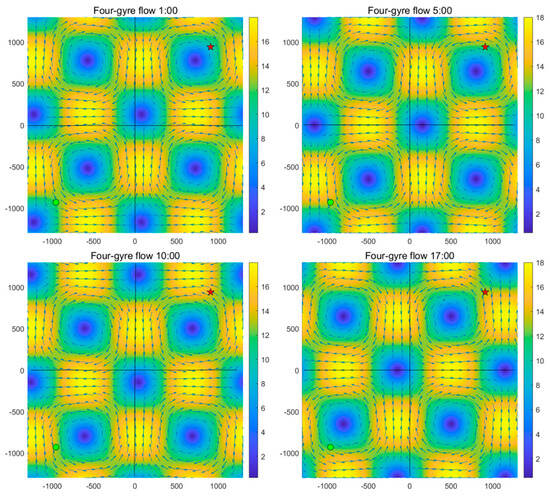
Figure 4.
Four time slices of four-vortex wind field changes within 24 h. The green dot represents the starting coordinates, and the red pentagram represents the ending coordinates.
To determine the optimal path in a dynamic four-vortex wind field, we employ GPOPS-II, a direct numerical optimization method based on the Gaussian pseudospectral method, as the benchmark. GPOPS-II utilizes the Legendre–Gauss–Radau pseudospectral discretization technique, transforming the optimal control problem into a finite-dimensional nonlinear programming (NLP) problem, which is globally optimized using the SNOPT solver [9]. This path is compared against the LS-PSO-base method, which employs a fine grid resolution of 20 km × 20 km, and the multiresolution grid LS-PSO (LS-PSO-MRG) method, to evaluate their path planning performance and computational efficiency in dynamic wind environments. Both LS-PSO-base and LS-PSO-MRG methods employed 100 particles and were executed for 200 iterations. The LS-PSO-MRG method employs a three-stage adaptive grid strategy, progressively refining the level-set evolution accuracy. Grid resolutions of 100 km × 100 km, 50 km × 50 km, and 20 km × 20 km were used in iterations 1–66, 67–133, and 134–200, respectively. Additionally, the parameters of the fitness function were set as , , and .
The experimental results in Figure 5 demonstrate that the LS-PSO-MRG method achieves the same fitness value as the LS-PSO-base method while improving computational efficiency by 52%. Additionally, the velocity profiles obtained through particle swarm optimization closely match the final path. Compared to GPOPS-II, the maximum lateral deviation of the computed path is nearly 30 km (0.2% of the total path length).
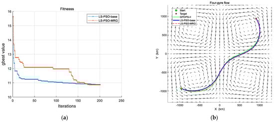
Figure 5.
Path planning results under four-gyre flow wind conditions. (a) Convergence comparison of the three-stage adaptive grid strategy and baseline LS-PSO over 200 Iterations. (b) Path optimization comparison: three-stage multi-resolution grid strategy LS-PSO (LS-PSO-MRG), baseline LS-PSO, and GPOPS-II. The black arrows indicate the wind field vectors at the initial moment.
As shown in Table 1, the total energy consumption achieved by both LS-PSO-Base and LS-PSO-MRG differs by less than 3% from that of GPOPS-II. This indicates that after 200 iterations, both LS-PSO-base and LS-PSO-MRG successfully converge near the optimal solution.

Table 1.
The performance of three path planning methods in the four-gyre wind field.
This experiment confirms the theoretical convergence of the LS-PSO algorithm in an ideal dynamic wind field and demonstrates that the multiresolution optimization strategy significantly reduces nearly half of the computation time while maintaining high-quality performance.
4.3. Cross-Day–Night Path Planning in ERA5 Reanalysis Wind Field
A realistic environment was constructed using ECMWF ERA5 reanalysis data [35], focusing on wind fields at the 70 hPa pressure (~18.5 km altitude) level for May and September 2024. The study area covers a 2000 km × 2000 km airspace centered on Dachaidan, Qinghai Province, China (37.85° N, 95.33° E), with a spatial resolution of 20 km × 20 km and a temporal resolution of 1 h. Two representative 24 h missions were selected to assess the algorithm’s performance under contrasting meteorological conditions, thereby demonstrating its adaptability across typical atmospheric regimes. All experiments in this section employed the enhanced LS-PSO algorithm with the multiresolution adaptive grid strategy, as described in Section 3.3.
In this case, we employed the LS-PSO algorithm to generate four distinct path types by adjusting the fitness function weights: energy-optimal arrival path with nighttime energy constraints (EC), time-optimal arrival path with nighttime energy constraints (TC), energy-optimal path without nighttime energy constraints (ENC), and energy–time-optimal path with nighttime energy constraints (ETC). All four paths utilized 100 particles and were executed over 200 iterations, employing the three-stage adaptive grid strategy with grid resolutions of 100 km × 100 km, 50 km × 50 km, and 20 km × 20 km for iterations 1–66, 67–133, and 134–200, respectively.
Additionally, the level-set path planning method (LSM) [24] was used to directly compute the time-optimal path under maximum-speed propulsion without nighttime energy constraints (TNC). LSM employs a fine grid for precise planning, with grid resolutions of 20 km × 20 km. The specific path types and their parameters are summarized in Table 2.
Table 2.
The parameters for different path strategies in this paper.
Case I: In A Dynamic Gyre Structure Flow
This case is designed to evaluate the adaptability of the proposed algorithm under rapidly changing wind conditions. Figure 6 illustrates the variations in wind speed and direction over the 24 h period from 13:00 on May 12 to 13:00 on May 13 2024 (UTC+8) in the target region. The wind direction is defined as 0 degrees when the wind vector points due north. It can be observed that both wind speed and direction fluctuate significantly over 24 h, including a six-hour period of sustained southerly winds (with an average wind vector angle exceeding 90°) from 23:00 on May 12 to 05:00 on May 13. As shown in Figure 7, the background wind field exhibits a clockwise gyre structure. The continuous displacement of the gyre center throughout the 24 h period results in substantial wind direction shifts.
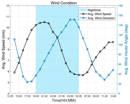
Figure 6.
Wind speed and wind vector angle between task start and target points in Dachaidan from 13:00 on 12 May to 13:00 on 13 May 2024.
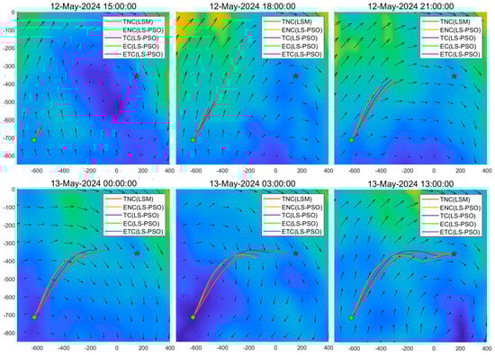
Figure 7.
Path planning results of different strategies at six time slices over a 24 h period in the dynamic gyre-structured flow.
The trajectories and corresponding propulsion speed profiles derived from different strategies are illustrated in Figure 6 and Figure 7. It is evident that the LSM, which neglects energy trade-offs, produces a TNC path characterized by a constant maximum airspeed directly toward the target. This trajectory is minimally affected by wind direction changes and results in the shortest path but significantly higher energy consumption during nighttime operations. In contrast, all other trajectories incorporate energy constraints or aim for energy-optimal performance, reflecting strategic compromises between wind exploitation and propulsion energy efficiency. The TC strategy prioritizes approaching the target before sunset, followed by a deliberate deviation from the shortest path during nighttime, reducing the airspeed from 12 m/s to approximately 8 m/s, and subsequently resuming high-speed flight after sunrise. The EC and ENC paths, which are nearly identical, closely follow wind streamlines to maximize wind-assisted energy savings. The ETC strategy represents a compromise between TC and EC, exhibiting a moderate trajectory that balances flight duration and energy consumption.
Analysis of the airspeed profiles in Figure 8 reveals a clear distinction between high-speed and energy-conserving cruising modes. The TNC strategy maintains a constant airspeed of 12 m/s throughout. The TC strategy exhibits a significant nighttime speed reduction to approximately 8 m/s, recovering to high speed after sunrise. In contrast, the energy-oriented strategies—ENC, EC, and ETC—maintain a steady airspeed between 7 and 8 m/s. Under prevailing southward winds between 23:00 and 05:00, the ETC and TC strategies allocate higher airspeeds than EC and ENC to mitigate adverse wind conditions and accelerate transit time.
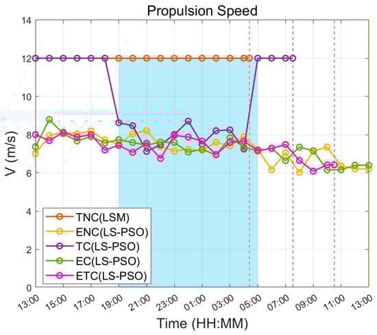
Figure 8.
Hourly propulsion speed profiles over a 24 h period under the dynamic gyre-structured flow for different strategies.
The quantitative results in Table 3 further validate these observations. The TC trajectory, through proactive daytime path adjustments, reduced the nighttime propulsion energy by 64.8% compared to TNC, achieving , significantly lower than TNC’s 37.63 kWh. The EC path demonstrated the most effective wind utilization, resulting in the lowest total energy consumption (24.91 kWh) despite being 32.67 km longer than the TNC path. The ETC strategy, with only a moderate increase in flight duration (21.38 h), achieved substantial reductions in both nighttime (11.43 kWh) and total energy consumption (30.22 kWh), thereby confirming the effectiveness of energy–time co-optimization for missions constrained by nighttime energy availability.
Table 3.
Path planning metrics in this case for different strategies.
We further analyzed the evolution of the reachable-set fronts generated by the LSM and LS-PSO schemes. Figure 9 depicts the evolution of reachable fronts by level-set forward propagation for the TNC, TC, and EC strategies prior to reaching the target, where the black contours represent daytime propagation and the blue contours represent nighttime propagation. The red crosses indicate the optimal trajectory points obtained from the target via level-set backward evolution. The three panels clearly expose how the objective and the nighttime energy constraint reshape flight reachability: in the TNC case, the vehicle cruises at a constant high speed, so the daytime and nighttime fronts expand almost concentrically. With the nighttime energy constraint, the TC solution still pushes the daytime front rapidly toward the goal, but its nighttime front markedly contracts and is stretched downstream by the prevailing wind into a teardrop form, indicating a strategy that saves energy by slowing down and drifting with the wind while preserving mission time. The EC solution, designed for minimum energy, exhibits the slowest expansion in both phases and the most elongated envelope, which consistently drifts along the wind direction, reflecting a low-speed, wind-assisted trajectory throughout the entire flight.
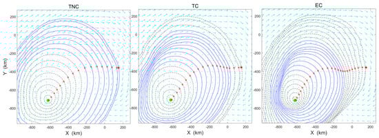
Figure 9.
Reachable set fronts and resulting path points over 24 h for TNC, TC, and EC strategies in Case I. The black contours represent daytime propagation and the blue contours represent nighttime propagation. The red crosses indicate the optimal trajectory points obtained from the target via level-set backward evolution.
The experimental results show the algorithm’s capability for path planning with complex energy–time-constraint tradeoffs in dynamic environments, providing actionable insights for mission planners balancing operational objectives with energy budgets.
Case II: In A Dynamic Headwind Flow
This section evaluates the algorithm’s adaptability under prolonged headwind conditions occurring throughout September. As shown in Figure 10, during the period from 13:00 on September 12 to 13:00 on September 13, the angle between the wind direction and the target direction consistently exceeded 90 degrees. Between 13:00 and 19:00, the wind formed the largest opposing angle with the target direction, which gradually decreased as nighttime approached.
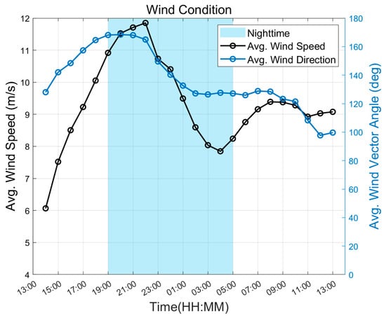
Figure 10.
Wind speed and wind vector angle between task start and target points from 13:00 on 12 September to 13:00 on 13 September 2024.
In Figure 11 and Figure 12, the EC path (green path) and the ENC path exhibit a spontaneous circling and waiting behavior—remaining near the starting position during the unfavorable daytime easterly winds (13:00–21:00) and leveraging the nighttime westerly winds for efficient propulsion. Compared to the TC path (purple), the EC path reduces energy consumption by 21.7% through strategic speed modulation, whereas the TC path prioritizes arrival time at the cost of a 28.6% increase in energy expenditure (see Table 4). Additionally, the TC path aggressively advances at maximum flight speed during the day and proactively reduces speed at night to comply with nighttime energy constraints. Computational efficiency remained robust, with LS-PSO-based path planning requiring 0.57–0.62 h, demonstrating practical feasibility for operational deployment.
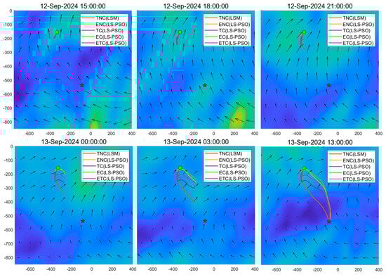
Figure 11.
Path planning results of different strategies at six time slices over a 24 h period in the dynamic headwind flow.
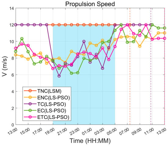
Figure 12.
Hourly propulsion speed profiles over a 24 h period under in the dynamic headwind flow for different strategies.
Table 4.
Path planning metrics under dynamic headwind flow influence for different strategies.
Figure 13 further visualizes how the optimization objective and nighttime energy constraints reshape the spatiotemporal reachability of different strategies under the LS-PSO framework. In the TNC plot, the reachable fronts expand broadly and symmetrically in both day and night due to a constant high propulsion speed without energy restrictions. In contrast, in the TC panel the daytime front still surges outward, yet the nighttime front is visibly pinched and stretched downstream, evidencing the deliberate slowdown and wind-drift adopted to respect the nighttime energy budget. Finally, in the EC panel the innermost blue contours clusters tightly around the start location that enables the vehicle to “wait out” the unfavorable winds; only after nightfall do the fronts elongate along the prevailing flow, following wind-aligned contours all the way to the goal.
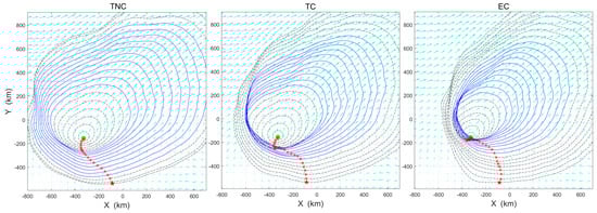
Figure 13.
Reachable set fronts and resulting path points over 24 h for TNC, TC and EC strategies in Case II. The black contours represent daytime propagation and the blue contours represent nighttime propagation. The red crosses indicate the optimal trajectory points obtained from the target via level-set backward evolution.
These results highlight the algorithm’s ability to synthesize context-aware path planning policies—whether prioritizing immediate progress (TC) or energy conservation (EC). The waiting behavior under severe headwinds provides empirical validation of the method’s capacity for non-myopic decision making, a critical requirement for long-duration stratospheric missions.
5. Discussion
The LS-PSO framework establishes a novel paradigm for stratospheric airship path planning by defining the integration mechanism between level-set methods and swarm intelligence algorithms. In this architecture, PSO searches the optimal velocity sequences while the level-set method evaluates them to determine their spatiotemporal reachability within dynamic flows. The resulting reachability data inform the PSO fitness evaluation for energy and time optimization. Finally, the optimal velocity sequence identified by the PSO undergoes backward level-set evolution to reconstruct trajectories that inherently satisfy both kinematic feasibility and energy constraints. This synergy allows the level-set component to rigorously verify path feasibility under time-varying conditions, while the PSO systematically explores constraint-satisfying velocity profiles—surpassing conventional fixed-speed level-set approaches in multi-objective adaptability. Synthetic four-gyre flow experiments quantitatively validate the framework’s precision, showing less than 3% deviation from pseudospectral optimization benchmarks, while the hierarchical grid adaptation strategy reduced computational costs by 52% without compromising solution quality, enabling full 24 h path planning to be completed 0.5 h. The reanalysis wind field path planning tests reveal the method’s capacity to generate a refined path that adaptively balances dynamic wind exploitation and energy conservation, with behaviors like spontaneous circling and waiting during adverse winds demonstrating improved environmental responsiveness over traditional methods.
While the LS-PSO framework demonstrates substantial improvements over conventional methods, its inherent limitations warrant careful consideration. First, the computational complexity escalates significantly for missions exceeding 24 h durations, as the combinatorial explosion of velocity sequence permutations challenges the PSO’s convergence efficiency. Second, the framework’s performance remains sensitive to wind prediction accuracy, particularly under evolving stratospheric weather patterns where forecast errors may compromise path optimality. Third, the simplified kinematic airship model (Equation (1)), which neglects transient aerodynamic effects and simplifies the vehicle as a point mass, may limit fidelity in scenarios requiring high maneuverability or precise attitude control—a necessary trade-off to maintain computational tractability in large-scale spatiotemporal planning. These constraints reflect broader challenges in autonomous path planning systems, balancing model fidelity with operational practicality. Future iterations could mitigate these limitations through probabilistic wind field assimilation, reduced-order reachability modeling, and enhanced dynamic models incorporating rotational kinematics, potentially improving robustness against meteorological uncertainties while expanding applicability to complex flight regimes.
The LS-PSO framework supports potential extensions beyond energy and time optimization. The level-set method allows it to naturally handle complex missions, such as station-keeping planning in specific areas. Future adaptations could integrate photovoltaic input models into the fitness function, enabling the joint optimization of propulsion energy consumption and solar charge potential. Additionally, the framework can easily incorporate obstacle avoidance capabilities in the forward evolution of the level set [29], eliminating the need for explicit penalty terms in constrained airspace scenarios. Beyond stratospheric airship applications, the core methodology offers insights for other autonomous systems operating in dynamic fluid environments, such as underwater vehicles navigating ocean currents or drones in urban wind fields. While the current study focuses on foundational validation, further improvements—like adaptive grid refinement or uncertainty-aware wind modeling—could broaden its practicality for diverse scenarios, paving the way for more robust energy-aware path planning systems in the future.
Author Contributions
Conceptualization, C.L. and X.L.; methodology, C.L.; software, C.L. and X.L.; validation, X.L., C.L., J.M. and Y.F.; formal analysis, C.L. and X.L.; investigation, Y.F.; resources, C.B.; data curation, Y.F.; writing—original draft preparation, X.L.; writing—review and editing, C.L.; visualization, X.L.; supervision, C.B. and C.L.; project administration, C.B. and C.L.; funding acquisition, C.B. and J.M. All authors have read and agreed to the published version of the manuscript.
Funding
This research and the APC was funded by the Pre-Research Project on Civil Aerospace Technologies grant number D030312.
Data Availability Statement
The data are contained within the article.
Conflicts of Interest
The authors declare no conflicts of interest.
References
- Parsa, A.; Monfared, S.B.; Kalhor, A. Backstepping Control based on Sliding Mode for Station-Keeping of Stratospheric Airship. In Proceedings of the 2018 6th RSI International Conference on Robotics and Mechatronics (IcRoM), Tehran, Iran, 23–25 October 2018; IEEE: Piscataway, NJ, USA, 2018; pp. 554–559. [Google Scholar] [CrossRef]
- Liao, L.; Pasternak, I. A review of airship structural research and development. Prog. Aerosp. Sci. 2009, 45, 83–96. [Google Scholar] [CrossRef]
- Hepp, A.F.; Kumta, P.N.; Velikokhatnyi, O.I.; Datta, M.K. Batteries for aeronautics and space exploration: Recent developments and future prospects. In Lithium-Sulfur Batteries; Elsevier: Amsterdam, The Netherlands, 2022; pp. 531–595. [Google Scholar] [CrossRef]
- Wu, J.; Fang, X.; Wang, Z.; Hou, Z.; Ma, Z.; Zhang, H.; Dai, Q.; Xu, Y. Thermal modeling of stratospheric airships. Prog. Aerosp. Sci. 2015, 75, 26–37. [Google Scholar] [CrossRef]
- Liu, S.; Zhou, S.; Miao, J.; Shang, H.; Cui, Y.; Lu, Y. Autonomous Trajectory Planning Method for Stratospheric Airship Regional Station-Keeping Based on Deep Reinforcement Learning. Aerospace 2024, 11, 753. [Google Scholar] [CrossRef]
- Shaw, J.A.; Nugent, P.W.; Kaufman, N.A.; Pust, N.J.; Mikes, D.; Knierim, C.; Faulconer, N.; Larimer, R.M.; DesJardins, A.C.; Knighton, W.B. Multispectral imaging systems on tethered balloons for optical remote sensing education and research. J. Appl. Remote Sens. 2012, 6, 063613. [Google Scholar] [CrossRef]
- Ning, X.; Liu, P.; Pan, Z. The Mechanical Characteristics and Experimental Study of the Stratospheric Airship. J. Appl. Math. Phys. 2021, 09, 183–196. [Google Scholar] [CrossRef]
- Ramesh, S.S.; Lim, K.M.; Lee, H.P.; Khoo, B.C. Reduced-Order Modeling of Stratospheric Winds and Its Application in High-Altitude Balloon Trajectory Simulations. J. Appl. Meteorol. Climatol. 2017, 56, 1753–1766. [Google Scholar] [CrossRef]
- Yang, X. Renewable power system simulation and endurance analysis for stratospheric airships. Renew. Energy 2017, 113, 1070–1076. [Google Scholar] [CrossRef]
- Song, K.; Li, Z.; Zhang, Y.; Wang, X.; Xu, G.; Zhang, H. A rule-based online energy management strategy for long-endurance stratospheric airships. Aerosp. Sci. Technol. 2024, 151, 109266. [Google Scholar] [CrossRef]
- Shan, C.; Lv, M.; Sun, K.; Gao, J. Analysis of energy system configuration and energy balance for stratospheric airship based on position energy storage strategy. Aerosp. Sci. Technol. 2020, 101, 105844. [Google Scholar] [CrossRef]
- D’Oliveira, F.A.; Melo, F.C.L.D.; Devezas, T.C. High-Altitude Platforms—Present Situation and Technology Trends. J. Aerosp. Technol. Manag. 2016, 8, 249–262. [Google Scholar] [CrossRef]
- Zhu, W.; Zhang, B.; Zhang, L.; Xu, Y.; Yang, K. Spatial path analysis for high-altitude solar-powered airship with maximum net energy. Aerosp. Sci. Technol. 2021, 117, 106922. [Google Scholar] [CrossRef]
- Zhang, L.; Li, J.; Jiang, Y.; Du, H.; Zhu, W.; Lv, M. Stratospheric airship endurance strategy analysis based on energy optimization. Aerosp. Sci. Technol. 2020, 100, 105794. [Google Scholar] [CrossRef]
- Xiao, L.; Zhou, P.; Wu, Y.; Lin, Q.; Jing, Y.; Yu, D. Trajectory planning with minimum energy consumption for multi-target regions autonomous cruise of stratospheric airship in wind field. Aerosp. Syst. 2023, 6, 521–529. [Google Scholar] [CrossRef]
- Zhang, Z.; Wan, Y.; Wang, Y.; Guan, X.; Ren, W.; Li, G. Improved hybrid A* path planning method for spherical mobile robot based on pendulum. Int. J. Adv. Robot. Syst. 2021, 18, 1729881421992958. [Google Scholar] [CrossRef]
- Zhang, Y.; Yang, K.; Chen, T.; Zheng, Z.; Zhu, M. Integration of path planning and following control for the stratospheric airship with forecasted wind field data. ISA Trans. 2023, 143, 115–130. [Google Scholar] [CrossRef]
- Luo, Q.; Sun, K.; Chen, T.; Zhang, Y.; Zheng, Z. Trajectory planning of stratospheric airship for station-keeping mission based on improved rapidly exploring random tree. Adv. Space Res. 2024, 73, 992–1005. [Google Scholar] [CrossRef]
- Wang, J.; Chi, W.; Li, C.; Wang, C.; Meng, M.Q.-H. Neural RRT*: Learning-Based Optimal Path Planning. IEEE Trans. Autom. Sci. Eng. 2020, 17, 1748–1758. [Google Scholar] [CrossRef]
- Mitra, A.; Talukder, A.; Willets, J.; Atajanova, L.; Ganesh, R.; Sha, W. Enhancing Cargo Transportation by Reducing Airship Operating Costs; 2024. Available online: https://ntrs.nasa.gov/api/citations/20240012628/downloads/NASA-TM-20240012628.pdf (accessed on 17 March 2025).
- Hou, J.; Zhu, M.; Zheng, B.; Guo, X.; Ou, J. Trajectory Planning Based On Continuous Decision Deep Reinforcement Learning for Stratospheric Airship. In Proceedings of the 2023 China Automation Congress (CAC), Chongqing, China, 17–19 November 2023; IEEE: Piscataway, NJ, USA, 2023; pp. 1508–1513. [Google Scholar] [CrossRef]
- Hu, S.; Wang, B.; Zhang, A.; Deng, Y. Genetic Algorithm and Greedy Strategy-Based Multi-Mission-Point Route Planning for Heavy-Duty Semi-Rigid Airship. Sensors 2022, 22, 4954. [Google Scholar] [CrossRef]
- Zeng, Z.; Sammut, K.; Lian, L.; He, F.; Lammas, A.; Tang, Y. A comparison of optimization techniques for AUV path planning in environments with ocean currents. Robot. Auton. Syst. 2016, 82, 61–72. [Google Scholar] [CrossRef]
- Lolla, T.; Ueckermann, M.P.; Yigit, K.; Haley, P.J.; Lermusiaux, P.F.J. Path planning in time dependent flow fields using level set methods. In Proceedings of the 2012 IEEE International Conference on Robotics and Automation, St Paul, MN, USA, 14–18 May 2012; IEEE: Piscataway, NJ, USA, 2012; pp. 166–173. [Google Scholar]
- Lolla, T.; Haley, P.J.; Lermusiaux, P.F.J. Time-optimal path planning in dynamic flows using level set equations: Realistic applications. Ocean Dyn. 2014, 64, 1399–1417. [Google Scholar] [CrossRef]
- Chen, H.; Ma, Y.; Hu, W.; Cao, C. Time and Risk Optimal Path Planning for Surface Vehicle via Level Set in Dynamic Environment. IEEE Trans. Ind. Inform. 2024, 20, 8639–8649. [Google Scholar] [CrossRef]
- Qin, H.; Shao, S.; Wang, T.; Yu, X.; Jiang, Y.; Cao, Z. Review of Autonomous Path Planning Algorithms for Mobile Robots. Drones 2023, 7, 211. [Google Scholar] [CrossRef]
- Li, D.; Wang, P.; Du, L. Path Planning Technologies for Autonomous Underwater Vehicles-A Review. IEEE Access 2019, 7, 9745–9768. [Google Scholar] [CrossRef]
- Zhu, J.; Shen, H.; Tang, Q.; Qin, Z.; Yu, Y. Energy-Efficient Route Planning Method for Ships Based on Level Set. Sensors 2025, 25, 381. [Google Scholar] [CrossRef]
- Tang, J.; Xie, W.; Zhou, P.; Yang, H.; Zhang, T.; Wang, Q. Multidisciplinary Optimization and Analysis of Stratospheric Airships Powered by Solar Arrays. Aerospace 2023, 10, 43. [Google Scholar] [CrossRef]
- Yang, X.; Liu, D. Conceptual Design of Stratospheric Airships Focusing on Energy Balance. J. Aerosp. Eng. 2018, 31, 04017094. [Google Scholar] [CrossRef]
- Mitchell, I.M. The Flexible, Extensible and Efficient Toolbox of Level Set Methods. J. Sci. Comput. 2008, 35, 300–329. [Google Scholar] [CrossRef]
- Mitchell, I.M.; Templeton, J.A. A Toolbox of Hamilton-Jacobi Solvers for Analysis of Nondeterministic Continuous and Hybrid Systems. In Hybrid Systems: Computation and Control; Morari, M., Thiele, L., Eds.; Lecture Notes in Computer Science; Springer: Berlin/Heidelberg, Germany, 2005; Volume 3414, pp. 480–494. [Google Scholar] [CrossRef]
- Patterson, M.A.; Rao, A.V. GPOPS-II: A MATLAB Software for Solving Multiple-Phase Optimal Control Problems Using hp-Adaptive Gaussian Quadrature Collocation Methods and Sparse Nonlinear Programming. ACM Trans. Math. Softw. 2014, 41, 1–37. [Google Scholar] [CrossRef]
- Hersbach, H.; Bell, B.; Berrisford, P.; Hirahara, S.; Horányi, A.; Muñoz-Sabater, J.; Nicolas, J.; Peubey, C.; Radu, R.; Schepers, D.; et al. The ERA5 global reanalysis. Q. J. R. Meteorol. Soc. 2020, 146, 1999–2049. [Google Scholar] [CrossRef]
- Schnitzler, B.; Drouin, A.; Moschetta, J.-M.; Delahaye, D. General Extremal Field Method for Time-Optimal Trajectory Planning in Flow Fields. IEEE Control Syst. Lett. 2023, 7, 2605–2610. [Google Scholar] [CrossRef]
- Kularatne, D.; Bhattacharya, S.; Ani Hsieh, M. Time and Energy Optimal Path Planning in General Flows. In Robotics: Science and Systems XII; Robotics: Science and Systems Foundation: Los Altos, CA, USA, 2016. [Google Scholar] [CrossRef]
- Greatbatch, R.J.; Nadiga, B.T. Four-Gyre Circulation in a Barotropic Model with Double-Gyre Wind Forcing. J. Phys. Oceanogr. 2000, 30, 1461–1471. [Google Scholar] [CrossRef]
Disclaimer/Publisher’s Note: The statements, opinions and data contained in all publications are solely those of the individual author(s) and contributor(s) and not of MDPI and/or the editor(s). MDPI and/or the editor(s) disclaim responsibility for any injury to people or property resulting from any ideas, methods, instructions or products referred to in the content. |
© 2025 by the authors. Licensee MDPI, Basel, Switzerland. This article is an open access article distributed under the terms and conditions of the Creative Commons Attribution (CC BY) license (https://creativecommons.org/licenses/by/4.0/).