Article

Deep Learning Framework for Predicting Transonic Wing Buffet Loads Due to Structural Eigenmode-Based Deformations

Chair of Aerodynamics and Fluid Mechanics, Technical University of Munich, 85748 Garching bei München, Germany
*
Author to whom correspondence should be addressed.
Aerospace 2025, 12(5), 415; https://doi.org/10.3390/aerospace12050415
Submission received: 14 April 2025 / Revised: 30 April 2025 / Accepted: 6 May 2025 / Published: 7 May 2025
(This article belongs to the Section Aeronautics)

Abstract

:
In the present paper, a reduced-order modeling (ROM) approach based on a hybrid neural network is presented in order to calculate wing buffet pressure distributions due to structural eigenmode-based deformations. The accurate prediction of unsteady surface pressure distributions is crucial for assessing aeroelastic stability and preventing structural failure, but full-order simulations are computationally expensive; the proposed ROM provides a fast and efficient alternative with a sufficient level of accuracy. The hybrid ROM is defined by a series connection of a convolutional autoencoder (CNN-AE) and a long short-term memory (LSTM) neural network. As a test case, the NASA Common Research Model (CRM) configuration for the transonic buffet condition is applied. Forced-motion computational fluid dynamics (CFD) simulations are conducted in order to obtain the aerodynamic responses induced by the eigenmode-based deformations. For the unsteady simulations, the triangular adaptive upwind (TAU) solver of the German Aerospace Center (DLR), is used. Based on a selected structural model, symmetric and asymmetric eigenmode-based deformations of the wing structure are implemented and considered for performance evaluation. Comparing the pressure loads modeled by the hybrid ROM and the reference full-order numerical solution, an overall good prediction performance is indicated with mean squared error (MSE) values mostly below 3 % , reaching local maxima of about 12 % , due to strong pressure gradients associated with pronounced shock oscillations.

1. Introduction

Transonic buffet, which is also commonly referred to as wing shock buffet, is defined as a self-sustained pre-stall instability, characterized by shock-wave oscillations in the chord- and spanwise directions and intermittent boundary layer separation. Due to the detached flow on the wing suction side, the wing structure is excited, which is called buffeting. Due to buffeting, passenger comfort during flight is drastically reduced and the wing structure is susceptible to material fatigue. Therefore, a precise determination of structural loads due to buffeting is of paramount importance for the safety of any civil aircraft.
Nowadays, high-fidelity computational fluid dynamics (CFD) methods such as unsteady Reynolds-averaged Navier Stokes (URANS) or Detached-Eddy Simulation (DES) are applied to a large extent for the investigation of three-dimensional buffet [1,2]. Further, experiments with half- and full-span wind tunnel models have been conducted for the determination of buffet loads [3,4]. However, although high-performance computers and experimental facilities are available, the accurate computation of the loads due to buffet and buffeting is still challenging due to the high computational costs and time, especially if applied in an industrial context.
Besides the application of high-fidelity solutions, system identification methods for unsteady aerodynamic modeling gained increasing attention in recent years. These methods are able to represent an aerodynamic system with a reduced number of degrees of freedom compared to the original system. Therefore, they are referred to as reduced-order models (ROMs). Considering an unsteady aerodynamic system, the inputs of the ROM are commonly defined by the motion of the body or the structural part of interest, whereas the output represents the resulting integral and local aerodynamic characteristics [5].
Focusing on the application of ROM methods for unsteady aerodynamic modeling, Wiener models [6], Volterra series [7] and Kriging models [8] can be mentioned as some of the first successful approaches. Besides these ROMs, standard recurrent neural networks (RNNs) [9] and radial basis function neural networks (RBFNNs) [10,11] have been used for the prediction of limit cycle oscillations and airfoil load prediction. Further, in Reference [12], a nonlinear hybrid ROM based on a recurrent neuro-fuzzy model (NFM) and a multilayer perceptron (MLP) neural network was proposed. Reference [13] deals with the application of a long short-term memory (LSTM) neural network for the prediction of integral buffet characteristics due to forced-motion excitation.
Focusing on the prediction of spatial characteristics such as wing pressure distributions, the nonlinear ROMs mentioned above are not applicable due to the size of the resulting output and the large computational time. Therefore, dimensionality reduction techniques such as Proper Orthogonal Decomposition (POD) and Dynamic Mode Decomposition (DMD) have been applied in several studies. Considering buffet aerodynamics, Timme [14] and Ohmichi et al. [15] used POD and DMD in order to extract important modes of the buffet instability and characterize the flow physics. A study by Chandon et al. [16] applied DMD for the prediction of bending and torsion loads due to buffet on a high-agility aircraft.
In addition to the application of POD and DMD, convolutional neural networks (CNNs) and autoencoder structures are applicable for the computation of the spatial characteristics of high-dimensional flow field data and data reduction, respectively. Studies by Afshar et al. [17] and Sekar et al. [18] applied a CNN-based ROM for the computation of the flow and pressure field around an airfoil in transonic flow. Besides the application of a single CNN structure, recent studies proposed hybrid deep learning models based on CNNs and recurrent neural networks (RNNs). Li et al. [19] used a convolutional long short-term memory (ConvLSTM) neural network for flow field prediction through cascade channels. Hasegawa et al. [20] proposed a hybrid ROM based on a series connection of a convolutional autoencoder (CNN-AE) and a LSTM for unsteady flow field prediction. The proposed method was also used by Nakamura et al. [21] for turbulent channel flow prediction. Liu et al. [22] used a hybrid CNN-ConvLSTM for buffet flow field computation around an airfoil.
In the present study, the focus is on the application of a hybrid CNN-AE/LSTM based ROM for the prediction of buffet loads due to structural eigenmode-based deformations. Introducing a fundamentally new hybrid reduced-order modeling approach that couples a convolutional autoencoder with a LSTM network, for the first time, the rapid and highly accurate prediction of nonlinear buffet pressure distributions resulting from structural eigenmode deformations is shown. The structural deformations are imposed during an already developed buffet instability, resulting in a highly nonlinear flow field expected in the buffeting condition. As a test case, the NASA Common Research Model (CRM) is applied. The training, validation and test data sets are computed using the triangular adaptive upwind (TAU) flow solver developed by the German Aerospace Center (DLR). For structural modeling, the FERMAT structure model proposed by Klimmek [23] is applied. The deformations of the structure are implemented in the numerical solver using a Python interface. For the training of the hybrid ROM, forced-motion CFD simulations are conducted in order to obtain the wing buffet loads due to the induced structural deformations. Therefore, both symmetric and asymmetric deflections are implemented and simulated.

2. Deep Learning Approaches

Within the following section, the applied deep learning model is presented. The first part of the section includes a brief overview of the working principle of CNNs. In the second part, the LSTM neural network is introduced. The section is concluded with a description of the architecture of the applied hybrid neural network. All models are implemented in Python 3.11.3 using the PyTorch 2.0.1 library.

2.1. Convolutional Neural Network (CNN)

A convolutional neural network (CNN) is a type of neural network mainly designed for processing data characterized by a grid-like topology [24]. Although CNNs are to some extent applicable to time series and sequence data, they are commonly applied for the prediction of spatial information in data. The structure of a CNN is defined by three main layers: a convolutional layer, a pooling layer and a fully connected (FC) layer. Depending on the application scenario, several convolutional and pooling layers can be included in the overall architecture.
Assuming a data set defined as a three-dimensional matrix containing spatial information, the position of each data point can be defined by an index (i,j,o). Following the nomenclature of Goodfellow et al. [24] and Rosov and Breitsamter [25], the convolution can be defined as follows:
y i , j , o = l = 0 C i n 1 m = 0 H k 1 n = 0 W k 1 x l , i × s + m , j × s + n W o , l , m , n + b k
with x i , j , o denoting the input at index (i,j,o) of the input x . The size of the input is defined by its height H x and width W x as well as the number of input channels C i n ( C i n × H x × W x ). W represents a matrix containing the weights of the filter, which selects important features of the input data. Commonly, the filter is also referred to as the kernel and its size is defined by C i n × H k × W k × C o u t . Here, an additional dimension referred to as output channel C o u t is included, which represents the number of outputs arranged along the channel dimension [25].
The kernel slides stepwise over the input data, performing element-wise multiplications with the elements of the input matrix. Therefore, at each step, the filtered results are written as a new output. Besides the filtering operation, a technique defined as striding is applicable in order to reduce the dimension of the data. Choosing a stride s (see Equation (1)) equal to one, data points are picked an entry apart, resulting in the same output size as the input size. Selecting s = 2, the input size is reduced by a factor of two.
For this study, the structure of a CNN is used as an autoencoder architecture, which is referred to as a convolutional autoencoder (CNN-AE). A CNN-AE is trained in an unsupervised way using backpropagation (BP) [26], learning to encode a given input and reconstructing it to its output [24]. A common AE architecture is defined by an encoder, decoder and latent space, also referred to as a bottleneck. The task of the encoder is the reduction of high-dimensional data into the low-dimensional latent space, whereas the decoder extends the reduced data into its original dimension without losing any information related to the input data.

2.2. Long Short-Term Memory (LSTM) Neural Network

The LSTM neural network, as proposed by Hochreiter and Schmidhuber [27], represents a type of a RNN, which is able to predict both long- and short-term dependencies in data that involve sequences. Further, the application of a LSTM avoids a problem known as vanishing gradient [28], where the training performance saturates in the early stages of the training process.
Due to its characteristic gate structure, as depicted in Figure 1, the representation of time-delayed effects, which occur in unsteady aerodynamic systems, are already captured by the LSTM.
In contrast to a RNN, the hidden layer of a LSTM consists of recurrently connected blocks, which are referred to as memory blocks or cells. Each cell is defined by a gate structure, which processes the incoming information in several steps. The three gates, as shown in Figure 1, are defined as the forget gate f , the input gate i and the output gate o .
In the forget gate f , the input of the current time step x t and the vector representing the output from the previous time step h t 1 are combined and processed:
f t = σ ( W f x t + W f h t 1 + b f )
The output from the previous time step h t 1 is also referred to as the hidden state of the LSTM cell. Both inputs of the forget gate are multiplied with a set of weights W f and a bias b f is added. By applying a sigmoid ( σ ) activation, parts of the incoming information are discarded from the cell.
Equal to the forget gate f , the current time step x t and the hidden state from the previous time step h t 1 are combined and processed in the input gate i :
i t = σ ( W i x t + W i h t 1 + b i )
with W i and b i defining the weights and bias of the input gate, respectively. Further, a σ activation is applied.
In the second step, both inputs are processed by a hyperbolic tangent (tanh) activation, which creates a new cell state vector c ˜ t :
c ˜ t = t a n h ( W h x t + W h h t 1 + b h )
Based on the new cell state c ˜ t , the current cell state is updated with new information. Therefore, the cell state from the previous time step c t 1 is multiplied with the forget gate vector f t and the current cell state is updated with the input gate vector i t :
c t = f t c t 1 + i t c ˜ t
After passing the input gate, the data of the current input x t , the previous hidden state h t 1 and the current cell state c t are processed by a sigmoid and tanh activation:
o t = σ ( W o x t + W o h t 1 + b o ) h t = o t · t a n h ( c t )
The predictions, which are defined by the updated hidden state h t , are transferred to the next hidden layer or the output layer.
Based on the available numerical data set, the weights and biases are updated by applying backpropagation through time (BPTT) [29]. Therefore, the adaptive moment estimation (ADAM) [30] algorithm is applied.

2.3. Architecture of the Hybrid ROM

In order to enable an accurate and efficient representation of the forced-motion wing buffet pressure loads, the CNN-AE and the LSTM as introduced in Section 2.1 and Section 2.2 are connected into a hybrid ROM architecture. In Figure 2, the architecture of the hybrid ROM is visualized.
Both the encoder and the decoder of the CNN-AE are divided into several convolution and de-convolution levels. At each level, a number of operations are performed on the input data, which is processed by the encoder. The latent vector, which is defined by encoding the input data, is subsequently used as the input data for the LSTM. The model receives a sequence of numerically computed c p values of the wing suction side, which is defined by a tensor of N i n × C i n × H × W . Here, N i n is defined as the number of input time steps, C i n denotes the number of input channels, and H and W represent the number of grid points in the span- and chordwise directions, which are defined by powers of two in the present study.
At each level of the encoder, a multi-channel convolution with a kernel size of 4 × 4 , stride s = 2 and padding of one is applied. After passing the convolution layer, the input data are normalized using batch normalization (BN) [31]. Subsequently, a rectified linear unit (ReLU) activation is applied to each element of the input data. Due to the sequence of operations described above, the output channel size at each level is defined as two times the input channel size. In contrast, the size of the spatial dimensions ( H , W ) is reduced by a factor of two at each level of the encoder. After passing the different encoder levels, a ReLU activation is applied to the data. In the last steps, the data are flattened and passed through a FC and a tanh activation layer.
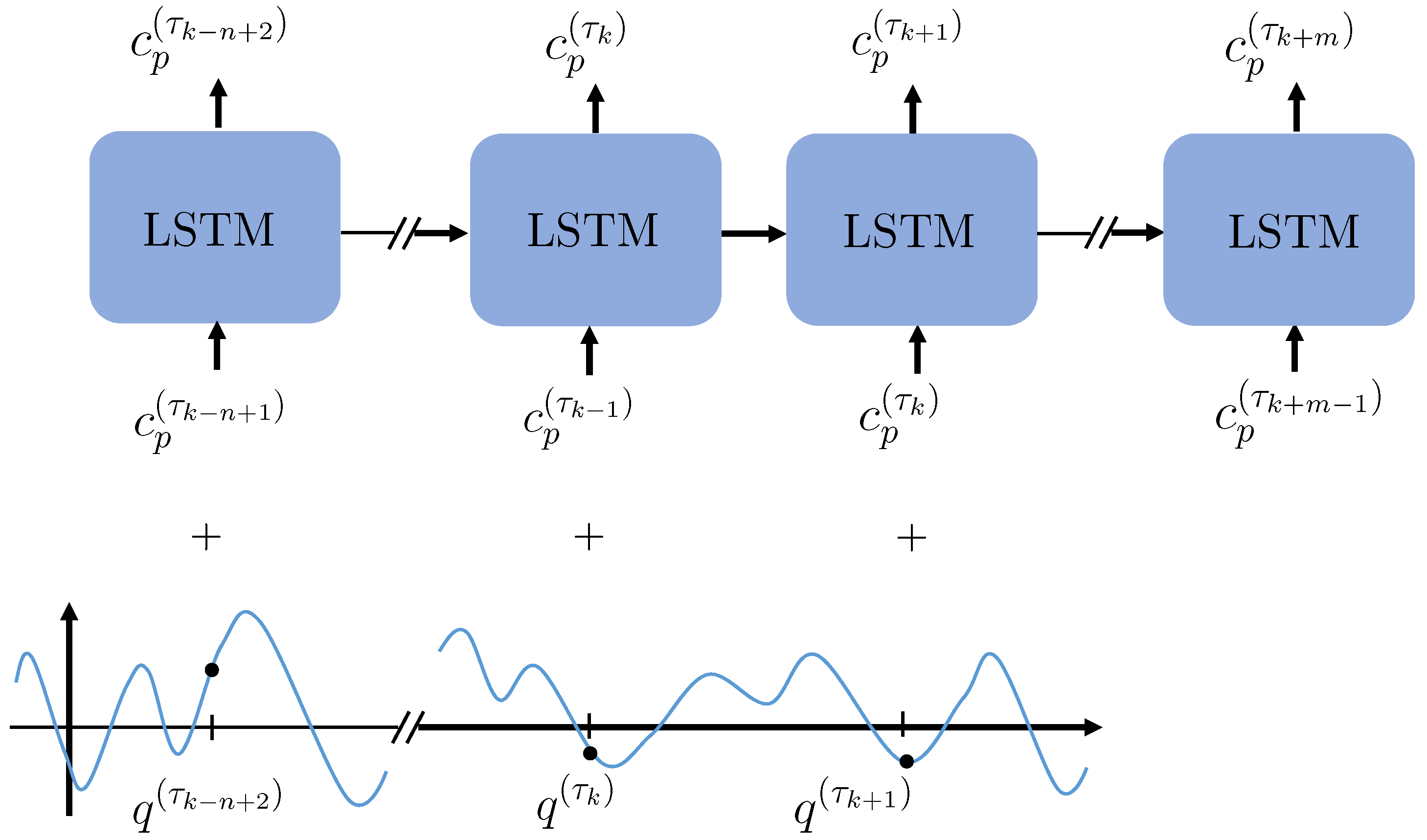
Before passing the encoded data into the LSTM, the information concerning the deformation Δ q and the c p data are combined. The aim is the prediction of pressure distributions at time steps k + m based on several previous c p -snapshots at time steps k n + 1 to k. Concerning the deformation, incidence amplitudes at time steps k n + 2 to k + 1 are considered. The scalar deformation values are concatenated to the end of the vector containing the c p values, as shown in Figure 3. The resulting latent vectors including both the c p -distribution and the deformation information are passed sequentially into the LSTM.
After passing the LSTM, the predicted data are fed into the decoder. At each level of the decoder, a transposed convolution is applied to upscale the spatial dimension. The corresponding kernel, stride and padding are chosen to equal those of the encoder. Further, BN is applied at each decoder level. At the final level, the decoded data are activated by a tanh layer, rescaling the value range of the data to [−1,1].

3. Test Case: NASA Common Research Model (CRM)

As a test case for the following investigations, the NASA CRM is applied. The configuration investigated in the present study represents a wing/body model with a horizontal tail plane. The design cruise condition is defined by a Mach number of M a = 0.85 and a lift coefficient of C L = 0.5 . For the following studies, both half- and full-span models of the CRM configuration are simulated for the buffet condition. In Figure 4, the geometry of the full-span model is visualized using isometric, top, front and back views.

3.1. Computational Setup

The hybrid computational grid employed in the present study has been generated and already applied in a numerical study by Ehrle et al. [32]. The simulation setup aims to replicate the conditions of a test campaign in the European Transonic Windtunnel (ETW) [33]. Based on the scale of the wind tunnel model, the geometric parameters summarized in Table 1 apply for the CRM configuration:
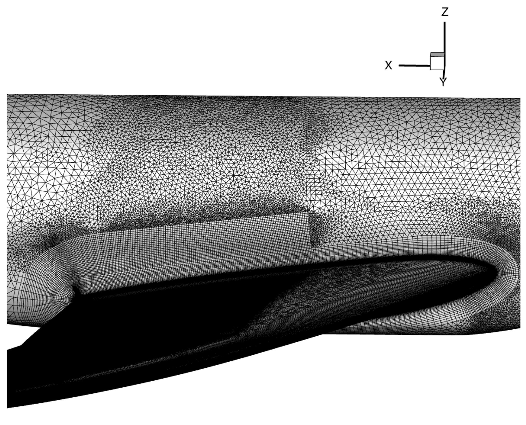
The grid of the half-span model is composed of approximately 36 × 10 6 elements, whereas the full-span model includes around 70 × 10 6 elements. Both grids are composed of unstructured cells in the farfield and structured cells around all surfaces with a proper boundary layer resolution with a minimum wall distance of the first cell of y + < 1. In addition, a refinement block containing uniform hexahedral elements is defined above the boundary layer elements on the wing’s suction side, in order to ensure a sufficient spatial resolution of the area of shock motion and flow separation (see Figure 5). The cell size of the block is defined according to a CFL (Courant–Friedrichs–Levy) number of 1.
The buffet condition of the applied CRM configuration is defined by a freestream Mach number of M a = 0.85, a Reynolds number of R e = 30 × 10 6 and an angle of attack of α = 5 . Aeroelastic wing deformations as encountered during a wind tunnel test campaign [33] are incorporated in the numerical grid by applying a static mesh deformation prior to the simulations. In order to approximate the buffet conditions in the wind tunnel, nitrogen is chosen as the working fluid.
For the generation of the training, validation and test data sets, URANS simulations for the computation of buffet related flow fields are conducted. The spatial discretization is accomplished by a central differencing scheme. In order to reduce the numerical dissipation of small-scale structures, a ratio of 0.4 between matrix and scalar dissipation in combination with a fourth-order dissipation coefficient of 1/256 was chosen. A Kok skew symmetric scheme is applied for the discretization of the meanflow fluxes, whereas the discretization of the turbulence fluxes is accomplished by a first order Roe scheme. A Green Gauss scheme is applied for the reconstruction of the gradients. Time integration is achieved using an implicit backward Euler scheme, whereas a LU-SGS scheme is chosen as a linear solver. Further, a 3 v multigrid cycle is applied to the grid in order to accelerate convergence. A dual time stepping approach is applied for all simulations with a physical time step of 1 × 10 5 s and 100 inner iterations per time step. Further, a CFL number of the implicit pseudo time steps of two is chosen. For turbulence modeling, the Spalart–Allmaras (SA) model without trip-term f t and turbulence suppression term f t 2 is employed. In addition, a quadratic constitutive relation (QCR) [34] extension is activated for the SA model. As shown by Togiti et al. [35], the combination of an eddy-viscosity turbulence model and the QCR leads to a reduced corner flow separation, which was observed by a numerical study at flight Reynolds numbers of the CRM by Illi et al. [36].

3.2. Validation of Computational Setup

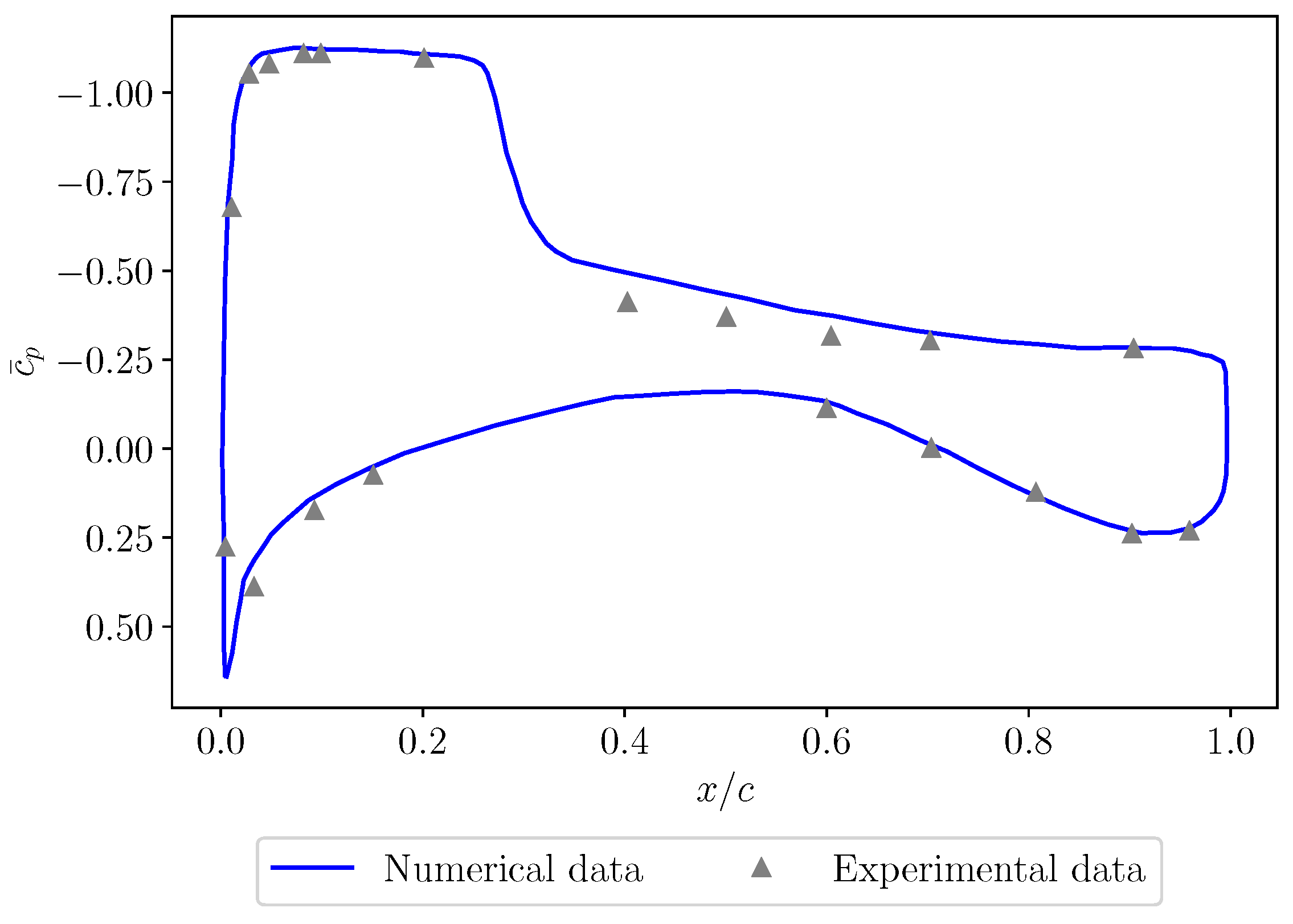
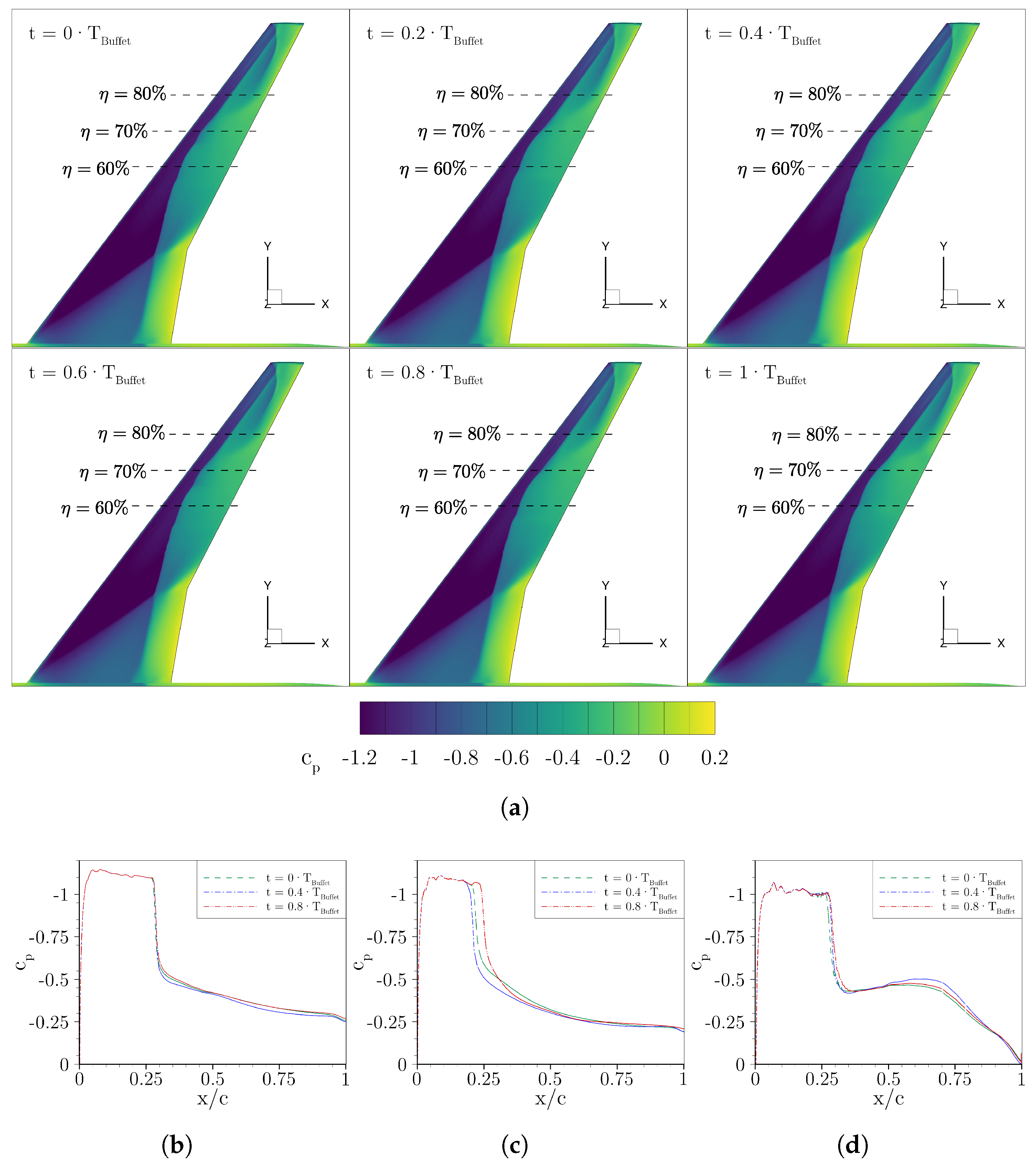
Applying the URANS setup described above, a buffet instability develops on the wing suction side. A comparison of the mean pressure coefficient c ¯ p [32] obtained by URANS with experimental data [33] showed a good agreement, with only minor deviations in the shock region. In Figure 6, a comparison of the experimental c ¯ p and the URANS solution at a spanwise position of η = 60% is visualized. In Figure 7, a series of six c p -snapshots representing a buffet period T B u f f e t , which is defined by 0.00665 s, is depicted. As shown, a characteristic λ -shaped two-shock pattern develops on the wing surface. Further, changes in the local surface pressure are shown for three distinct sections located at the spanwise positions of η = 60 % , 70 % and 80 % . Consistent with previous numerical studies [2], this indicates the convection of so-called buffet cells.

3.3. Implementation of Eigenmode-Based Deformations

For modeling the eigenmode-based structural deformations, the FERMAT configuration proposed by Klimmek [23] is applied. The finite element model (FEM) was developed in order to allow static and dynamic aeroelastic investigations on the basis of the CRM geometry, referring to a full-scale aircraft. The FERMAT model allows for the representation of two different setups, namely the C1 case representing the maximum zero fuel weight configuration and the C2 case, defining the configuration with maximum take-off weight. For the following investigation, the C2 mass configuration is applied. The C2 configuration includes in total 56 modes, representing six rigid body and 50 elastic modes.
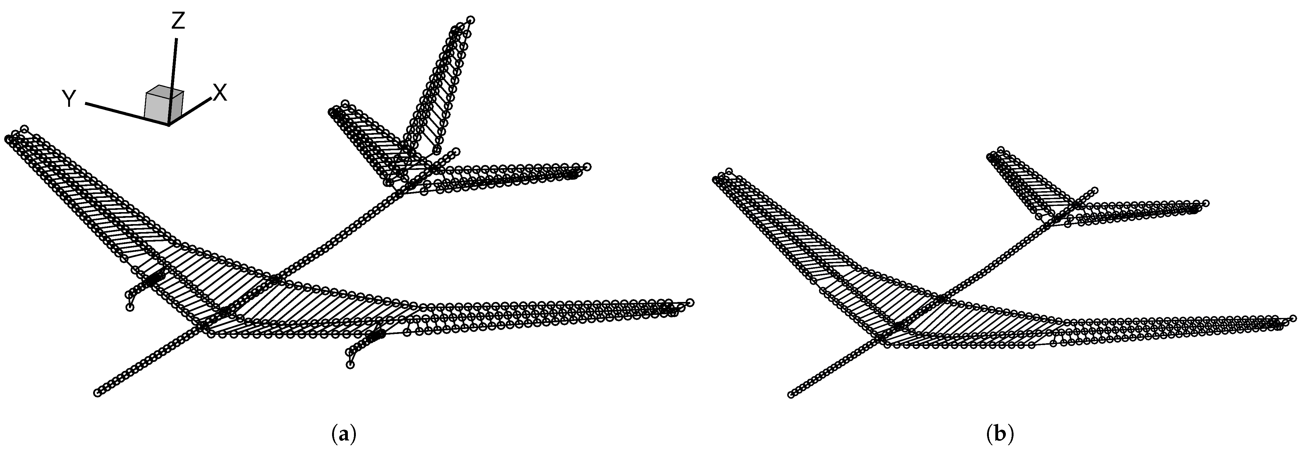
The FEM of the FERMAT configuration includes nodes for fuselage, wing, vertical (VTP) and horizontal (HTP) tail planes as well as pylons and engines. Since the numerical grid of the CRM only includes the fuselage, wing and HTP, the FEM is reduced for the surface interpolation between the structural and the aerodynamic surface grid. In Figure 8, a comparison of the original (left) and reduced (right) FEM is depicted.
The interpolation of the structural deflections on the surface grid is achieved using the thin-plate spline (TPS) algorithm. Since the focus of the investigation is on the wing buffet instability, only symmetric and asymmetric modes of the wing are considered in the present study.
Following the work of Refs. [37,38], the mode deflections are scaled proportionally with respect to the reference chord length c r e f . The resulting scaling factor S F is defined as follows:
S F = f · c r e f A m a x
with A m a x defining the maximum deflection amplitude of the considered mode and f denoting the reference scaling factor, which is chosen as f = 0.01 (1%). The factor is chosen in order to guarantee stable numerical simulations. In Figure 9, the considered mode shapes are visualized in comparison to the original CRM geometry. Here, an increased deflection is shown for clarity.

3.4. CFD-Based Data Set Generation

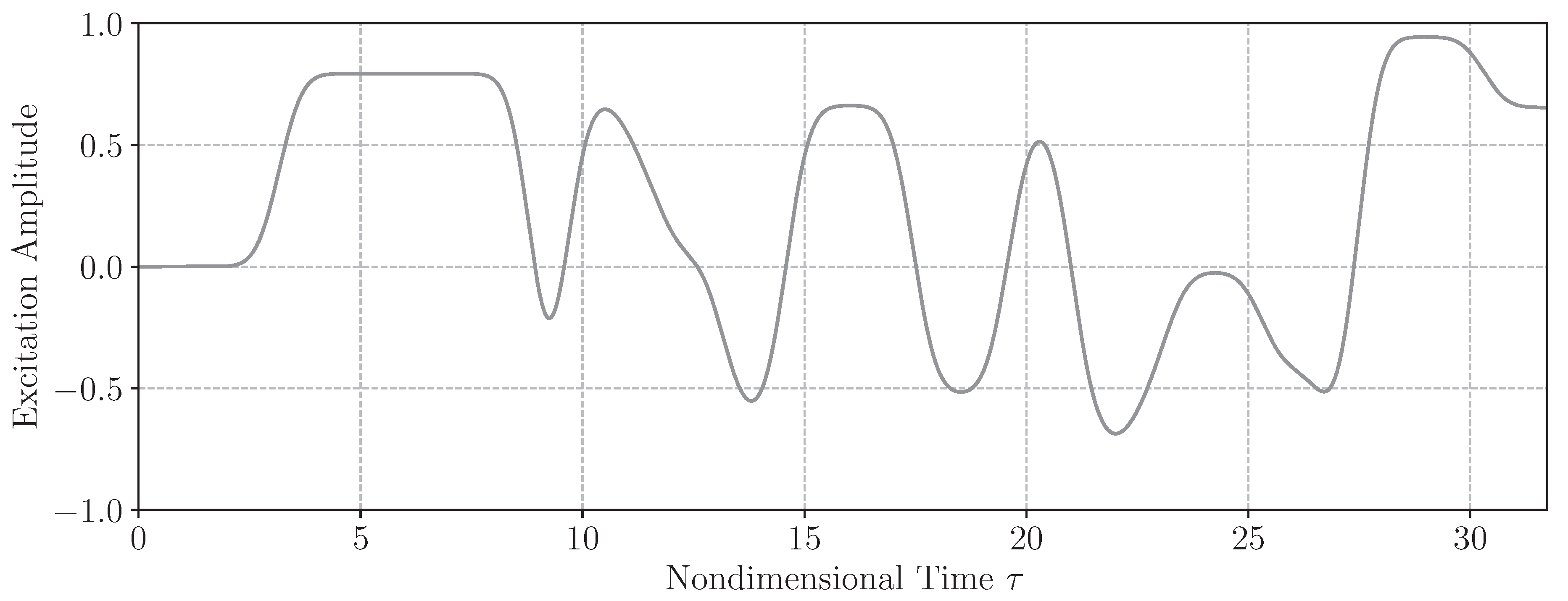
For the generation of the training and validation data sets, forced-motion CFD simulations are performed. For the time-based excitation of the mode shapes, a smoothed amplitude-modulated pseudo-random binary signal (SAPRBS) [39] is generated and applied. This signal type is used, since it is characterized by a high frequency and amplitude content, making it suitable for time and cost consuming simulations. The generated signal is depicted in Figure 10, including 2000 time steps.
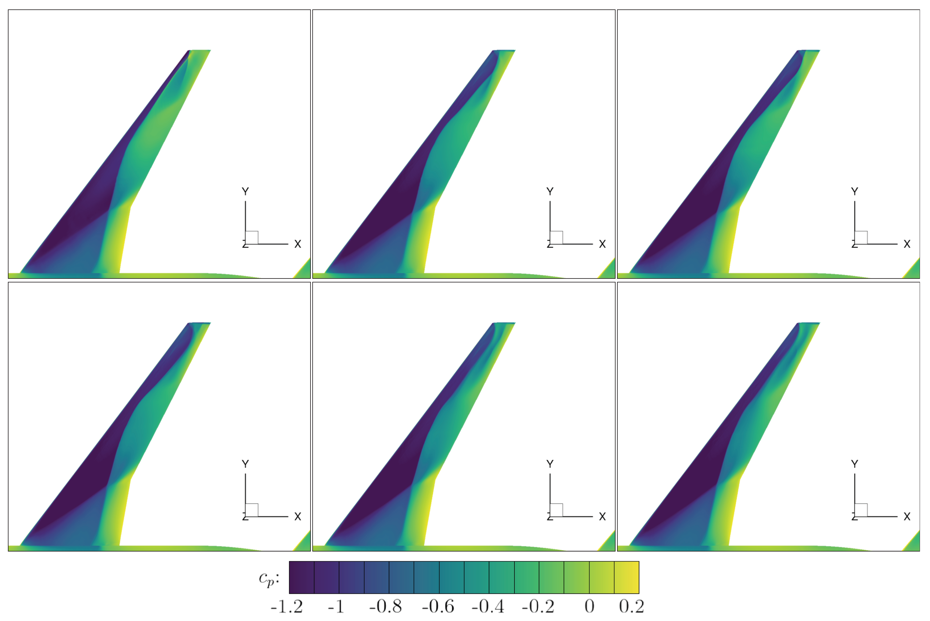
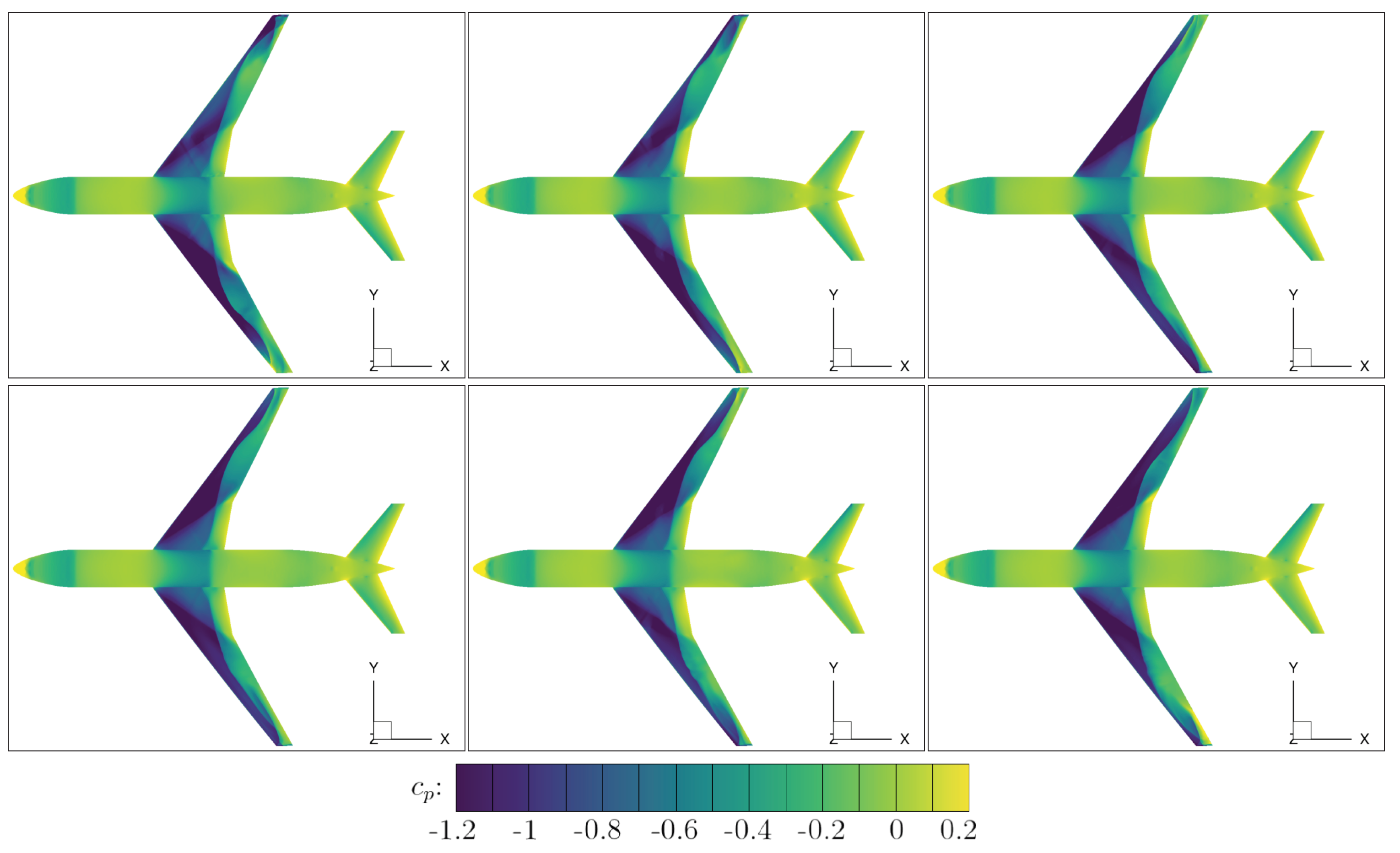
For all simulations, the minimum and maximum excitation amplitude of the signal are chosen to equal a reference scaling factor of f = 1%. Due to the excitation and the resulting structural deflection, clear changes in the surface c p on the wing suction side result. In Figure 11 and Figure 12, six consecutive c p -snapshots are visualized for the SAPRBS excitation of mode shapes 11 and 14, respectively.

4. Application of the Hybrid ROM

In this section, the training and application of the hybrid ROM are discussed. In the first part of the section, the preprocessing steps of the numerical data are briefly described. In the second subsection, the selection of hyperparameters and the training procedure are outlined. In the last subsection, the result of the trained ROM are presented and the prediction performance is evaluated.

4.1. Data Preprocessing

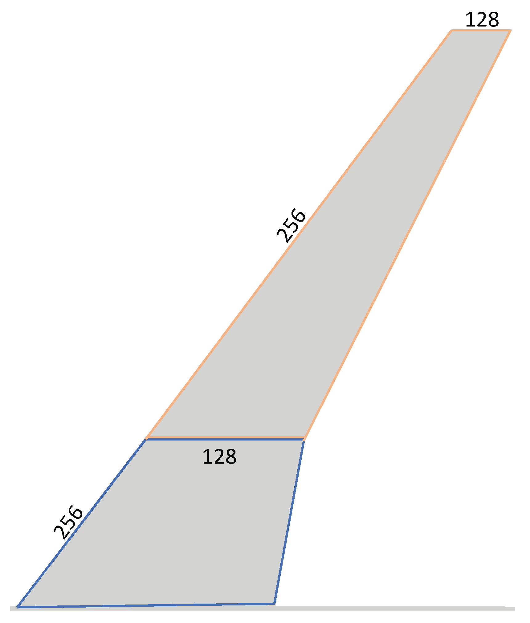
Prior to the training of the hybrid ROM, the numerical data need to be preprocessed. Due to the discretization of the wing suction side, the c p -distribution on the wing is represented by 168,686 data points. Therefore, in the first step, the size of the data is reduced by linear interpolation. The surface of the wing is divided into two parts, as shown in Figure 13. For each part, a grid with 256 nodes in the spanwise and 128 nodes in the chordwise direction is defined. The pressure distribution is linearly interpolated on the new grids. By stacking both grids together, the resulting pressure distribution resolution on the surface is defined by 128 × 512 ( 2 7 × 2 9 ) data points.
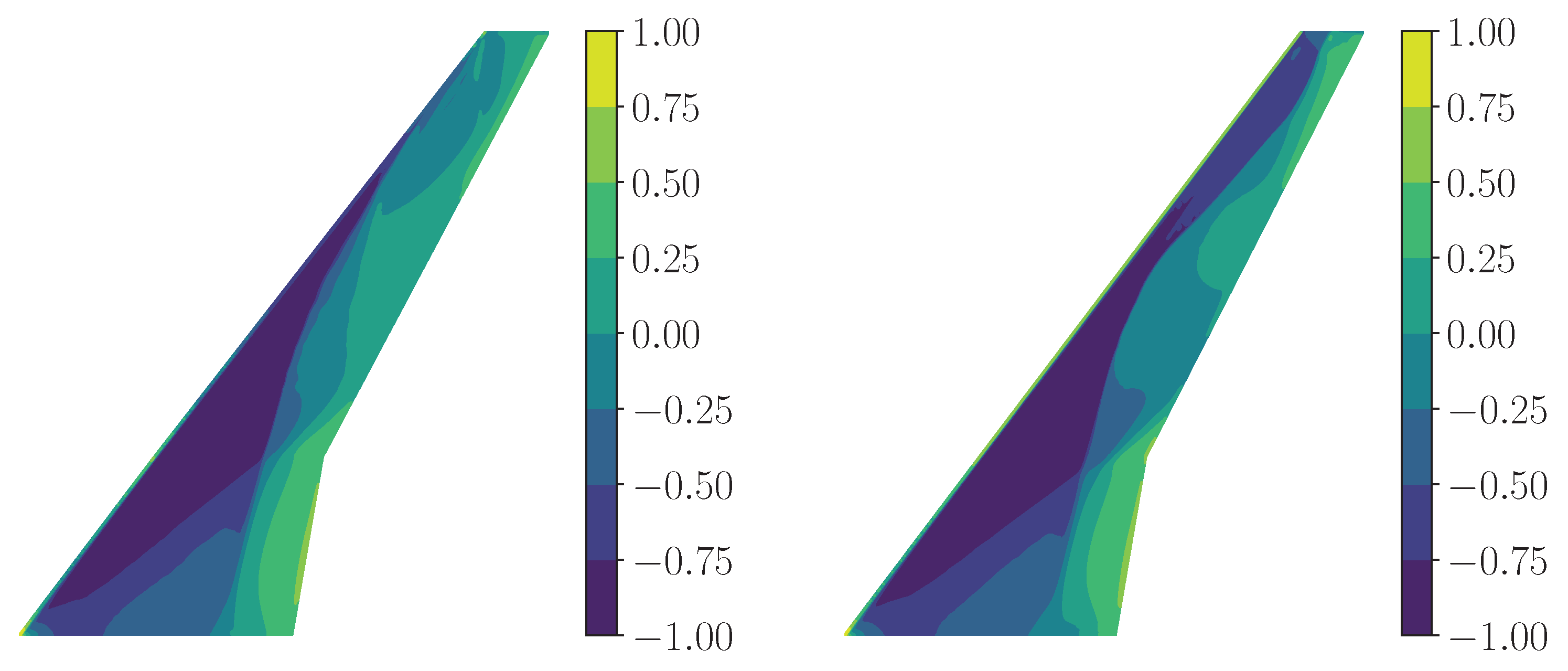
In Figure 14, the wing pressure distribution due to mode shape 11 in combination with the SAPRBS excitation is depicted at two individual time steps. Comparing the reduced spatial resolution with the original resolution visualized in Figure 11, a high level of spatial resolution is maintained. The characteristic λ -shaped two-shock pattern and changes in the spanwise pressure distribution, in particular in the mid-span and tip region, are still clearly visible.
In the same way as for the data representing the half-span model, both wings of the full-span model are separated in two parts, as shown in Figure 13. Therefore, the resulting pressure distribution is defined by 256 × 1024 ( 2 8 × 2 10 ) data points.
In the second step, all data sets are normalized to [−1,1] using the minimum and maximum pressure values of the numerical data sets ( c p , m i n , c p , m a x ).

4.2. Training of the Hybrid ROM

The training procedure of the hybrid ROM is divided into two consecutive steps. First, the CNN-AE is trained in order to reconstruct the available training data. Subsequent, the LSTM is trained based on the reduced data set encoded by the trained CNN-AE. In the following, two separate models for the symmetric and asymmetric mode shape c p -distributions are trained.
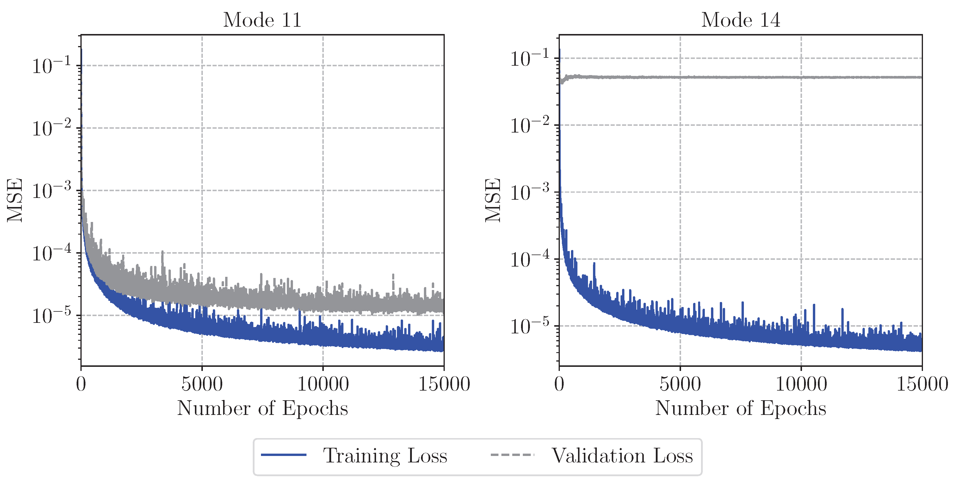
Prior to the training, the data set is split into training and validation data sets. Therefore, 80% of the c p -snapshots are used for training, whereas the remaining 20% are applied for validation and hyperparameter tuning. Based on a detailed parameter study, the following optimal hyperparameters have been identified: The CNN-AE is trained on batches, including 32 c p -snapshots each. For both the encoder and decoder, four convolution levels are applied. Considering both the data representing the symmetric and asymmetric mode shape related pressure distributions, the spatial resolution of the input data is reduced from 128 × 512 to 4 × 16 and 128 × 1024 to 4 × 32 , respectively. The channel size is increased from 3 to 512. By passing the FC layer, the latent size is reduced from 512 and 1024 to 256 features, respectively. The initial learning rate is defined as 10 4 and the training of the CNN-AE is terminated after 15,000 epochs. During the training, the mean squared error (MSE) between the reference numerical data and the corresponding predictions is minimized. In Figure 15, the trends of the training and validation losses of the CNN-AEs for mode 11 and 14 are visualized, respectively. As shown, the training and validation loss of mode 11 show clear convergence trends, while the validation loss of mode 14 stays constant after an initial number of epochs.
For clarification, besides the examination of the convergence trends, a numerical c p -snapshot of the validation data set and the corresponding predictions of the CNN-AE are compared. In Figure 16 and Figure 17, a numerical c p -snapshot (left) and the corresponding prediction of the CNN-AE (middle) are visualized for mode shape 11 and mode shape 14, respectively. The error between the two c p -distributions is represented by the MSE on the wing surface, as depicted in Figure 16 and Figure 17 right. As shown, the MSE between the numerical and predicted data is very small on almost the entire surface, indicating a good performance quality of the CNN-AEs.
In the same way as for the training of the CNN-AE, 80% of the data points are applied for the training of the LSTM. The data are fed into the LSTM in sequences, including 32 data points each, whereas the batch size is defined as one. A stacked LSTM with three layers is applied, with each layer including 256 neurons. The initial learning rate is defined as 10 4 and the LSTM is also trained for 15,000 epochs. For performance evaluation, the trained hybrid ROM is applied to the validation data set using recurrent multi-step predictions.
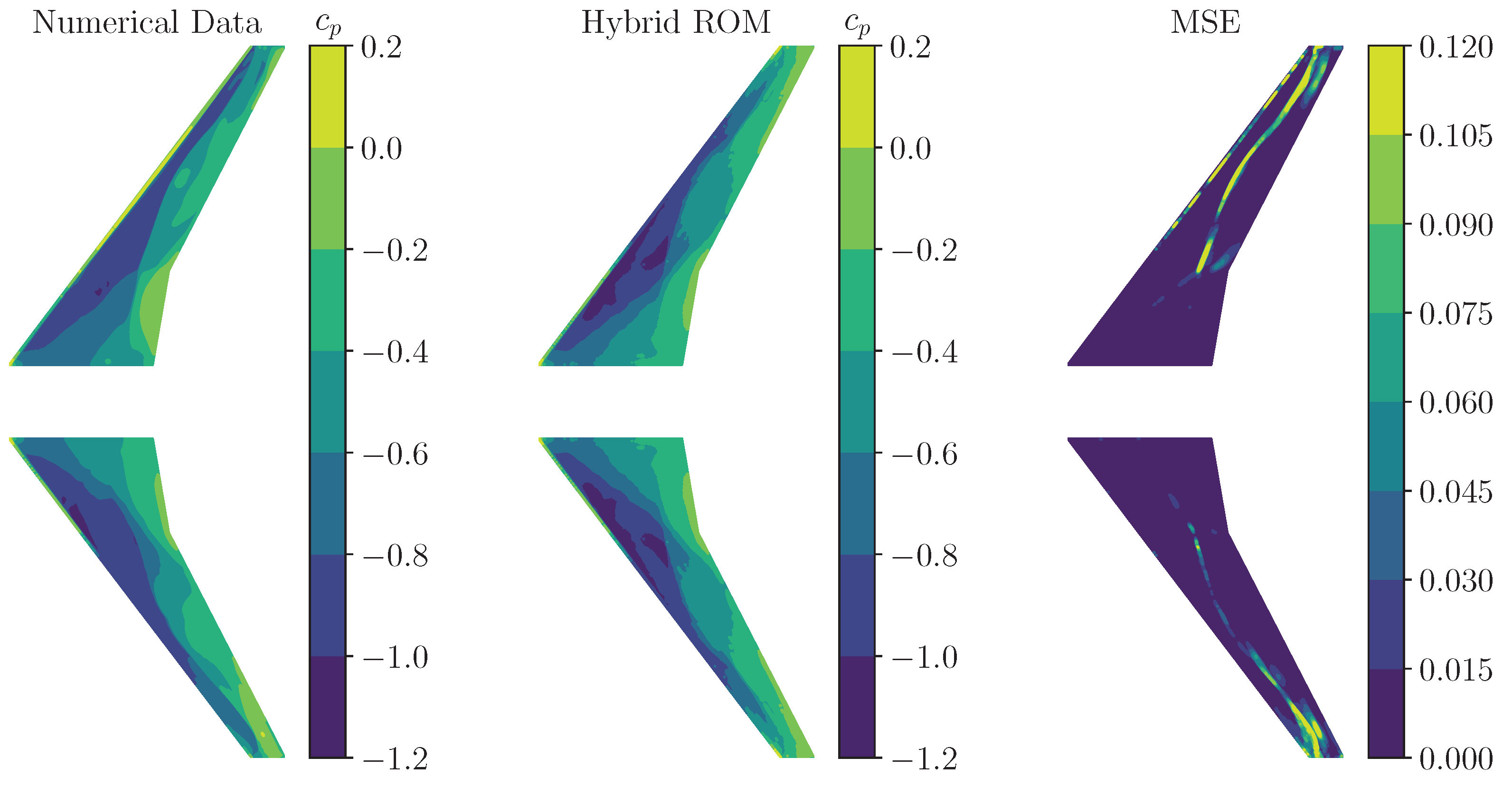
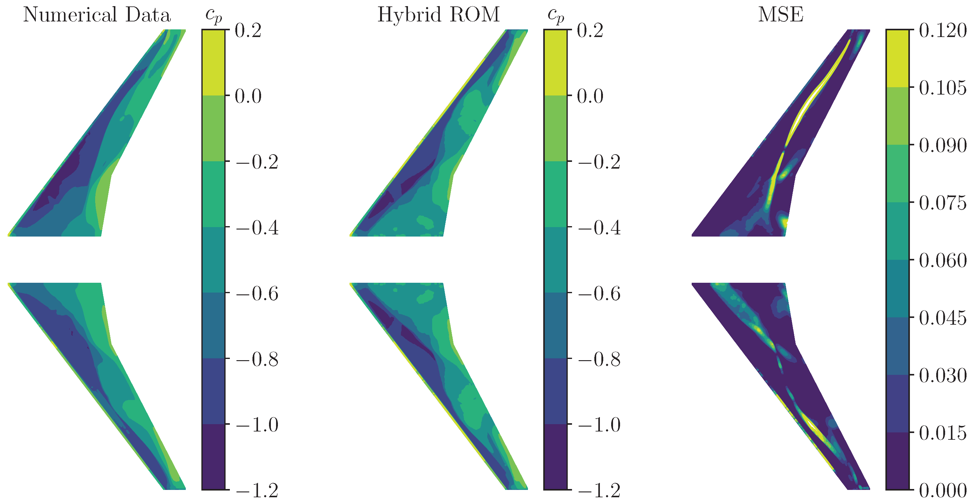
Therefore, an initial sequence including 32 c p -snapshots is presented to the trained model. As the prediction advances, the numerical data are successively replaced with predicted c p -snapshots. In Figure 18, a comparison between a numerical c p -snapshot (left) and the corresponding prediction of the hybrid ROM (middle) are visualized for the symmetric mode shape 11. Compared to the performance evaluation of the CNN-AE, slightly higher MSE values, especially at the position of the shock in the tip region, are indicated. However, the overall MSE on the wing is still sufficiently small.

4.3. Performance Evaluation

For the performance evaluation, the trained hybrid model is applied to predict the surface c p -distribution for the buffet condition in combination with mode shape deflections excited by a harmonic signal. The reduced frequency of the harmonic oscillation, which is defined as k r e d = 0.6, is chosen in order to represent a wing buffet frequency. The incidence amplitudes of the harmonic motions are defined equal to a reference scaling factor of f = [0.5%, 1%]. Due to the intense computational time, only a single oscillation period is computed with both the CFD solver and the trained hybrid ROM for the two test cases.
In the first step, the trained CNN-AEs are applied in order to reconstruct pressure distributions due to the harmonic excitation. In Figure 19, a comparison between a numerical c p -snapshot (left) and the corresponding, reconstructed c p -snapshot (middle) for mode shape 11 is visualized. Here, an excitation amplitude equal to f = 1% is considered. As shown, a good performance capability of the trained CNN-AEs is indicated by an overall small MSE on the wing suction side.
Following the performance evaluation of the trained CNN-AEs, in the second step the performance of the overall hybrid ROM is evaluated. Therefore, the test data sets are encoded and processed by the LSTM in a recurrent multi-step prediction mode. For the initialization of the multi-step predictions, a sequence of 32 encoded numerical c p -snapshots is provided to the LSTM. The corresponding initial 32 time steps of the harmonic excitation signal, defining the amplitudes of the deformation, are concatenated with the pressure data.
In order to evaluate the performance of the hybrid ROM, chordwise c p -distributions as modeled by the hybrid ROM are compared to the reference numerical c p -distributions. Therefore, two different spanwise positions η = [70%, 80%], which indicate distinct differences in the pressure distribution, are considered. The c p -distributions are defined at two different time steps included in the multi-step predictions. It has to be mentioned that, for mode shape 14, only the wing starboard side is considered. In Figure 20 and Figure 21, a comparison of the modeled and simulated c p -distributions for mode shapes 11 and 14 are visualized, respectively. As shown in Figure 20, the hybrid ROM is able to capture the trends of the pressure distribution of mode 11 at both spanwise positions. However, moderate deviations in the shock position are indicated, especially as the time step of the multi-step prediction advances. Focusing on the data comparison of mode 14 provided in Figure 21, larger deviations, especially in the level of shock intensity, compared to the mode 11 test case are shown. Similar to the predictions of mode 11, the c p -distributions at the advanced time step define a challenge for the hybrid ROM. The exact cause of the larger deviations observed for mode 14 could not be clearly identified; however, one possible explanation is the more complex structural deformation associated with this mode. As shown in Figure 9, the asymmetric wing bending mode may be more challenging for the hybrid ROM to accurately capture, although further investigations are required to confirm this hypothesis. Additionally, once the model uses its own predicted c p snapshots as input instead of numerical reference data, errors can accumulate and the rate of deviation may increase to some extent due to the propagation of artificial inputs. However, although deviations between the CFD and the hybrid ROM solutions are indicated, the overall trend of the shock position and the overall spanwise c p -distribution are captured by the proposed ROM.
In addition to the performance evaluation by means of comparing the chordwise c p -distribution, a comparison of the surface c p is provided for both test cases at the considered time step t = 2 (see Figure 20 and Figure 21). In Figure 22 and Figure 23, a comparison of surface c p for the mode 11 test cases with f = 1% and f = 0.5% is visualized, respectively. In Figure 24 and Figure 25, the corresponding surface c p distributions of mode shape 14 for both test cases are compared to the reference CFD solution. As shown in Figure 22, Figure 23, Figure 24 and Figure 25, the hybrid ROM is able to capture the c p -distributions to a sufficient extent. Moderate deviations in the overall MSE are indicated, which correspond to the results presented in Figure 20 and Figure 21.

4.4. Computational Efficiency

Within this last section, the reduction in computational costs by applying the proposed ROM in the framework of an aeroelastic analysis compared to URANS simulations is quantified.
Each numerical simulation with the DLR-TAU solver has been performed on the SuperMUC-NG of the Leibniz Supercomputing Center. For the half-span model, 10 nodes with 48 cores each have been applied, resulting in a total number of 480 cores. In contrast, for the simulation of the full-span model, 16 nodes with 48 cores (=768 cores) have been selected. The training, validation and test computations of the hybrid ROM have been conducted on a workstation equipped with an Intel Xeon W-2295 3 GHz processor. For comparability, only a single CPU core has been applied. Therefore, the following CPU hours represent wall clock times for each individual simulation.
In the framework of an aeroelastic analysis, a set of approximately 50 symmetric and asymmetric modes needs to be analyzed using URANS computations. Further, a fair amount of parameter variations, covering the frequency and amplitude range of interest, would be needed. Considering frequencies of k r e d , E x = [0.2:0.1:0.8] and a minimum number of two amplitude variations f = [0.5%, 1%], 16 simulations must be conducted for each respective symmetric and asymmetric mode. Therefore, in the following, a comparison between the application of the hybrid ROM in contrast to the fully resolved URANS simulations is given. To summarize the CPU time of the hybrid ROM, the SAPRBS simulations, the training of the ROM, the CFD computations of the initial input solutions and the application time of the ROM on the test data set are required. In contrast, the CPU time of the URANS simulations includes the CFD simulations of all required test cases.
Considering the half-span model simulations, the SAPRBS simulations for the generation of the training data set takes approximately 40 h, which equals a total computational time of around 19,200 (=40 × 480) CPU hours. The training of both the CNN-AE and the LSTM is summed up to approximately 40 CPU hours on the workstation. For the simulation of the initialization solution, approximately 4800 (=10 × 480) CPU hours are required. As a last step, the application of the trained ROM on the test data set is accomplished within 0.03 CPU hours. In contrast, the full URANS simulation comes up with a total of approximately 10,000 CPU hours for each frequency–amplitude variation. Here, 10,000 CPU hours are assumed as an average computational time, keeping in mind that each frequency is characterized by a different number of resolved time steps.
Focusing on the simulations of the asymmetric mode shapes, the generation of the training data set required approximately 76,800 (=100 × 768) CPU hours, whereas the training of the CNN-AE and LSTM is summed up to almost 60 CPU hours. For the computation of the initialization solution, approximately 11,520 (=15 × 768) CPU hours are necessary, whereas the application of the trained ROM is accomplished within 0.04 CPU hours. In order to simulate the reference full-order URANS solution, an average of 20,000 CPU for each test case is required (Table 2).
Considering a number of 16 parameter variations for each respective mode, the computational time of the hybrid ROM for one symmetric and asymmetric mode sums up to approximately 25,000 and 89,000 CPU hours, respectively. In contrast, the full URANS computations of the symmetric and asymmetric modes require around 16 × 10 4 and 32 × 10 4 CPU hours. Therefore, a reduction in computational time by one order of magnitude is possible. However, if the CPU hour for the training data set simulations are neglected, the computational time can be reduced by up to three orders of magnitude.

5. Conclusions

Within the present study, a hybrid deep learning model based on a convolutional autoencoder (CNN-AE) and a long short-term memory (LSTM) neural network has been applied for the prediction of wing buffet pressure distributions due to eigenmode-based structural deflections. The structural deflections have been imposed during an already established buffet instability in order to generate a highly nonlinear flow field. As a test case, the NASA Common Research Model (CRM) configuration has been selected. Based on the FERMAT structural model, a symmetric and an asymmetric wing-bending mode shape have been implemented and simulated. For the generation of the training data set, forced-motion CFD simulations of the mode shapes have been computed. In order to evaluate the performance capability of the trained hybrid ROM, the ROM is applied to predict buffet pressure distributions due to a harmonic excitation of the considered mode shapes. A comparison of the buffet loads as predicted by the hybrid ROM with the reference numerical solution shows that the proposed ROM is able to capture the trends of the pressure distributions of both the symmetric and asymmetric mode shapes. The demonstrated approach offers a computationally efficient and accurate tool for predicting unsteady aerodynamic loads, making it particularly valuable for future aeroelastic design studies and active flow control strategies. By significantly reducing the computational cost while maintaining high fidelity, the presented methodology can enable faster design iterations and improved unsteady load assessments for next-generation aircraft configurations.

Author Contributions

Conceptualization, R.Z., M.Z. and C.B.; methodology, R.Z. and M.Z.; software, R.Z. and M.Z.; validation, R.Z., M.Z. and C.B.; formal analysis, C.B.; investigation, R.Z.; resources, R.Z. and M.Z.; data curation, R.Z. and M.Z.; writing—original draft preparation, R.Z. and M.Z.; writing—review and editing, C.B.; visualization, R.Z.; supervision, C.B.; project administration, C.B.; funding acquisition, C.B. All authors have read and agreed to the published version of the manuscript.

Funding

The funding of the presented work within the Deutsche Forschungsgemeinschaft (DFG, German Research Foundation) framework of the research unit FOR 2895 (Unsteady flow and interaction phenomena at high speed stall conditions), subproject TP7, grant number BR1511/14-2 is gratefully acknowledged.

Data Availability Statement

The data presented in this study are available on request from the corresponding author.

Acknowledgments

The Gauss Centre of Supercomputing e.V. is gratefully acknowledged for funding this project by providing computing time on the SuperMUC-NG at Leibniz Supercomputing Centre. In addition, the authors thank the Institute of Aerodynamics and Gas Dynamics of the University of Stuttgart, in particular Maximilian Ehrle, for providing the numerical grid of the CRM.

Conflicts of Interest

The authors declare no conflicts of interest.

References

  1. Sator, F.; Timme, S. Delayed Detached-Eddy Simulation of Shock-Buffet on Half Wing-Body Configuration. AIAA J. 2016, 55, 1230–1240. [Google Scholar] [CrossRef]
  2. Iovnovich, M.; Raveh, D.E. Numerical Study of Shock Buffet on Three-Dimensional Wings. AIAA J. 2014, 53, 449–463. [Google Scholar] [CrossRef]
  3. Paladini, E.; Dandois, J.; Sipp, D.; Robinet, J. Analysis and Comparison of Transonic Buffet Phenomenon over Several Three-Dimensional Wings. AIAA J. 2018, 57, 1–18. [Google Scholar] [CrossRef]
  4. Koike, S.; Ueno, M.; Nakakita, K.; Hashimoto, A. Unsteady Pressure Measurements of Transonic Buffet on the NASA Common Research Model. In Proceedings of the 34th AIAA Aplied Aerodynamic Conference, AIAA-2016-4044, Washington, DC, USA, 13–17 June 2016. [Google Scholar] [CrossRef]
  5. Kou, J.; Zhang, W. Data-Driven Modeling for Unsteady Aerodynamics and Aeroelasticity. Prog. Aerosp. Sci. 2021, 125, 110725. [Google Scholar] [CrossRef]
  6. Kou, J.; Zhang, W.; Yin, M. Novel Wiener Models with a Time-Delayed Nonlinear Block and Their Identification. Nonlinear Dyn. 2016, 85, 2389–2405. [Google Scholar] [CrossRef]
  7. Silva, W. Application of Nonlinear Systems Theory to Transonic Unsteady Aerodynamic Responses. J. Aircr. 1993, 30, 660–668. [Google Scholar] [CrossRef]
  8. Glaz, B.; Liu, L.; Friedmann, P.P. Reduced-Order Nonlinear Unsteady Aerodynamic Modeling Using a Surrogate-Based Recurrence Framework. AIAA J. 2010, 48, 2418–2429. [Google Scholar] [CrossRef]
  9. Mannarino, A.; Mantegazza, P. Nonlinear Aeroelastic Reduced Order Modeling by Recurrent Neural Networks. J. Fluids Struct. 2014, 48, 103–121. [Google Scholar] [CrossRef]
  10. Zhang, W.; Kou, J.; Wang, Z. Nonlinear Aerodynamic Reduced-Order Model for Limit-Cycle Oscillation and Flutter. AIAA J. 2016, 54, 3304–3311. [Google Scholar] [CrossRef]
  11. Winter, M.; Breitsamter, C. Reduced-Order Modeling of Unsteady Aerodynamic Loads Using Radial Basis Function Neural Networks. In Proceedings of the 63rd Deutscher Luft- und Raumfahrtkongress, DGLR, Augsburg, Germany, 16–18 September 2014. [Google Scholar]
  12. Winter, M.; Breitsamter, C. Nonlinear Identification via Connected Neural Networks for Unsteady Aerodynamic Analysis. Aerosp. Sci. Technol. 2018, 77, 802–818. [Google Scholar] [CrossRef]
  13. Zahn, R.; Winter, M.; Zieher, M.; Breitsamter, C. Application of a Long Short-Term Memory Neural Network for Modeling Transonic Buffet Aerodynamics. Aerosp. Sci. Technol. 2021, 113, 106652. [Google Scholar] [CrossRef]
  14. Timme, S. Global Instability of Wing Shock-Buffet Onset. J. Fluid Mech. 2020, 885, A37. [Google Scholar] [CrossRef]
  15. Ohmichi, Y.; Ishida, T.; Hashimoto, T. Modal Decomposition Analysis of Three-Dimensional Transonic Buffet Phenomenon on a Swept Wing. AIAA J. 2018, 56, 3938–3950. [Google Scholar] [CrossRef]
  16. Chandon, M.; Levinski, O.; Altaf, A.; Carrese, R.; Marzocca, P. Aircraft Transonic Buffet Load Prediction using Artificial Neural Networks. In Proceedings of the 59rd AIAA Structures, Structural Dynamics and Materials Conference, AIAA-2019-0763, San Diego, CA, USA, 7–11 January 2019. [Google Scholar] [CrossRef]
  17. Afshar, Y.; Bhatnagar, S.; Pan, S.; Duraisamy, K.; Kaushik, S. Prediction of Aerodynamic Flow Fields Using Convolutional Neural Networks. Phys. Fluids 2019, 64, 525–545. [Google Scholar] [CrossRef]
  18. Sekar, V.; Jiang, Q.; Shu, C.; Khoo, B.C. Fast Flow Field Prediction over Airfoils Using Deep Learning Approach. Phys. Fluids 2019, 31, 057103. [Google Scholar] [CrossRef]
  19. Li, Y.; Chang, J.; Wang, Z.; Kong, C. An Efficient Deep Learning Framework to Reconstruct the Flow Field Sequences of the Supersonic Cascade Channel. Phys. Fluids 2021, 33, 056106. [Google Scholar] [CrossRef]
  20. Hasegawa, K.; Fukami, K.; Muarata, T.; Fukagata, K. Machine-Learning-Based Reduced-Order Modeling for Unsteady Flows Around Bluff Bodies of Various Shapes. Theor. Comput. Fluid Dyn. 2020, 34, 367–383. [Google Scholar] [CrossRef]
  21. Nakamura, T.; Fukami, K.; Hasegawa, K.; Nabae, Y.; Fukagata, K. Convolutional Neural Network and Long Short-Term Memory Based Reduced Order Surrogate for Minimal Turbulent Channel Flow. Phys. Fluids 2021, 33, 025116. [Google Scholar] [CrossRef]
  22. Liu, Z.; Han, R.; Zhang, M.; Zhang, Y.; Zhou, H.; Wang, G.; Chen, G. An Enhanced Hybrid Deep Neural Network Reduced-Order Model For Transonic Buffet Flow Prediction. Aerosp. Sci. Technol. 2022, 126, 107636. [Google Scholar] [CrossRef]
  23. Klimmek, T. Parametric Set-up of a Structural Model for FERMAT Configuration Aeroelastic and Loads Analysis. J. Aeroelast. Struct. Dyn. 2014, 3, 31–49. [Google Scholar]
  24. Goodfellow, I.; Bengio, Y.; Courville, A. Deep Learning, 1st ed.; MIT Press: Cambridge, MA, USA, 2016; ISBN 978-0-2620-3561-3. [Google Scholar]
  25. Rosov, V.; Breitsamter, C. Data-Driven Prediction of Unsteady Pressure Distributions Based on Deep Learning. J. Fluids Struct. 2021, 104, 103316. [Google Scholar] [CrossRef]
  26. Rumelhart, D.E.; Hinton, G.E.; Williams, R.J. Learning Representations by Back-Propagating Errors. Nature 1986, 323, 533–536. [Google Scholar] [CrossRef]
  27. Hochreiter, S.; Schmidhuber, J. Long Short-Term Memory. Neural Comput. 1997, 9, 1735–1780. [Google Scholar] [CrossRef]
  28. Hochreiter, S.; Bengio, Y.; Fransconi, P.; Schmidhuber, J. Gradient Flow in Recurrent Nets: The Difficulty of Learning Long-Term Dependencies. In A Field Guide to Dynamical Recurrent Neural Networks; IEEE: Piscataway, NJ, USA, 2003. [Google Scholar] [CrossRef]
  29. Werbos, P.J. Backpropagation Through Time: What it does and how to do it. Proc. IEEE 1990, 78, 1550–1560. [Google Scholar] [CrossRef]
  30. Kingma, D.P.; Ba, J.L. Adam: A Method for Stochastic Optimization. In Proceedings of the International Conference on Learning Representations, San Diego, CA, USA, 7–9 May 2015; Volume 12. [Google Scholar]
  31. Ioffe, S.; Szegedy, C. Batch Normalization: Accelerating Deep Network Training by Reducing Internal Covariate Shift. In Proceedings of the 32nd International Conference on Machine Learning, Lille, France, 6–11 July 2015; Volume 37, pp. 448–456. [Google Scholar]
  32. Ehrle, M.; Waldmann, A.; Lutz, T.; Krämer, E. Simulation of Transonic Buffet with an Automated Zone DES Approach. CEAS Aeronaut. J. 2020, 11, 1025–1036. [Google Scholar] [CrossRef]
  33. Lutz, T.; Gansel, P.P. Going for Experimental and Numerical Unsteady Wake Analyses Combined with Wall Interference Assessment by Using the NASA CRM-Model in ETW. In Proceedings of the 51st AIAA Aerospace Sciences Meeting, AIAA-2013-871, Grapevine, TX, USA, 7–10 January 2013. [Google Scholar] [CrossRef]
  34. Spalart, P. Strategies for Turbulence Modeling and Simulations. J. Heat Fluid Flow 2000, 21, 252–263. [Google Scholar] [CrossRef]
  35. Togiti, V.; Eisfeld, B.; Brodersen, O. Turbulence Model Study For the Flow Around the NASA Common Research Model. J. Aircr. 2014, 54, 1331–1343. [Google Scholar] [CrossRef]
  36. Illi, S.; Fingskes, C.; Lutz, C.; Krämer, E. Transonic Tail Buffet Simulations for the Common Research Model. In Proceedings of the 31st AIAA Applied Aerodynamics Conference AIAA 2013-2510, San Diego, CA, USA, 24–27 June 2013. [Google Scholar] [CrossRef]
  37. Winter, M. Nonlinear Aerodynamic Reduced-Order Modeling Using Neuro-Fuzzy Approaches. Ph.D. Thesis, Technical University of Munich, Garching, Germany, 2021. [Google Scholar]
  38. Winter, M.; Breitsamter, C. Application of Unsteady Aerodynamic Reduced-Order Modeling Techniques to a Complex Configuration. In Proceedings of the 17th International Forum on Aeroelasticity and Structural Dynamics, Como, Italy, 25–28 June 2017. IFASD Paper 2017-217. [Google Scholar]
  39. Nelles, O. Nonlinear System Identification: From Classical Approaches to Neural Networks and Fuzzy Models, 1st ed.; Springer: Berlin/Heidelberg, Germany, 2001; ISBN 978-3-662-04323-3. [Google Scholar]
Figure 1. Architecture of the LSTM cell including the characteristic gate structure.
Aerospace 12 00415 g001
Figure 2. Architecture of the hybrid deep learning model.
Aerospace 12 00415 g002
Figure 3. Concatenation of deformation q and surface c p .
Aerospace 12 00415 g003
Figure 4. Geometry of the NASA CRM wing/body/horizontal-tail configuration. (a) Isometric view. (b) Top view. (c) Front view. (d) Back view.
Aerospace 12 00415 g004
Figure 5. Hybrid numerical grid of the CRM configuration.
Aerospace 12 00415 g005
Figure 6. Comparison of numerical and experimental c ¯ p at a spanwise position of η = 60% ( M a = 0.85 , R e = 30 × 10 6 , α = 5°).
Aerospace 12 00415 g006
Figure 7. Pressure coefficient ( c p ) contour plots showing the buffet cycle of the NASA CRM ( M a = 0.85 , R e = 30 · 10 6 , α = 5 ° ). T B u f f e t refers to the buffet period. (a) Full buffet cycle. (b) Surface pressure coefficient at η = 60 % . (c) Surface pressure coefficient at η = 70 % . (d) Surface pressure coefficient at η = 80 % .
Aerospace 12 00415 g007
Figure 8. Comparison of the original structural FEM (a) and the reduced structural FEM (b) [37].
Aerospace 12 00415 g008
Figure 9. Selected structural eigenmode-based surface deformations of the FERMAT-C2 configuration (red) and the non-deformed CRM geometry (gray). (a) First symmetric wing-bending mode. (b) First asymmetric wing-bending mode.
Aerospace 12 00415 g009
Figure 10. SAPRBS time series for the forced-motion excitation of the mode shapes.
Aerospace 12 00415 g010
Figure 11. Pressure coefficient ( c p ) contour plots showing the SAPRBS excitation of symmetric mode 11 ( M a = 0.85 , R e = 30 · 10 6 , α = 5 ° ).
Aerospace 12 00415 g011
Figure 12. Pressure coefficient ( c p ) contour plots showing the SAPRBS excitation of antisymmetric mode 14 ( M a = 0.85 , R e = 30 · 10 6 , α = 5 ° ).
Aerospace 12 00415 g012
Figure 13. Separation of the wing suction side into two parts for surface c p interpolation.
Aerospace 12 00415 g013
Figure 14. Interpolated and normalized surface c p resolution on the wing suction side at two selected time steps (symmetric mode 11, SAPRBS excitation).
Aerospace 12 00415 g014
Figure 15. Convergence trends of training and validation losses of both trained CNN-AEs (mode 11 (left), mode 14 (right)).
Aerospace 12 00415 g015
Figure 16. Comparison of a numerical c p -snapshot (left) and a c p -snapshot obtained by the trained CNN-AE (middle) (mode 11, SAPRBS excitation). The corresponding MSE is shown on the (right) wing surface.
Aerospace 12 00415 g016
Figure 17. Comparison of a numerical c p -snapshot (left) and a c p -snapshot obtained by the trained CNN-AE (middle) (mode 14, SAPRBS excitation). The corresponding MSE is shown on the (right) wing surface.
Aerospace 12 00415 g017
Figure 18. Comparison of a numerical c p -snapshot (left) and a c p -snapshot obtained by the trained hybrid ROM (middle) (mode 11, SAPRBS excitation). The corresponding MSE is shown on the (right) wing surface.
Aerospace 12 00415 g018
Figure 19. Comparison of a numerical c p -snapshot (left) and a c p -snapshot obtained by the trained CNN-AE (middle) (mode 11, harmonic excitation, f = 1%). The corresponding MSE is shown on the (right) wing surface.
Aerospace 12 00415 g019
Figure 20. Comparison of c p -distributions at two spanwise positions of η = [70%, 80%] at two individual time steps t of the multi-step prediction results (mode 11, harmonic excitation, f = [1%, 0.5%]).
Aerospace 12 00415 g020
Figure 21. Comparison of c p -distributions at two spanwise positions of η = [70%, 80%] at two individual time steps t of the multi-step prediction results (mode 14, harmonic excitation, f = [1%, 0.5%]).
Aerospace 12 00415 g021
Figure 22. Comparison of a numerical c p -snapshot (left) and a c p -snapshot obtained by the trained hybrid ROM (middle) (mode 11, harmonic excitation, f = 1%, t = 2). The corresponding MSE is shown on the (right) wing surface.
Aerospace 12 00415 g022
Figure 23. Comparison of a numerical c p -snapshot (left) and a c p -snapshot obtained by the trained hybrid ROM (middle) (mode 11, harmonic excitation, f = 0.5%, t = 2). The corresponding MSE is shown on the (right) wing surface.
Aerospace 12 00415 g023
Figure 24. Comparison of a numerical c p -snapshot (left) and a c p -snapshot obtained by the trained hybrid ROM (middle) (mode 14, harmonic excitation, f = 1%, t = 2). The corresponding MSE is shown on the (right) wing surface.
Aerospace 12 00415 g024
Figure 25. Comparison of a numerical c p -snapshot (left) and a c p -snapshot obtained by the trained hybrid ROM (middle) (mode 14, harmonic excitation, f = 0.5%, t = 2). The corresponding MSE is shown on the (right) wing surface.
Aerospace 12 00415 g025
Table 1. Geometric properties of the CRM configuration.
QuantitySymbolValue
Wing reference area A r e f 0.280 m2
Wing spanb1.586 m
Mean aerodynamic chord c r e f 0.189 m
Aspect ratio A R 9
Quarter-chord sweep angle ϕ 0.25 35°
Table 2. Comparison of CPU hours per case between URANS simulations and the hybrid ROM approach.
Hybrid ROM
Casen.o.p.URANSTraining Data SetInitialTrainingTotal
symmetric110,00019,20048004024,040
symmetric16160,00019,200480064024,640
asymmetric120,00076,80011,5206088,380
asymmetric16320,00076,80011,52096089,280
Disclaimer/Publisher’s Note: The statements, opinions and data contained in all publications are solely those of the individual author(s) and contributor(s) and not of MDPI and/or the editor(s). MDPI and/or the editor(s) disclaim responsibility for any injury to people or property resulting from any ideas, methods, instructions or products referred to in the content.