1. Introduction
In recent years, increasingly powerful machine learning methods have been developed that can solve more and more tasks thanks to the increasingly available computing power. This also makes machine learning methods interesting for use in aviation. For use in such an environment, it must be possible to demonstrate the reliability with which the system that uses machine learning methods functions. A common approach here is to demand a suitable minimum reliability depending on the application (see
Section 1.1). This distinguishes the use in aviation from many other applications: it is not enough for a system to function reliably; it must also be possible to prove and document this as part of the certification. This also justifies an additional analysis effort, as use is only possible at all after successful certification. For this, it is not sufficient to only check the created model for correctness at discrete test points, as the behaviour between these points is not checked (see
Section 1.3). If the number of test points could be arbitrarily increased, this problem could be solved. However, this is not possible for real applications, and the number of data points required increases considerably with the number of variables, due to the curse of dimensionality. Other further information is therefore required. How this information can be obtained and integrated into the validation process is presented and discussed in this method study. In order to make the validation process sufficiently short and thus manageable, it is suggested to use the symbolic regression method to create the models, as this is particularly useful for finding compact models. This work deals, in particular, with physical models, as additional information is available for these models as they have to be dimensionally homogeneous.
1.1. Reliability Requirements Based on the Planned Utilization
The requirements for reliability are not dependent on the specific model but on the planned utilization. This means that the exact same model can be sufficient for one application, but not for another. For example, in the Certification Specifications for Large Aeroplanes (CS-25, [
1] (p. 779)) this is defined on a very high level for the overall system: depending on the severity of a failure, an acceptable possibility is defined which must not be exceeded. Therefore, the criticality of every system has to be determined, which results in the acceptable failure possibility. This is also an approach that the EASA currently follows in developing certification strategies for AI/ML systems. The Artificial Intelligence Concept Paper [
2] proposes different levels of requirements depending on the planned use case. Determining the safety requirements for a model based on its planned use seems promising and is therefore pursued in this work.
The reason why planned utilization is the main driver for the definition of criticality can be seen in the following three examples with different criticality, which are applications for machine learning models:
Thermals can be used to extend the flight time of an aircraft. Finding these thermals and encircling them is a difficult task, for which [
3] developed and demonstrated a system. This is a nice example for a non-critical system, as a backup strategy has to be implemented if no thermal is found, as it is also not guaranteed that a thermal will be available.
Another less critical application is the weather forecast for the next few days, shown, for example, by [
4], as due to the uncertainty of the state-of-the-art forecasts, mitigation techniques for incorrect forecasts are well known.
A possible highly critical system is the detection of wake vortex positions and strengths based on Lidar measurements, as shown by [
5]. Currently, the aircraft approaching an airport are temporally separated based on the expected wake turbulence, which is mass dependent. If a lighter aircraft approaches behind a heavier one, the wake vortexes can be a very hazardous risk. Therefore, the runway is closed for a certain time to ensure the vortex is sufficiently weakened by friction. If this time could be reduced by measuring strength, the capacity of the runway can be increased, but it has to be ensured that the measurement is correct to not endanger any aircraft.
These examples show that the effects of an error in a machine learning model or any other model do not depend on the type of model, but on its use.
1.2. Verification and Validation of Machine Learning Models
The verification and validation of machine learning models is part of current research. The available methods determine how well reliability can be determined. The more safety-critical the application is, the more soundly the reliability of the model must be able to be determined.
1.2.1. State of the Art
The basis for every machine learning model is the data with which it is trained on. The model can only learn what is included in the data and it has to be ensured that no undesirable information, e.g., systematic measurement errors, is included. This also limits the achievable accuracy of a machine learning model [
6]. For regression tasks, Budach et al. [
7] found that the quality dimensions with the largest impact are completeness, feature accuracy, and target accuracy. This means that no relevant values should be missing and that feature values as well as the target values should equal their respective ground truths.
Different types of tests to estimate the accuracy and the reliability of the model output have been developed. For the accuracy, many different metrics were developed, which can be used to evaluate the deviation of the model output from the desired value. One of the most famous metrics is the root-mean-square error, which penalizes particularly large deviations disproportionately. An extensive survey of metrics can be found in Botchkarev [
8]. Best practice for the model creation and the evaluation of the accuracy is to split the data set into at least two, preferably three, parts. The biggest part is used as training data and the smaller part is used for assessing the accuracy during the current training step. A third part can be used to determine the accuracy after the model generation is finished. This split is performed to evaluate the model at points which were not used during the training to avoid the model only representing the training data correctly and not generalizing properly (the so-called overfitting).
Nevertheless, the number of data points is limited and therefore, methods were developed to estimate the overall error. This field of research is called uncertainty estimation. There are two main aspects: learning the estimated error or calculating the uncertainty. In real-world applications, the input data are uncertain, for example, as a result of sensor noise. This uncertainty also affects the model result, which is why it should also be learned and output by the model. The other aspect is to calculate the uncertainty of the error for the whole test data set. This helps to evaluate the model overall, but does not give the expected error for a single, unknown data point. A detailed explanation and discussion of uncertainty estimation techniques can be found in Gawlikowski et al. [
9].
For the reachability problem, which elaborates if there is a valid input for a given valid output, and the search of bounds, different algorithms were created. They are mostly search algorithms based on heuristics, as a complete evaluation is too computationally expensive (see also
Section 1.2.2). An overview can be found in Liu et al. [
10]. Another approach is to interpret the machine learning model. Many different approaches have been developed, a review can be found in Carvalho et al. [
11]. The biggest challenge in interpreting a model is that interpretability is difficult to formalise and therefore difficult to standardise. An extensive review of the literature on how to certify machine learning based safety-critical systems can be found in Tambon et al. [
12]. For the subfields of robust training, post-training robustness analysis, uncertainty estimation and ODD (out-of-distribution detection), explainability, verification, safe reinforcement learning, as well as direct certification, many different, mostly empirical, methods are discussed, but there is no recognisable consensus as to which method should be used for which problem in order to be able to carry out a conclusive review.
1.2.2. Limitations
Different limitations for verification and validation, especially for (deep) neural networks, have been found in the past. It could be proven that “given an NN and symbolic specifications of valid inputs and outputs, decide whether there is some valid input such that the corresponding output is valid […] is NP-hard for NN with output dimension one, a single hidden layer and simple specifications” [
13]. For this proof, the Rectified Linear Unit (ReLU) and the identity function were assumed as their activation functions. The complexity of the reachability problem using other activation functions is discussed in Wurm [
14]. Among other things, this problem is is described as NP-hard for sigmoidal functions. Also, it could be proven that verifying properties in deep neural networks with ReLUs is NP-complete [
15]. For Message-Passing Neural Networks, it is shown by Sälzer and Lange [
16] that no formal verification is even possible.
Not only is the verification of a finalized neural network at least NP-hard, the training is also NP-hard [
17] or even
-complete [
18]. This means that it is unlikely that an algorithm can be found which guarantees that the weights are set optimally in a reasonable runtime. If this cannot be guaranteed, this means it cannot be guaranteed that a data set is approximated correctly; therefore, a validation solely based on the training process is unlikely.
1.3. Problem Statement: Validation of Machine Learning Models in Safety-Critical Domains
In safety-critical domains, it has to be proven that the overall system does not fail with more than a given probability. Depending on where the machine learning model is used in the overall system, even single wrong results are not acceptable or it must be at least ensured that wrong results are not occurring more likely than a given probability.
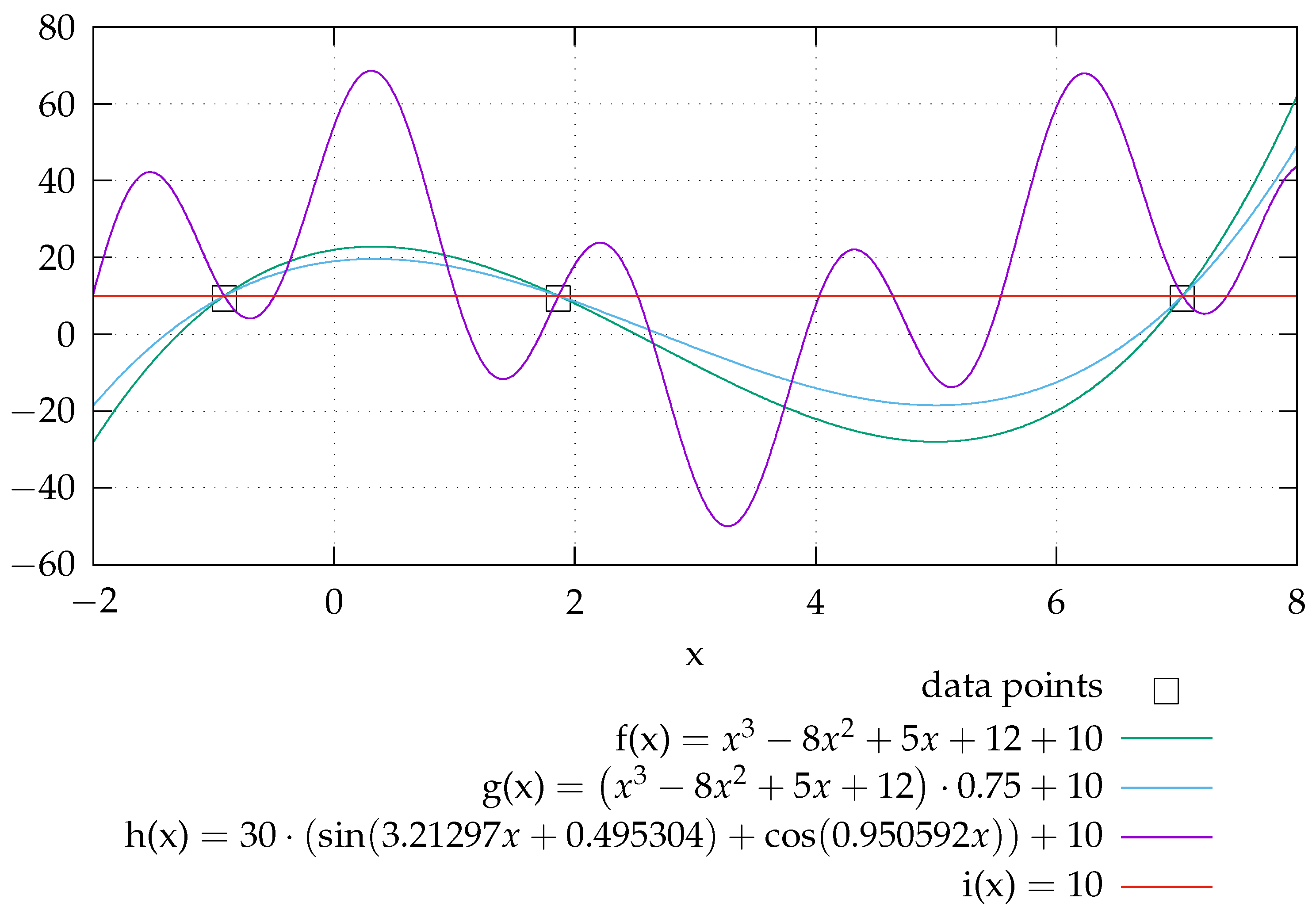
For real-world applications, the number of data points, and therefore the number of test points, is limited. If these are used to evaluate the model accuracy, this is always a discrete test. For continuous functions, the behaviour between these points remains untested. This is illustrated in
Figure 1. All graphs pass through the data points, but have a different behaviour in between. Based on the data points, it cannot be decided which formula models the behaviour correctly. Adding data points only reduces the interval size where the true behaviour is unknown. This variety can also be described as there are many distinct models that solve the problem equivalently, which is identified as “underspecification” in ML pipelines by D’Amour et al. [
19]. For derivated models, this is not a problem as the behaviour is justified by the derivation. Also, limitations or assumptions are made explicitly and are therefore known in detail.
2. Validation of Machine Learning Models Using Domain Knowledge
For the usage of machine learning models in safety-critical domains, where it is not possible to create an extreme amount of data points, the uncertainty of the behaviour between the test points has to be overcome. If a model is designed manually based on measured points, this problem stays the same; however, such models are widely used. Therefore, the question arose: what is the difference between a human expert designing a model and a machine learning approach?
2.1. Observation: Expert Approach
When designing a model manually, an appropriate approximation function based on the expected system behaviour is selected and tools are only used to fit the parameters. The same applies to the design of a neural network. Different architectures are compared with each other to find the best one for the given task. For the selection of appropriate approximation functions or network architectures as well as for the assessment of the found models, domain knowledge is used. This means that not only the given data points but also the expected behaviour is taken into account.
2.2. Symbolic Regression
A human expert selects promising functions and not a multitude of simple approximations which are combined. (For example a generic approach is an approximation using polynomials, as “According to the Weierstrass approximation theorem, every continuous function on a bounded closed interval [a, b] can be approximated arbitrarily well by polynomials in the metric space of the space
([a, b]), i.e., uniformly” [
20] (p. 665). This leads to extensive terms, but has the benefit that no specialized approach needs to be selected.) These promising functions are mostly combinations of elementary functions as they are easy to handle. (Elementary functions are functions “that can be realised by algebraic operations, concatenations and inversions from algebraic functions and the exponential function. This includes all rational functions, exponential and logarithmic functions, the trigonometric functions, and hyperbolic functions as well as their inverse functions” [
21] (p. 30) (translation by the authors).) If this is performed by a computer, it is called symbolic regression. Different approaches have been developed in the past, for example, to gain knowledge about scientific processes from data [
22], also using dimensionality analysis [
23,
24,
25]. However, the symbolic regression is considered NP-hard [
26]. Despite this, there are two main benefits: the model is represented by a closed-form analytical formula, and all elementary functions can be taken into account. The representation as a closed-form analytical formula leads to an easy implementation of the model and the model can be evaluated using the whole toolbox that the mathematical analysis offers. As all elementary functions can be directly incorporated into the model, there is no need to approximate them with simpler functions, which reduces the number of terms.
It is also possible to use domain knowledge during the search process. This knowledge is often used to narrow the search space, e.g., by limiting the available terms. This is called “Scientist-in-the-loop” by Keren et al. [
27]. However, the requirements that can be placed on the model are significantly limited by the fact that the evaluation of whether these requirements are met must be carried out thousands of times during the search for a model. Simple requirements, such as that a value must not be exceeded, can be checked quickly, but the determination of extreme values, for example, can easily become too time-consuming. During the search, models are created iteratively, for example, either by a tree search as described in Anselment et al. [
24], or by a genetic algorithm as described in Keren et al. [
27], which are evaluated and for which a decision must then be made as to whether they meet the requirements. However, it can happen that a model is invalid in the meantime, but in fact only the correctness of the final solution is relevant. This can be easily seen on a simple example. If
should be continuous, a model could be found in three steps:
(continuous for )
(not continuous for , pole at )
(continuous for )
In step one and three the requirement would be fulfilled, while in step two, it would not be. If the solution had been discarded in step two, the valid final solution would not have been found. Therefore, a procedure should be introduced for dealing with such interim solutions.
2.3. Verification of the Model
If the model cannot approximate the given test and validation points, it is not possible that the correct model has been found. This means that the quality of the approximation, e.g., measured by the root-mean-square error, needs to be sufficient.
2.4. Validation by Specifying the Expected Behaviour
From observing how models are created manually, it follows that the expected behaviour can fill in the missing information between data points. This procedure should be formalised by defining an area by an expert where the model output is expected to be within, which, in consequence, is called the “behaviour envelope”. This is inspired by the flight envelope of an aircraft: on one hand, it is proven that the structural strength is sufficiently high within these limits; on the other hand, it is necessary to ensure that flight planning and flight execution remain within this range in order to guarantee safe execution without requiring an exact determination of the load during each flight.
The expected behaviour is used to define an area in which the response of the model is plausible. If this can be ensured, it can be expected that the model represents the correct overall behaviour. The detailed definition of the model is performed by learning the parameters, but due to the fact that the general behaviour is within the limits, it can be assumed that between the test points, the model behaviour is as expected, whereby a limited number of test points is sufficient to ensure the overall behaviour. This is proposed as an approach to overcome underspecification. An example of this can be seen for h(x) in
Figure 1. If it is known that such a high frequency is not part of the system which should be modelled (e.g., because it is an inert system), this solution can be ruled out. Also, data quality plays an important role, as the behaviour envelope can ensure that the overall behaviour is correct, but the quality of the model is nevertheless dependent on the available data, as some variability within the envelope still remains.
The specification of a behaviour envelope differs from the classical requirements in engineering, which is used to define the objectives a system should cover under given circumstances. (Requirements engineering is defined as “Requirements engineering is the branch of engineering concerned with the real-world goals for, functions of, and constraints on systems. It also concerns the relationship of these factors to precise specifications of system behaviour and to their evolution over time and across families of related systems.” by [
28].) These goals are specific to every project and depend on the needs of the stakeholders. In contrast to this, the definition of a behaviour envelope is driven by the (physical) behaviour of the system and cannot be, except for the level of detail, negotiated. Nevertheless, to stay within the envelope for given inputs can be a requirement to be able to utilize a model.
2.4.1. Behaviour Envelope
For the definition of the behaviour envelope, the boundaries can be appraised. As a result of this, it is not mandatory to have in-depth detailed knowledge of the system (which would also counteract the data-driven approach), as the general behaviour of a system can be much easier understood. Possible constraints to define the envelope, for the function that represents the model as well as the respective gradient functions, can be the following:
Minimum and maximum values;
Turning points;
Oscillations;
Continuity or expected saltus;
Position of special points in relation to each other;
Not crossing a function in a given interval, e.g., .
The behaviour envelope can be justified as well as documented and also retraced at a later date, which is especially relevant for the certification of a model. For physical models, another justification also needs to be taken into account: “For physical equations to remain valid for any chosen unit system, each summand of such an equation must carry the same dimension. Equations which satisfy this property are called dimensionally homogeneous” [
29]. This means that the formula remains valid independently of the fundamental units chosen [
30] (p. 79). If this is not fulfilled, the model is broken by design, but this is just a necessary condition as this does not imply that the correct model has been found.
2.4.2. Verification That the Model Stays in the Behaviour Envelope
The main part is to ensure that the model stays within the defined behaviour envelope. The goal is to verify the model itself and not only the output values during the runtime, which is performed by comparing the output to another model that is often simple. Otherwise, the machine learning approach would not be necessary or the runtimes would be too long, so it is typically ensured that limits are not overrun but gradients are not available. Preferably the verification is performed in an analytical way; otherwise, the problem described in
Section 1.3 concerning the model behaviour between the test points arises again. The effort for an analytical investigation increases with the model size, which is why a compact model is preferred. This is particularly relevant if gradients are to be determined and analysed symbolically, as even powerful computers quickly reach their limits here. Since symbolic regression promises very compact models compared to other machine learning methods, especially in comparison with neural networks, it makes sense to use it here, even though the effort required to create the model initially seems higher.
2.5. Interim Conclusion
Ensuring the correctness of machine learning models is based on two pillars. One is to evaluate the error for a given set of test points to determine if the model predicts correctly at discrete points (verification of the model) and the other one is to ensure the correct overall behaviour by using domain knowledge which is used to define a behaviour envelope and then proving mathematically that the model stays within this limit (validation of the model). To be able to achieve this, a compact model, represented by a closed-form analytical formula, is necessary. This formula can be found by symbolic regression. As both the training of a neural network and symbolic regression are (at least) NP-hard—although it is possible that the analysis of the result of the symbolic regression is not NP-hard (this depends on the found formula)—it is proposed to shift the effort to the model generation in order to simplify the validation.
3. Example: Polar of a Schempp–Hirth Mini-Nimbus Sailplane
The described methodology is illustrated by a simple, aerospace-related example. A simple example has been chosen so that the methodology can be easily comprehended. As an example, the polar of a Schempp–Hirth Mini-Nimbus sailplane was selected. The Mini-Nimbus is a single-seated sailplane with a
wingspan built in a fibre composite construction and has commercially been available since 1977 [
31]. The values for the polar are taken from [
32]. A measurement error of
to
can be assumed. (In [
32], two measurement methods are mentioned with which the polars for three different sailplanes are measured. Sadly, Professor Eppler, who originally provided the data, passed away in 2021, so it is no longer possible to clarify which method was used to measure the Mini-Nimbus. However, it is most likely that the photogrammetric measurement method, which has the mentioned error, was used. [J. Wandinger, personal communication, 07 June 2024 [
32]].) This example was selected to demonstrate the approach on real data, but with a reasonable complexity. As it is usual in flight manuals for sailplanes, the airspeed
v is given in
and the rate of descent
in
.
3.1. Definition of Behaviour Envelope
At first, the behaviour envelope has to be specified, which can be characterized as follows:
Only interpolation between given data points, as an extrapolation is expected to be unreliable due to the non-linear behaviour of the aircraft aerodynamics (especially at low speeds because of the stall).
The polar is continuous.
The polar contains only one extremum (a minimum), which is at the speed of the best rate of descent.
For the best rate of descent, must be valid.
The polar has no saddle point.
The polar has no turning points, i.e., it is not superimposed by high-frequency oscillations.
The best L/D ratio (Lift-over-Drag ratio, see Equation (
1)) is above 25 (Schleicher K 8 [
33], timber construction with covering) and below 70 (eta [
34], best sailplane today).
The speed for the best L/D ratio is above the speed for the best rate of descent, .
3.2. Model Creation
Based on the data points, three different models were created. The model
shown in
Section 3.2.1 is based on derivation, which was performed by Wandinger [
32]. Using the symbolic regression method, presented by Anselment et al. [
24,
25], the model
, shown in
Section 3.2.2, was created. Additionally, a neural network
was built, which is also shown in this section. These three models were created to illustrate the variety in the complexity when different modelling techniques are used. (For such an example, a polynomial fit would also be sufficient, but this would combine the drawback of the manual model creation (the formula must be selected by an expert) with the drawback of a generic approach like a neural network (the terms in the formula do not have meaning). Nevertheless, a polynomial was added in
Appendix A.2 for comparison.) All models are created based on the same data and are approximating the data points with a comparable deviation. Especially when looking at the first derivation, it becomes clear that the different complexities will have a huge impact on the evaluation effort (an additional illustration of the impact of the complexity on the necessary evaluation effort can be found in
Appendix B.1).
For all three models, the L/D ratio with respect to the flight speed
v, named
, can be calculated by Equation (
1). The glide ratio, or L/D ratio, indicates how many times the horizontal distance an aircraft can cover in gliding flight in still air in relation to the altitude lost. This was also calculated for the data points.
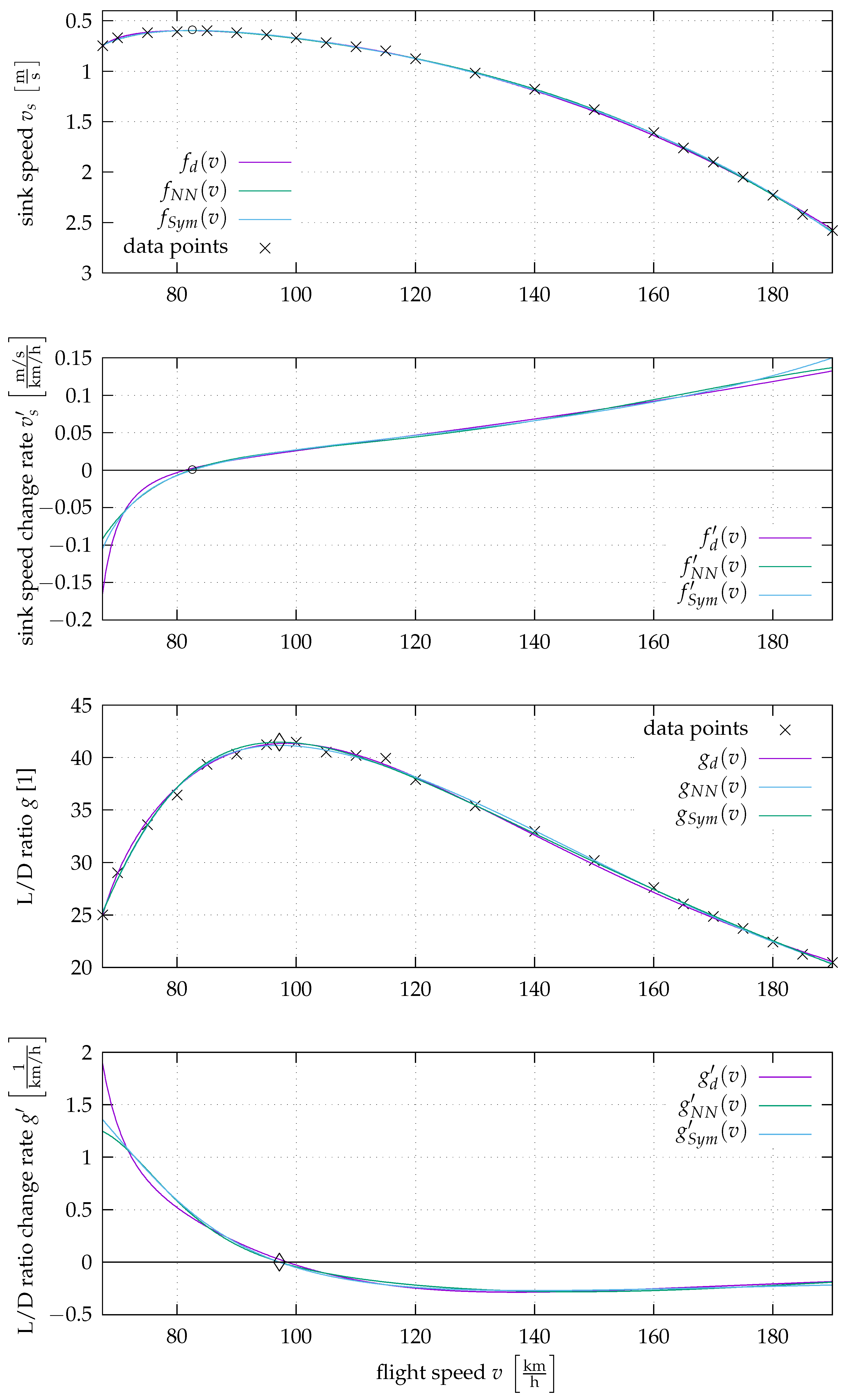
The result values are shown in
Figure 2. The data points are marked by black crosses (×) and the models, as well as their derivatives, in violet for
, in green for
, and in blue for
. In the top diagram, the rate of descent is plotted against the airspeed. This is the typical representation for an aircraft polar. In the second top diagram, the rate of change of the sink rate is plotted against the airspeed. The third diagram from above shows the glide ratio and the bottom diagram shows the rate of change of the glide ratio over the airspeed. This illustration makes it easy to visually understand the relationship between sink rate, glide ratio, and airspeed. In addition, the extreme points can be identified by visualising the derivatives.
The relative error for the sink speeds are given compared to the average of the available sink speed data with a value of . The error calculation was performed using the whole dataset as test points. As only a few data points are available, splitting them into training and test data sets would result in the model only being evaluated based on a handful of points. As a result, models that approximate these few points well are rated well, even if they are only mediocre at representing the data in large parts and vice versa. For this reason, this point was not investigated in more detail and all available data points are used for learning and testing.
3.2.1. Formula Based on Derivation
The physically motivated Formula (
2) was created by Wandinger [
32] using domain knowledge. The derivation is shown in
Appendix A.1. The pole speed
p was manually set to
, which is below the minimal speed. As the parameters
w are always a multiplication factor, the dimensional correctness can be achieved by their appropriate dimensions. The values of the coefficients are
and
.
The root-mean-square error is ~
, which corresponds to 1%, and the maximum error is ~
, which corresponds to 2.5%.
3.2.2. Machine Learning Models
For the machine learning models, the data were scaled to ensure dimensional correctness. This was achieved by correlating the values to the respective maximal values of the data set.
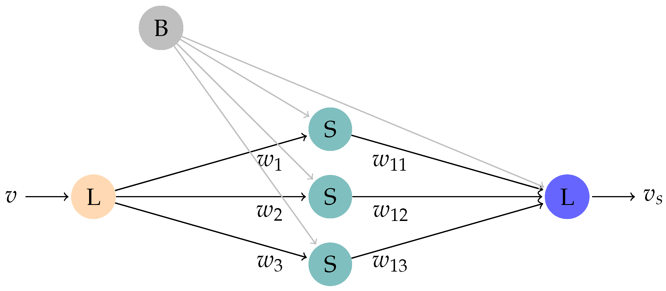
Neural Network Approach. A very simple neural network was created, which is shown in
Figure 3. The formula which represents the network is shown in Equation (
6). For the creation of the neural network, consisting of a single hidden layer with sigmoid activation functions and linear functions in the input and output layers, the package
nnet [
35] was used.
The values of the coefficients are
,
,
,
,
,
,
,
,
and
.
The root-mean-square error is ~
, corresponding to 0.7%, and the maximum error is ~
, corresponding to 1.3%.
Formula by Symbolic Regression. A compact formula, where the variable v occurs only once, was found. The coefficients are and .
The root-mean-square error is ~
, corresponding to 0.8%, and the maximum error is ~
, corresponding to 1.7%.
3.3. Model Validation with Behaviour Envelope
An example of the validation is shown for Formula (
8) found by symbolic regression. Formula (
8) has been preferred over the alternative Formulae (
2) and (
6) for the following reasons: First of all, it is a very compact formula, and secondly, the variable
v occurs in it only once. For
(Formula (
8)), the root-mean-square error is
, corresponding to
, with a maximum error of
, corresponding to
, which leads to the proposition that the data points are well approximated, as the maximum error is only twice as high as the root-mean-squared error. From this, it can be concluded that there are no outliers that are poorly approximated. Nevertheless, the behaviour envelope defined in
Section 3.1 could be used to validate the models
and
in the same way. In
Section 3.1, the expected behaviour envelope was defined, which can be checked step by step:
- 1.
Only interpolation between given data points, as an extrapolation is expected to be unreliable due to the non-linear behaviour of the aircraft aerodynamics (especially at low speeds because of the stall).
The model is limited to the interval .
- 2.
The polar is continuous.
The numerator of the fraction in Equation (
8) is a number and therefore continuous. The denominator is also continuous as it consists of a trigonometric function witch is continuous ([
20] (p. 76)) and a fixed value which is just added. Therefore, it only needs to be ensured that the formula has no pole in the given interval, which is the case when the denominator is as follows:
By transforming the equation, one obtains
In Equation (
11), this is
not fulfilled if
where the value has been rounded to seven decimal places for convenience. Taking the limited interval of
into account, based on Equation (
11),
x can only assume the values in the interval
. (The values were rounded to three decimal places so that the next lower number was used for the lower interval limit and the next higher number for the upper interval limit. This ensures that the interval in question is covered.) Using this, Equation (
12) cannot be fulfilled. (
,
,
,
. As Equation (
12) is a linear equation, this means that for
, no value for
can be achieved.) Based on this, it can be concluded that the found formula has no pole in the given interval and is therefore continuous.
- 3.
The polar contains only one extremum (a minimum), which is at the speed of the best rate of descent.
Extrema can be found by calculating
.
Only
is of interest, as
is out of the allowed interval. If
, it is a minimum:
Therefore, this part of the envelope is fulfilled and
. In
Figure 2, the minimum is marked by a black circle (∘).
- 4.
For the best rate of descent, must be valid. - 5.
The polar has no saddle point.
As has only two solutions where is not in the interval and , the polar has no saddle point.
- 6.
The polar has no turning points, i.e., it is not superimposed by high-frequency oscillations.
As the variable v only occurs within the only trigonometric function, and there is only one extremum in the interval , the model is not able to represent additional oscillations.
- 7.
The best L/D ratio is above 25 (Schleicher K 8, timber construction with covering) and below 70 (eta, best sailplane today).
In the first step, the possible extrema of
need to be found by calculating
:
As it is searched for the best L/D-ratio this has to be a maximum, which means
has a conversion:
As the conversion from positive to negative occurs,
has a maximum at
, which leads to the conclusion
. The best L/D ratio can be calculated as follows:
The L/D ratio
is in the expected interval of
. In
Figure 2, the maximum is marked by a black rhombus (◊).
- 8.
The speed for the best L/D ratio is above the speed for the best rate of descent .
As , this is fulfilled.
As all points are fulfilled, it can be assumed that the model stays in the behaviour envelope. Based on this and the small approximation error, it can be safely assumed that the model is valid.
4. Summary
In order to certify a model for a safety-critical application, it must be ensured that the model is correct. This is a particular challenge for machine learning models, as only a limited number of measurement points are available in real-world applications. However, it must not only be ensured that the model response at the test points has a sufficiently small error for the planned application, but it must also be ensured that the behaviour between the measurement points is correctly mapped. Various approaches have been presented in the past, but due to the complexity (both the reachability problem and the training of a neural network, for example, can be regarded as at least NP-hard), it is unlikely that a method for a complete evaluation with a reasonable runtime will be found in the future. A new approach has therefore been developed that is based on how an expert creates a model based on data. Supplementary to the data set, it is proposed to take the expected behaviour of the system for which the model is designed into account. This is achieved by defining a specific so-called “behaviour envelope”, which defines the area the model is expected to stay within. This requires domain knowledge, whereby, depending on the application, estimates are also sufficient, which can also be fully documented for later evaluation. It can then be mathematically evaluated whether the model remains within the behaviour envelope. This ensures that the behaviour between the test points is reasonable. Since the effort required for the evaluation increases with the complexity of the model, it is suggested to use symbolic regression instead of, for example, neural networks, which means that the effort is shifted more to the creation of the model in order to simplify the validation. The presented approach is shown in an example by modelling the polar of a sailplane.
The key advantage of the “behaviour envelope” is the fact that it represents knowledge about a complex physical system based on fundamental assumptions or other a priori domain knowledge. In the given example, this knowledge is based on fundamental assumptions of flight physics (see
Section 3.1 for the derivation of flight physics considerations). As such, the “behaviour envelope” represents an additional check every potentially physical meaningful model needs to comply to. In consequence, the “behaviour envelope” can be used to check the model statements independent of the generation technique used to establish the model. With human-expert-designed models, a human ensures at every step that the individual terms and their interactions make sense. If a model with symbolic regression is found, it must be subsequently ensured that the model is meaningful (on the one hand, that the test points are hit with a sufficiently small error and, on the other hand, that the behaviour between the test points is meaningful), as this cannot already be achieved during model creation. The methodology presented in this paper was developed for this purpose.
5. Prospect
In this methodology study, our approach is motivated and compared to state-of-the-art machine learning validation approaches. It is demonstrated using a simple example so that the complexity of the models is not too high and does not cause confusion. Nevertheless, for the large aircraft mentioned in the introduction, much more complicated models can be expected. As a result of this, the next step in the development of this approach could be the application of a more extensive system to evaluate the effort for the definition of the behaviour envelope as well as for the mathematical evaluation of the model. Possibilities for automating the evaluation could also be investigated. For a more complicated model, more data points are necessary. As hundreds of thousands of simulations and thousands of hours of test flights are conducted in the aviation industry, many data points could be available, depending on the specific application.
Author Contributions
Conceptualization, M.N., M.A. and S.R.; methodology, M.N., M.A. and S.R.; software, M.N. and M.A.; validation, M.N., M.A. and S.R.; formal analysis, M.N., M.A. and S.R.; investigation, M.N., M.A. and S.R.; data curation, M.N. and M.A.; writing—original draft preparation, M.N., M.A. and S.R.; writing—review and editing, M.N., M.A. and S.R.; visualization, M.N.; supervision, S.R.; project administration, S.R.; funding acquisition, S.R. All authors have read and agreed to the published version of the manuscript.
Funding
This work was supported by the Federal Ministry for Economic Affairs and Climate Action as part of the project “Künstliche Intelligenz Europäisch Zertifizieren unter Industrie 4.0” (KIEZ4-0).
Data Availability Statement
Acknowledgments
The authors would like to thank the Ingenieurgesellschaft für Intelligente Lösungen und Systeme mbH, Trochtelfingen, Germany, (
https://www.iils.de, accessed on 1 May 2025) for the cooperation in the framework of the project KIEZ4-0.
Conflicts of Interest
The authors declare no conflicts of interest. The funders had no role in the design of the study; in the collection, analyses, or interpretation of data; in the writing of the manuscript; or in the decision to publish the results.
Appendix A
Appendix A.1. Derivation of Equation (2)
This section is a summary of Wandinger [
32], which includes the derivation of Equation (
2).
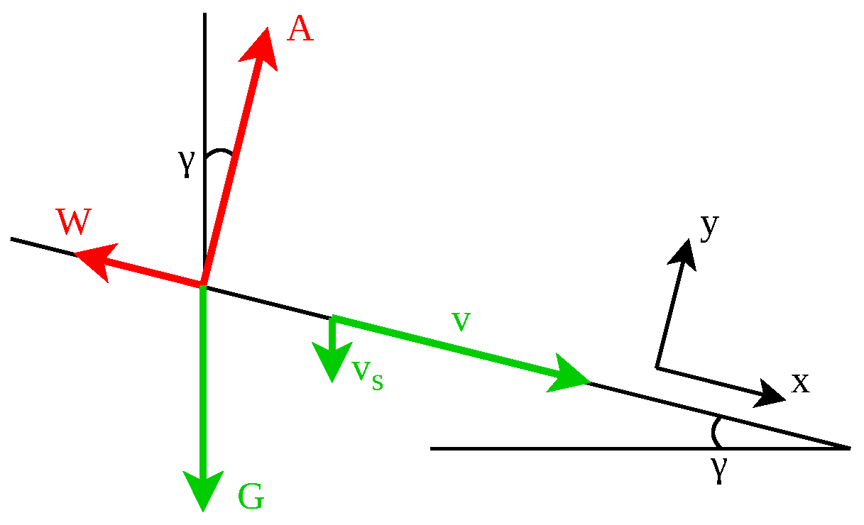
Figure A1.
Stationary flight (based on [
32]).
Figure A1.
Stationary flight (based on [
32]).
In stationary flight, the following follows from the equilibrium of forces
and
where
G is the weight force,
the glide angle,
the mass density of the air,
the drag coefficient,
the lift coefficient and
S the reference surface.
From Equation (A2) follows
Figure A1 shows
Since the glide angle
is small,
as well as
, which leads to
and
With the reference speed
Equation (A7) can be written dimensionless:
The dimensionless velocities
and
were introduced. The dimensionless form of Equation (A6) is
The drag is made up of the form drag and the induced drag. With the form drag coefficient
and a constant
k that depends on the geometry of the wing, the following applies
Substituting Equations (A10) and (A11) into Equation (A9) gives
A high lift coefficient is necessary at low airspeeds. This causes the drag coefficient to rise sharply. To capture this increase, the following approach is used for the drag coefficient
with the constants
,
and the pole
. Using
and
leads to
Substituting Equation (A16) into Equation (A11) and then into Equation (A9) gives
This leads to the tripartite approach
and Equation (
2)
The pole speeds
and
p are manually specified. They must be below the minimum speed. The coefficients
to
or
to
are determined by solving an equalisation problem.
Appendix A.2. Polynomial Model for a Sailplane Polar
The coefficients for the polynomial model are
,
,
,
,
and
.
The root-mean-square error is ~
, corresponding to 1.6%, and the maximum
error is ~
corresponding to 0.8%.
Appendix B
Appendix B.1. Impact of the Model Complexity on the Necessary Validation Effort
Model complexity has a major influence on the effort required for model validation, especially if the derivations are required for this. This is the case, for example, when determining saddle points, extreme points and inflection points. The second derivative and the third derivative are particularly necessary for determining inflection points. In
Section 3.3, point 6 should demonstrate that the model does not contain any inflection points. For
, this could be decided directly due to the simple structure (the model contains only one trigonometric function and is therefore not able to to represent additional oscillations). A calculated proof would be required for
or
, for which the second and third derivatives must be determined:
As the next step, all
for which
and
apply have to be calculated. If there are any, it has to be checked, if
and
, which would mean that the respective
is a inflection point. All this is necessary to ensure that the model is not overlaid by high-frequency oscillations. The fact that such a simple model was found with symbolic regression (Equation (
8)), in which it is easy to see that no superimposition with high-frequency oscillations can occur, has successfully shown that the greater effort in modelling is worthwhile, as this can reduce the effort required for validation.
References
- EASA. Certification Specifications and Acceptable Means of Compliance for Large Aeroplanes (CS-25) 2021. Amendment 27. Available online: https://www.easa.europa.eu/en/document-library/certification-specifications/cs-25-amendment-27 (accessed on 4 February 2025).
- EASA. EASA Concept Paper: First Usable Guidance for Level 1 & 2 Machine Learning Applications 2023. Available online: https://www.easa.europa.eu/en/downloads/137631/en (accessed on 4 February 2025).
- Notter, S.; Schimpf, F.; Fichter, W. Hierarchical Reinforcement Learning Approach Towards Autonomous Cross-Country Soaring. In AIAA Scitech 2021 Forum; ARC: Gillingham, Kent, 2021. [Google Scholar] [CrossRef]
- Lam, R.; Sanchez-Gonzalez, A.; Willson, M.; Wirnsberger, P.; Fortunato, M.; Alet, F.; Ravuri, S.; Ewalds, T.; Eaton-Rosen, Z.; Hu, W.; et al. Learning skillful medium-range global weather forecasting. Science 2023, 382, 1416–1421. [Google Scholar] [CrossRef] [PubMed]
- Wartha, N.; Stephan, A.; Holzäpfel, F.; Rotshteyn, G. Characterizing aircraft wake vortex position and strength using LiDAR measurements processed with artificial neural networks. Opt. Express 2022, 30, 13197–13225. [Google Scholar] [CrossRef] [PubMed]
- Cortes, C.; Jackel, L.D.; Chiang, W.P. Limits on Learning Machine Accuracy Imposed by Data Quality. In Proceedings of the Advances in Neural Information Processing Systems, Denver, CO, USA, 28 November–1 December 1994; Tesauro, G., Touretzky, D., Leen, T., Eds.; MIT Press: Cambridge, MA, USA, 1994; Volume 7. [Google Scholar]
- Budach, L.; Feuerpfeil, M.; Ihde, N.; Nathansen, A.; Noack, N.; Patzlaff, H.; Naumann, F.; Harmouch, H. The Effects of Data Quality on Machine Learning Performance. arXiv 2022, arXiv:2207.14529. [Google Scholar]
- Botchkarev, A. A New Typology Design of Performance Metrics to Measure Errors in Machine Learning Regression Algorithms. Interdiscip. J. Inf. Knowl. Manag. 2019, 14, 045–076. [Google Scholar] [CrossRef] [PubMed]
- Gawlikowski, J.; Tassi, C.R.N.; Ali, M.; Lee, J.; Humt, M.; Feng, J.; Kruspe, A.; Triebel, R.; Jung, P.; Roscher, R.; et al. A survey of uncertainty in deep neural networks. Artif. Intell. Rev. 2023, 56, 1513–1589. [Google Scholar] [CrossRef]
- Liu, C.; Arnon, T.; Lazarus, C.; Strong, C.; Barrett, C.; Kochenderfer, M.J. Algorithms for Verifying Deep Neural Networks. Found. Trends Optim. 2021, 4, 244–404. [Google Scholar] [CrossRef]
- Carvalho, D.V.; Pereira, E.M.; Cardoso, J.S. Machine Learning Interpretability: A Survey on Methods and Metrics. Electronics 2019, 8, 832. [Google Scholar] [CrossRef]
- Tambon, F.; Laberge, G.; An, L.; Nikanjam, A.; Mindom, P.S.N.; Pequignot, Y.; Khomh, F.; Antoniol, G.; Merlo, E.; Laviolette, F. How to certify machine learning based safety-critical systems? A systematic literature review. Autom. Softw. Eng. 2022, 29, 38. [Google Scholar] [CrossRef]
- Sälzer, M.; Lange, M. Reachability is NP-Complete Even for the Simplest Neural Networks. In Proceedings of the Reachability Problems, Liverpool, UK, 25–27 October 2021; Bell, P.C., Totzke, P., Potapov, I., Eds.; Springer: Cham, Switzerland, 2021; pp. 149–164. [Google Scholar] [CrossRef]
- Wurm, A. Complexity of Reachability Problems in Neural Networks. In Proceedings of the Reachability Problems, Nice, France, 11–13 October 2023; Bournez, O., Formenti, E., Potapov, I., Eds.; Springer: Cham, Switzerland, 2023; pp. 15–27. [Google Scholar] [CrossRef]
- Katz, G.; Barrett, C.; Dill, D.L.; Julian, K.; Kochenderfer, M.J. Reluplex: An Efficient SMT Solver for Verifying Deep Neural Networks. In Proceedings of the Computer Aided Verification, Heidelberg, Germany, 24–28 July 2017; Majumdar, R., Kunčak, V., Eds.; Springer: Cham, Switzerland, 2017; pp. 97–117. [Google Scholar] [CrossRef]
- Sälzer, M.; Lange, M. Fundamental Limits in Formal Verification of Message-Passing Neural Networks. arXiv 2022, arXiv:2206.05070. [Google Scholar]
- Jones, L. The computational intractability of training sigmoidal neural networks. IEEE Trans. Inf. Theory 1997, 43, 167–173. [Google Scholar] [CrossRef]
- Abrahamsen, M.; Kleist, L.; Miltzow, T. Training Neural Networks is ER-complete. In Proceedings of the Advances in Neural Information Processing Systems, Online, 6–14 December 2021; Ranzato, M., Beygelzimer, A., Dauphin, Y., Liang, P., Vaughan, J.W., Eds.; Curran Associates, Inc.: Red Hook, NY, USA, 2021; Volume 34, pp. 18293–18306. [Google Scholar]
- D’Amour, A.; Heller, K.; Moldovan, D.; Adlam, B.; Alipanahi, B.; Beutel, A.; Chen, C.; Deaton, J.; Eisenstein, J.; Hoffman, M.D.; et al. Underspecification presents challenges for credibility in modern machine learning. J. Mach. Learn. Res. 2022, 23, 10237–10297. [Google Scholar]
- Bronshtein, I.; Semendyayev, K.; Musiol, G.; Mühlig, H. Handbook of Mathematics, 6th ed.; Springer: Berlin/Heidelberg, Germany, 2015. [Google Scholar] [CrossRef]
- Walz, G. (Ed.) Lexikon der Mathematik: Band 2; Springer: Berlin/Heidelberg, Germany, 2017. [Google Scholar] [CrossRef]
- Schmidt, M.; Lipson, H. Distilling Free-Form Natural Laws from Experimental Data. Science 2009, 324, 81–85. [Google Scholar] [CrossRef] [PubMed]
- Udrescu, S.M.; Tegmark, M. AI Feynman: A physics-inspired method for symbolic regression. Sci. Adv. 2020, 6, eaay2631. [Google Scholar] [CrossRef] [PubMed]
- Anselment, M.; Neumaier, M.; Rudolph, S. Von Daten zu physikalischen Modellen mit Methoden der Künstlichen Intelligenz. In Proceedings of the Deutscher Luft- und Raumfahrtkongress, Stuttgart, Germany, 19–21 September 2023. [Google Scholar]
- Anselment, M.; Neumaier, M.; Rudolph, S. Symbolic Regression: Systematically Spanning and Searching the Space of Dimensionally Homogeneous Symbolic Models using a Tree Search. CEAS Aeronaut. J. 2025; submitted. [Google Scholar]
- Virgolin, M.; Pissis, S.P. Symbolic Regression is NP-hard. arXiv 2022, arXiv:2207.01018. [Google Scholar]
- Keren, L.S.; Liberzon, A.; Lazebnik, T. A computational framework for physics-informed symbolic regression with straightforward integration of domain knowledge. Sci. Rep. 2023, 13, 1249. [Google Scholar] [CrossRef] [PubMed]
- Laplante, P.A.; Kassab, M.H. Requirements Engineering for Software and Systems; Auerbach Publications: Boca Raton, FL, USA, 2022. [Google Scholar] [CrossRef]
- Simon, V.; Weigand, B.; Gomaa, H. Dimensional Analysis for Engineers; Springer: Cham, Switzerland, 2017. [Google Scholar] [CrossRef]
- Görtler, H. Dimensionsanalyse; Ingenieurwissenschaftliche Bibliothek; Springer: Berlin/Heidelberg, Germany, 1975. [Google Scholar]
- Schempp-Hirth Flugzeug-Vertriebs GmbH. Flugzeuge von Klaus Holighaus (1964–1994). 2025. Available online: https://www.schempp-hirth.com/unternehmen/historie/flugzeuge-von-klaus-holighaus-1964-1994 (accessed on 24 January 2025).
- Wandinger, J. Ein einfacher Approximationsansatz für die Geschwindigkeitspolare eines Segelflugzeugs. 2011. Available online: https://www.researchgate.net/publication/378631423_Ein_einfacher_Approximationsansatz_fur_die_Geschwindigkeitspolare_eines_Segelflugzeugs?channel=doi&linkId=65e1d854e7670d36abe8956f&showFulltext=true (accessed on 4 February 2025).
- Alexander Schleicher GmbH. K 8/K 8 B/K 8 C. 2025. Available online: https://www.alexander-schleicher.de/en/flugzeuge/k-8-k-8-b-k-8-c/ (accessed on 24 January 2025).
- Flugtechnik und Leichtbau. Leistungsvermessung. 2025. Available online: https://www.leichtwerk.de/eta-aircraft/de/flugerprobung/leistung.html (accessed on 24 January 2025).
- Venables, W.N.; Ripley, B.D. Modern Applied Statistics with S, 4th ed.; Springer: New York, NY, USA, 2002; ISBN 0-387-95457-0. [Google Scholar]
| Disclaimer/Publisher’s Note: The statements, opinions and data contained in all publications are solely those of the individual author(s) and contributor(s) and not of MDPI and/or the editor(s). MDPI and/or the editor(s) disclaim responsibility for any injury to people or property resulting from any ideas, methods, instructions or products referred to in the content. |
© 2025 by the authors. Licensee MDPI, Basel, Switzerland. This article is an open access article distributed under the terms and conditions of the Creative Commons Attribution (CC BY) license (https://creativecommons.org/licenses/by/4.0/).


