Multi-Point Optimization Design of Blended Wing Body Based on Discrete Adjoint Method

Abstract

In actual flight, aircraft rarely operate under a single design condition; multiple flight states must be considered to meet performance requirements. With the push for green and low-carbon aviation, there is growing demand for high-performance, fuel-efficient aircraft. This study focuses on the Blended Wing Body (BWB) configuration. To address large-scale design variables and multiple constraints, a discrete adjoint-based aerodynamic optimization method is developed, improving computational efficiency and reducing cost.The optimization results show reduced drag coefficients across various flight conditions and enhanced drag divergence performance. The robustness of the multi-point optimization approach is validated, confirming its ability to improve aircraft performance across different states. The proposed method is practical and provides an effective reference for aerodynamic design of BWB aircraft.

1. Introduction

With the ongoing economic prosperity and the rapid development of the aviation industry, increasing environmental concerns and fuel consumption issues have posed new challenges for the design of next-generation aircraft. To meet the demands of market development and achieve the goal of “Green Aviation”, conventional aircraft configurations are no longer sufficient. The Blended Wing Body (BWB) aircraft has emerged as a promising alternative due to its lightweight structure, high aerodynamic efficiency, and reduced fuel consumption [1,2,3].

Despite these advantages, the development of BWB aircraft still faces numerous technical challenges, among which aerodynamic shape optimization plays a critical role. Optimization methods can generally be categorized into two types: global optimization algorithms and gradient-based algorithms. Global optimization methods offer strong adaptability and global search capabilities but are computationally expensive. Gradient-based methods, on the other hand, provide efficient local search and faster convergence but often struggle to accurately and efficiently compute the gradient of the objective function with respect to a large number of design variables. This issue becomes particularly prominent in high-dimensional optimization problems. To address this challenge, Antony Jameson [4] introduced the adjoint method into the field of aeronautical design, significantly reducing computational cost and improving optimization efficiency.

Subsequent research has demonstrated the effectiveness of adjoint-based methods in aerodynamic shape optimization. For instance, He et al. [5] implemented the discrete adjoint method using OpenFOAM for aerodynamic design. Jeffrey et al. [6] conducted nonlinear unsteady optimization based on adjoint formulations. Abergo et al. [7] employed radial basis function (RBF) mesh deformation in combination with a discrete adjoint method for wing drag reduction. Ma et al. [8] proposed an optimization strategy based on equivalent area distribution using a discrete adjoint approach. Belda et al. [9] combined adjoint and parametric methods for interactive airfoil optimization. In China, Liu et al. [10] applied the Navier–Stokes equations with an adjoint method to optimize transonic drag reduction for wings with varying aspect ratios. Lei et al. [11] explored serial and parallel optimization of flying wing aircraft using a coupled aerodynamic/structural adjoint method. Zhang et al. [12] developed an aerodynamic optimization approach for full aircraft configurations that accounts for dynamic effects. Li et al. [13] established a multidisciplinary gradient-based optimization system for aerodynamic stealth design of UAVs. Wang et al. [14] developed both steady and unsteady airfoil optimization methods based on the discrete adjoint approach.

Although these studies have produced mature results in adjoint-based aerodynamic optimization, most focus on single-point optimization or simplified configurations. A significant research gap remains in the area of multi-point aerodynamic optimization for BWB configurations [15,16]. Key challenges include managing large numbers of design variables, satisfying complex nonlinear constraints, and ensuring computational efficiency across multiple flight conditions. Moreover, achieving accurate CFD simulations over a range of flight states adds further complexity—particularly in resolving aerodynamic sensitivities and maintaining convergence consistency across the design space.

In summary, substantial progress has been made in adjoint-based aerodynamic optimization, offering a solid foundation for further research. However, there remains considerable potential for development, particularly in the context of multi-point optimization for BWB aircraft.

To address this, the present study constructs an aerodynamic shape optimization framework based on the discrete adjoint method, utilizing the open-source SU2 platform developed by Stanford University [17]. The framework integrates CFD flow field solvers with a three-dimensional Free-Form Deformation (FFD) parameterization method, elastomeric mesh deformation, and an SLSQP optimization algorithm.

2. Simulation Method

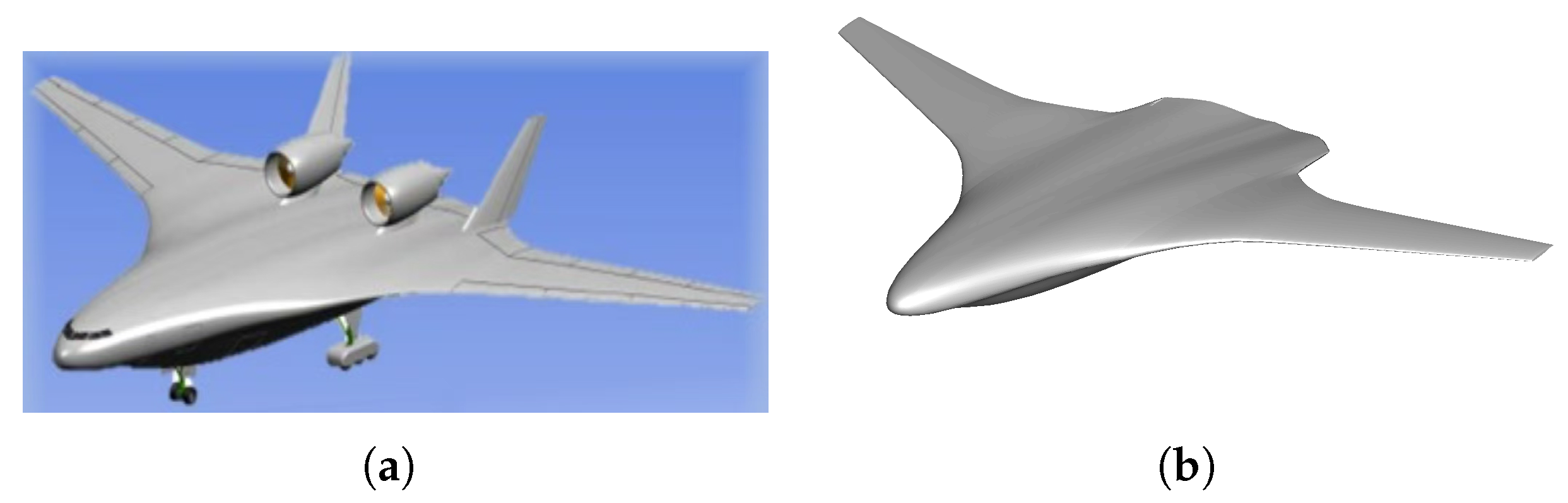
2.1. Wing Model

The subject of this study is the N2A aircraft, a Hybrid Wing Body (HWB) civil transport concept proposed by NASA under the ERA “N+2” project, aiming to reduce noise and fuel consumption [18]. The aircraft model used in this work is illustrated in Figure 1.

The N2A configuration was selected due to its relevance to next-generation commercial aviation objectives, particularly those targeting environmental sustainability. As part of NASA’s environmentally responsible aviation (ERA) initiative, the N2A model aims to achieve significant reductions in community noise, fuel burn, and emissions, making it a representative and valuable case for aerodynamic optimization research.

The baseline configuration features a blended wing-fuselage design with distributed thickness and smooth curvature transitions, ideal for evaluating aerodynamic performance across various flight regimes. This study incorporates three design conditions—low-speed, subsonic, and transonic—characterized by Mach numbers of 0.2, 0.4, and 0.7, and corresponding Reynolds numbers of $6.6\times {10}^6$, $9.5\times {10}^6$, and $1.6\times {10}^7$, respectively. The angles of attack for each state are set based on trim conditions to maintain constant lift. These representative conditions were selected to capture a broad portion of the flight envelope, providing a robust testbed for multi-point optimization.

2.2. Numerical Methodologies

The flow field is governed by the Reynolds-Averaged Navier–Stokes (RANS) equations, with the Shear Stress Transport (SST) turbulence model adopted [19]. These equations are discretized spatially using a cell-centered finite volume method. The viscous terms are treated with a second-order central difference scheme, while inviscid terms are computed using the second-order upwind JST scheme [20]. Time integration is performed using the implicit Euler method. Multi-level grids are employed to accelerate convergence.

A structured grid is generated using Gmsh 4.0.4, a widely used open-source mesh generation software, ensuring $Y^{+}\approx 1$. Local mesh refinement is applied near the leading and trailing edges of the wing, as well as in the wall-normal direction near the body surface. The grid configuration is shown in Figure 2.

The aerodynamic force coefficients are calculated as follows:

$$C_L={\displaystyle \frac{L}{\frac{1}{2}{\rho }_{\infty }{V}_{\infty }^2{S}_{ref}}},C_D={\displaystyle \frac{D}{\frac{1}{2}{\rho }_{\infty }{V}_{\infty }^2{S}_{ref}}},C_M={\displaystyle \frac{M}{\frac{1}{2}{\rho }_{\infty }{V}_{\infty }^2{S}_{ref}}},C_P={\displaystyle \frac{p-p_{\infty }}{\frac{1}{2}{\rho }_{\infty }{V}_{\infty }^2}}$$

(1)

where L is the lift force, D is the drag force, M is the pitching moment, p is the surface pressure, $p_{\infty }$ is the free-stream pressure, ${\rho }_{\infty }$ is the free-stream fluid density, $V_{\infty }$ is the free-stream velocity, and $S_{ref}$ is the reference area.

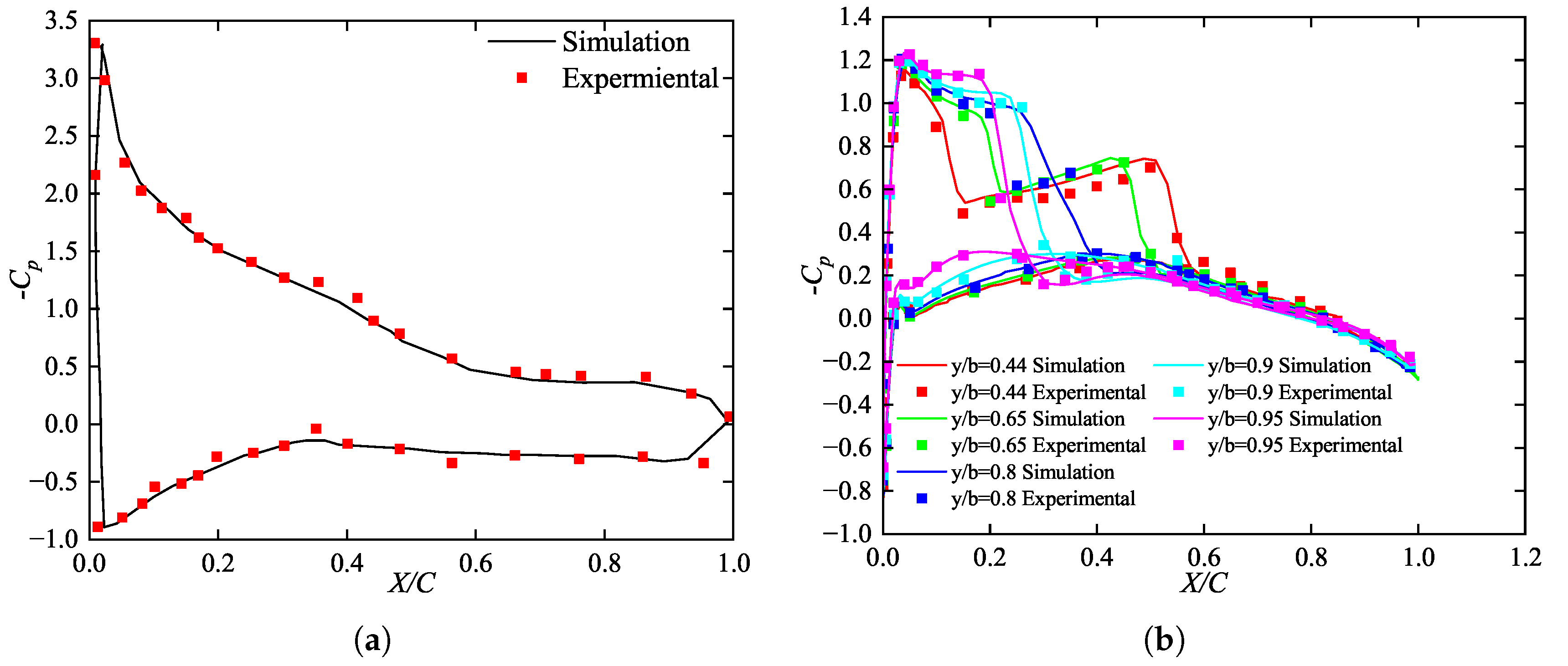
2.3. Solver Validation

To verify the accuracy and reliability of the numerical method, two validation cases are considered: the NREL S826 airfoil for low-speed flow and the ONERA M6 wing for transonic conditions.

Case 1: NREL S826 airfoil. Design conditions are: $Ma=0.19$, $Re=1\times {10}^5$, $\alpha =8^{\circ }$ [21]. A C-type structured mesh is used, with $Y^{+}\approx 1$ and refinement at the leading and trailing edges. The computed pressure coefficient ($C_P$) distribution is compared with experimental data in Figure 3a.

Case 2: ONERA M6 wing. Design conditions are: $Ma=0.8395$, $Re=11.72\times {10}^6$, $\alpha =3.{06}^{\circ }$ [22]. An O-H structured grid is employed with $Y^{+}\approx 1$, and local refinement around the leading/trailing edges and fuselage surfaces. The computed $C_P$ distribution is compared with experimental results in Figure 3b, using data from [23,24].

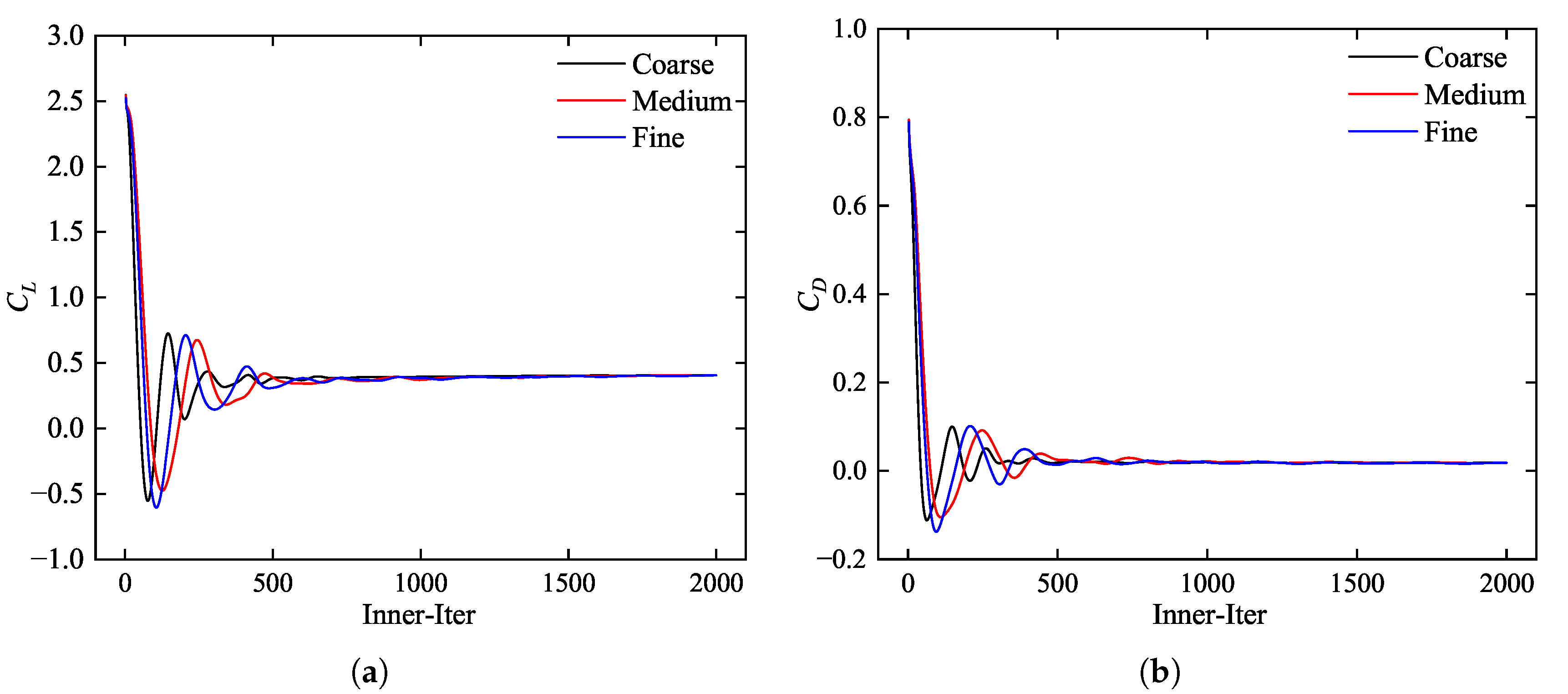
2.4. Mesh Independence Study

To verify the independence of the grid results, three mesh sizes were tested: $0.6\times {10}^6$, $1.19\times {10}^6$, and $2.59\times {10}^6$ elements. The simulations were conducted under the design state conditions: Ma = 0.2, Re = $6.6\times {10}^6$, and $\alpha =8.{36}^{\circ }$. The results of the aerodynamic coefficients are presented in Figure 4.

3. Optimization Method

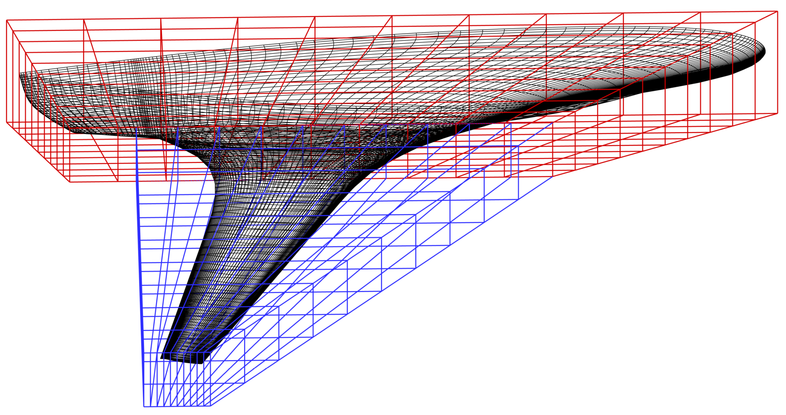
3.1. Parametric Modeling: Free Form Deformation (FFD)

Free Form Deformation (FFD) is a powerful geometric parameterization technique used to manipulate complex shapes. FFD represents the shape of a structure as a lattice of control points, which can be moved to deform the shape in a smooth and continuous manner. Mathematically, FFD is based on a tensor product of Bézier curves, which enables smooth and flexible shape modifications without introducing discontinuities. This method provides an efficient way to parameterize 3D surfaces and volumes, making it highly suitable for aerodynamic shape optimization.Compared to traditional parameterization methods such as NURBS or splines, FFD offers superior flexibility and can easily handle both global and local shape changes. It is particularly useful in aerodynamic optimization, where smooth and continuous deformations are required to improve performance without affecting the structural integrity of the geometry [25].

3.2. Mesh Deformation: Elastomeric Method

The elastomeric method for mesh deformation is based on the analogy of a mesh behaving like a network of springs or elastomers. When a surface perturbation is applied, the mesh nodes are moved, and the deformation is propagated throughout the mesh by solving a system of spring-like equations. This method ensures that the mesh remains of high quality during deformation, which is critical for accurate computational fluid dynamics (CFD) simulations. One of the key advantages of the elastomeric method is its ability to maintain smoothness and avoid mesh distortions, particularly in structured grids where traditional deformation techniques may lead to mesh tangling. This method is well-suited for large deformations, as it ensures the mesh adapts to the new geometry without introducing significant errors in the computational domain. The elastomeric method also guarantees that the mesh quality is preserved, which is crucial for solving the governing flow equations accurately and efficiently.

3.3. Discrete Adjoint Method

The adjoint method can be classified into two types: the continuous adjoint method and the discrete adjoint method. The continuous adjoint method formulates the adjoint problem based on the continuous flow equations [26], while the discrete adjoint method derives the adjoint equations from the discretized form of the governing equations, using the residuals of the discretized system as constraints [27].

Let the objective function be defined as I, which depends on the flow field solution vector $W\left(v\right)$ and the spatial grid $X\left(v\right)$, both parameterized by the design variable v:

$$I=I\left(W\right(v),X(v\left)\right)$$

(2)

When the flow field solution is known, the governing Equation (2) can be represented as:

$$R\left(W\right(v),X(v\left)\right)=0$$

(3)

Taking the total derivative of the objective function with respect to v yields:

$${\displaystyle \frac{dI}{dv}}={\displaystyle \frac{\partial I}{\partial W}}·{\displaystyle \frac{dW}{dv}}+{\displaystyle \frac{\partial I}{\partial X}}·{\displaystyle \frac{dX}{dv}}$$

(4)

Similarly, the total derivative of the residual equations with respect to v is:

$${\displaystyle \frac{dR}{dv}}={\displaystyle \frac{\partial R}{\partial W}}·{\displaystyle \frac{dW}{dv}}+{\displaystyle \frac{\partial R}{\partial X}}·{\displaystyle \frac{dX}{dv}}$$

(5)

Substituting Equation (5) into Equation (4), we obtain:

$${\displaystyle \frac{dI}{dv}}=\left[{\displaystyle \frac{\partial I}{\partial X}}-{\displaystyle \frac{\partial I}{\partial W}}{\left({\displaystyle \frac{\partial R}{\partial W}}\right)}^{-1}{\displaystyle \frac{\partial R}{\partial X}}\right]{\displaystyle \frac{dX}{dv}}$$

(6)

To avoid directly inverting the Jacobian matrix, we introduce the adjoint variable $\Psi$ as:

$${\Psi }^T={\displaystyle \frac{\partial I}{\partial W}}{\left({\displaystyle \frac{\partial R}{\partial W}}\right)}^{-1}$$

(7)

This transforms the matrix inversion into the solution of a linear system:

$${\left({\displaystyle \frac{\partial R}{\partial W}}\right)}^T\Psi ={\left({\displaystyle \frac{\partial I}{\partial W}}\right)}^T$$

(8)

Therefore, Equation (6) becomes:

$${\displaystyle \frac{dI}{dv}}=\left[{\displaystyle \frac{\partial I}{\partial X}}-{\Psi }^T{\displaystyle \frac{\partial R}{\partial X}}\right]{\displaystyle \frac{dX}{dv}}$$

(9)

Here, ${\displaystyle \frac{\partial I}{\partial X}}$ is the sensitivity of the objective function to the grid, ${\displaystyle \frac{\partial R}{\partial X}}$ is the sensitivity of the residual to the grid, and ${\displaystyle \frac{dX}{dv}}$ is the grid sensitivity with respect to the design variables.

This completes the gradient derivation for the discrete adjoint method. Solving the adjoint equation (Equation (9)) is key to computing the gradient.

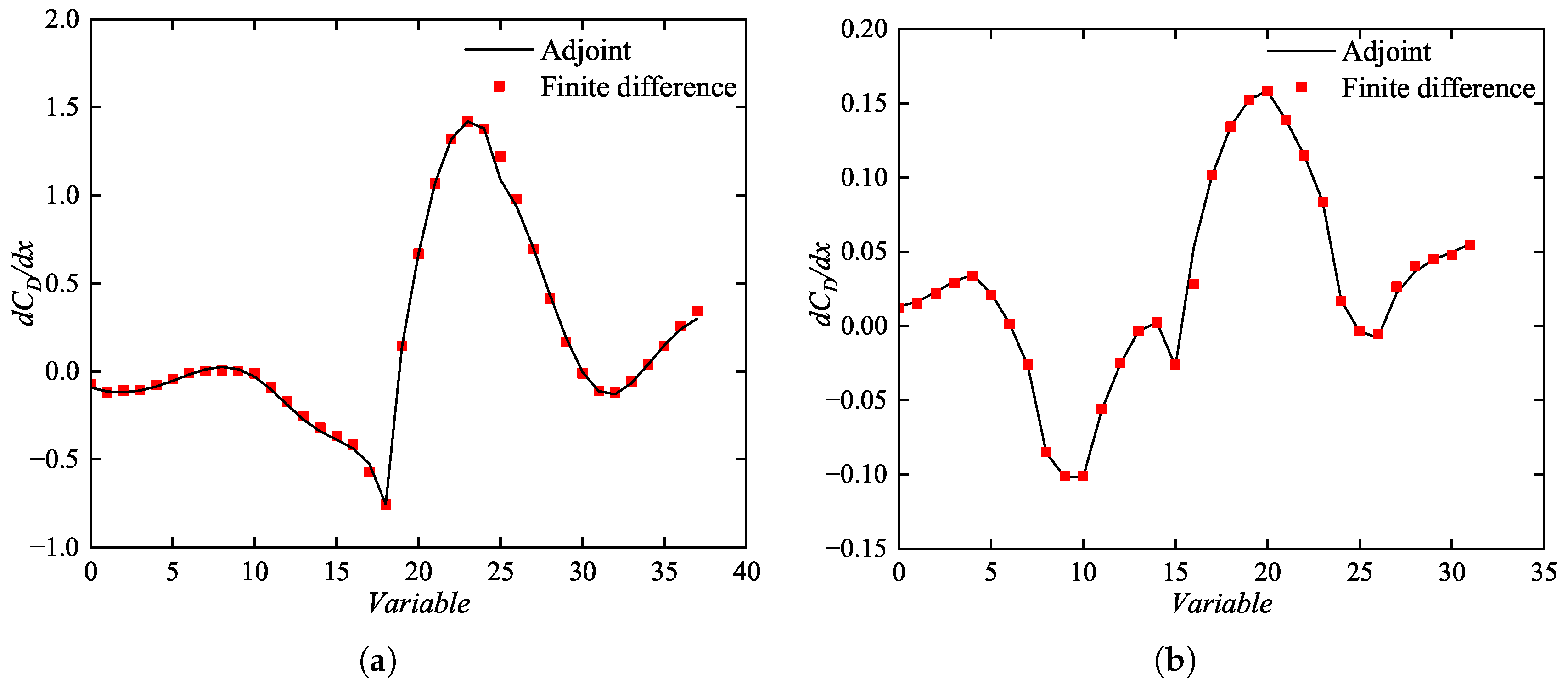
Adjoint Gradient Accuracy Validation

To verify the accuracy and reliability of the discrete adjoint method, gradients computed by the discrete adjoint approach are compared with those obtained using the finite difference method in two test cases. A consistent step size is used for finite difference to ensure fair comparison.

Case 1: RAE 2822 airfoil, design condition [28]: $Ma=0.73$, $Re=6.5\times {10}^6$, $\alpha =2.7^{\circ }$. The Hicks-Henne parameterization method is used, with 38 Hicks-Henne design variables (19 on the upper surface and 19 on the lower surface), distributed along the chord at 5%, 10%, …, 95%. The finite difference step size is $1\times {10}^{-3}$. The sensitivity of the drag coefficient with respect to design variables from both methods is shown in Figure 5a.

Case 2: NACA 0012 airfoil, design condition [29]: $Ma=0.7$, $Re=9\times {10}^6$, $\alpha =1.{55}^{\circ }$. The Hicks-Henne method is also used, with 32 Hicks-Henne design variables (16 for upper and 16 for lower surface), distributed similarly. The finite difference step size is $1\times {10}^{-3}$. The comparison is presented in Figure 5b.

3.4. Optimization Algorithm: Sequential Least Squares Programming (SLSQP)

The optimization process is performed using the Sequential Least Squares Programming (SLSQP) algorithm, a well-established gradient-based method designed to solve nonlinear constrained optimization problems. SLSQP is particularly effective in handling problems with a large number of design variables and constraints, as it combines gradient-based optimization with quadratic programming to handle both equality and inequality constraints. Compared to other optimization methods, such as the Nelder-Mead method or genetic algorithms, SLSQP provides faster convergence and more accurate solutions for problems involving smooth and differentiable objective functions, such as aerodynamic shape optimization. Its robustness and ability to handle large optimization problems make it ideal for aerodynamic shape optimization in real-world engineering applications.

3.5. Computing Platform: SU2 Solver

The simulations are conducted using SU2, an open-source computational fluid dynamics (CFD) solver developed by Stanford University. SU2 is widely used in aerodynamic shape optimization due to its support for adjoint-based optimization, high-fidelity turbulence modeling, and parallel computation capabilities. The primary reasons for choosing SU2 is its open-source nature, which provides transparency and flexibility for users. It supports a wide range of solvers and numerical methods, including those for compressible and incompressible flows, and is validated against experimental benchmarks such as the NREL S826 wind turbine and ONERA M6 wing. The solver’s accuracy in predicting aerodynamic performance is demonstrated through comparisons with experimental data, making it a reliable tool for high-fidelity aerodynamic simulations. Furthermore, SU2’s ability to handle complex geometries and large-scale optimization problems makes it an ideal choice for this study.

4. Aerodynamic Shape Optimization Design

In this paper, two Free Form Deformation (FFD) boxes are employed for parametric modeling, as they provide greater flexibility in deformation and enable more precise shape adjustments for the Blended Wing Body (BWB). The dimensions of the two FFD boxes are set to $10\times 10\times 1$, and the corresponding number of control points is $11\times 11\times 2=242$, totaling 484 control points. The layout of the two boxes is shown in Figure 6, where Box 1 is represented in red and Box 2 in blue. The control points can only move vertically along the fuselage.

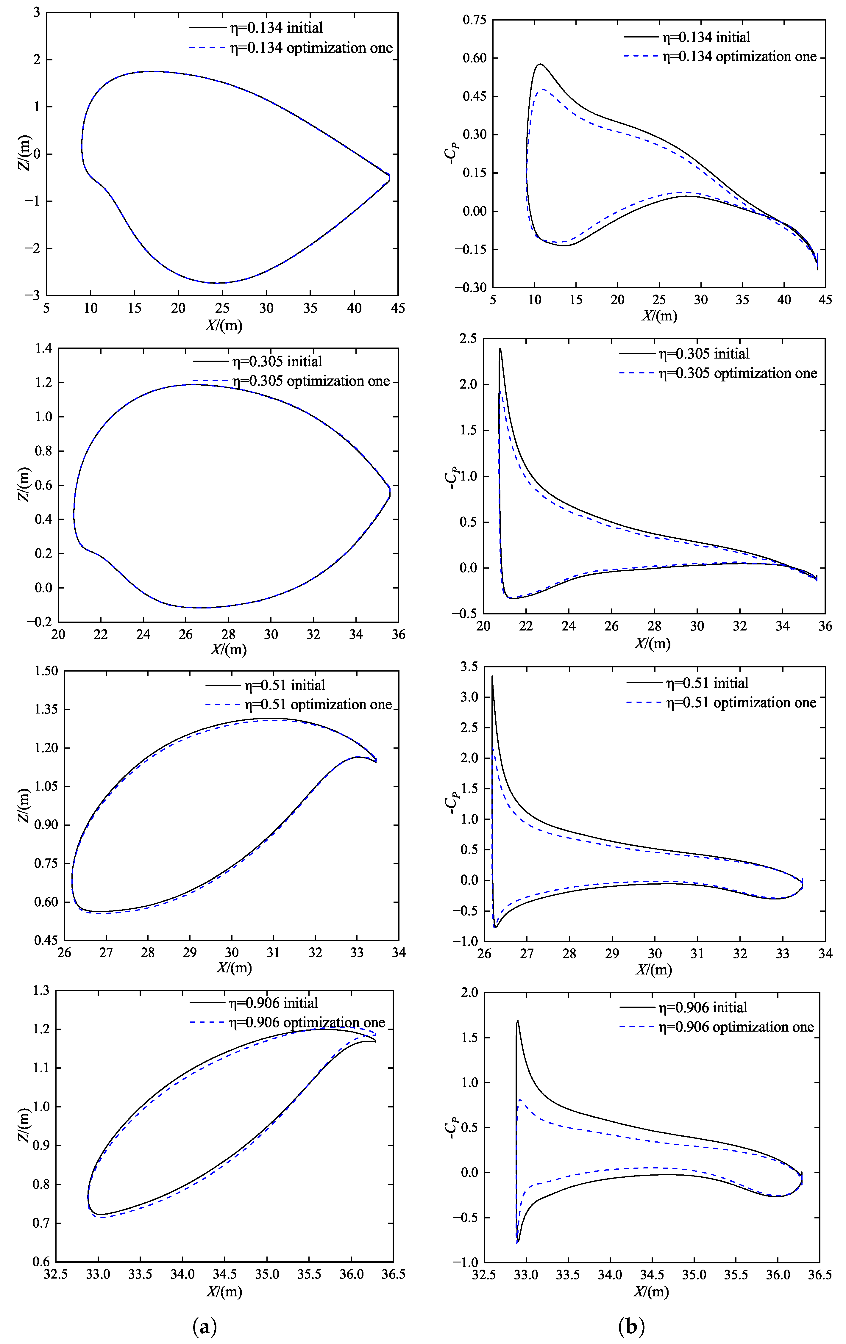
4.1. Optimization Configuration One

The initial design state is as follows: Mach number ($Ma$) = 0.2, Reynolds number ($Re$) = $6.6\times {10}^6$, and angle of attack ($\alpha$) = $8.{36}^{\circ }$ [30]. As shown in

Table 1. Optimization Configuration One: Design States.

Design State	Ma	${\mathit{C}}_{\mathit{L}}$
A	0.1	0.405
B (Cruise)	0.2	0.405
C	0.3	0.405

, three design states near the cruising Mach number are selected.

The objective function for each design state is transformed into a weighted objective function using a weighted sum method. The design variables of the optimization problem include both geometric and aerodynamic variables. The optimization problem is described as:

Objective:

$$minf\left(x\right)=\sum _{i=A,B,C}{W}_i{C}_D$$

Design Variables:

$$Z_{\mathrm{wing}},{\alpha }_i$$

Constraints:

$$C_L=C_{L,\mathrm{init}},\left|C_{M_y,A,B,C}\right|\le C_{M_y,A,\mathrm{init},B,\mathrm{init},C,\mathrm{init}},T_1\ge T_{1,\mathrm{init}},T_2\ge T_{2,\mathrm{init}},T_3\ge T_{3,\mathrm{init}},T_4\ge T_{4,\mathrm{init}}.$$

where $W_i$ is the weight control parameter. Based on relevant domestic literature and textbooks, the weight control parameters for design states A, B, and C are set to 0.25, 0.5, and 0.25, respectively. This indicates that the optimization weight for the cruise state B is higher than that for states A and C.

$Z_{\mathrm{wing}}$ consists of 484 control points. ${\alpha }_i$ is the angle of attack of the incoming flow, with three design variables corresponding to the design states. During aerodynamic optimization, the angle of attack must be adjusted continuously to maintain a constant lift coefficient in order to satisfy the design conditions.

• $C_L$ is the lift coefficient.
• $C_{L,\mathrm{init}}$ is the initial lift coefficient, which ensures the balance between lift and gravity during flight through the constant lift constraint.
• $C_{My}$ is the pitch moment coefficient after optimization.
• $C_{My,\mathrm{init}}$ is the initial pitch moment coefficient.
• $T_1$ and $T_{1,\mathrm{init}}$, $T_2$ and $T_{2,\mathrm{init}}$, $T_3$ and $T_{3,\mathrm{init}}$, $T_4$ and $T_{4,\mathrm{init}}$ represent the optimized and original airfoil thicknesses at four sections ($\eta =y/b=13.4\%$, $30.5\%$, $51\%$, $90.6\%$) along the BWB. These sections’ airfoil thickness should not decrease after optimization.

The optimization process tends to converge by the 8th iteration, as shown in Figure 7. It can be observed that the lift coefficient remains nearly constant, while the drag coefficient decreases for the three design states.

As shown in

Table 2. Aerodynamic Coefficients Comparison for Optimization Configuration One.

Configuration	$\mathit{Ma}$	${\mathit{C}}_{\mathit{L}}$	${\mathit{C}}_{\mathit{D}}$	${\mathit{C}}_{\mathit{L}}/{\mathit{C}}_{\mathit{D}}$	$\sqrt{{\mathit{C}}_{\mathit{L}}}/{\mathit{C}}_{\mathit{D}}$	${\mathit{C}}_{\mathit{My}}$	$\mathit{\alpha }{(}^{\circ })$
Basic Configuration	0.1	0.405	0.0177	22.88	35.95	−0.00854	9.31
	0.2	0.405	0.0184	22.01	34.59	−0.00511	8.36
	0.3	0.405	0.0203	19.95	31.34	−0.00493	7.41
Single-Point Optimization	0.1	0.405	0.0179	22.63	35.57	0.000629	11.76
	0.2	0.405	0.0164	24.70	38.82	−0.000485	10.56
	0.3	0.405	0.0196	20.66	32.45	0.00427	10.26
Multi-Point Optimization	0.1	0.405	0.0172	23.55	37.01	0.00686	12.91
	0.2	0.405	0.0167	24.25	38.10	0.00225	12.11
	0.3	0.405	0.0185	21.89	34.41	−0.00391	11.01

, the basic configurations of the three design states and the aerodynamic coefficients from both single-point and multi-point optimizations are presented.

It can be observed that the pitching moment coefficients for each state meet the constraint conditions. Additionally, the thickness of each section also satisfies the given constraints. In the multi-point optimization configuration, the drag coefficient decreases by 2.82% in the low Mach number state A, 9.24% in the cruise state B, and 8.87% in the high Mach number state C, indicating an improvement in aerodynamic performance across all design states. Since the optimization weight for the cruise state B is higher, the drag coefficient for state B is significantly reduced, yielding a notable aerodynamic improvement compared to the other two states.

For the single-point optimization configuration, the drag coefficient for low Mach number state A increases by 1.13%, while the drag coefficient for cruise state B decreases by 10.87%, and the drag coefficient for high Mach number state C decreases by 3.45%.

By comparing these results, it is evident that the drag coefficient is reduced in each design state with multi-point optimization. In contrast, the drag coefficient increases at the non-design point (Ma 0.1) in the single-point optimization, while a significant reduction is achieved at the design point (Ma 0.2), and a reduction is also seen at the non-design point (Ma 0.3).

To maintain the constant lift constraint, the angle of attack is increased in each design state. From Table 2, it can be seen that the maximum increase in the incoming angle of attack in the multi-point optimization configuration is 3.75° in the cruise state, while the maximum increase in the single-point optimization configuration is 2.85° at the high Mach number state. This indicates that the increase in the incoming angle of attack during the optimization process compensates for the lift loss. If maintaining the same angle of attack as the base configuration is desired, an angle of attack constraint can be added to the optimization.

The drag coefficient versus Mach number curves for each configuration, both before and after single-point and multi-point optimization, are shown in Figure 8. In the multi-point optimization configuration, the drag coefficient difference between Ma 0.3 and Ma 0.2 is reduced from 19 counts (1 count = 0.0001) to 18 counts in the basic configuration, and the divergence characteristic of drag is improved. However, the drag coefficient at Ma 0.3 increases rapidly, and the drag difference between Ma 0.2 and Ma 0.3 increases from 19 counts to 32 counts, making the drag divergence worse. This indicates that when optimizing the aerodynamic performance of an aircraft configuration, it is important to consider the aerodynamic performance across multiple design states. While single-point optimization can yield better performance at a single design point, it may result in a deterioration of aerodynamic performance at other design states.

The comparison of the profile geometry and pressure distribution for the cruise state of optimized configuration one is shown in Figure 9. It can be observed that between 50% and 90%, the profile undergoes changes: the front section of the upper surface becomes concave, the lower surface becomes convex, and the camber of the rear edge increases, compensating for the lift. The reverse pressure gradient on the surface of each profile is reduced, local high and low-pressure abrupt changes are eliminated, and the pressure distribution becomes more uniform.

The comparison of the pressure contour for the cruising state of optimization configuration one is shown in Figure 10. It can be observed that the low-pressure region of the optimized configuration is reduced, the intensity of the low-pressure area weakens, and the flow separation phenomenon decreases.

The comparison of the pressure coefficient distribution for each profile under the three design states of the multi-point optimization configuration is shown in Figure 11. It can be seen that due to the large weight parameter set for the cruise state B, more emphasis is placed on reducing the drag coefficient in state B during the optimization process. As a result, the aerodynamic performance improvement for state B is more significant compared to the other design states. The pressure distribution at each station is more uniform for state B than for the low Mach number design state A and high Mach number design state C. However, for multi-point optimization, it is difficult to achieve optimal aerodynamic performance for each design state, so it is necessary to balance the performance of each state during the design process.

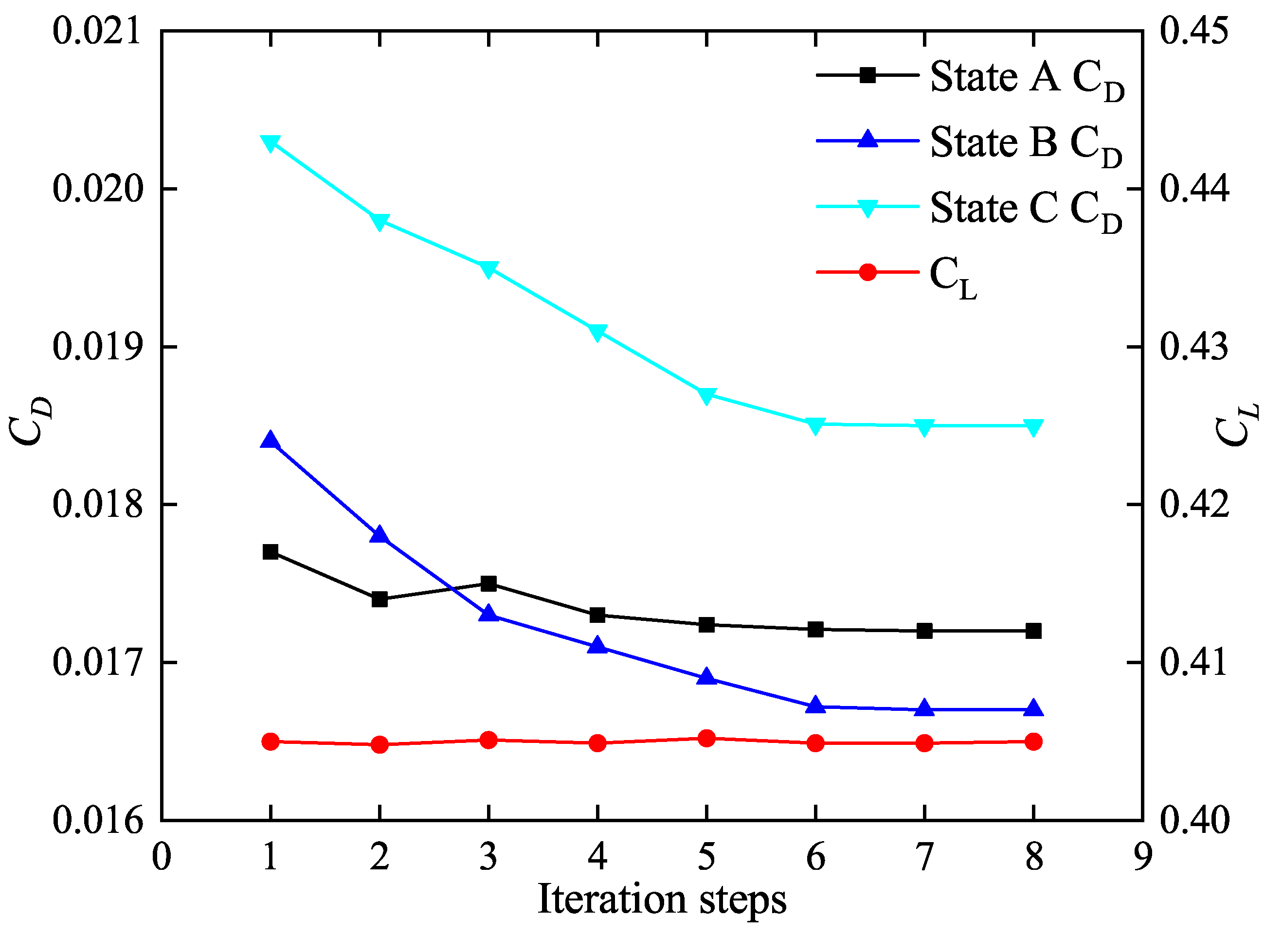
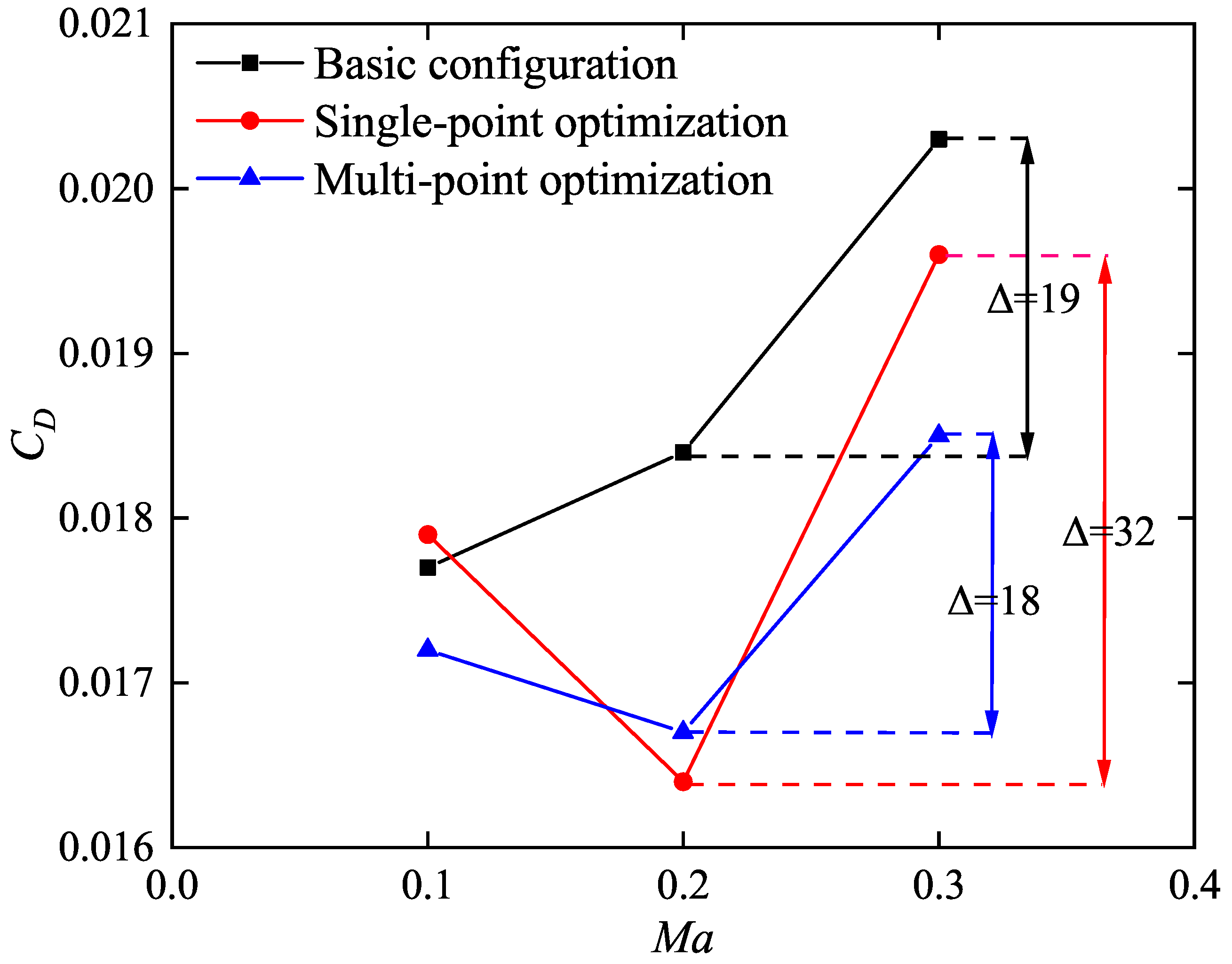
4.2. Optimal Design Problem Configuration Two

As shown in

Table 3. Design States for Optimization Configuration Two.

Design State	Ma	${\mathit{C}}_{\mathit{L}}$
A (Cruise)	0.2	0.405
B	0.4	0.432
C	0.7	0.498

, three design states are given: low speed, subsonic speed, and transonic speed.

The optimization design problem is described as follows: Objective: $minf\left(x\right)={\sum }_{i=A,B,C}{W}_i{C}_D$

Design Variables: $Z_{wing},{\alpha }_i$

Constraints: $C_L=C_{L,\mathrm{init}},\left|C_{M_y,A,B,C}\right|\le C_{M_y,A_{\mathrm{init}},B_{\mathrm{init}},C_{\mathrm{init}}},T_1\ge T_{\mathrm{init}},T_2\ge T_{\mathrm{init}},T_3\ge T_{\mathrm{init}},T_4\ge T_{\mathrm{init}}$.

The weight control parameters $W_A$, $W_B$, and $W_C$ corresponding to design states A, B, and C are each set to 0.5.

The optimization process converges by the 9th step, as shown in Figure 12. It can be observed that the lift coefficient remains nearly unchanged, while the drag coefficient decreases for all three design states.

The basic configurations of the three design states and the aerodynamic coefficients for the results of single-point and multi-point optimization are shown in

Table 4. Comparison of Aerodynamic Coefficients for Optimization Configuration Two.

Configuration	$\mathit{Ma}$	${\mathit{C}}_{\mathit{L}}$	${\mathit{C}}_{\mathit{D}}$	${\mathit{C}}_{\mathit{L}}/{\mathit{C}}_{\mathit{D}}$	$\sqrt{{\mathit{C}}_{\mathit{L}}}/{\mathit{C}}_{\mathit{D}}$	${\mathit{C}}_{\mathit{My}}$	$\mathit{\alpha }{(}^{\circ })$
Basic Configuration	0.2	0.405	0.0184	22.01	34.59	−0.00511	8.36
	0.4	0.432	0.0227	19.03	29.06	−0.00313	6.46
	0.7	0.498	0.0261	19.08	27.05	−0.00270	3.61
Single-Point Optimization	0.2	0.405	0.0164	24.70	38.82	−0.000485	10.56
	0.4	0.432	0.0164	26.34	40.23	−0.000891	8.66
	0.7	0.498	0.0244	20.41	28.93	−0.000595	5.81
Multi-Point Optimization	0.2	0.405	0.0167	24.25	38.10	0.00225	12.11
	0.4	0.432	0.0205	21.07	32.18	−0.00216	10.21
	0.7	0.498	0.0238	20.92	29.66	−0.00143	7.36

.

It can be seen that the pitching moment coefficients of each calculated state meet the constraint conditions, and the thickness of each section also satisfies the constraints. The drag coefficient for the multi-point optimization configuration decreases by 9.24% in cruise state A, 9.69% in subsonic state B, and 8.81% in transonic state C. The aerodynamic performance of each design state is improved. Since the optimization weights are set identically, the drag coefficients for each design state decrease to a similar degree. For the single-point optimization configuration, the drag coefficient decreases by 10.87% in cruise state A, 8.37% in subsonic state B, and 6.51% in transonic state C. Because optimization configuration two has a higher weight coefficient than configuration one, it compensates for non-design point issues, indicating that the optimization weight is relatively high and the optimization effect is better. Additionally, drag divergence is improved.

The comparison of the pressure contour for the transonic state of optimization configuration two is shown in Figure 13. It can be observed that the shock wave intensity in the outer wing segment decreases significantly, and the low-pressure area reduces.

5. Conclusions and Future Works

Based on the research conducted, the following conclusions can be drawn:

The drag coefficients of each design state for both configuration one and configuration two have been reduced, and the drag divergence performance has been improved. After optimization, the low-pressure region in the upper surface pressure distribution is significantly reduced, the reverse pressure gradient is alleviated, the phenomenon of flow separation is mitigated, and overall aerodynamic efficiency is enhanced.

For optimization configuration one, it was observed that although single-point optimization outperforms multi-point optimization in terms of cruise state performance, it performs poorly in reducing drag at non-design points. On the other hand, optimization configuration two demonstrates that increasing the weight coefficient helps to balance the performance issues at non-design points, leading to an improved overall optimization when the weight coefficient is high.

Multi-point optimization allows for simultaneous consideration of multiple design states, effectively improving the aerodynamic performance of both the cruise state and non-design points. This results in better comprehensive aerodynamic performance.

The discrete adjoint aerodynamic shape optimization method presented in this paper successfully addresses large-scale design variables and multi-constraint problems. It is suitable for low Mach number, subsonic, and transonic conditions, and is capable of solving practical engineering challenges. The effectiveness and robustness of this method have been demonstrated, making it widely applicable to aircraft design.

However, there are some limitations to the current approach. The method relies on RANS-based modeling, which may not fully capture unsteady effects or shock–boundary layer interactions, particularly in the transonic regime. Additionally, the structural deformation effects are not considered, limiting the scope for aero-structural optimization. The optimization process was based on only three design points, and increasing the number of design points would provide a more accurate representation of the variations across a broader operational envelope.

Future research can focus on addressing these limitations by extending the method to include aero-structural coupling using coupled adjoint methods, which would better account for the interaction between aerodynamic and structural changes. Incorporating uncertainty quantification in multi-point optimization would improve robustness and allow for better handling of variations in operational conditions. Finally, expanding the framework to cover a wider range of operating conditions, such as climb, descent, and maneuver scenarios, would allow a more comprehensive assessment of aerodynamic performance throughout the operational envelope.

References

1. Sun, Y.; Wang, Y.; Cheng, W.; Wang, M.X.; Yang, M. Analysis and Prospect of Blended-Wing-Body Configuration Technology Development of Civil Aircraft. Aeronaut. Sci. Technol. 2023, 34, 1–12. [Google Scholar] [CrossRef]
2. Wang, G.; Zhang, B.Q.; Zhang, M.H.; Sang, W.M.; Yuan, C.S. Research progress and prospect for conceptual and aerodynamic technology of blended-wing-body civil aircraft. Acta Aeronaut. Astronaut. Sin. 2019, 40, 623046. [Google Scholar]
3. Lei, G.D.; Xu, Y. Development Directions and Key Design Technologies Research of Future Large Airliners. Aeronaut. Manuf. Technol 2023, 66, 26–37. [Google Scholar] [CrossRef]
4. Jameson, A. Aerodynamic design via control theory. J. Sci. Comput. 1988, 3, 233–260. [Google Scholar] [CrossRef]
5. He, P.; Mader, C.A.; Martins, J.R.; Maki, K.J. An aerodynamic design optimization framework using a discrete adjoint approach with OpenFOAM. Comput. Fluids 2018, 168, 285–303. [Google Scholar] [CrossRef]
6. Thomas, J.P.; Dowell, E.H. Discrete adjoint approach for nonlinear unsteady aeroelastic design optimization. AIAA J. 2019, 57, 4368–4376. [Google Scholar] [CrossRef]
7. Abergo, L.; Morelli, M.; Guardone, A. Aerodynamic shape optimization based on discrete adjoint and RBF. J. Comput. Phys. 2023, 477, 111951. [Google Scholar] [CrossRef]
8. Ma, C.; Huang, J.; Li, D.; Deng, J.; Liu, G.; Zhou, L.; Chen, C. Discrete Adjoint Optimization Method for Low-Boom Aircraft Design Using Equivalent Area Distribution. Aerospace 2024, 11, 545. [Google Scholar] [CrossRef]
9. Belda, M.; Hyhlík, T. Interactive Airfoil Optimization Using Parsec Parametrization and Adjoint Method. Appl. Sci. 2024, 14, 3495. [Google Scholar] [CrossRef]
10. Liu, X.D.; Zhang, P.L.; He, G.H.; Wang, Y.E.; Yang, X.D. Multi-objective aerodynamic optimization of flying wing configuration based on adjoint method. J. Northwestern Polytech. Univ. 2021, 39, 753–760. [Google Scholar] [CrossRef]
11. Lei, R.W.; Bai, J.Q.; Xu, D.Y.; Zhang, Y.; Wang, H. Speciality assessment of sequential and concurrent aerostructural optimization based on coupled adjoint technique. J. Aerosp. Power 2019, 34, 1036–1049. [Google Scholar]
12. Zhang, W.Q.; Song, M.H.; Wang, H. Exploration on the adjoint aerodynamic optimization of a business jet considering intake and exhaust effects. Flight Dyn. 2022, 40, 8–13. [Google Scholar] [CrossRef]
13. Li, M.; Chen, J.J.; Zhou, H.; Cheng, Y.W.; Bai, J.Q. Adjoint-based aero/stealth optimization design for UAV. Acta Aeronaut. Astronaut. Sin. 2024, 45. [Google Scholar]
14. Wang, S.Y.; Yang, A. Steady/Unsteady Aerodynamic Optimization Design of Airfoil Based on Discrete Adjoint Method. J. Fudan Univ. (Nat. Sci.) 2024, 63, 209–215. [Google Scholar] [CrossRef]
15. Wong, W.S.; Moigne, A.L.; Qin, N. Parallel adjoint-based optimisation of a blended wing body aircraft with shock control bumps. Aeronaut. J. 2007, 111, 165–174. [Google Scholar] [CrossRef]
16. Abu-Zurayk, M.; Brezillon, J. Aero-Elastic Multipoint Optimization Using the Coupled Adjoint Approach. In New Results in Numerical and Experimental Fluid Mechanics IX; Springer International Publishing: Cham, Switzerland, 2014. [Google Scholar]
17. Economon, T.D.; Palacios, F.; Copeland, S.R.; Lukaczyk, T.W.; Alonso, J.J. SU2: An open-source suite for multiphysics simulation and design. AIAA J. 2016, 54, 828–846. [Google Scholar] [CrossRef]
18. Suder, K. Overview of the NASA environmentally responsible aviation project’s propulsion technology portfolio. In Proceedings of the 48th AIAA/ASME/SAE/ASEE Joint Propulsion Conference & Exhibit, Atlanta, GA, USA, 30 July–1 August 2012; p. 4038. [Google Scholar]
19. Menter, F.R. Two-equation eddy-viscosity turbulence models for engineering applications. AIAA J. 1994, 32, 1598–1605. [Google Scholar] [CrossRef]
20. Jameson, A.; Schmidt, W.; Turkel, E. Numerical solution of the Euler equations by finite volume methods using Runge Kutta time stepping schemes. In Proceedings of the 14th Fluid and Plasma Dynamics Conference, Palo Alto, CA, USA, 23 June–25 June 1981; p. 1259. [Google Scholar]
21. Sarlak, H.; Mikkelsen, R.; Sarmast, S.; Sørensen, J.N. Aerodynamic behaviour of NREL S826 airfoil at Re = 100,000. J. Phys. Conf. Ser. 2014, 524, 012027. [Google Scholar] [CrossRef]
22. Schmitt, V.; Charpin, F. Pressure distributions on the ONERA M6-wing at transonic mach numbers. In Experimental Data Base for Computer Program Assessment; Report of the Fluid Dynamics Panel Working Group 04; AGARD AR-138; NATO: Brussels, Belgium, 1979. [Google Scholar]
23. Mani, M.; Ladd, J.; Cain, A.; Bush, R.; Mani, M.; Ladd, J.; Cain, A.; Bush, R. An assessment of one-and two-equation turbulence models for internal and external flows. In Proceedings of the 28th Fluid Dynamics Conference, Snowmass Village, CO, USA, 29 June–2 July 1997; p. 2010. [Google Scholar]
24. Martineau, D.; Stokes, S.; Munday, S.; Jackson, A.; Gribben, B.; Verhoeven, N. Anisotropic hybrid mesh generation for industrial RANS applications. In Proceedings of the 44th AIAA Aerospace Sciences Meeting and Exhibit, Reno, NV, USA, 9–12 January 2006; p. 534. [Google Scholar]
25. Sederberg, T.W.; Parry, S.R. Free-form deformation of solid geometric models. In Proceedings of the 13th Annual Conference on Computer Graphics and Interactive Techniques, Dallas, TX, USA, 18–22 August 1986; pp. 151–160. [Google Scholar]
26. Anderson, W.K.; Venkatakrishnan, V. Aerodynamic design optimization on unstructured grids with a continuous adjoint formulation. Comput. Fluids 1999, 28, 443–480. [Google Scholar] [CrossRef]
27. Nadarajah, S.K.; Jameson, A. Optimum shape design for unsteady flows with time-accurate continuous and discrete adjoint method. AIAA J. 2007, 45, 1478–1491. [Google Scholar] [CrossRef]
28. Xiong, J. Aerodynamic Optimization Design Based on Response Surface Methodology; Northwestern Polytechnical University: Xi’an, China, 2006; pp. 232–236. [Google Scholar]
29. COAKLEY, T. Numerical simulation of viscous transonic airfoil flows. In Proceedings of the 25th AIAA Aerospace Sciences Meeting, Reno, NV, USA, 24–26 March 1987; p. 416. [Google Scholar]
30. Aprovitola, A.; Aurisicchio, F.; Di Nuzzo, P.E.; Pezzella, G.; Viviani, A. Low speed aerodynamic analysis of the N2A hybrid wing–body. Aerospace 2022, 9, 89. [Google Scholar] [CrossRef]
Figure 1. N2A aircraft model. (a) Realistic configuration. (b) Simulated configuration.
Aerospace 12 00404 g001
Figure 2. N2A grid. (a) Global grid. (b) Fuselage detail.
Aerospace 12 00404 g002
Figure 3. Validation results. (a) NREL S826 airfoil. (b) ONERA M6 wing.
Aerospace 12 00404 g003
Figure 4. Mesh independence analysis. (a) Lift coefficient. (b) Drag coefficient.
Aerospace 12 00404 g004
Figure 5. Validation of adjoint gradient accuracy. (a) RAE 2822 airfoil. (b) NACA 0012 airfoil.
Aerospace 12 00404 g005
Figure 6. FFD boxes.
Aerospace 12 00404 g006
Figure 7. Convergence process for Optimization Configuration One.
Aerospace 12 00404 g007
Figure 8. Drag Coefficient Divergence Curves for Each Configuration.
Aerospace 12 00404 g008
Figure 9. Wing Section Geometry and Pressure Coefficients for Optimization Configuration One. (a) Wing Section Geometry. (b) Pressure Coefficients.
Aerospace 12 00404 g009
Figure 10. Upper Wing Pressure Contour for Cruise State of Optimization Configuration One. (a) Before Optimization (b) After Optimization.
Aerospace 12 00404 g010
Figure 11. Pressure Coefficient Distribution for Each Profile in Three Design States of Optimization Configuration One. (a) Section One; (b) Section Two; (c) Section Three; (d) Section Four.
Aerospace 12 00404 g011
Figure 12. Convergence Process for Optimization Configuration Two.
Aerospace 12 00404 g012
Figure 13. Upper Wing Pressure Contour for Transonic State of Optimization Configuration Two. (a) Before Optimization (b) After Optimization.
Aerospace 12 00404 g013