End-to-End Deep-Learning-Based Surrogate Modeling for Supersonic Airfoil Shape Optimization

Abstract

Aerodynamic shape design optimization faces challenges due to the computational demands and the vast design space, limiting its practicality and scalability. While progress has been made in subsonic and transonic regimes, the real-time optimization for supersonic conditions remains unexplored. To bridge this gap, this work exploits knowledge learned from subsonic and transonic real-world data and introduces a rapid optimization framework tailored for the supersonic regime. A novel end-to-end multitask Convolutional Neural Network is proposed to predict the aerodynamic coefficients of an airfoil shape, extracting global and local features directly from the geometry. The surrogate model is thoroughly examined and validated, including an analysis of model explainability. The surrogate model achieves on par results with the state-of-the-art, with relative errors in aerodynamic coefficient predictions below 1.7%. Furthermore, a surrogate-based optimization strategy integrates the surrogate model with a Generative Adversarial Network to generate realistic airfoil shapes, thereby reducing the design space to a low-dimensional representation. This approach provides a robust solution that accelerates the optimization routine by over 3000 times when compared to simulation-based methods while achieving a deviation of less than 1.9% from their optimum performance. Overall, this work strikes a balance between efficiency and effectiveness without compromising reliability.

1. Introduction

Aerodynamic Shape Optimization (ASO) aims to enhance aerodynamic design by automating the process through integrating aerodynamic analysis and numerical optimization. However, the computational requirements for finding optimal design parameters, often using physics-based models like Computational Fluid Dynamics (CFD) simulations, can be resource-intensive and time-consuming. This challenge is amplified by the high dimensionality of the design space, making it challenging to explore and discover optimal solutions [1]. To address these limitations, Surrogate-based Optimization (SBO) has gained prominence in ASO. SBO utilizes Surrogate Models (SMs) that approximate the objective or constraint functions with improved computational efficiency compared to CFD simulations. By leveraging available aerodynamic design data, SMs enhance the efficiency of ASO [2].

In airfoil shape optimization, optimizing the airfoil surface coordinates directly is challenging due to the curse of dimensionality associated with exploring a large design space [3]. Additionally, the amount of data needed to model the high-dimensional space formed by individual points makes it intractable to train an SM capable of guiding the optimization algorithm [4]. Therefore, the SBO framework necessitates a compact parameterization for the airfoil shape. This parameterization should have the capability to represent a diverse range of shapes while avoiding the complexities of high-dimensional design spaces [5]. Moreover, training the surrogate model to predict aerodynamic coefficients for abnormal shapes would be highly inefficient. Hence, it becomes essential to establish a method that excludes abnormal shapes from consideration, enabling the cost-effective development of the SM [6,7]. Data-driven models, such as modal parameterization and design space filtering, have emerged as innovative techniques that leverage data from traditional designs to represent a wide variety of airfoils. Modal parameterization offers simultaneous control over the entire geometry of the airfoil by leveraging the representative modes derived from an airfoil shape database. Compared to conventional methods, this approach demonstrates higher accuracy in reconstructing airfoil geometries [8]. Modal parameterization methods have been developed to capture the dominant modes in airfoil shapes. Linear modes are captured using Principal Component Analysis (PCA) [9,10,11,12,13], while Variational Autoencoders (VAEs) [14,15] and Generative Adversarial Networks (GANs) [3,6,7,16] can capture both linear and nonlinear modes. In addition, design space filtering techniques have been proposed to mitigate geometric abnormalities within the design space. These techniques employ constraint functions to evaluate the abnormality of samples and subsequently restrict the design space accordingly [11,12,16,17,18,19,20].

In the field of ASO, SMs can be trained using datasets from simulations or experiments to predict aerodynamic coefficients. Traditional SMs, such as Kriging [21] and its variants [22,23,24], faced limitations in handling large training datasets [22]. However, recent advancements in Deep Learning (DL) models have addressed this issue [3,7,12,25,26,27]. Once the initial training database adequately represents the design space, the SM is expected to guide the entire optimization process after a single training step. Real-world airfoils, such as those from the University of Illinois Urbana-Champaign (UIUC) Aerofoil Coordinates Database [28], can serve as valuable resources for training accurate SMs in airfoil shape design [7,11,12,24,26,29]. These advancements in surrogate modeling have led to increasingly effective and efficient models, empowering engineers to engage in interactive ASO with near real-time optimization routines. Different techniques have been proposed, including the mixture of experts with gradient-enhanced Kriging [11], gradient-enhanced Multilayer Perceptron (MLP) [7,12,25,30], Long Short-Term Memory (LSTM) [7], and Convolutional Neural Network (CNN) [3,26,27,29].

This study aims to fill the existing research gaps in the field of ASO by focusing on the supersonic regime. While notable advancements have been made in subsonic and transonic conditions, there remains a lack of studies addressing interactive ASO in supersonic conditions. This scarcity of research may be due to limited data availability and increased complexities in modeling nonlinearities within the supersonic regime. Consequently, the objective of this work is to develop a modeling approach for supersonic airfoil data, enabling the implementation of a real-time ASO routine tailored to two-dimensional airfoils. To accomplish this goal, the following proposals are put forth in this work:

• a novel, end-to-end DL-based SM trained on openly accessible subsonic and transonic airfoil geometric data to predict aerodynamic coefficients from airfoil coordinates, for guiding the optimization routine in supersonic conditions;
• an InfoGAN trained to represent an aerodynamically valid design space that includes shapes suited for subsonic, transonic and supersonic conditions;
• a modular, real-time-capable optimization framework that integrates the SM with the generative design space representation, enabling rapid ASO for supersonic conditions.

The remainder of this document is organized as follows. Section 2 offers a description of the methodology employed, while Section 3 presents and analyses the results obtained through the implementation of the proposed framework, along with a benchmark against state-of-the-art techniques. Lastly, Section 4 provides an overview of the achievements of this work.

2. Methodology

This section provides an overview of the proposed SBO framework for supersonic airfoil shapes, followed by a detailed discussion of its three core modules. Firstly, it discusses the selection of a suitable geometry parameterization. Next, it delves into the novel SM architecture that is proposed. Lastly, it covers the optimization algorithm that has been chosen for the framework.

2.1. Overview

The proposed framework for real-time airfoil shape optimization is comprised of three primary modules. The first module employs an Information Maximizing Generative Adversarial Network (InfoGAN) to parameterize the airfoil geometry in a latent space consisting of incompressible noise, $\mathit{z}$, and latent codes, $\mathit{c}$ [31]. This parameterization enables the representation of the airfoil geometry in a low-dimensional space, facilitating the efficient generation of airfoils using the generator network. The second module is a CNN, which maps the geometry of an airfoil, $\mathit{Y}$, and its Angle of Attack (AoA), $\alpha$, to its corresponding aerodynamic coefficients, $C_d$ and $C_l$, in supersonic conditions, without the need for costly physics-based simulations. These first two modules work sequentially to complete the mapping between the parameter space and the corresponding aerodynamic coefficients. The third module is the optimization solver, which takes advantage of this end-to-end mapping to optimize a given objective function, subject to aerodynamic and geometric constraints, by exploring the parameter space with a Genetic Algorithm (GA). Figure 1 provides a visual representation of the workflow of the proposed framework.

2.2. Airfoil Geometry Parameterization

A nonlinear modal parameterization is employed to model the data-generating distribution of real-world airfoil shapes from UIUC, ensuring both shape diversity and validity. Nonlinear modal parameterizations are particularly advantageous as they retain nonlinear information from the data and facilitate defining boundaries for the design variables [6,7]. The InfoGAN is utilized for this purpose, where the generator is trained to generate disentangled shape modes by assigning meaning to its latent codes, $\mathit{c}$ [31]. By employing the InfoGAN, this framework addresses the high-dimensional nature of ASO problems while ensuring the variety of the generated shapes. The InfoGAN architecture used in this work is similar to the one proposed by Chen et al. [6].

2.3. Aerodynamic Coefficients Surrogate Modeling

Surrogate modeling often involves constructing a model that maps the parameter space to the aerodynamic coefficients of an airfoil [7,11,12,18,24]. However, this approach may lack robustness in the absence of prior knowledge about optimal shapes in supersonic conditions. To address this limitation, a novel end-to-end approach is proposed. Instead of relying on features derived from shape parameterization, the proposed approach delegates feature extraction to the model responsible for predicting aerodynamic coefficients, enabling it to autonomously learn the most relevant features for the task it is trained to perform [33]. With each model trained on distinct objectives, one focused on design space representation and the other on coefficient regression, this setup promotes robust feature learning directly from raw airfoil geometry data to predict aerodynamic coefficients, $C_d$ and $C_l$. This strategy resembles a CFD-based framework, wherein the geometry parameterization reconstructs the airfoil geometry based on the design variables, allowing it to be simulated by CFD methods [34]. Figure 2 illustrates a comparison between the state-of-the-art and the proposed strategies.

In this study, a CNN is implemented based on the assumption that spatial and locality information play a crucial role in feature extraction. The input to the model consists of the vertical coordinates of the airfoil surfaces organized in a matrix format $\mathit{Y}$. This approach offers advantages in terms of incorporating thickness and curvature information and being independent of the parameterization. To further improve the internal representations of the airfoil geometry, a multitask network is utilized, enabling the model to complement the learned features for both $C_d$ and $C_l$. The flow conditions are considered through a late fusion approach, with only the AoA taken into account in this work. As outlined in Section 2.4, the optimization is conducted with constant Mach and Reynolds numbers ($M=2$ and $Re=3.7\times {10}^6$), eliminating the need for these as explicit inputs.

Hence, the proposed CNN architecture comprises a multi-branch backbone with multiple convolutional blocks running in parallel with fully connected layers, which are combined with a residual connection. The AoA is also concatenated at this stage. Finally, the architecture includes a decoder. The overall design is illustrated in Figure 3.

The convolutional blocks consist of convolutional layers, followed by batch normalization [35], Leaky ReLU (Rectified Linear Unit) activation functions [36], and dropout [37]. The use of convolutional layers is preferred as they efficiently learn local features [33], such as thickness and curvature, across the airfoil geometry. Strided convolutions are selected over deterministic spatial pooling functions for reducing feature maps, as they preserve precise spatial information by maintaining translation equivariance [33]. The residual connection with the input transformation by a fully connected layer serves two purposes. First, to use the fully connected layer to model information from distant locations, enabling the extraction of global features from the shape that cannot be learned with a convolutional layer, and second, to improve the network learning capabilities by refining the internal representations of the input [38]. The decoder processes two signals: the residually connected local and global features extracted from the airfoil geometry, and the flow conditions with the AoA. By combining these features through fully connected layers, it can map them into the two aerodynamic coefficients $C_d$ and $C_l$, allowing for a multitask architecture.

2.4. Optimization Algorithm

In order to complete the optimization framework for the supersonic ASO, a gradient-free optimization scheme is employed. This choice is motivated by the presence of shock wave-induced gradient discontinuities that can compromise the accuracy of aerodynamic coefficient gradient predictions by the SM [12]. Despite potential challenges such as longer convergence times and scalability issues, the low dimensionality of the design space and the efficiency of the SM make the GA well-suited for this problem, as they prioritize exploration for global search, increasing the likelihood of obtaining optimal solutions [4]. GAs are most directly suited to unconstrained optimization problems. However, by using penalty functions [39], GAs can be extended to handle constrained optimization problems.

3. Numerical Results and Discussion

This section begins by providing a definition of the case study, which involves the minimization of a lifting surface. It then proceeds to outline the development process for the DL models utilized within the optimization framework. The process encompasses several steps, such as database creation, training, and validation procedures. Lastly, the effectiveness of the proposed methodology is evaluated by applying it to the case study.

3.1. Problem Formulation

In order to demonstrate the capabilities of the proposed framework in supersonic ASO, a specific case study is conducted, without loss of generality. The chosen optimization problem focuses on minimizing drag for an airfoil shape at a freestream Mach number, M, of 2.0, Reynolds number, $Re$, of 3.7 × 10⁶, subject to a minimum area of $A^{\ast }$ and a lift coefficient of $C_l^{\ast }$, with respect to the airfoil shape, $\mathit{Y}$, and AoA, $\alpha$. In summary, the optimization problem can be expressed as

$$\begin{array}{ccc}\hfill \underset{\mathit{Y},\alpha }{min}& \hfill & C_d(\mathit{Y},\alpha ),\hfill \\ \hfill subject\; to:& \hfill & A\left(\mathit{Y}\right)\ge A^{\ast }\left(\mathit{Y}\right),\hfill \\ \hfill & \hfill & C_l(\mathit{Y},\alpha )=C_l^{\ast }(\mathit{Y},\alpha ),\hfill \\ \hfill & \hfill & M=2.0,\hfill \\ \hfill & \hfill & Re=3.7\times {10}^6.\hfill \end{array}$$

(1)

This problem is inspired by the drag minimization of the RAE 2822 in transonic viscous flow, as defined by the Aerodynamic Design Optimization Discussion Group (ADODG) [5,34].

3.2. DL Models Development

3.2.1. Data Collection

To develop the SM, it is necessary to have a database comprising pairs of geometry and aerodynamic coefficients. However, since there is a lack of real-world geometric data suitable for supersonic conditions, an extensive database from the UIUC library, which primarily consists of real airfoils for subsonic and transonic applications, is utilized to establish a framework for generating optimal supersonic airfoils. The aerodynamic coefficients of these airfoil shapes are obtained through CFD simulations at multiple AoAs, thereby completing the SM database. Despite the potential for generating a more extensive database, a computational budget has been established to confine the simulated geometries to those present in the UIUC database.

Before simulating the airfoil geometries, a preprocessing step is executed to standardize the distribution of their coordinates. This step follows a similar approach proposed by Li et al. [11] and involves employing a cosine spacing distribution with 128 points on each surface. The simulations are carried out using pyHyp version v2.6.1 [40] for hyperbolic mesh generation and the approximate Newton–Krylov (ANK) solver [41] integrated within ADflow v2.12.1 [42] for CFD simulations. An $L^2$ convergence criterion of 10⁻⁸ is employed. The steady RANS equations, along with the Spalart–Allmaras turbulence model [43], are used for solving the simulations.

In order to ensure consistent accuracy in simulations throughout the entire database, a mesh convergence study is carried out to determine the most suited mesh resolution for all airfoils. This study assesses the discretization error in the aerodynamic coefficients of the NACA 0012 airfoil at an AoA of 1.5° through iterative mesh coarsening in streamline and off-wall directions [44]. Although it is not ideal to use the same mesh configuration for such a vast number of airfoils and different AoAs, defining the best grid for each airfoil and AoA individually would be intractable. Therefore, the mesh determined by the mesh convergence study with NACA 0012, represented in Figure 4, serves as the standard mesh for simulating every airfoil in the database.

The results presented in

Table 1. Mesh convergence study performed with NACA 0012 at an AoA of 1.5°, M of 2 and $Re$ of 3.7 × ${10}^6$. The drag coefficient $C_d$ of the multiple mesh configurations is compared with the Richardson extrapolation. One $C_d$ count corresponds to ${10}^{-4}$ and one $C_l$ count to ${10}^{-3}$. The CPU time taken to generate the mesh and to perform the CFD simulation is measured from a workstation provided with an Intel Core i9-11900 processor.

Nodes in Off-Wall Direction	Number of Cells	${\mathit{C}}_{\mathit{l}}$ Counts	${\mathit{C}}_{\mathit{d}}$ Counts	Extrapolated Relative ${\mathit{C}}_{\mathit{d}}$ Error	CPU Time [s]
2048	499,468	55.07	973.7	0.01%	2.4 × ${10}^4$
512	124,684	55.09	974.0	0.04%	2.3 × ${10}^3$
128	30,988	55.14	975.9	0.23%	8.7 × ${10}^1$
Richardson extrapolation		-	973.2	-	-

demonstrate that increasing the number of cells leads to a higher CPU time while maintaining high accuracy across all mesh configurations. Based on the scalability of computational cost and accuracy achieved, an O-mesh with 128 nodes in the off-wall direction is selected for simulating the complete airfoil dataset. This decision takes into account the requirement for conducting a large number of simulations. To capture the viscous effects and dissipate the energy generated near the airfoil before it reaches the far field, a thickness of the first layer of $6.5\times {10}^{-6}$ m and a distance of 500 airfoil chords between the first and last layers are utilized, respectively.

3.2.2. Dataset Splitting

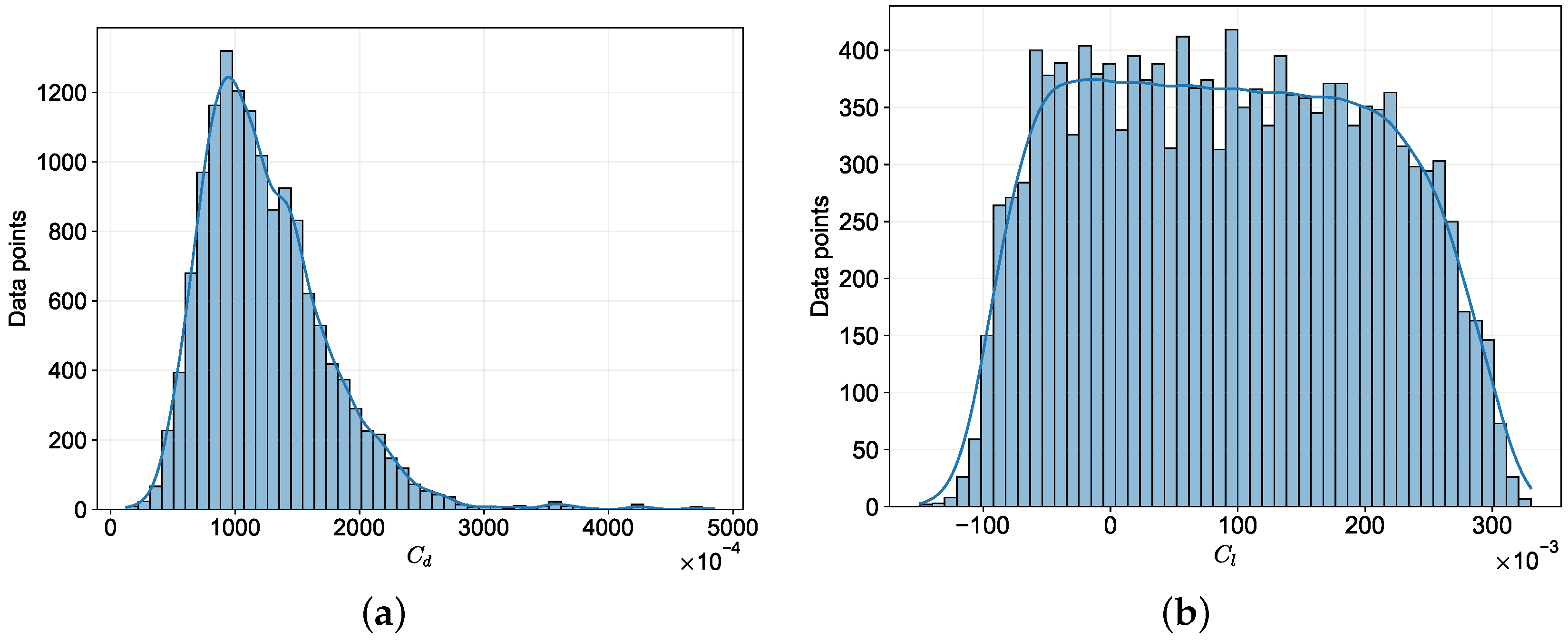
After preprocessing 1600 airfoils from the UIUC library, 1411 geometries are deemed suitable for use in the DL models. The remaining geometries are excluded due to missing data or because the CFD simulations failed to converge, indicating they may not be appropriate for the specified M and AoA. Figure 5 depicts the distributions of aerodynamic coefficients obtained, showing a concentration of data points near 1000 $C_d$ counts, resembling a Gaussian distribution, while the $C_l$ has a more even distribution due to its linearity with the AoA.

To ensure that the SM is not overfitting the training data and to evaluate its performance and generalization capabilities, the 1411 airfoils are randomly divided into training (80%), validation (10%), and test (10%) sets, containing 1129, 141 and 141 airfoils, respectively. Furthermore, it is important to note that each data point representing an airfoil geometry at different AoAs is exclusive to one dataset. This process is designed to prevent the SM from memorizing the performance of a geometry at certain AoAs and simply use that information to interpolate the results for other AoAs, compromising the performance analysis of the SM. The data comprise 10 different AoAs, ranging from −1° to 8°, as it was assumed that in this range the lift curve could be assumed in the linear region. As a result, the training, validation, and test sets are comprised of a total of 11,290, 1410 and 1410 samples, respectively.

Regarding the InfoGAN, all geometries are used for training. Additionally, to enhance the representation capabilities of the InfoGAN, its training set is extended with additional shapes suitable for supersonic conditions, following the approach employed by Li et al. [11] for transonic conditions. Specifically, 10 geometries from each of the biconvex [45] and B-spline [46] airfoil parameterizations are included. The biconvex airfoils are parameterized based on their area. The B-spline airfoils are generated using control points located at 10%, 50%, and 90% of the airfoil chord on each surface, as suggested by Siegler et al. [46].

3.2.3. InfoGAN Training

To ensure consistency with Chen et al. [6], the InfoGAN model is trained using the same hyperparameters and optimization algorithms. The generator network produces a 31-dimensional Bézier curve representing the airfoil. Both the discriminator and generator networks were trained using the Adam optimization algorithm [47], with a learning rate of 1 × 10⁻⁴ for 10,000 epochs and a batch size of 32. The network architectures are similar to a Deep Convolutional Generative Adversarial Network (DCGAN) [48], employing ReLU activation functions [49] and a 40% dropout probability [37]. For further details, refer to Chen et al.’s work [6].

A grid search test explored the different dimensionalities of latent codes and noise vectors, considering values of 4, 8, and 16 for each variable. The InfoGAN generator designs are evaluated using the Maximum Mean Discrepancy (MMD) metric [50]. The MMD measures how closely the generator, $p_G$, approximates the data-generating distribution, $p_{\mathrm{data}}$, with lower values indicating that the generator is better at producing realistic designs.

$${\mathrm{MMD}}^2(p_{\mathrm{data}},p_G)={\mathbb{E}}_{{\mathbf{x}}_{\mathrm{data}},{\mathbf{x}}_{\mathrm{data}}^{\prime }\sim p_{\mathrm{data}};{\mathbf{x}}_G,{\mathbf{x}}_G^{\prime }\sim p_G}\left[\kappa ({\mathbf{x}}_{\mathrm{data}},{\mathbf{x}}_{\mathrm{data}}^{\prime })-2\kappa ({\mathbf{x}}_{\mathrm{data}},{\mathbf{x}}_G)+\kappa ({\mathbf{x}}_G,{\mathbf{x}}_G^{\prime })\right],$$

(2)

where $\kappa (\mathbf{x},{\mathbf{x}}^{\prime })=e^{-\left|\right|\mathbf{x}-{\mathbf{x}}^{\prime }{\left|\right|}^2/\left(2{\sigma }^2\right)}$ is a Gaussian kernel and $\sigma$ is the kernel length scale, set to 1. The results indicated that the optimal number of latent variables for shape optimization is 8, while noise variables do not contribute significantly. This aligns with Chen et al.’s findings, where increasing latent variables take priority in capturing shape variation.

After training, the discriminator becomes obsolete since it can no longer distinguish between real and synthetic data. The generator is retained for shape generation. The training is conducted using the PyTorch 2.5.0 framework [51], resulting in an MMD value of 0.23. This represents an improvement of approximately 40% compared to the results obtained by Chen et al. [6]. The difference in performance is attributed to the training set, as the same architecture and hyperparameters are used. The main distinction between the two approaches lies in the representation of airfoils. In this work, airfoils are represented using a cosine distribution, whereas the authors used a distribution based on the curvature of the airfoil surfaces [52]. This finding suggests that the cosine distribution offers more relevant features for the network to learn from. Specifically, it provides greater discretization near the airfoil edges, which may be key regions for extracting features to represent a wide variety of airfoil shapes. Moreover, the consistent spacing of the cosine distribution can enhance the training convergence by providing uniform inputs, thereby promoting stability and consistency throughout the training process.

Furthermore, Figure 6 illustrates the primary nonlinear modes obtained from the latent codes after training the InfoGAN. These modes are responsible for the most significant changes in the airfoil shape, while the remaining latent codes produce less effective changes. For instance, the first latent code, $c_1$, primarily governs the thickness of the airfoil, while the second, $c_2$, is mostly responsible for altering the airfoil curvature. In contrast, changes to the trailing edge shape are dominated by the fourth, $c_4$, and sixth, $c_6$, latent codes. Specifically, $c_4$ controls the curvature of the lower surface near the trailing edge, while $c_6$ influences the angle of the upper surface at the trailing edge.

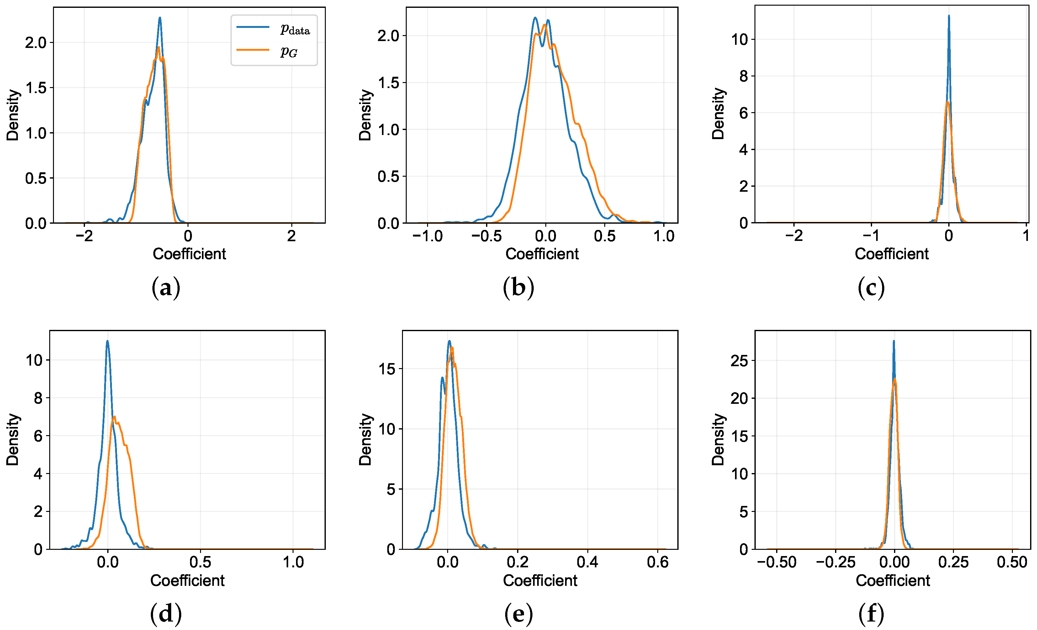
Figure 7 demonstrates that InfoGAN successfully replicates the data-generating distribution without any mode collapse issues reported in previous GAN models [18,19]. This outcome can be attributed to the simplification of the generative model task facilitated by the Bézier layer, as highlighted by Chen et al. [6]. Specifically, the generator is only required to generate the curve control points, weights, and parameter variables, as opposed to the complete airfoil surfaces. Nevertheless, there is a slight discrepancy observed in the density curve of the fourth mode between the generator, $p_G$, and the data-generating $p_{\mathrm{data}}$ distributions.

The density curve of the fourth mode shows a slight deviation between the generator and data-generation distributions. To better understand the impact of this divergence on airfoil shapes, Figure 8 illustrates the behavior of the fourth mode on an example airfoil. While it may be difficult to interpret the mode shape directly, Figure 8a,b provides a clearer understanding. By increasing the contribution from the fourth singular vector, the maximum thickness location of the airfoil is shifted towards the trailing edge. This occurs because the mode reduces the thickness of the airfoil up to 38% of the chord and then increases it downstream. Additionally, the mode induces a slight increase in the camber on account of its center line being mostly above zero. As a result, the generator synthesizes more airfoils with a rearward shift of the maximum thickness location and increased camber.

3.2.4. SM Training

The development of the aerodynamic coefficients SM involves constructing a comprehensive architecture specifically designed for this purpose. The entire process encompasses various aspects, such as data handling, training procedures, and hyperparameter choices, which are implemented using PyTorch. First, to ensure consistent gradients, the input and output data are normalized using the z-score method [35]. The Mean Squared Error (MSE) is preferred as the loss function because it penalizes higher errors, thereby facilitating the learning of aerodynamic coefficients for the best-performing shapes characterized by the highest absolute values after normalization [53]. Then, to prevent overfitting and improve model generalization, regularization techniques such as early stopping [33], batch normalization, dropout, and weight decay [33] are applied.

Furthermore, an empirical hyperparameter tuning process is employed to enhance the DL model architecture and training procedure. The hyperparameters that are tuned include the number of layers, the number of output channels of each convolution, the size of the convolutional kernel, the convolutional padding, the activation functions, the dropout percentage, the learning rate, its scheduler, the batch size, and the optimizer. The different models are trained using the training and validation datasets, and their performance is evaluated using the test dataset. The best-performing model is selected based on evaluation metrics such as the loss function and computational efficiency.

After thorough experimentation, the final architecture of the proposed DL-based SM is depicted in Figure 3. The training procedure involves utilizing the Adam optimization algorithm, renowned for its adaptive learning rate and robustness in hyperparameter tuning. A batch size of 16 is utilized, along with a learning rate of 1 × 10⁻⁴, which is adjusted using a cosine annealing with warm restarts schedule [54]. A dropout rate of 20% is applied, and decoupled weight decay [55] with a factor of 1 × 10⁻⁴ is incorporated.

The accuracy of the model on the test set is evaluated and benchmarked against the state-of-the-art in subsonic and transonic aerodynamic coefficient modeling, as shown in

Table 2. Aerodynamic coefficient modeling results for the test dataset benchmarked against state-of-the-art findings in interactive airfoil shape optimization. The presented results are provided by the respective authors.

Study	Model	Flight Condition	Training Samples	Modeling Variables	Application	${\mathsf{ϵ}}_{{\mathit{L}}^{\mathbf{2}}}$	Results RMSE (Counts)	NRMSE
Nagawkar et al. [24]	PC-Cokriging	Transonic	1074	8	$C_d$	-	6.00	2.5%
		Subsonic	81,000	16		0.26 %, 0.15%	-	-
Li et al. [11]	GE-KPLS	Transonic	32,400	10	$C_d$, $C_l$	0.83%, 0.40%	-	-
		Subsonic	42,039	16		0.32%, 0.19%	-	-
Bouhlel et al. [12]	MLP	Transonic	4120	10	$C_d$, $C_l$	0.48%, 0.28%	-	-
		Subsonic	45,696	29		2.26%, 2.34%	2.77, 12.90	0.9%, 0.9%
Du et al. [7]	MLP	Transonic	39,505	29	$C_d$, $C_l$	4.65%, 2.87%	8.76, 16.13	1.5%, 1.5%
Zhang et al. [26]	CNN	Transonic	1600	2403	$C_l$	-	70.71	-
Proposed	CNN	Supersonic	11,290	257	$C_d$, $C_l$	1.11%, 1.69%	15.50, 2.42	0.4%, 0.5%

. However, it should be noted that a direct comparison of model accuracy cannot be made, as the regimes where the aerodynamic coefficients were computed are different, resulting in different functions being emulated. Nevertheless, since the state-of-the-art has yet to attempt the solution of supersonic ASO with a real-time framework, this work compares its results with available results in subsonic and transonic aerodynamic coefficient modeling. The metrics assessed include the relative $L^2$ error,

$${ϵ}_{L^2}={\displaystyle \frac{\left|\right|\widehat{\mathbf{y}}-\mathbf{y}{\left|\right|}_2}{{\left|\right|\mathbf{y}\left|\right|}_2}},$$

(3)

where the vector $\mathbf{y}$ contains the real values, while the vector $\widehat{\mathbf{y}}$ contains the corresponding predictions, the Root Mean Squared Error (RMSE) expressed in counts,

$$\mathrm{RMSE}=\sqrt{{\displaystyle \frac{1}{N}}\sum _{i=1}^N{\left({\widehat{\mathbf{y}}}_i-{\mathbf{y}}_i\right)}^2},$$

(4)

where N is the number of examples used for computing the error, and the Normalized Root Mean Squared Error (NRMSE),

$$\mathrm{NRMSE}={\displaystyle \frac{\mathrm{RMSE}}{max\left(\mathbf{y}\right)-min\left(\mathbf{y}\right)}}.$$

(5)

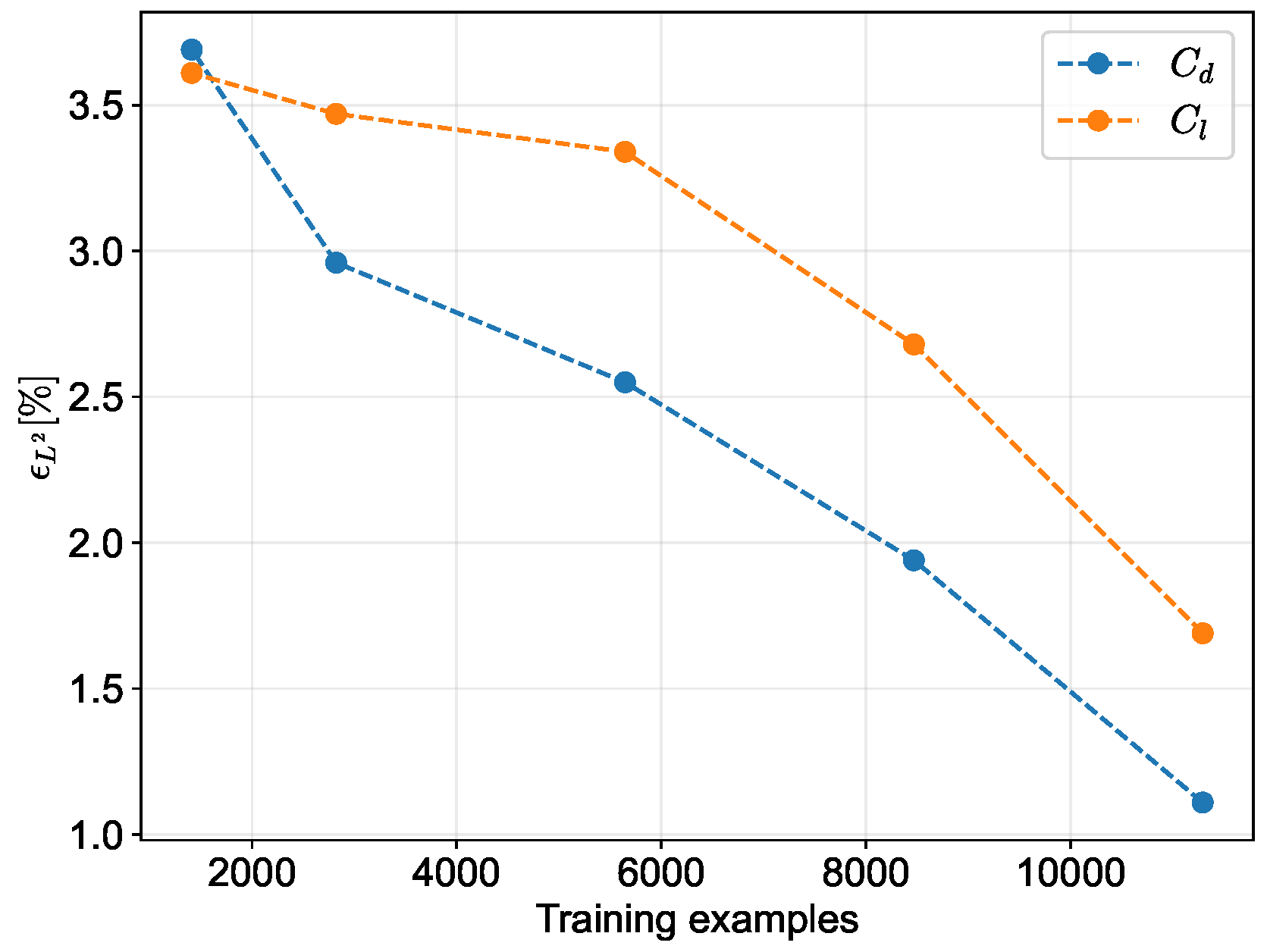
The proposed methodology attains an accuracy comparable to the state-of-the-art, achieving relative $L^2$ errors below 1.7%. Regarding the RMSEs, the proposed model exhibits a lower error in $C_l$ and a higher error in $C_d$ when compared to state-of-the-art models. However, it is important to note that in supersonic conditions, the values of $C_d$ are naturally higher due to the inclusion of wave drag [56]. When the results are normalized with the range of values found in the test dataset, the proposed model achieves NRMSEs lower than 0.5%, implying that the increased RMSE in $C_d$ relative to state-of-the-art models falls within the same spectrum. This achievement is particularly noteworthy considering the model development within a defined computational budget. Nonetheless, there is an acknowledgment of the potential for further improvements by increasing the amount of training data, as showcased by the trends depicted in Figure 9.

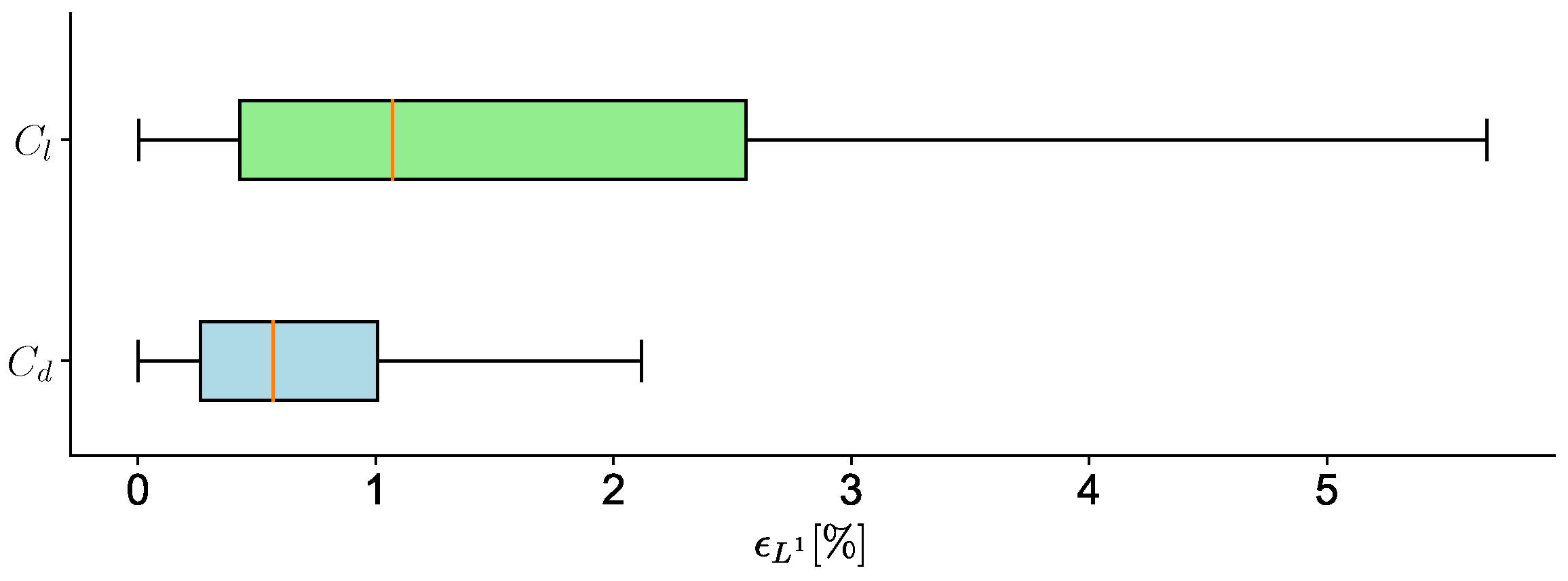
Figure 10 compares the dispersion of the relative $L^1$ error

$${ϵ}_{L^1}^{\left(i\right)}=\left|{\displaystyle \frac{{\widehat{\mathrm{y}}}_i-{\mathrm{y}}_i}{{\mathrm{y}}_i}}\right|,$$

(6)

that measures the absolute difference between the predicted value ${\widehat{\mathrm{y}}}_i$ and the actual value ${\mathrm{y}}_i$, normalized by ${\mathrm{y}}_i$. The results indicate that the error containment for $C_d$ is higher than that for $C_l$. This difference can be attributed to the fact that the distribution of $C_l$ is similar to a uniform distribution, while that of $C_d$ is closer to a Gaussian distribution, as evident from Figure 5. A uniform distribution has a flat probability density function, which can make it more challenging to be learned by the SM, as all values are equally likely.

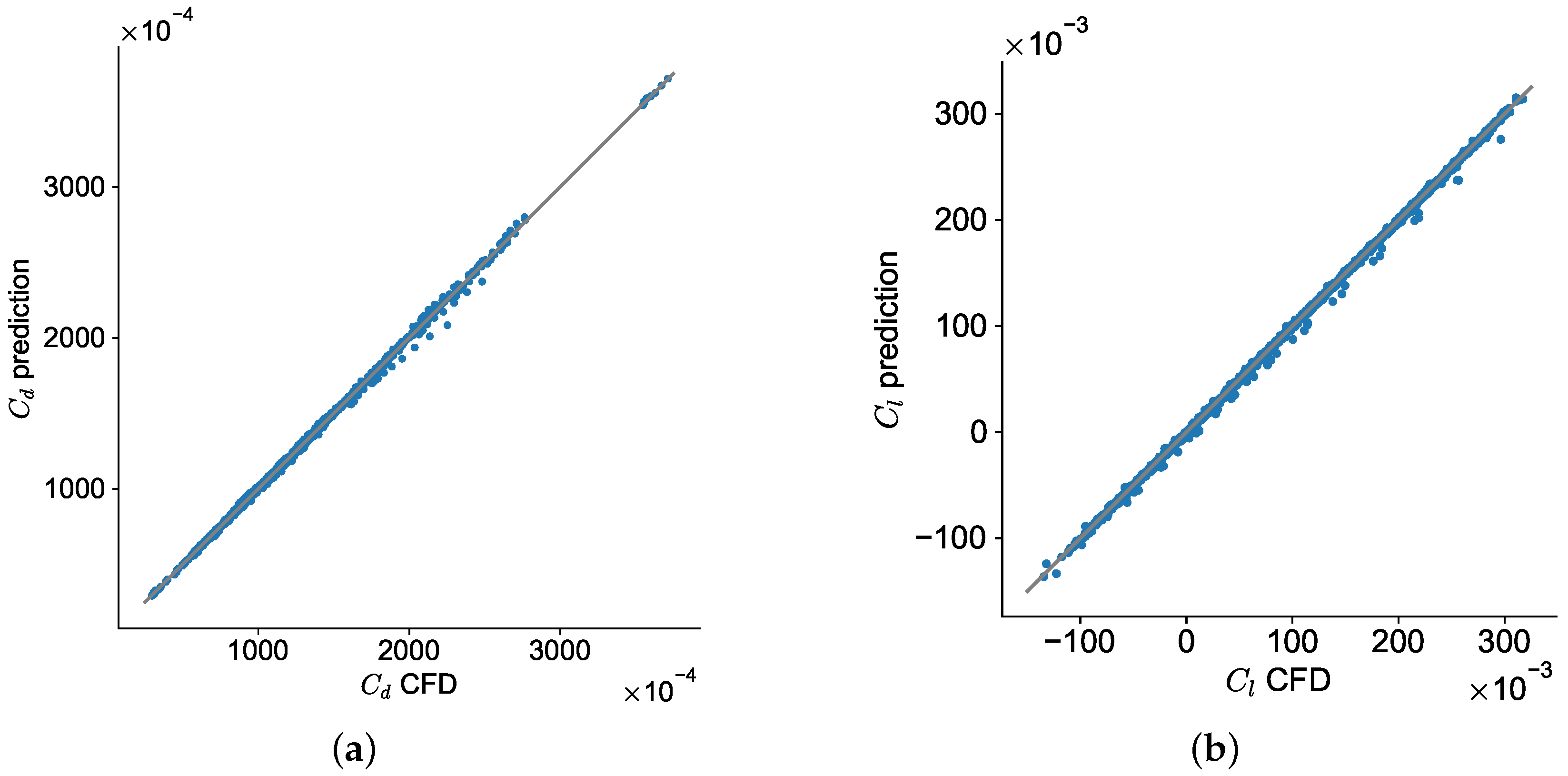
The performance of the regression model on previously unseen data is evaluated by visually comparing its predictions with the test data in Figure 11. The accuracy of the regression is indicated by the proximity of the predicted values to the actual data points, as well as by high values of the coefficient of determination $R^2$. This metric measures the proportion of the variance in the dependent variable that can be explained by the independent variables.

$$R^2=1-{\displaystyle \frac{{\sum }_{i=1}^N{\left({\widehat{\mathrm{y}}}_i-{\mathrm{y}}_i\right)}^2}{{\sum }_{i=1}^N\left({\widehat{\mathrm{y}}}_i-\overline{\mathrm{y}}\right)}}.$$

(7)

A high value of $R^2$ indicates a good fit between the model and the data, with values close to 1 indicating a strong relationship between the variables.

When developing an SM, accurately modeling high-performing airfoils and understanding underperforming shapes are crucial. This helps to avoid poor-performing regions in the design space and to guide the optimization process towards well-performing areas. In Figure 12, an analysis of the SM prediction of drag polars for airfoils with different performance levels belonging to the test set is presented. The results demonstrate that the SM performs well in predicting the first two performance levels, exhibiting higher accuracy at higher AoAs, possibly due to the linearity of the drag polar in these airfoils in this region. In contrast, the worst-performing airfoil has out-of-distribution $C_d$ values, making it challenging for the SM to generalize. Nevertheless, the prediction accuracy is sufficient to reject this airfoil for optimal design purposes. Additionally, the failure of the SM to predict the smoothness of the drag polars could be attributed to the limited granularity of AoA in the training samples, which are spaced by 1°. To enhance accuracy, particularly in low-drag and low-AoA regions where nonlinearity is more prominent, an increase in the granularity of training samples in these areas is recommended, with additional sampling at smaller AoA increments.

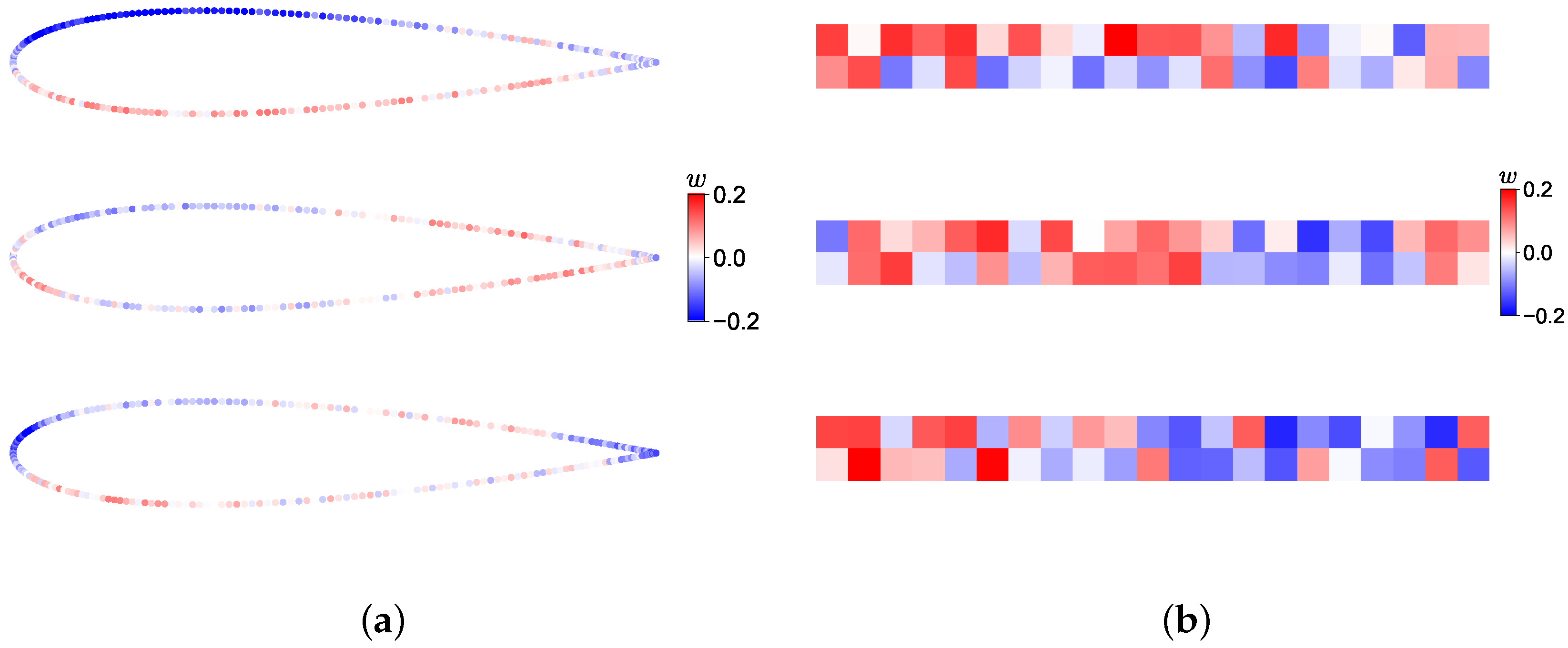
To validate the hypothesis concerning the analysis of airfoil geometry by the SM, the weights of the initial layers are examined, as illustrated in Figure 13. Although DL models are often regarded as black-box models, the aim of this work is to enhance the model’s explainability by visualizing the learned weights. This approach aids in understanding the most significant features that influence the SM predictions and their correlation with the physical characteristics of the airfoil. As expected, the fully connected layer has acquired the ability to extract global features, as shown in Figure 13a, to complement the local features derived from the convolutional layers. The first set of weights indicates that the SM has learned to assess the area of the airfoil by considering its thickness at multiple points along its geometry. The second set of weights suggests that the SM has learned a measure of the average points along the airfoil surfaces, possibly related to the camber or camber line. Lastly, the weights in the last set represent a neuron extracting combined features from the shapes of the airfoil edges. These features are only possible to extract due to the application of the fully connected layer, as the kernels of the convolutional layers do not extend to the complete shape of the airfoil. In contrast, Figure 13b provides examples of kernels from the first convolutional layer of the SM. The kernels used in the first layer have two rows to allow them to capture information from each surface individually, as well as their correlation. The learned features are more intricate and complex, without a clear pattern in the signs of their weights. Nevertheless, the kernels generally present higher values on the left side, indicating the computation of the airfoil local curvature. Some kernels exhibit positive weights on the top row and negative weights on the bottom row on the left, suggesting the extraction of the local thickness of the airfoil as the kernel passes through it. At certain locations, such as the right end of the last convolutional kernel, square patterns of positive and negative weights at the diagonals suggest the extraction of a feature related to the gradient of the airfoil thickness.

To further examine the proposed model, ablation studies were conducted on its most relevant components to decipher its most impactful attributes.

Table 3. Ablation study results for the proposed network configuration. The MLP consists of 6 fully connected layers. The second configuration consists of convolutions replacing the stride with max pooling. The third fuses the flow information to the airfoil geometry as an extra convolutional channel. The last configuration features the removal of the residual connection.

Configuration	Test MSE	Number of Parameters
MLP	1.20 × ${10}^{-3}$	0.077 M
CNN + Pooling	6.70 × ${10}^{-4}$	0.630 M
Early fusion	5.54 × ${10}^{-4}$	1.450 M
Without residual	1.41 × ${10}^{-2}$	0.474 M
Proposed	4.73 × ${10}^{-4}$	0.507 M

displays the resulting MSE values obtained from testing different configurations of the SM, where individual components were altered. The hypothesis of using strided convolutions instead of pooling to enable the network to learn its own spatial downsampling [48], and the late fusion of the flow properties produced favorable results, resulting in an increase in the SM accuracy. Notably, the convolutional blocks, which extract local features from geometry, as previously analyzed in Figure 13a, and the fully connected layer in the residual connection, which extracts global features seen in Figure 13b, play crucial roles in increasing the network’s generalization capabilities. Comparing the proposed architecture with a pure MLP with a similar architecture as that proposed by Bouhlel et al. [12] and a pure CNN without residual connection, leads to the conclusion that fusing local and global features is an effective approach for learning relevant representations of airfoil shapes for aerodynamic coefficient modeling.

Lastly, in order to ensure that the proposed method is not only capable of accurately predicting the aerodynamic coefficients of an airfoil shape but also capable of guiding the optimizer to the most suitable shapes for supersonic conditions, its performance is evaluated. Figure 14 illustrates that the proposed SM predicts the top 15 best-performing airfoil shapes from the test dataset in supersonic conditions and ranks the best 11 airfoils correctly. Although there is not a perfect match between the SM predictions and the actual values, the SM demonstrates its capability of capturing the trends of the best-performing airfoils.

3.3. GA Development

After developing the data-driven methods, they can be integrated with the GA to complete the optimization framework for addressing the ASO problem. The SBO framework uses the SM to evaluate the objective function $C_d$ and the constraint function $C_l$ based on the airfoil geometry and AoA. To handle the area and $C_l$ constraints, the GA employs penalty functions. The proposed framework explores a nine-dimensional design space that includes the InfoGAN parameterization of the airfoil, which consists of the InfoGAN latent codes bounded between 0 and 1, and the AoA, which is bounded by the limits of the SM database, −1° and 8°.

In this study, the GA is implemented utilizing the PyGAD framework [57]. Similar to the training process of the SM, the GA undergoes a hyperparameter tuning process to enhance its performance in solving the ASO problem described in Equation (1) while maintaining a real-time optimization scheme. Extensive experimentation has led to the final configuration, which incorporates a Latin Hypercube Sampling (LHS) [58] for the initial population, consisting of 256 individuals. The new generations are generated by selecting four parents using a Rank selection type, with crossover and mutation rates set to 0.5. The optimization process is limited to a maximum of 128 generations, with a saturation threshold of 50.

3.4. Aerodynamic Drag Minimization

To validate the results obtained through the proposed gradient-free SBO method, a comprehensive comparison is made with the solutions obtained from the linearized supersonic theory, the biconvex airfoil [45], as well as a conventional gradient and CFD-based optimization approach using the open-source platform MACH-Aero [34]. The CFD-based optimization process begins with a baseline airfoil and employs a gradient-based optimizer, the Sequential Least Squares Programming (SLSQP) [59], to update the design variables. The updated design is then passed to the geometry parameterization module, which utilizes Free-Form Deformation (FFD) [60] with 10 equally-spaced control points on each airfoil surface. Preliminary experimentation indicated that increasing the number of FFD design variables beyond 10 did not yield improvements in aerodynamic performance and would have increased computational costs. This module deforms the geometry and calculates the values of geometric constraints and their corresponding gradients. Subsequently, the volume mesh deformation module generates a new volume mesh based on the updated design surface. Moving forward, simulations are conducted using the same solver and mesh settings as previously defined for the SM data collection, utilizing the flow and adjoint [61] solvers from ADflow on the deformed mesh. The objective function, constraint values, and their gradients are returned to the optimization algorithm. This iterative process continues until the optimal design is achieved, satisfying both optimality and feasibility criteria set at 10⁻⁶. To ensure robustness in the optimization, a multi-start strategy with different initial geometries, NACA 0012, RAE 2822, and the biconvex airfoil, is used. This approach ensures that the starting point does not influence the results, with the lowest minimum from these runs presented in the results.

It is expected that, provided the optimizations do not become trapped in local minima, the CFD-based approach can achieve lower minima because it evaluates the actual objective function directly. Meanwhile, the SBO approach can only hope to match the same results. However, the SBO is expected to be faster due to the SM’s ability to emulate physics-based simulations required by CFD-based optimization more efficiently, enabling faster calculation of objective and constraint functions. This comparison aims to understand the extent to which SBO can replace analytical CFD-based optimization, balancing accuracy and computational cost.

After completing the optimization procedures, Figure 15 displays a comparison of the optimal shapes obtained using three different methods: linearized supersonic theory, CFD-based optimization, and SBO. All methods are subjected to the same constraints: $A^{\ast }=0.06$ and $C_l^{\ast }=0.20$. Firstly, Figure 15a illustrates that the proposed SBO closely predicts the optimal shape, incorporating a sharp leading edge similar to the other methods. It is noteworthy that this particular feature is absent in the UIUC subsonic and transonic databases. Yet, the SM, leveraging its acquired knowledge, is capable of extrapolating and recognizing the performance of these shapes. This underscores the SM capability to generalize with limited training data and strengthens the robustness of the methodology in approaching both the CFD optimal airfoil shape and the theoretical optimal shape. Secondly, all optimal shapes correspond to the boundary points of the area constraint due to the generation of higher pressure drag by thicker airfoils [56]. The SM also captures this trend. Moreover, the linearized theory yields a biconvex airfoil with no camber, and the maximum thickness is located at half the chord length. In contrast, the CFD-based optimization produces a shape with curvature, deviating from a symmetric form, and a shift in the maximum thickness position towards the trailing edge relative to the theoretical optimum. The SBO attempts to replicate this behavior but overestimates both the rearward shift and the increase in camber. These observations can be analyzed in the thickness and camber distributions depicted in Figure 15b and Figure 15c, respectively.

These findings are consistent with the research conducted by Palaniappan and Jameson [45]. They observed that the maximum thickness position of symmetrical airfoils shifted towards the rear under nonlinear inviscid analysis, deviating from the predictions of the linearized supersonic theory. Similarly, both CFD and surrogate-based methods employed in this study demonstrate a more gradual slope in the fore section of the thickness distribution. This delay in the maximum thickness results in a thinner leading edge when compared to the biconvex airfoil. The authors of the previous study attributed this deviation to a shockwave on the leading edge not accounted for by the linearized analytical model. They suggested that a sharper leading edge could help mitigate this issue. Supporting this notion, Figure 16 illustrates that a sharper leading edge reduces shock intensity on the leading edge. The optimal airfoils resulting from both CFD and surrogate-based optimizations exhibit a higher pressure peak at the leading edge, in contrast to the theoretical optimum biconvex airfoil with a half-chord maximum thickness.

Furthermore, the theoretical optimal shape tends to linearize the chordwise $C_p$ distribution, indicating a uniform flow acceleration around the airfoil’s upper and lower surfaces. In contrast, the CFD-based method yields a pressure gradient that exhibits more oscillations. The SBO approach successfully predicts this behavior, albeit with less pronounced gradients. Nonetheless, the SBO procedure achieves comparable results to the other methods, as shown in

Table 4. Comparative analysis of optimal airfoil aerodynamic performance estimations using linearized supersonic theory, CFD, and SM. Each method evaluates the aerodynamic coefficients of optimal airfoils calculated by other methods. For a fair comparison of the optimal results obtained from different techniques, the AoA is adjusted such that all optimization problem constraints are satisfied based on high-fidelity CFD simulations.

		${\mathit{C}}_{\mathit{l}}$			${\mathit{C}}_{\mathit{d}}$ (Counts)
Optimal Airfoil	$\mathit{\alpha }$	Theory	CFD	SM	Theory	CFD	SM
Biconvex	4.82°	0.194	0.200	0.193	465.5	483.6	487.9
CFD	4.99°	0.201	0.200	0.200	600.0	473.2	432.8
SM	5.44°	0.219	0.200	0.207	572.4	482.1	400.2

. Each optimization procedure identifies its own design as the best performer. Nevertheless, the proposed method still produces a result close to the CFD optimum, with a slight increase in $C_d$ of 8.9 counts. It even outperforms the theoretical optimum by 1.5 $C_d$ counts when considering nonlinear and viscous phenomena.

Additionally, the results indicate that the SM outperforms the linearized theory in predicting the majority of aerodynamic coefficients. However, it is worth noting that the SM demonstrates a bias towards the optimal airfoil selected by the proposed framework. In particular, it underestimates the value of $C_d$ for this airfoil by 17%. This discrepancy may be attributed to the fact that the shape of this airfoil falls outside the range of airfoil shapes represented in the SM database. Specifically, the fourth linear mode of the optimal airfoil, obtained through the SBO process, exhibits a coefficient of 0.200, which deviates by almost four standard deviations from the distribution of the fourth mode. The distribution itself has an average of 0.002 and a standard deviation of 0.053, as depicted in Figure 7d. The slight deviation in estimating the fourth mode distribution by the InfoGAN has led to the emergence of out-of-distribution airfoils during the optimization process. Incorporating a more diverse set of airfoil geometries into the SM training dataset could lead to improved outcomes in supersonic conditions. This inclusion would enable the SM to better navigate the design space and mitigate the risk of evaluating out-of-distribution designs during optimization.

The analysis of the prediction error of the aerodynamic coefficients presented in

Table 5. Comparison of the aerodynamic performance deviation against CFD for optimal airfoils, using the predictions from linearized supersonic theory and the SM.

	${\mathit{ϵ}}_{{\mathit{L}}^1}$
	${\mathit{C}}_{\mathit{l}}$		${\mathit{C}}_{\mathit{d}}$
Optimal Aerofoil	Theory	SM	Theory	SM
Biconvex	−3.00%	−3.50%	−3.74%	0.89%
CFD	0.50%	0.00%	26.80%	−8.54%
SM	9.50%	3.50%	18.73%	−16.99%

reveals that the linearized supersonic theory cannot acknowledge the performance of the remaining optimal airfoils obtained. Conversely, the SM is better at predicting most of the aerodynamic coefficients. Nonetheless, the SM exhibits a bias towards the optimal airfoil selected by the proposed framework, as it underpredicts the Cd for this airfoil. This could be due to the fact that this shape falls outside the distribution of airfoil shapes represented in the SM database. Specifically, the fourth mode of the optimal airfoil obtained from the surrogate-based optimization has a coefficient of 0.200, which is almost four standard deviations away from the fourth mode distribution. The distribution has an average of 0.002 and a standard deviation of 0.053, as shown in Figure 7. This explains why the SM misclassifies its Cd, resulting in convergence towards such a shape. However, as previously mentioned, the proposed surrogate approach yields airfoil shapes with high camber and maximum thickness deviation towards the trailing edge.

Finally,

Table 6. Comparison of the optimization results and computational time of the RANS-based ASO frameworks on an Intel Core i9-11900 (Intel, Santa Clara, CA, USA) processor.

Optimal Airfoil	${\mathit{C}}_{\mathit{d}}$ (Counts)	${\mathit{C}}_{\mathit{d}}$ Deviation	CPU Time [s]	CPU Time Deviation
CFD	473.2	-	5.8 × ${10}^4$	-
SM	482.1	1.88%	1.9 × ${10}^1$	−99.97%

provides an overview of the trade-off between the accuracy and efficiency of the proposed SBO for predicting airfoil performance under supersonic conditions. The framework maintains a performance deviation below 1.9% while enabling a more efficient optimization process that is 3000 times faster than the CFD-based approach. One key aspect to consider is that the proposed approach requires the construction of a database, which is not necessary for the CFD-based method. This construction process demands approximately 94 h of CPU time. As the proposed interactive optimization framework undergoes more than six optimization routines, it progressively evolves into the most efficient solution.

4. Concluding Remarks

In conclusion, this work addresses the challenges of ASO by developing a robust framework that balances efficiency and accuracy. The objective is to enable real-time optimization routines without compromising the reliability of results, while also filling the gap in fast optimization schemes for supersonic conditions.

The proposed methodology leverages data-driven modeling techniques, specifically DL, to eliminate the need for repetitive high-fidelity simulations in the optimization process. DL models are used to surrogate computationally expensive functions and reduce the design space to a low-dimensional, aerodynamically feasible space. The framework includes a generative model that captures nonlinear modes from airfoil shapes and an end-to-end multitask CNN that predicts aerodynamic performance.

The results demonstrate that the proposed method offers an interactive ASO tool that significantly accelerates the optimization process compared to CFD-based methods, achieving a speedup of over 3000 times. Despite the initial cost of training, the SBO can yield long-term profitability when used in multiple optimization routines. Furthermore, the framework provides robust solutions for supersonic shape optimization, coming within 1.9% of the CFD-based optimum.

This outcome highlights the potential of the proposed approach, achieved without specific SM training on supersonic-suited geometries. Expanding the training dataset to include supersonic airfoil geometries could further improve the performance of the proposed ASO framework.

This study represents a foundational step toward rapid supersonic ASO and the explainability of DL models in aerodynamics. Future developments could explore varying airfoil shape discretizations, incorporating gradient predictions for gradient-based optimization, assessing the impact of larger datasets, analyzing how different setups influence the model learned features, and examining the contributions of different framework modules to optimization results. Expanding this approach to cover other flight regimes, multi-point optimization, and more complex optimization problems with varied constraints would further enhance its practical relevance in engineering applications.

References

1. Jameson, A.; Vassberg, J. Computational Fluid Dynamics for Aerodynamic Design: Its Current and Duture Impact. In Proceedings of the 39th Aerospace Sciences Meeting and Exhibit, Reno, NV, USA, 8–11 January 2001. [Google Scholar] [CrossRef]
2. Li, J.; Du, X.; Martins, J.R. Machine learning in aerodynamic shape optimization. Prog. Aerosp. Sci. 2022, 134, 100849. [Google Scholar] [CrossRef]
3. Peng, W.; Zhang, Y.; Desmarais, M. Deep neural network for airfoil optimization. In Proceedings of the AIAA SCITECH 2022 Forum, San Diego, CA, USA and Virtual, 3–7 January 2022. [Google Scholar] [CrossRef]
4. Martins, J.R.R.A.; Ning, A. Engineering Design Optimization; Cambridge University Press: Cambridge, UK, 2021. [Google Scholar] [CrossRef]
5. He, X.; Li, J.; Mader, C.A.; Yildirim, A.; Martins, J.R. Robust aerodynamic shape optimization–From a circle to an airfoil. Aerosp. Sci. Technol. 2019, 87, 48–61. [Google Scholar] [CrossRef]
6. Chen, W.; Chiu, K.; Fuge, M.D. Airfoil Design Parameterization and Optimization using Bézier Generative Adversarial Networks. AIAA J. 2020, 58, 4723–4735. [Google Scholar] [CrossRef]
7. Du, X.; He, P.; Martins, J.R. Rapid airfoil design optimization via neural networks-based parameterization and surrogate modeling. Aerosp. Sci. Technol. 2021, 113, 106701. [Google Scholar] [CrossRef]
8. Masters, D.A.; Taylor, N.J.; Rendall, T.C.S.; Allen, C.B.; Poole, D.J. Geometric Comparison of Aerofoil Shape Parameterization Methods. AIAA J. 2017, 55, 1575–1589. [Google Scholar] [CrossRef]
9. Toal, D.J.; Bressloff, N.W.; Keane, A.J.; Holden, C.M. Geometric Filtration Using Proper Orthogonal Decomposition for Aerodynamic Design Optimization. AIAA J. 2010, 48, 916–928. [Google Scholar] [CrossRef]
10. Poole, D.J.; Allen, C.B.; Rendall, T.C. Metric-Based Mathematical Derivation of Efficient Airfoil Design Variables. AIAA J. 2015, 53, 1349–1361. [Google Scholar] [CrossRef]
11. Li, J.; Bouhlel, M.A.; Martins, J.R.R.A. Data-Based Approach for Fast Airfoil Analysis and Optimization. AIAA J. 2019, 57, 581–596. [Google Scholar] [CrossRef]
12. Bouhlel, M.A.; He, S.; Martins, J.R. Scalable gradient–enhanced artificial neural networks for airfoil shape design in the subsonic and transonic regimes. Struct. Multidiscip. Optim. 2020, 61, 1363–1376. [Google Scholar] [CrossRef]
13. Li, J.; Zhang, M. Data-based approach for wing shape design optimization. Aerosp. Sci. Technol. 2021, 112, 106639. [Google Scholar] [CrossRef]
14. Yonekura, K.; Suzuki, K. Data-driven design exploration method using conditional variational autoencoder for airfoil design. Struct. Multidiscip. Optim. 2021, 64, 613–624. [Google Scholar] [CrossRef]
15. Wang, Y.; Shimada, K.; Farimani, A.B. Airfoil GAN: Encoding and Synthesizing Airfoils for Aerodynamic-aware Shape Optimization. arXiv 2021, arXiv:2101.04757. [Google Scholar] [CrossRef]
16. Li, J.; Zhang, M.; Tay, C.M.J.; Liu, N.; Cui, Y.; Chew, S.C.; Khoo, B.C. Low-Reynolds-number airfoil design optimization using deep-learning-based tailored airfoil modes. Aerosp. Sci. Technol. 2022, 121, 107309. [Google Scholar] [CrossRef]
17. Li, J.; He, S.; Martins, J.R. Data-driven constraint approach to ensure low-speed performance in transonic aerodynamic shape optimization. Aerosp. Sci. Technol. 2019, 92, 536–550. [Google Scholar] [CrossRef]
18. Li, J.; Zhang, M.; Martins, J.R.; Shu, C. Efficient Aerodynamic Shape Optimization with Deep-Learning-Based Geometric Filtering. AIAA J. 2020, 58, 4243–4259. [Google Scholar] [CrossRef]
19. Li, J.; Zhang, M. On deep-learning-based geometric filtering in aerodynamic shape optimization. Aerosp. Sci. Technol. 2021, 112, 106603. [Google Scholar] [CrossRef]
20. Li, J.; Zhang, M. Adjoint-Free Aerodynamic Shape Optimization of the Common Research Model Wing. AIAA J. 2021, 59, 1990–2000. [Google Scholar] [CrossRef]
21. Krige, D.G. A statistical approach to some basic mine valuation problems on the Witwatersrand. J. S. Afr. Inst. Min. Metall. 1951, 52, 119–139. [Google Scholar]
22. Laurenceau, J.; Sagaut, P. Building Efficient Response Surfaces of Aerodynamic Functions with Kriging and Cokriging. AIAA J. 2008, 46, 498–507. [Google Scholar] [CrossRef]
23. Han, Z.H.; Görtz, S. Hierarchical Kriging Model for Variable-Fidelity Surrogate Modeling. AIAA J. 2012, 50, 1885–1896. [Google Scholar] [CrossRef]
24. Nagawkar, J.; Leifsson, L.T.; Du, X. Applications of Polynomial Chaos-Based Cokriging to Aerodynamic Design Optimization Benchmark Problems. In Proceedings of the AIAA Scitech 2020 Forum, Orlando, FL, USA, 6–10 January 2020. [Google Scholar] [CrossRef]
25. Zhang, X.; Xie, F.; Ji, T.; Zhu, Z.; Zheng, Y. Multi-fidelity deep neural network surrogate model for aerodynamic shape optimization. Comput. Methods Appl. Mech. Eng. 2021, 373, 113485. [Google Scholar] [CrossRef]
26. Zhang, Y.; Sung, W.J.; Mavris, D.N. Application of Convolutional Neural Network to Predict Airfoil Lift Coefficient. In Proceedings of the 2018 AIAA/ASCE/AHS/ASC Structures, Structural Dynamics, and Materials Conference, Kissimmee, FL, USA, 8–12 January 2018. [Google Scholar] [CrossRef]
27. Peng, W.; Zhang, Y.; Desmarais, M. Spatial Convolution Neural Network for Efficient Prediction of Aerodynamic Coefficients. In Proceedings of the AIAA Scitech 2021 Forum, Virtual Event, 11–21 January 2021. [Google Scholar] [CrossRef]
28. Selig, M. UIUC Airfoil Data Site. 1996. Available online: https://m-selig.ae.illinois.edu/ads.html (accessed on 30 May 2023).
29. Sekar, V.; Zhang, M.; Shu, C.; Khoo, B.C. Inverse Design of Airfoil Using a Deep Convolutional Neural Network. AIAA J. 2019, 57, 993–1003. [Google Scholar] [CrossRef]
30. Du, X.; Martins, J.R.; O’Leary-Roseberry, T.; Chaudhuri, A.; Ghattas, O.; Willcox, K.E. Learning Optimal Aerodynamic Designs through Multi-Fidelity Reduced-Dimensional Neural Networks. In Proceedings of the AIAA SCITECH 2023 Forum, National Harbor, MD, USA and Online, 23–27 January 2023. [Google Scholar] [CrossRef]
31. Chen, X.; Duan, Y.; Houthooft, R.; Schulman, J.; Sutskever, I.; Abbeel, P. InfoGAN: Interpretable Representation Learning by Information Maximizing Generative Adversarial Nets. In Proceedings of the 30th International Conference on Neural Information Processing Systems (NIPS 2016), Barcelona, Spain, 5–10 December 2016. [Google Scholar]
32. Lambe, A.B.; Martins, J.R. Extensions to the design structure matrix for the description of multidisciplinary design, analysis, and optimization processes. Struct. Multidiscip. Optim. 2012, 46, 273–284. [Google Scholar] [CrossRef]
33. Goodfellow, I.J.; Bengio, Y.; Courville, A. Deep Learning; MIT Press: Cambridge, MA, USA, 2016. [Google Scholar]
34. Martins, J.R. Aerodynamic design optimization: Challenges and perspectives. Comput. Fluids 2022, 239, 105391. [Google Scholar] [CrossRef]
35. Ioffe, S.; Szegedy, C. Batch normalization: Accelerating deep network training by reducing internal covariate shift. In Proceedings of the 32nd International Conference on International Conference on Machine Learning (ICML’15), Lille, France, 6–11 July 2015. [Google Scholar]
36. Maas, A.L.; Hannun, A.Y.; Ng, A.Y. Rectifier nonlinearities improve neural network acoustic models. In Proceedings of the 30th International Conference on Machine Learning, Atlanta, GA, USA, 16–21 June 2013. [Google Scholar]
37. Srivastava, N.; Hinton, G.; Krizhevsky, A.; Sutskever, I.; Salakhutdinov, R. Dropout: A Simple Way to Prevent Neural Networks from Overfitting. J. Mach. Learn. Res. 2014, 15, 1929–1958. [Google Scholar]
38. He, K.; Zhang, X.; Ren, S.; Sun, J. Deep Residual Learning for Image Recognition. In Proceedings of the 2016 IEEE Conference on Computer Vision and Pattern Recognition (CVPR), Las Vegas, NV, USA, 27–30 June 2016. [Google Scholar] [CrossRef]
39. Yeniay, Ö. Penalty Function Methods for Constrained Optimization with Genetic Algorithms. Math. Comput. Appl. 2005, 10, 45–56. [Google Scholar] [CrossRef]
40. Secco, N.R.; Kenway, G.K.W.; He, P.; Mader, C.; Martins, J.R.R.A. Efficient Mesh Generation and Deformation for Aerodynamic Shape Optimization. AIAA J. 2021, 59, 1151–1168. [Google Scholar] [CrossRef]
41. Yildirim, A.; Kenway, G.K.; Mader, C.A.; Martins, J.R. A Jacobian-free approximate Newton–Krylov startup strategy for RANS simulations. J. Comput. Phys. 2019, 397, 108741. [Google Scholar] [CrossRef]
42. Mader, C.A.; Kenway, G.K.W.; Yildirim, A.; Martins, J.R.R.A. ADflow: An Open-Source Computational Fluid Dynamics Solver for Aerodynamic and Multidisciplinary Optimization. J. Aerosp. Inf. Syst. 2020, 17, 508–527. [Google Scholar] [CrossRef]
43. Spalart, P.; Allmaras, S. A one-equation turbulence model for aerodynamic flows. In Proceedings of the 30th Aerospace Sciences Meeting and Exhibit, Reno, NV, USA, 6–9 January 1992. [Google Scholar] [CrossRef]
44. Celik, I.B.; Ghia, U.; Roache, P.J.; Freitas, C.J. Procedure for Estimation and Reporting of Uncertainty Due to Discretization in CFD Applications. J. Fluids Eng. 2008, 130, 078001. [Google Scholar] [CrossRef]
45. Palaniappan, K.; Jameson, A. An Analysis of Bodies Having Minimum Pressure Drag in Supersonic Flow: Exploring the Nonlinear Domain. In Proceedings of the Computational Fluid Dynamics 2004: Proceedings of the Third International Conference on Computational Fluid Dynamics, ICCFD3, Toronto, ON, Canada, 12–16 July 2004. [Google Scholar] [CrossRef]
46. Siegler, J.; Ren, J.; Leifsson, L.; Koziel, S.; Bekasiewicz, A. Supersonic airfoil shape optimization by variable-fidelity models and manifold mapping. Procedia Comput. Sci. 2016, 80, 1103–1113. [Google Scholar] [CrossRef]
47. Kingma, D.P.; Ba, J. Adam: A Method for Stochastic Optimization. arXiv 2014, arXiv:1412.6980. [Google Scholar] [CrossRef]
48. Radford, A.; Metz, L.; Chintala, S. Unsupervised Representation Learning with Deep Convolutional Generative Adversarial Networks. arXiv 2016, arXiv:1511.06434. [Google Scholar] [CrossRef]
49. Jarrett, K.; Kavukcuoglu, K.; Ranzato, M.; LeCun, Y. What is the best multi-stage architecture for object recognition? In Proceedings of the 2009 IEEE 12th International Conference on Computer Vision (ICCV), Kyoto, Japan, 29 September–2 October 2009. [Google Scholar]
50. Gretton, A.; Borgwardt, K.M.; Rasch, M.J.; Schölkopf, B.; Smola, A. A kernel two-sample test. J. Mach. Learn. Res. 2012, 13, 723–773. [Google Scholar]
51. Paszke, A.; Gross, S.; Massa, F.; Lerer, A.; Bradbury, J.; Chanan, G.; Killeen, T.; Lin, Z.; Gimelshein, N.; Antiga, L.; et al. PyTorch: An Imperative Style, High-Performance Deep Learning Library. In Proceedings of the 30th Conference on Neural Information Processing Systems (NeurIPS 2019), Vancouver, BC, Canada, 4–9 December 2019. [Google Scholar]
52. Lepine, J.; Guibault, F.; Trepanier, J.Y.; Pepin, F. Optimized Nonuniform Rational B-Spline Geometrical Representation for Aerodynamic Design of Wings. AIAA J. 2001, 39, 2033–2041. [Google Scholar] [CrossRef]
53. Wang, Q.; Ma, Y.; Zhao, K.; Tian, Y. A Comprehensive Survey of Loss Functions in Machine Learning. Ann. Data Sci. 2022, 9, 187–212. [Google Scholar] [CrossRef]
54. Loshchilov, I.; Hutter, F. SGDR: Stochastic Gradient Descent with Warm Restarts. arXiv 2016, arXiv:1608.03983. [Google Scholar] [CrossRef]
55. Loshchilov, I.; Hutter, F. Decoupled Weight Decay Regularization. arXiv 2017, arXiv:1711.05101. [Google Scholar] [CrossRef]
56. Anderson, J.D. Fundamentals of Aerodynamics; McGraw-Hill: New York, NY, USA, 2011. [Google Scholar]
57. Gad, A.F. PyGAD: An Intuitive Genetic Algorithm Python Library. arXiv 2021, arXiv:2106.06158. [Google Scholar] [CrossRef]
58. McKay, M.D.; Beckman, R.J.; Conover, W.J. A Comparison of Three Methods for Selecting Values of Input Variables in the Analysis of Output from a Computer Code. Technometrics 1979, 21, 239–245. [Google Scholar] [CrossRef]
59. Kraft, D. A Software Package for Sequential Quadratic Programming; Technical Report DFVLR-FB 88-28; Deutsche Forschungs- und Versuchsanstalt für Luft- und Raumfahrt: Bavaria, Germany, 1988. [Google Scholar]
60. Sederberg, T.W.; Parry, S.R. Free-Form Deformation of Solid Geometric Models. In Proceedings of the 13th Annual Conference on Computer Graphics and Interactive Techniques, SIGGRAPH 86, New York, NY, USA, 18–22 August 1986; pp. 151–160. [Google Scholar] [CrossRef]
61. Kenway, G.K.; Mader, C.A.; He, P.; Martins, J.R. Effective adjoint approaches for computational fluid dynamics. Prog. Aerosp. Sci. 2019, 110, 100542. [Google Scholar] [CrossRef]
Figure 1. DL-based framework for ASO. The processes and data dependencies are illustrated via the Extended Design Structure Matrix [32]. The diagonal nodes in the diagram represent process components, while the off-diagonal nodes indicate the data transferred between them. Thick gray lines denote the data flow, and black lines indicate the process flow.
Aerospace 12 00389 g001
Figure 2. Comparison between state-of-the-art (a) and proposed (b) approaches for the input of the SM. (a) The SM receives the airfoil modes to estimate the aerodynamic coefficients. Common approach on state-of-the-art. (b) The SM receives the airfoil coordinates to estimate the aerodynamic coefficients. Proposed approach.
Aerospace 12 00389 g002
Figure 3. DL-based SM architecture. The model takes in the vertical coordinates of an airfoil Y . The input is processed with convolutional layers, represented in blue, and with fully connected layers, represented in green. The local features extracted from convolutions, the global features extracted in the residual connection and the AoA, α , are combined before being processed in the decoder. Finally, the model outputs predicted values for the aerodynamic coefficients, C d and C l , which correspond to the airfoil geometry under supersonic conditions and AoA α . The presented values represent the dimensions of the number of channels and kernel size for the convolutional blocks, as well as the number of neurons in each fully connected layer.
Aerospace 12 00389 g003
Figure 4. Two-dimensional overview (a) and a detailed close-up view (b) of the hyperbolic mesh selected based on the mesh convergence study of NACA 0012, which was generated using pyHyp [40]. (a) Mesh overview. (b) Mesh detail.
Aerospace 12 00389 g004
Figure 5. Distribution of aerodynamic coefficients, C d (a) and C l (b), in the UIUC database under supersonic conditions: M of 2 and R e of 3.7 × 10⁻⁶. (a) C d distribution. (b) C l distribution.
Aerospace 12 00389 g005
Figure 6. Generator latent codes effect on the airfoil shapes. The InfoGAN is trained with 8 latent codes. The multiple shapes are obtained by varying the first (a), second (b), fourth (c) and sixth (d) latent codes uniformly between 0 and 1, starting from a random sample of latent codes, taken from a uniform distribution U ( 0 , 1 ) . As the color of the airfoil gets more translucent, the latent variable being changed increases. (a) Variation in the first latent variable c 1 . (b) Variation in the second latent variable c 2 . (c) Variation in the fourth latent variable c 4 . (d) Variation in the sixth latent variable c 6 .
Aerospace 12 00389 g006
Figure 7. Probability density functions for the first six linear modes coefficients derived from the data-generating distribution, p data , in blue, and the InfoGAN generator distribution, p G , in orange. The singular vectors representing the linear modes are obtained via PCA. A set of 10,000 airfoils generated by InfoGAN are decomposed using the same singular vectors. (a) First mode. (b) Second mode. (c) Third mode. (d) Fourth mode. (e) Fifth mode. (f) Sixth mode.
Aerospace 12 00389 g007
Figure 8. Fourth airfoil mode (a) and its linear combination with the NACA 0012 (b), obtained from SVD (Singular Value Decomposition). (a) Fourth linear mode. (b) Fourth linear mode contribution to NACA 0012.
Aerospace 12 00389 g008
Figure 9. Impact of the number of training examples on the relative L 2 error. To conduct these tests, the training dataset is reduced in size while keeping the test dataset unchanged.
Aerospace 12 00389 g009
Figure 10. Box and whisker plot of the relative L 1 error of the aerodynamic coefficients in the test dataset. The box represents the middle 50% of the data, with the vertical line inside indicating the median value. The whiskers represent the range of the data within 1.5 times the interquartile range from the box.
Aerospace 12 00389 g010
Figure 11. Regression analysis results for the aerodynamic coefficients C d (a) and C l (b), in the test dataset. The grey line denotes the ideal regression model, where the predicted values match the real values perfectly. (a) C d regression with R 2 = 0.9992. (b) C l regression with R 2 = 0.9994.
Aerospace 12 00389 g011
Figure 12. Drag polars of three airfoils from the test dataset, corresponding to the best (a), medium (b), and worst (c) performing cases, respectively, as determined by CFD. The CFD-computed results are shown in blue, while the predictions made by the SM are displayed in orange. For visualization purposes, the geometry of the airfoil corresponding to each drag polar is added to the plots in black and with a 1:1 aspect ratio. (a) NACA 65206 drag polar. (b) Eppler 521 drag polar. (c) Marsden drag polar.
Aerospace 12 00389 g012
Figure 13. Fully-connected (a) and convolutional (b) learned weights among the initial layers of the DL-based SM. These layers process the shape of the airfoil as an input and are responsible for learning low-level representations that capture the relevant information needed for the aerodynamic coefficient predictions. (a) Weights of three sample neurons from the fully connected layer that form part of the residual connection. For visualization purposes, the weights are projected onto an example airfoil, providing insight into how the SM processes the shape information. (b) Weights of three samples of convolutional kernels from the first convolutional layer.
Aerospace 12 00389 g013
Figure 14. Top 15 airfoils with the best performance on the test dataset. Each point represents the lowest C d of an airfoil drag polar. Matching colors represent the same shape. The upper row denotes the SM predictions while the lower row denotes the CFD computation.
Aerospace 12 00389 g014
Figure 15. Optimal geometries obtained from three different optimization methods, including linearized supersonic theory resulting in a biconvex airfoil shown in green, CFD-based optimization yielded the design in blue, and SBO in orange, all performed under the same conditions of A = 0.06 and C l = 0.20. The figure showcases the corresponding geometries in scale (a), thickness (b), and camber (c) distributions. The biconvex airfoil lacks a vertical line due to its symmetrical shape, which results in zero camber across the chord. (a) Geometry. (b) Thickness distribution. (c) Camber distribution.
Aerospace 12 00389 g015
Figure 16. Pressure coefficient distribution on optimal airfoil shapes.
Aerospace 12 00389 g016