Article

Deep Learning-Based Navigation System for Automatic Landing Approach of Fixed-Wing UAVs in GNSS-Denied Environments

Department of Aeronautics and Astronautics, College of Engineering, National Cheng Kung University, Tainan 701, Taiwan
*
Author to whom correspondence should be addressed.
Aerospace 2025, 12(4), 324; https://doi.org/10.3390/aerospace12040324
Submission received: 28 February 2025 / Revised: 2 April 2025 / Accepted: 7 April 2025 / Published: 10 April 2025

Abstract

:
The Global Navigation Satellite System (GNSS) is widely used in various applications of UAVs (unmanned aerial vehicles) that require precise positioning or navigation. However, GNSS signals can be blocked in specific environments and are susceptible to jamming and spoofing, which will degrade the performance of navigation systems. In this study, a deep learning-based navigation system for the automatic landing of fixed-wing UAVs in GNSS-denied environments is proposed to serve as an alternative navigation system. Most visual-based runway landing systems are typically focused on runway detection and localization while neglecting the issue of integrating the localization solution into flight control and guidance laws to become a complete real-time automatic landing system. This study addresses these problems by combining runway detection and localization methods, YOLOv8 and CNN (convolutional neural network) regression, to demonstrate the robustness of deep learning approaches. Moreover, a line detection method is employed to accurately align the UAV with the runway, effectively resolving issues related to runway contours. In the control phase, the guidance law and controller are designed to ensure the stable flight of the UAV. Based on a deep learning model framework, this study conducts experiments within the simulation environment, verifying system stability under various assumed conditions, thereby avoiding the risks associated with real-world testing. The simulation results demonstrate that the UAV can achieve automatic landing on 3-degree and 5-degree glide slopes, whether it is directly aligned with the runway or deviating from it, with trajectory tracking errors within 10 m.

1. Introduction

In the UAV market, fixed-wing UAVs have advantages over multirotor UAVs, such as longer range, extended endurance, and faster cruising speed, making them more suitable for long-distance high-altitude missions. However, one drawback of fixed-wing UAVs is that they require a runway to perform take-off and landing. Although hybrid vertical take-off and landing (VTOL) UAVs could overcome this problem, the stability and performance of hybrid VTOL UAVs will be reduced due to the complexity of propulsion systems, and control stability will also decline, especially in disturbed environments. In civil aviation, most major airports are equipped with Instrument Landing Systems (ILS) that provide essential measurement information. To continuously offer positioning information, these systems are often complemented by other augmentation systems to ensure sufficient navigation performance. Although such systems can achieve precise landings, the requirement for additional ground-based installations makes them less suitable for use with small UAVs.
Since GNSS signals can be blocked in specific environments and are susceptible to jamming and spoofing, alternative navigation systems, such as vision-based navigation systems, have been utilized to provide navigation information to increase flight safety during the approach and landing phases. General vision sensors include monocular cameras [1], stereo vision [2], infrared sensors [3], and ground-based optical systems [4]. Stereo cameras can obtain depth information through triangulation, yielding excellent results for imaging and displacement estimation; however, their limitations include limited range and high computational demands. Infrared sensors are suitable for low-light environments and are unaffected by visible light, but they are costly and have a lower resolution. Specifically, monocular cameras [1] are relatively simple in structure, lightweight, and easier to install on mobile devices, although they require additional methods to estimate distance. Therefore, equipping UAVs with monocular cameras, which can be utilized for detection and recognition, is considered a more feasible solution for navigation.
With the development of computer vision technology, runway detection methods aim to obtain critical information from runway features. Traditional runway detection methods utilize feature algorithms or line detection methods to find the two edges of the runway, such as Hough transform [5] and corner trackers. These methods often require combining image processing techniques to identify feature points, such as color detection, morphology, and canny edge detection. Consequently, traditional detection methods are time-consuming and require extensive debugging mechanisms. In contrast, deep learning methods, driven by the development of CNN models, segment the target into various features and combine different weights to determine whether a feature belongs to the target. Two-stage methods, such as Faster R-CNN (region-based convolutional neural networks) [6] and Mask-RCNN [7], have the advantage of high precision but come with significant computational demands. One-stage methods such as YOLOv1-v8 [8] and Yolact [9] provide the benefit of a faster detection speed, making them well-suited to real-time applications, though their precision is generally lower.
To achieve the automatic landing of fixed-wing UAVs in GNSS-denied environments, the main idea of this study is to enable a UAV to align with the runway and perform an automatic landing using vision-based guidance in the absence of the GNSS, with the system incorporating detection, localization, guidance, and control within a comprehensive system. The contributions of this work are as follows:
-
Implementing a comprehensive autonomous vision-based landing system that includes target detection, positioning, navigation, and control and applying it to the autonomous landing of a fixed-wing UAV equipped with a monocular camera.
-
Using deep learning frameworks to replace optical positioning methods can provide higher accuracy and robustness in complex environments.
-
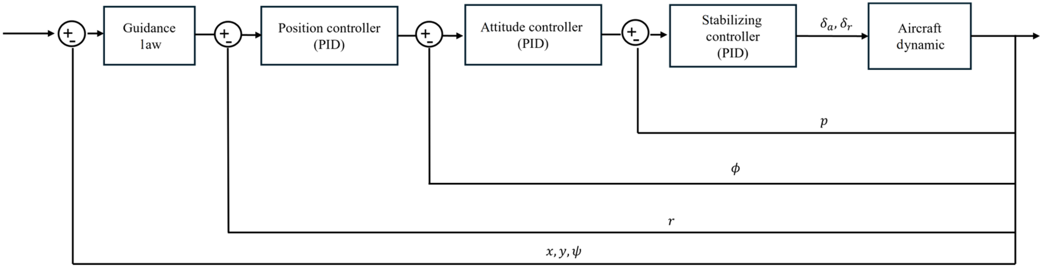
Integrating the guidance law and controller enables the aircraft to be guided onto the glide slope and localizer, even if it deviates from the runway.

2. Related Works

In the field of UAVs, there are different detection methods based on environmental differences. Traditional computer vision algorithms include the most common techniques such as color detection, morphology, Region of Interest (ROI), etc. A previous study [10] identified potential objects of interest in the image based on color and used filters such as erosion, dilation, and Gaussian blur to find the target pixels for ground target tracking. Line detection methods are not only used for runway detection but also lane tracking in autonomous driving [11] and horizon tracking [5]. Hough transform and random sample consensus (RANSAC) methods are used to compare the detection results of the two runway edges during landing. As the complexity of the environment increases, deep learning-based target detection methods have also been applied to UAVs. A previous study [12] enhanced the YOLOv5 architecture by incorporating geometric feature corner prediction methods into the model to conduct carrier landings. Beyond one-stage algorithms, two-stage algorithms first obtain bounding boxes of objects and then perform mask prediction on the pixels within the box. In another study [13], Mask-RCNN was utilized to extract segmentation contours and then to detect lines, which is more effective than traditional line detection methods. However, the drawback is its high computational resource consumption, making it challenging to apply in real-time environments.
By obtaining object information through the previously mentioned object detection methods, a monocular camera can solve the relative coordinate positions of the UAV’s attitude and object information. In this context, multirotors often use ArUco marker [14] and Helipad [15] to determine the pose of the landmark itself and then calculate the camera’s position in space. However, this method is not feasible for runway landings due to its inability to identify markers for positioning. Therefore, other studies [16,17] proposed the Plücker method, which involves detecting runway lines, calculating their slopes, and determining the aircraft’s longitudinal displacement, lateral displacement, and altitude relative to the runway. This method is more suitable for situations where the complete runway contour is clearly visible at close range. However, it has limitations because the longitudinal displacement is sensitive to the runway’s bottom edge lines, leading to inaccurate estimates. Therefore, another study [18] proposed a CNN regression model to replace the longitudinal displacement and compared the contour positioning solutions of different detection methods. In addition, the pinhole model and Perspective-n-Point (PnP) were used for camera optical positioning and solving positions [19]. In recent studies, deep learning models have been used to directly train estimated displacements, angles, and other parameters without considering complex calculations. One study [20] employed end-to-end learning to train the UAV’s relative heading angle to the runway in case of sensor failure. However, due to insufficient data collection, the fixed-wing UAV became uncontrollable during the final approach. In our previous work [18], cropped images were used to detect an approaching intruder by YOLOv3, and a CNN regression model was applied to determine the target UAV’s distance. Although many studies have proposed various positioning solutions, most experimental methods are based on simulated videos, with fewer utilizing optical positioning solutions or deep learning to estimate distances and provide guidance for UAV flight.
In addition, vision-based feedback control methods, including visual servoing [21], are commonly applied to multirotor UAVs. Visual servoing methods [21] include Position-Based Visual Servoing (PBVS) and Image-Based Visual Servoing (IBVS) [22]. PBVS uses vision to determine the three-axis position relative to the target as the input for the controller, while IBVS directly provides the controller with features extracted from the image. Both methods are commonly applied in multirotor UAVs and robotic arms. The study in [23] utilized IBVS, employing three visual features and desired features as errors to enable the aircraft to land on an aircraft carrier. Another study [24] also applied IBVS to design control laws for a monocular gimbal camera and to keep the object centered in the image while achieving effective tracking under different path-following scenarios.
Since fixed-wing UAVs require a predefined path to follow the glide slope during automatic landing, a further study [25] proposed a Line-of-Sight (LOS)-based longitudinal and lateral guidance law combined with an L1 controller to achieve automatic landing. Another study [26] presented the L1 guidance law, focusing on lateral maneuvers to enable fixed-wing UAVs to follow straight and circular paths. A study [27] discussed various longitudinal control landing systems for aircraft and implemented them in simulations. Another study [28] utilized visual positioning to determine runway distance and direction, which was combined with a PID controller, and the approach was validated using actual flight data.

3. System Overview

In this section, we introduce the research workflow, which is broadly divided into runway detection, distance estimation methods, image processing methods, and path following.

3.1. Research Overview

In this study, two deep learning models were mainly used as the approach for the runway visual landing system. To achieve real-time vision-based navigation in the simulation environment, a lightweight model of YOLOv8 was utilized for runway detection and localization. After detecting the runway, a CNN regression model was applied to determine the runway’s longitudinal distance, lateral distance, and glide slope angle. Image processing methods were applied to determine the angles of the two runway edge lines, providing a reference for checking whether the aircraft was aligned with the runway centerline. After obtaining the navigation information from image estimation, a low-pass filter was used to remove noise, and a guidance law was introduced to guide the aircraft along the desired glide path, whether it was directly aligned with or deviated from the runway. This system was implemented in the simulation environment X-Plane 11. Figure 1 shows the flowchart of this study, which includes runway detection, localization, line detection, and controller design.

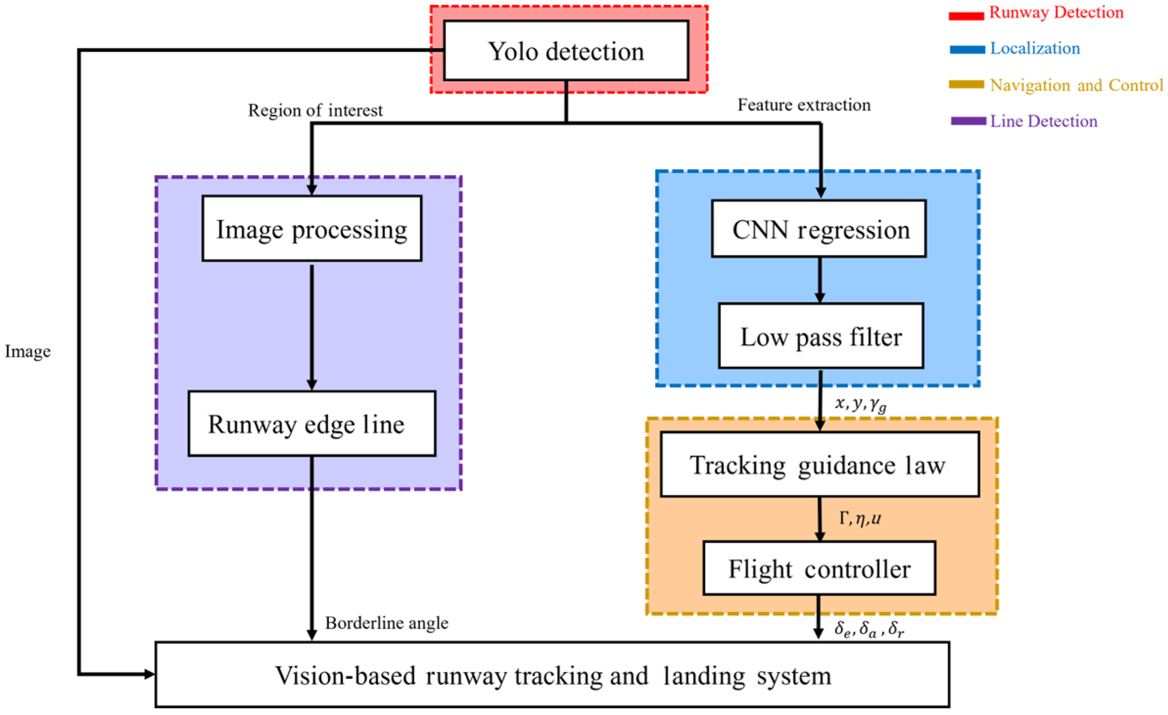
3.2. Architecture of Runway Detection and Tracking System

The system operation flowchart for runway detection and tracking is shown in Figure 2. When a fixed-wing aircraft is able to view the runway, a deep learning model is used to detect the runway instead of simply searching the entire image using image processing methods. A 200 × 200 pixel area extending outward from the bounding box center is used as a reference for estimating the runway distance and glide slope. Due to the regression model having a lateral deviation in specific scenarios, such as when aligning with the runway’s centerline, additional image processing methods are used within the bounding box to obtain the runway edges and correct the lateral estimation results. Finally, for the guidance law, both glide slope guidance and the L1 guidance law are simultaneously employed to direct the fixed-wing aircraft along the glide path. The control surface commands are then calculated using a cascaded control architecture.

4. Runway Detection and Localization

The YOLOv8 model is utilized to identify specific targets in complex terrains. The bounding box images are treated as regions of interest, whereas traditional image processing algorithms in OpenCV are combined to extract the required features. Deep learning models can be applied not only for object detection but also for classification and regression tasks. A CNN regression model is used to generate reference values to obtain control commands from images.

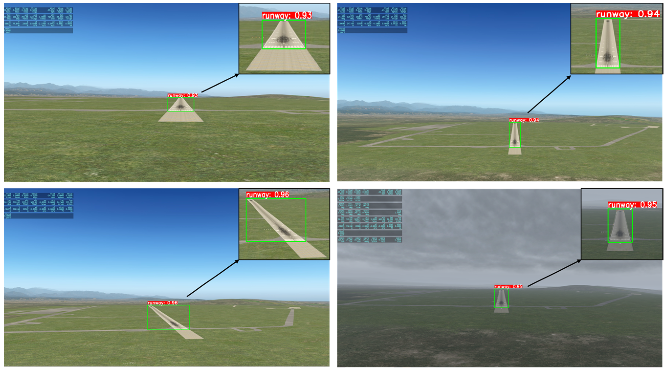
4.1. Real-Time Detection-YOLOv8

YOLOv8 [29] is developed by Ultralytics, continues the features of the YOLO architecture, and consists of three components. The backbone uses C2f to extract features and employs residual connections and bottleneck structures to reduce network size. The neck utilizes multi-scale feature fusion, enhancing the performance by combining feature maps from different stages of the backbone. The head is responsible for the final tasks of object detection and classification.
To ensure that the runway is detectable from various approach angles, a runway dataset for model training is needed. Approximately 13,000 images were collected by utilizing X-Plane 11 Flight Simulator, including approaching, crossing, and landing scenarios. The selected airport was Taichung International Airport, Taichung, Taiwan, which has the same configuration as the real airport. The model was trained for 100 epochs with an image size of 640 × 640 and a learning rate of 0.001. The dataset was split into training and validation sets in a 7:3 ratio for training and testing. The GPU used in this study for training the YOLOv8 model was an Nvidia GeForce RTX 4060Ti, and the training process took approximately 5 h.
Based on the requirements of training the subsequent CNN regression model to verify the model’s usability, the validation set of images in the dataset was used for evaluation. The validation formulas are shown in Equations (1) and (2). The precision value was 100%, and the recall was 99.8%. Figure 3 shows the runway detection results under different initial positions. These results will be used for further applications of image processing methods and regression model training.
P r e c i s i o n = T P T P + F P × 100 %
R e c a l l = T P T P + F N × 100 %
For insights on the performance of various deep learning algorithms for runway detection, refer to study [30]. This study compared several deep learning algorithms with different runway datasets, including Mask R-CNN and YOLOv8-seg. It incorporated diverse terrains, lighting, texture, and weather conditions, including images from the X-Plane 11 Flight Simulator, for performance and inference comparisons. In terms of average precision, the performance metrics show an AP50 of 80.7% for Mask R-CNN and 89.8% for YOLOv8-seg [30].

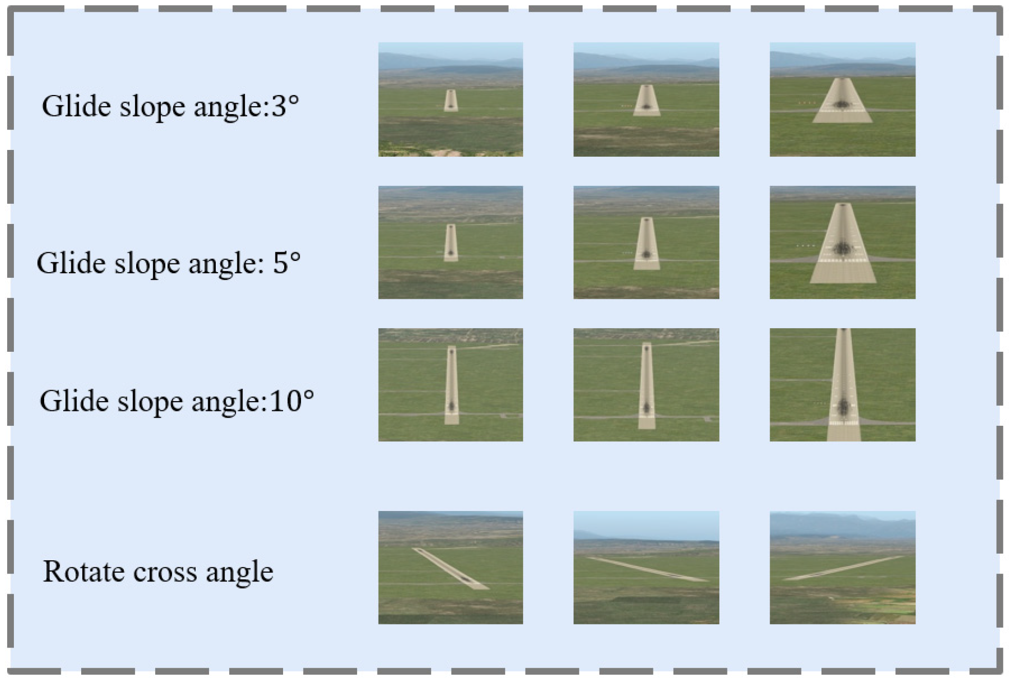
4.2. CNN Regression Model for Distance Estimation

In this section, an end-to-end training approach will be applied, using images as inputs and producing the reference commands required by the controller. The training method in study [18] was utilized, which involves collecting the required dataset using bounding box information.
Based on the concepts of the ILS’s glide slope and localizer, additional datasets are needed to train the regression model to obtain the distance to the runway from different angles. By collecting data from specified locations in X-Plane 11, a total of approximately 15,000 images were gathered. Using the trained YOLOv8 model, a 200 × 200 pixel area extending outward from the bounding box center was used as the dataset. The data collection method involved calculating the deviation angle to determine specific position points and obtaining the aircraft’s relative distance to the runway for annotation. The information on data collection is shown in Table 1. The applicable range of this study enables effective runway distance and angle estimation within a 10-degree lateral deviation and a 10-degree longitudinal deviation from the runway. Figure 4 shows the cropped images from different angles.
The backbone model adopted in this study is the VGG16 model. The pre-trained weights used are from ImageNet for subsequent transfer learning applications. As shown in Figure 5, the architecture of the regression network consists of three fully connected layers. The output value provides the required longitudinal distance, lateral distance, and glide slope angle.

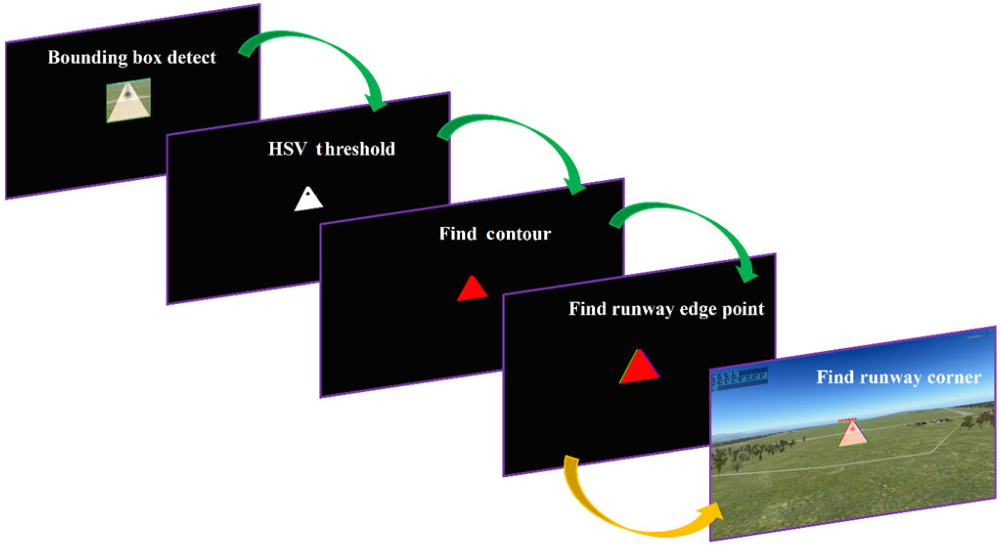
4.3. Image Processing for Runway Centerline Detection

To reduce the oscillation and steady state error of lateral control in tracking the runway centerline, a runway centerline detection method was developed based on image processing to determine two angles of runway edges. According to the previous literature, various methods for detecting runway boundaries have been discussed, and it has been suggested that the contours obtained from segmentation can be corrected using traditional image processing techniques to address the jagged edge issue [18]. Therefore, this study is inspired by the concept of two-stage detection methods. First, the threshold of the HSV (Hue, Saturation, Value) color model is used to find the values close to the runway surface. Then, morphological operations are conducted to address the missing black areas in the runway landing zone. After roughly identifying the runway contours, Convex Hull is used to locate the outermost points of the current contour, and using linear regression, namely the least squares method, the polynomial functions for the left and right lines are obtained. This process allows for identification of the four corner points of the runway and fitting the runway lines. Figure 6 illustrates the complete image processing procedure.
According to study [31], when a + b > t h r e s h o l d , the UAV is on the left side of the runway; when a + b < t h r e s h o l d , the UAV is on the right side of the runway; and when a + b = 0 , the UAV is on the centerline of the runway. By calculating the sum of the angles, if the regression model’s predicted lateral displacement does not match this calculation, a correction will be made to bring the UAV back to the runway centerline. The threshold is set between 0 and 1, as illustrated in Figure 7.

5. Runway Tracking and Automatic Landing Control

This section describes the use of a predefined path to guide the aircraft to the glide slope path for landing, including longitudinal control and lateral control, with the runway threshold set as the target landing point.

5.1. System Coordinate Definition

The OpenGL coordinate system used in the X-Plane 11 simulation environment has the positive X-axis pointing east, the positive Y-axis pointing up, and the positive Z-axis pointing south. Since this coordinate system is inconvenient for aircraft navigation systems, it needs to be converted to the more commonly used NED (North-East-Down) coordinate system for UAVs. This study uses a 2D coordinate system rotation. The angle is calculated using the straight line formed by the start and end points of the runway, with the runway threshold set as the origin of the local coordinate system. The altitude is adjusted by translating it to obtain the relative height of the runway, as shown in Figure 8.

5.2. Glide Slope for Longitudinal Control

During the glide phase of the landing process, glide slope guidance can provide the aircraft with distance error relative to the runway [27]. When the aircraft deviates from the glide slope, there is a vertical distance, d , between the aircraft’s center of gravity and the glide slope. By knowing the aircraft’s forward speed and flight path angle, the change of the deviation from the glide slope, d ˙ , can be determined. The hypotenuse distance of the glide slope, R , can be calculated from the aircraft’s longitudinal distance and altitude. These values yield the aircraft’s current deviation angle, Γ , from the glide slope, with the objective being to eliminate the deviation error, as shown in Figure 9.
The definitions of altitude and slant distance are as follows
h = x tan γ g
R = x 2 + h 2
where γ g is the glide slope angle predicted by the image, and x is the longitudinal distance value estimated by the image. The formula for calculating the distance error between the aircraft and the glide slope is as follows:
d ˙ = V sin γ v V 57.3 γ v   ( r a d i a n s )
Γ = d R   ( d e g r e e s )
where γ v = γ + γ g , and Γ represents the glide slope angle deviation.
By setting the reference path angle and the path deviation angle, the error can be input into the position controller, referred to as the Glide Path Coupled controller. A PID controller is used, and the error obtained from this controller is then passed to the autopilot’s attitude controller and stability augmentation controller to determine the elevator command angle. The longitudinal control architecture is shown in Figure 10.
The aircraft’s forward speed is controlled through throttle adjustments. In this study, the throttle ratio is modified to achieve constant speed control during automatic landing. The designed control loop adopts a PID controller to calculate the error between the reference and current speeds and then proportionally adjusts the throttle to maintain the desired speed [28].

5.3. Runway Centerline Tracking for Lateral Control

In addition to longitudinal landing control, ensuring that the aircraft can stably fly along the runway centerline is crucial. The path-following guidance law in study [26] is adopted, which enables fixed-wing aircraft to follow a straight flight path. The reference points on the path are determined by the L1 distance. A circle with a radius equal to the L1 distance is drawn with the UAV’s position as the origin. This circle intersects the linear equation at two reference points, and the point closest to the UAV’s heading is designated as the target point, as shown in Figure 11.
where ( x u a v , y u a v ) , ( x p , y p ) L 1 , ψ are the UAV’s longitudinal distance and lateral distance predicted by image, target point, look-ahead distance, and heading. This study uses a two-dimensional linear equation as the predefined path. Centripetal acceleration is also considered to determine the limitation of the UAV’s turning radius. Here, η represents the angle between the L1 distance and the UAV’s heading:
a c = 2 u 2 L 1 sin η
where a c and u are centripetal acceleration and UAV’s forward speed, respectively. The heading angle deviation is calculated using centripetal acceleration. The heading angle deviation is calculated using centripetal acceleration, defined as:
Δ ψ = a c u   Δ t
where t is the time step, and then the yawing rate command is as follows:
r c = Δ ψ Δ t = a c u
In this study, the yawing rate is used in place of the heading angle deviation for the outer loop control method. A PID controller is employed, and the resulting aileron control command is derived from the inner loop. Additionally, the calculated aileron command is proportionally applied to the rudder. The lateral control architecture is shown in Figure 12.

6. Automatic Landing Simulations and Results

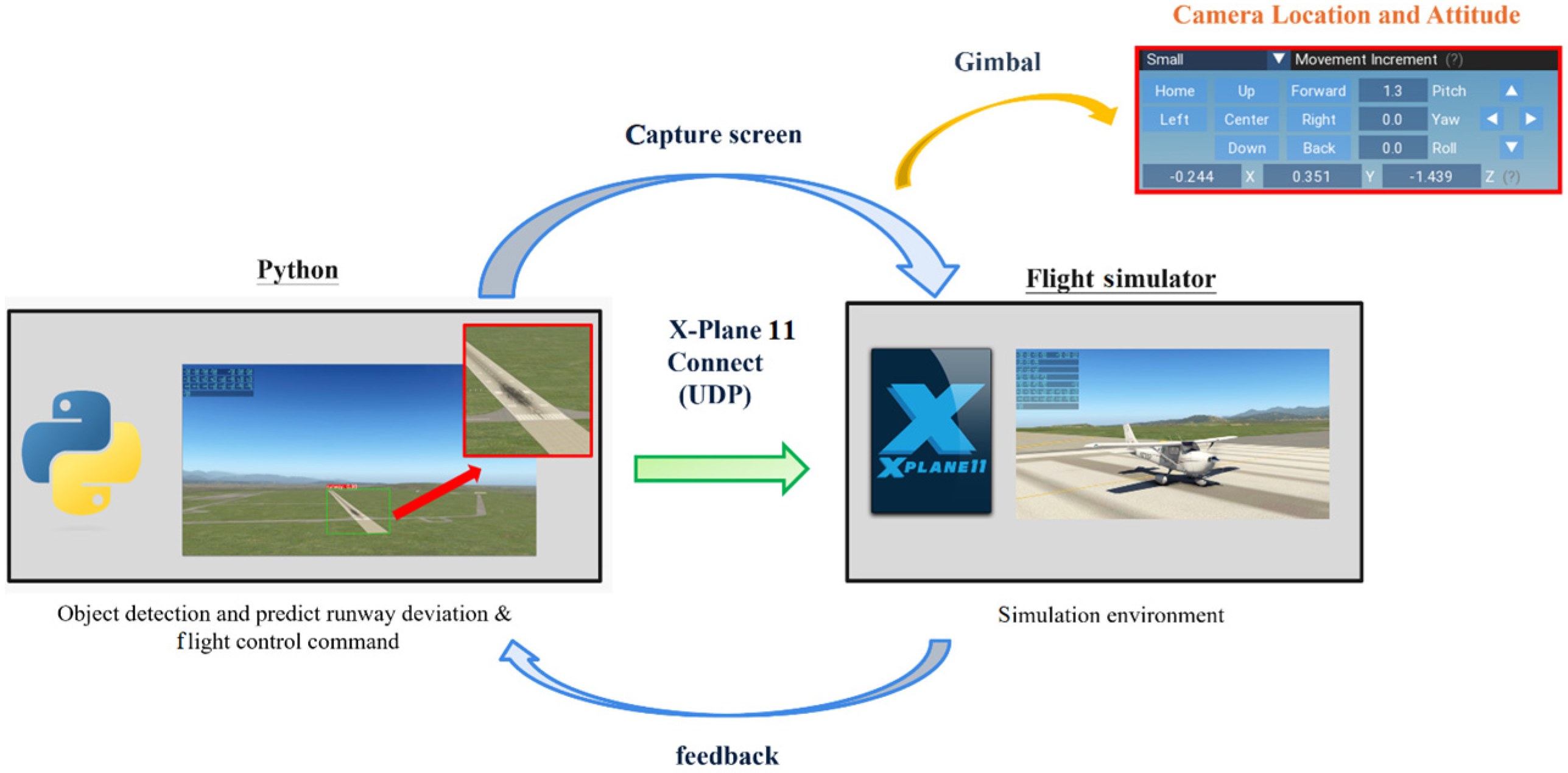
6.1. Simulation Environment Setup

X-Plane 11 Flight Simulator was adopted in this study as the simulation environment, and the aircraft chosen for the simulation was the Cessna 172 Skyhawk, representing a fixed-wing UAV. The X-Plane 11 Connect Toolbox was employed to send control commands via UDP to control the aircraft. Figure 13 shows the real-time system software-in-the-loop simulation. To prevent image instability caused by aircraft movements, a gimbal system was used to keep the camera level and stable. The simulations were conducted at the recommended landing speed of 45 m/s for Cessna 172 aircraft.

6.2. Simulation Cases

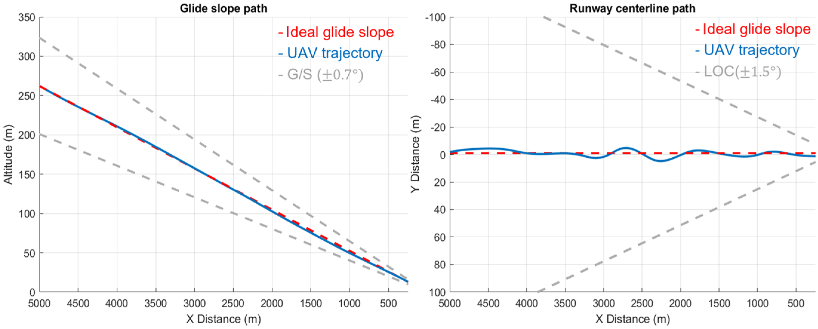
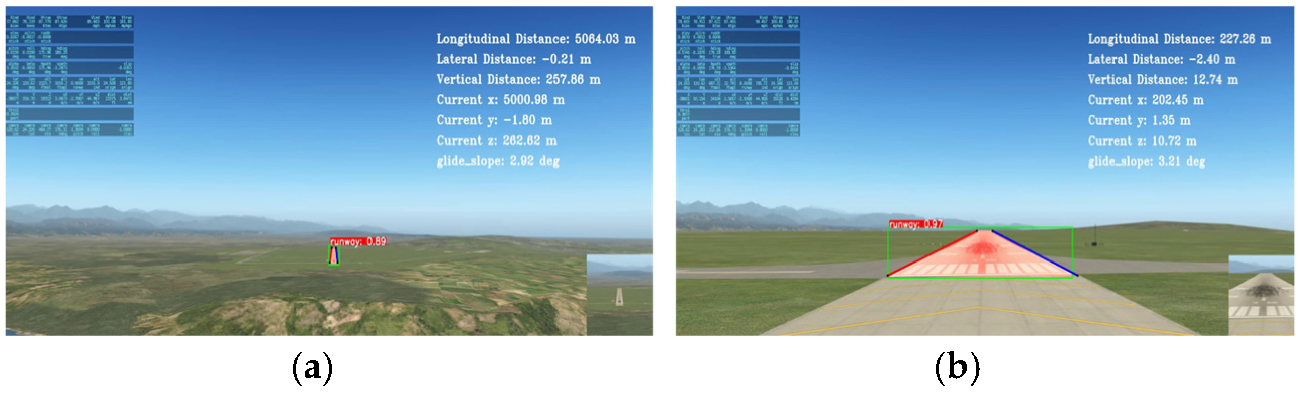
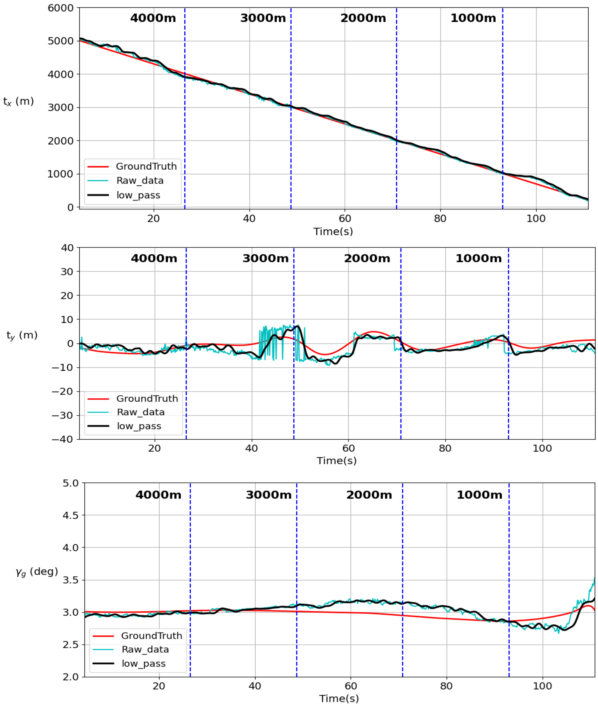
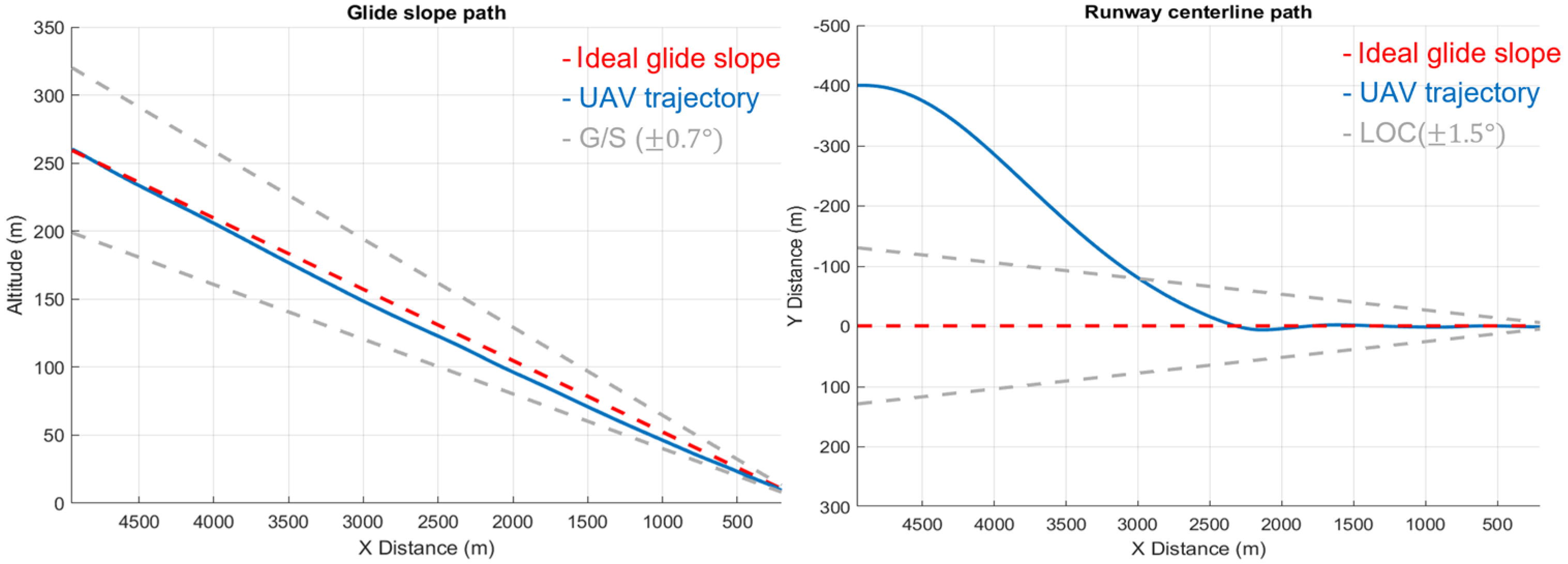
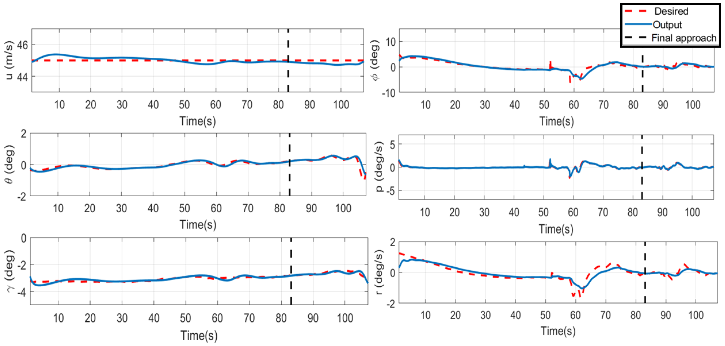
6.2.1. Case 1: 5 Km and 3° Glide Slope Landing

Case 1 describes a scenario where the aircraft is directly facing the runway, starting from 5 km. The image detection and regression model information are used as guidance for the UAV to perform a 3-degree glide slope landing. Figure 14 shows the longitudinal and lateral tracking results. To observe whether the flight trajectory falls within the recommended ILS range, this study uses a glide slope (G/S) tolerance of ± 0.7 degrees and a localizer (LOC) tolerance of ± 1.5 degrees as the target ranges.
The longitudinal tracking results of the 3-degree glide slope are effective, as the image accurately predicts the runway under these conditions. In the lateral tracking results, the larger deviations are caused by the regression model predicting higher values. By using the angle determination mechanism, the system can identify which side of the runway the aircraft is located on. It allows for quick corrections by issuing control commands to the aircraft. Figure 15 shows the responses of longitudinal and lateral control. Figure 16 illustrates the detection results of different distances away from the target runway in Case 1. Figure 17 shows the estimation results compared to the ground truth.
In Figure 17, it can be observed that the lateral deviations from the desired glide slope have significant fluctuations. This is due to the results of line segment detection. To address the regression model’s tendency to generate positive or negative distance errors when oriented directly toward the runway, this study utilizes a line detection method to correct the runway alignment by artificially providing the model with the opposite result. The low pass filter is then applied to prevent the controller from tracking these disturbances, which would otherwise cause the UAV to undergo severe oscillations. Multiple experimental results indicate that if the lateral distance error is less than 10 m, the UAV can align more accurately with the runway centerline.

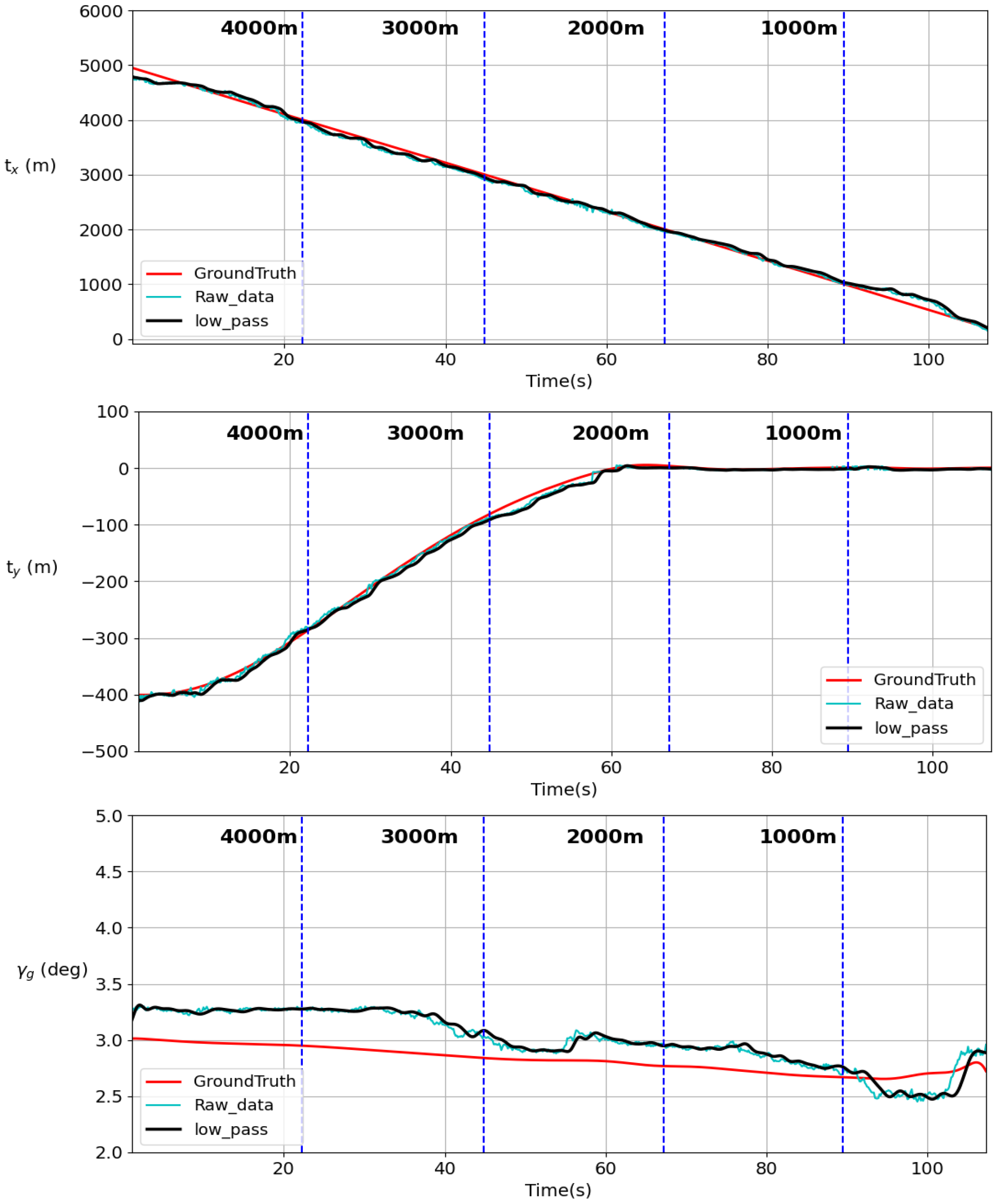
6.2.2. Case 2: Left Cross with 5° Path

In Case 2, the UAV starts at 5 km distance with a lateral deviation of 400 m, which has a heading error of 5 degrees away from the runway’s centerline. The UAV’s heading is aligned with the runway direction, performing a 3-degree glide slope landing while simultaneously aligning with the runway. In this scenario, the UAV must perform minimal rolling maneuvers to align with the runway, avoiding situations where attitude control could cause the camera to lose sight of the runway. Therefore, the reference point distance for the guidance law will gradually decrease based on the predicted lateral distance, starting from 1300 m and reducing to 200 m. Figure 18 shows the longitudinal and lateral tracking results. In the longitudinal tracking, if the initially estimated glide slope angle is too large, it will cause deviations; however, as the altitude decreases, the glide slope eventually corrects back to the 3-degree path. In the lateral tracking, the UAV returns to the runway centerline when it is approximately 2000 m from the runway. The responses of the longitudinal and lateral control are shown in Figure 19.
Figure 20 shows the estimated results compared to the ground truth. It illustrates the detection and localization when the aircraft performs the landing in Case 2. The angle determination mechanism activates once the UAV aligns with the runway, as illustrated in Figure 21. With a significant lateral deviation, the angles of the runway edges differ significantly from those in a straight approach scenario. The left edge angle is greater than the right edge angle. During this period, the predicted lateral distance is sufficient to determine which side of the runway the UAV is on.

6.2.3. Case 3: 2 Km and 5° Glide Slope Landing

In Case 3, a glide slope landing is conducted with the UAV directly facing the runway and aligned with the runway centerline, assessing whether a 3-degree glide slope can be applied for landing at greater angles. This evaluates the ability of the regression model to accurately predict positions with different runway profiles at closer ranges. Figure 22 shows the longitudinal and lateral tracking results. In the longitudinal tracking, it can be observed that flight path errors are more significant than the errors in Case 2. Although the aircraft deviates from the glide path in this scenario, the trend eventually slowly returns to the 5-degree glide path. Figure 23 shows the responses of the automatic landing system. Figure 24 shows the estimation results compared to the ground truth.
Table 2, Table 3 and Table 4 present the root mean square error (RMSE) between the predicted results from the CNN regression model and the ground truth across various simulation scenarios. The vertical distances are calculated based on the longitudinal distance and glide slope angle. In Case 1, the CNN regression model effectively predicted longitudinal distance, lateral distance, and glide slope angle. As indicated in Table 2, the root mean square error (RMSE) for longitudinal distance is generally below 100 m, except for the range between 1000 and 200 m. The longitudinal errors in the CNN predictions between 1000 and 200 m are larger than those at high altitudes. This is because the adopted dataset for distance estimation for long-range detection, ranging from 5500 to 0 m, is created using images that are 200 × 200 pixels, extending outward from the center of the bounding box. However, when the aircraft approaches the runway, the bounding box may exceed 200 × 200 pixels, leading to an increase in longitudinal error during low-altitude scenarios. However, the glide path guidance calculation primarily focuses on the glide slope angle calculations, so as long as the distance errors are not significantly large, a successful landing can be achieved. A successful landing can be achieved when the glide slope estimation is sufficiently accurate.
In Case 2, the results reveal that the longitudinal distance error is comparable to that in Case 1; however, the lateral errors are greater due to a more significant deviation from the runway’s centerline at the start of the approach. In Case 3, the predicted glide slope angles perform worse than in the previous two cases. As shown in Table 4, the maximum deviation between 2500 m and 1500 m exceeds 0.5 degrees, which negatively impacts the precision of following the glide path. Consequently, as illustrated in Figure 24, the UAV deviates from the intended 5-degree glide slope and descends at a steeper angle. Fortunately, during the final approach, the regression model predicted a glide slope that was already below 5 degrees, enabling the UAV to correct its trajectory and return to the ideal glide path.

6.3. Simulation Result Discussion

Table 5 presents the errors between the UAV’s flight trajectory and the ideal glide slope trajectory. From the simulation results, it can be observed that the measurements of all cases below the decision height, the altitude of 200 ft, meet the required standards of the ILS glide slope and localizer, which are the errors within 17 m in horizontal and 10 m in vertical estimations. However, the estimation of longitudinal distance is noticeably lower. Despite multiple adjustments to the model during training, achieving accurate estimates in this scenario remains challenging, likely due to the method of dataset collection. Based on the longitudinal tracking results for each simulation scenario, in each case, the RMSE is less than 10 m. Case 1, which involves a 3-degree glide slope directly facing the runway, has the best tracking performance.
In this study, two deep learning methods were adopted to detect the runway and estimate guidance information. Glide slope guidance and L1 guidance laws were used to determine control commands in longitudinal and lateral motions. Through validation in a simulated environment, the system successfully performed real-time automatic landing and alignment with the runway, relying on image information in a GNSS-denied environment.
The runway detection results show that both the YOLOv8 model and the line detection method achieved a 100% accuracy rate. Compared with the correction mechanism using Hough transform, the regression line method using the least squares approach is more robust. From the real-time runway detection, guidance, and control validation in simulations, the proposed automatic landing approach in a GNSS-denied environment was successfully executed in all simulation cases. With the glide slope guidance algorithm, it was found that among the three estimated image solutions, the glide slope angle was the most critical. This value was directly inputted into the UAV’s flight path angle to eliminate errors. While the aircraft’s relative position to the runway was also needed, as long as the distance error was not too significant, the glide slope angle could correct the path to the glide slope. The adopted L1 guidance law, as a method for path following, is also suitable for maintaining alignment with the runway centerline. In straight approach scenarios, edge detection helps ensure that even if the regression model makes a prediction error, the system can quickly correct the aircraft back to the runway centerline.

7. Conclusions

In this study, a vision-based automatic landing system using a monocular camera in a GPS-denied environment is proposed to compose an alternative navigation system based on deep learning methods. By integrating the localization solution into flight control and guidance laws, a complete real-time automatic landing system was demonstrated in the simulation environment with the help of deep learning methods, YOLOv8, and CNN regression. Without relying on optical positioning methods, such as the pinhole model and PnP, runway localization is achieved through deep learning in a GNSS-denied environment. It addresses the issue of jagged contours commonly found in traditional methods and other deep learning models by implementing a robust line detection technique. The study utilizes glide slope guidance and path-following methods to calculate aircraft guidance laws, allowing the aircraft to track the glide path effectively. Moreover, the cascade control system can incorporate traditional PID controllers for vision-based guidance. The simulation results indicate that glide path guidance and landing can be successfully achieved from various initial positions in a simulated environment. The dataset used in this study can perform vision-based navigation and guidance for fixed-wing aircraft within the range of glide slopes (2°~10°) and cross angles (−10°~10°). Finally, whether following a 3-degree or 5-degree glide slope, the UAV’s flight trajectory remained within the glide slope ± 0.7 degrees and localizer ± 1.5 degrees, with the tracking error consistently less than 10 m.

Author Contributions

Conceptualization, Y.-X.L. and Y.-C.L.; methodology, Y.-X.L. and Y.-C.L.; software, Y.-X.L.; validation, Y.-X.L. and Y.-C.L.; formal analysis, Y.-X.L.; investigation, Y.-X.L.; resources, Y.-C.L.; data curation, Y.-X.L.; writing—original draft preparation, Y.-X.L.; writing—review and editing, Y.-X.L. and Y.-C.L.; visualization, Y.-X.L. and Y.-C.L.; supervision, Y.-C.L.; project administration, Y.-C.L.; funding acquisition, Y.-C.L. All authors have read and agreed to the published version of the manuscript.

Funding

This research was funded by the National Science and Technology Council (NSTC) under grant numbers NSTC 113-2218-E-006-004- and NSTC 112-2221-E-006-105-MY3.

Institutional Review Board Statement

Not applicable.

Informed Consent Statement

Not applicable.

Data Availability Statement

The raw data supporting the conclusions of this article will be made available by the authors on request.

Conflicts of Interest

The authors declare no conflicts of interest.

References

  1. Balduzzi, G.; Ferrari Bravo, M.; Chernova, A.; Cruceru, C.; van Dijk, L.; de Lange, P.; Jerez, J.; Koehler, N.; Koerner, M.; Perret-Gentil, C. Neural Network Based Runway Landing Guidance for General Aviation Autoland; Department of Transportation, Federal Aviation Administration: Washington, DC, USA, 2021. [Google Scholar]
  2. Watanabe, Y.; Manecy, A.; Amiez, A.; Aoki, S.; Nagai, S. Fault-tolerant final approach navigation for a fixed-wing uav by using long-range stereo camera system. In Proceedings of the 2020 International Conference on Unmanned Aircraft Systems (ICUAS), Athens, Greece, 1–4 September 2020; IEEE: Piscataway, NJ, USA, 2020; pp. 1065–1074. [Google Scholar]
  3. Zhang, L.; Zhai, Z.; He, L.; Niu, W. Infrared-based autonomous navigation for civil aircraft precision approach and landing. IEEE Access 2019, 7, 28684–28695. [Google Scholar] [CrossRef]
  4. Kong, W.; Zhou, D.; Zhang, Y.; Zhang, D.; Wang, X.; Zhao, B.; Yan, C.; Shen, L.; Zhang, J. A ground-based optical system for autonomous landing of a fixed wing uav. In Proceedings of the 2014 IEEE/RSJ International Conference on Intelligent Robots and Systems, Chicago, IL, USA, 14–18 September 2014; IEEE: Piscataway, NJ, USA, 2014; pp. 4797–4804. [Google Scholar]
  5. Tripathi, A.K.; Patel, V.V.; Padhi, R. Vision based automatic landing with runway identification and tracking. In Proceedings of the 2018 15th International Conference on Control, Automation, Robotics and Vision (ICARCV), Singapore, 18–21 November 2018; IEEE: Piscataway, NJ, USA, 2018; pp. 1442–1447. [Google Scholar]
  6. Wang, Z.; Zhao, D.; Cao, Y. Visual navigation algorithm for night landing of fixed-wing unmanned aerial vehicle. Aerospace 2022, 9, 615. [Google Scholar] [CrossRef]
  7. He, K.; Gkioxari, G.; Dollár, P.; Girshick, R. Mask r-cnn. In Proceedings of the IEEE International Conference on Computer Vision, Venice, Italy, 22–29 October 2017; pp. 2961–2969. [Google Scholar]
  8. Terven, J.; Cordova-Esparza, D. A comprehensive review of yolo: From yolov1 to yolov8 and beyond. arXiv 2023, arXiv:2304.00501. [Google Scholar]
  9. Bolya, D.; Zhou, C.; Xiao, F.; Lee, Y.J. Yolact: Real-time instance segmentation. In Proceedings of the IEEE/CVF International Conference on Computer Vision, Seoul, Republic of Korea, 27 October–2 November 2019; pp. 9157–9166. [Google Scholar]
  10. Wang, X.; Zhu, H.; Zhang, D.; Zhou, D.; Wang, X. Vision-based detection and tracking of a mobile ground target using a fixed-wing uav. Int. J. Adv. Robot. Syst. 2014, 11, 156. [Google Scholar] [CrossRef]
  11. Miyamoto, R.; Nakamura, Y.; Adachi, M.; Nakajima, T.; Ishida, H.; Kojima, K.; Aoki, R.; Oki, T.; Kobayashi, S. Vision-based road-following using results of semantic segmentation for autonomous navigation. In Proceedings of the 2019 IEEE 9th International Conference on Consumer Electronics (ICCE-Berlin), Berlin, Germany, 8–11 September 2019; IEEE: Piscataway, NJ, USA, 2019; pp. 174–179. [Google Scholar]
  12. Ma, N.; Weng, X.; Cao, Y.; Wu, L. Monocular-vision-based precise runway detection applied to state estimation for carrier-based uav landing. Sensors 2022, 22, 8385. [Google Scholar] [CrossRef] [PubMed]
  13. Akbar, J.; Shahzad, M.; Malik, M.I.; Ul-Hasan, A.; Shafait, F. Runway detection and localization in aerial images using deep learning. In Proceedings of the 2019 Digital Image Computing: Techniques and Applications (DICTA), Perth, Australia, 2–4 December 2019; IEEE: Piscataway, NJ, USA, 2019; pp. 1–8. [Google Scholar]
  14. Bhargavapuri, M.; Shastry, A.K.; Sinha, H.; Sahoo, S.R.; Kothari, M. Vision-based autonomous tracking and landing of a fully-actuated rotorcraft. Control Eng. Pract. 2019, 89, 113–129. [Google Scholar] [CrossRef]
  15. Chen, C.; Chen, S.; Hu, G.; Chen, B.; Chen, P.; Su, K. An auto-landing strategy based on pan-tilt based visual servoing for unmanned aerial vehicle in gnss-denied environments. Aerosp. Sci. Technol. 2021, 116, 106891. [Google Scholar] [CrossRef]
  16. Wolkow, S.; Schwithal, A.; Tonhäuser, C.; Angermann, M.; Hecker, P. Image-aided position estimation based on line correspondences during automatic landing approach. In Proceedings of the ION 2015 Pacific PNT Meeting, Honolulu, HI, USA, 20–23 April 2015; pp. 702–712. [Google Scholar]
  17. Wolkow, S.; Schwithal, A.; Angermann, M.; Dekiert, A.; Bestmann, U. Accuracy and availability of an optical positioning system for aircraft landing. In Proceedings of the 2019 International Technical Meeting of the Institute of Navigation, Reston, VA, USA, 28–31 January 2019; pp. 884–895. [Google Scholar]
  18. Lai, Y.-C.; Huang, Z.-Y. Detection of a moving uav based on deep learning-based distance estimation. Remote Sens. 2020, 12, 3035. [Google Scholar] [CrossRef]
  19. Ruchanurucks, M.; Rakprayoon, P.; Kongkaew, S. Automatic landing assist system using imu+ p n p for robust positioning of fixed-wing uavs. J. Intell. Robot. Syst. 2018, 90, 189–199. [Google Scholar] [CrossRef]
  20. Bicer, Y.; Moghadam, M.; Sahin, C.; Eroglu, B.; Üre, N.K. Vision-based uav guidance for autonomous landing with deep neural networks. In Proceedings of the AIAA Scitech 2019 Forum, San Diego, CA, USA, 7–11 January 2019; p. 0140. [Google Scholar]
  21. Chaumette, F.; Hutchinson, S. Visual servo control. I. Basic approaches. IEEE Robot. Autom. Mag. 2006, 13, 82–90. [Google Scholar] [CrossRef]
  22. Machkour, Z.; Ortiz-Arroyo, D.; Durdevic, P. Classical and deep learning based visual servoing systems: A survey on state of the art. J. Intell. Robot. Syst. 2022, 104, 11. [Google Scholar] [CrossRef]
  23. Coutard, L.; Chaumette, F.; Pflimlin, J.-M. Automatic landing on aircraft carrier by visual servoing. In Proceedings of the 2011 IEEE/RSJ International Conference on Intelligent Robots and Systems, San Francisco, CA, USA, 25–30 September 2011; IEEE: Piscataway, NJ, USA, 2011; pp. 2843–2848. [Google Scholar]
  24. Yang, L.; Liu, Z.; Wang, X.; Yu, X.; Wang, G.; Shen, L. Image-based visual servo tracking control of a ground moving target for a fixed-wing unmanned aerial vehicle. J. Intell. Robot. Syst. 2021, 102, 1–20. [Google Scholar] [CrossRef]
  25. You, D.I.; Jung, Y.D.; Cho, S.W.; Shin, H.M.; Lee, S.H.; Shim, D.H. A guidance and control law design for precision automatic take-off and landing of fixed-wing uavs. In Proceedings of the AIAA Guidance, Navigation, and Control Conference, Minneapolis, MN, USA, 13–16 August 2012; p. 4674. [Google Scholar]
  26. Park, S.; Deyst, J.; How, J. A new nonlinear guidance logic for trajectory tracking. In Proceedings of the AIAA Guidance, Navigation, and Control Conference and Exhibit, Providence, RI, USA, 16–19 August 2004; p. 4900. [Google Scholar]
  27. Lungu, R.; Lungu, M.; Grigorie, L.T. Alss with conventional and fuzzy controllers considering wind shear and gyro errors. J. Aerosp. Eng. 2013, 26, 794–813. [Google Scholar] [CrossRef]
  28. Shoouri, S.; Jalili, S.; Xu, J.; Gallagher, I.; Zhang, Y.; Wilhelm, J.; Jeannin, J.-B.; Ozay, N. Falsification of a vision-based automatic landing system. In Proceedings of the AIAA Scitech 2021 Forum, Virtual, 11–15 January 2021; p. 0998. [Google Scholar]
  29. Ultralytics YOLOv8. Available online: https://github.com/ultralytics/ultralytics (accessed on 27 February 2025).
  30. Wang, Q.; Feng, W.; Zhao, H.; Liu, B.; Lyu, S. Valnet: Vision-based autonomous landing with airport runway instance segmentation. Remote Sens. 2024, 16, 2161. [Google Scholar] [CrossRef]
  31. Shang, J.; Shi, Z. Vision-based runway recognition for uav autonomous landing. Int. J. Comput. Sci. Netw. Secur. 2007, 7, 112–117. [Google Scholar]
Figure 1. The architecture of a vision-based landing system.
Aerospace 12 00324 g001
Figure 2. Runway detection and localization process.
Aerospace 12 00324 g002
Figure 3. The detection results from different positions.
Aerospace 12 00324 g003
Figure 4. Cropped image with different positions.
Aerospace 12 00324 g004
Figure 5. The transfer learning of the regression network.
Aerospace 12 00324 g005
Figure 6. The process of runway line detection.
Aerospace 12 00324 g006
Figure 7. Runway centerline determination, where a and b are the left and right angles of runway edges.
Aerospace 12 00324 g007
Figure 8. The coordinate definition of the simulation environment.
Aerospace 12 00324 g008
Figure 9. The diagram of glide slope guidance.
Aerospace 12 00324 g009
Figure 10. Longitudinal control architecture.
Aerospace 12 00324 g010
Figure 11. The illustration of L1 guidance law.
Aerospace 12 00324 g011
Figure 12. Lateral control architecture.
Aerospace 12 00324 g012
Figure 13. Diagram of software in the loop process.
Aerospace 12 00324 g013
Figure 14. Glide slope path and centerline tracking results in Case 1.
Aerospace 12 00324 g014
Figure 15. Longitudinal and lateral responses in Case 1.
Aerospace 12 00324 g015
Figure 16. Detection results of different ranges (a) 5000 m (b) 200 m away from the target runway.
Aerospace 12 00324 g016
Figure 17. The estimated results compared to the ground truth in Case 1.
Aerospace 12 00324 g017
Figure 18. Glide slope path and centerline tracking results in Case 2.
Aerospace 12 00324 g018
Figure 19. Longitudinal and lateral responses in Case 2.
Aerospace 12 00324 g019
Figure 20. The estimated results compared to the ground truth in Case 2.
Aerospace 12 00324 g020
Figure 21. Runway edge angle detection results of Case 2.
Aerospace 12 00324 g021
Figure 22. Glide slope path and centerline tracking results in Case 3.
Aerospace 12 00324 g022
Figure 23. Longitudinal and lateral responses in Case 3.
Aerospace 12 00324 g023
Figure 24. The estimated results compared to the ground truth in Case 3.
Aerospace 12 00324 g024
Table 1. The training dataset of CNN regression.
Information on the Training Dataset
Image resolution1920 × 1080 (pixels)
Field of View (FOV)60 (deg)
Longitudinal distance0~5500 (m)
Lateral distance−900~900 (m)
Vertical distance0~900 (m)
Crossing angle−10~10 (deg)
Glide slope angle2~10 (deg)
Table 2. The RMSE of estimated displacements and glide slope in Case 1.
Distance (m)5000–30003000–10001000–2005000–200
Longitudinal (m)73.2145.88103.6269.93
Lateral (m)2.212.472.382.35
Vertical (m)3.597.884.165.85
Glide slope ( ° )0.0440.1480.1350.114
Table 3. The RMSE of estimated displacements and glide slope in Case 2.
Distance (m)5000–30003000–10001000–2005000–200
Longitudinal (m)74.8238.77122.0073.61
Lateral (m)7.458.281.927.24
Vertical (m)20.596.914.5514.10
Glide slope ( ° )0.3110.1650.1430.234
Table 4. The RMSE of estimated displacements and glide slope in Case 3.
Distance (m)2500–15001500–10001000–2002500–200
Longitudinal (m)66.4330.0397.7473.94
Lateral (m)3.093.743.583.42
Vertical (m)24.0210.126.4216.83
Glide slope ( ° )0.5220.3320.1790.390
Table 5. The errors of flight path compared to the ideal glide slope path cross-tracking error results.
Simulation Case Maximum Error (m)RMSE (m)
Case 13.19451.6585
Case 28.90856.3097
Case 39.48586.2791
Disclaimer/Publisher’s Note: The statements, opinions and data contained in all publications are solely those of the individual author(s) and contributor(s) and not of MDPI and/or the editor(s). MDPI and/or the editor(s) disclaim responsibility for any injury to people or property resulting from any ideas, methods, instructions or products referred to in the content.

