Dynamic Modeling of Aeroengine Rotor Speed Based on Data Fusion Method

Abstract

In this paper, a data-driven system identification method is presented based on the data fusion of a dynamic model and flight test data. The dynamic model is built by a combination of nonlinear auto-regressive networks (NARX) and the steady-state model. In such a combination, NARX can calibrate the dynamic characteristics of high-pressure and low-pressure rotor speed based on automatic control system steady-state models. As such, the calibrated engine model’s output speed is able to meet the requirements of simulation test tolerance accuracy. To enhance the robustness of the dynamic model against measurement noise, the Kalman filter is used to fuse the model prediction and the measurement data with noise. As such, the fused model can efficiently remove the influence of measurement noise and improve prediction accuracy. The proposed method supports the construction of reliable and environment-adaptive platforms for simulation application verification and provides high-fidelity simulation incentives for the realization of simulation test scenarios in the aviation industry.

1. Introduction

Recognition, state estimation, and control are three interrelated fields of modern automatic control system control theory. The support of recognition and state estimation is necessary in control theory; similarly, the application of control theory cannot proceed without recognition and state estimation techniques. Recently, modern control theory has become more and more applicable, and its practical consumption is not possible without utilizing a mathematical model of the control object. In most cases, the mathematical model of the work process of a controlled object is either unknown or does not comprehensively cover all the parameters of the process. Therefore, for an automatic control system control to solve practical problems, it is important to establish a proper mathematical model for the controlled object [1]. Recent advances in stochastic variational inference have enabled state estimation of systems with partially unknown dynamics, offering a Bayesian framework to handle model uncertainties [2].

For complex systems such as automatic control systems, classical identification is out of reach, but with the advent of computer science, a number of effective modern system identification methods have emerged recently, including the multi-layer recursive method [3], genetic algorithm identification [4,5], fuzzy logic method [6,7], and neural network method [8,9,10]. Notably, NARX neural networks have demonstrated superior performance in nonlinear time-series modeling, as evidenced by their application in structural deformation prediction and turbine dynamic characterization [11]. System identification deals with the same kinds of problems as previously dealt with using pattern recognition, machine learning, and mathematical statistics. Therefore, a broader range of disciplines covering data-based, information-based, and model-mediated approaches should be considered to reduce system-, signal-, and environment-related uncertainties. System identification supports and assists in monitoring, diagnosis, control, decision making, and scheduling, as well as optimizing the usage of observing systems with limited data availability. Essentially, it is an inverse transformation of data or a data-driven technique. Recent studies on fault-tolerant state estimation for Markov jump neural networks further highlight the importance of addressing time-varying delays and sensor faults in complex systems [12].

An automatic control system is a complex, nonlinear, time-dependent system [13]. In numerous fields such as engine fault diagnosis [14], performance analysis and simulation, and control law design [15], engine models play an integral and pivotal role. To realize the time-dependent monitoring of an engine state and widen the body of research on the engine steady-state control law, it is necessary to establish an engine dynamic model with high accuracy and time-variant real performance. Adaptive state-space modeling techniques using extreme learning machines have shown promise in real-time engine parameter estimation [16], while recent advances in Kalman filter variants, such as Split-KalmanNet, which combines deep learning with model-based filtering, have demonstrated 30% higher robustness against model mismatch through a dual-RNN architecture for covariance optimization [17].

Presently, there are two main methods for the establishment of aircraft engine models [18]—the traditional analytical method, which analyzes the aerodynamic characteristics and mechanical relationships of components, and the system identification method. The analytical method is a complicated process, as it obtains engine performance data through assumptions, approximate processing, and a large body of iterative operations. Conversely, the system identification method does not require an understanding of the complex characteristics of engine components; rather, it makes use of the engine’s available input and output parameters to quickly establish an engine model with the required accuracy. In the last half century, data-driven model identification methods have developed rapidly. Previously, classical model identification methods, such as the least square method and the subspace state identification method, were used by assuming the engine to be a linear time-invariant system, resulting in engine dynamic models with low accuracy.

Recently, with the exponential advancement of computer resources and algorithms, machine learning algorithms such as artificial neural networks [19], support vector machine [20], and extreme learning machine [21] have developed rapidly, demonstrating good nonlinear learning capability. Consequently, numerous researchers have used neural networks for dynamic identification modeling of engines. Chen Chao used a neural network to recognize and simulate the automatic control system starting model [22]. Mei carried out the automatic control system starting process recognition based on improved back propagation [23]. Wang used a sparse minimum support vector machine to establish the engine dynamic process model [24]. Fault-tolerant control strategies integrating Kalman filters with analytic redundancy have been successfully applied to automatic control system sensor fault scenarios [25]. Traditional BP, RBF, and SVM neural networks often encountered problems like difficulty in initial parameter selection and the absence of a feedback unit. The introduction of a time-delay layer (TDL) can provide the network with dynamic characteristics, but since the layer is not part of the internal structure, it needs to be set externally, which further increases the training complexity. The majority of TDL orders are either second-order or even lower, which restricts the capability of nonlinear characterization and hence the model accuracy. The externally input nonlinear auto-regressive networks (NARX), which fall into the category of dynamic (recursive) neural networks, present a solution; the TDLs within the NARX network can be adjusted dynamically to reduce training complexity. Furthermore, NARX dynamic characterization is achieved by combining the ARX model with a multilayered feedforward neural network, fully utilizing the nonlinear mapping capability of MLP, along with the integration of autoregressive time series [26]. Many prominent researchers have extensively studied the structure and algorithms of this network and utilized it for modeling [27,28,29,30]. Asgari et al. established and simulated a parametric model of a certain type of single-shaft gas turbine in the starting phase using a NARX network to prove the network’s feasibility for dynamic modeling of an engine turbine [31]. Pogorely et al. used a dynamic neural network to identify the nonlinear dynamic model of a two-shaft gas turbine engine in differential form and applied it for start-up control [32].

Primarily, the calibration methods for aircraft engine models are either analytical or system identification methods. The analytical method is a forward design method which requires hierarchical, component-level parametric definitions and modular calibration of the engine system. However, due to the protection of intellectual property rights by the engine manufacturer, the aircraft manufacturer can only obtain the encapsulated performance model, which is applicable only to steady-state simulation; therefore, the dynamic performance needs to be recalibrated. On the contrary, the system identification method is a method to reverse-correct the simulation model, using sufficient engine operating data as input to the system identification, and adding the data-calibrated dynamic link transfer function to the output of the steady-state simulation model to calibrate the dynamic performance of the engine. The aim of this study is to establish a test flight data-driven system identification methodology to intelligently calibrate the steady-state model of an aircraft engine in order to achieve the output of an engine’s dynamic characteristic simulation. This further satisfies the tolerance level with respect to input parameters such as throttle, temperature difference, altitude, and Mach number under a variety of operating conditions. This method is based on NARX neural network and improved algorithms, by fusing engine steady-state and dynamic data, and proposes a dynamic identification model of engine parameters based on biased steady-state difference prediction. Here, model structure and modeling steps are elaborated in detail. Using ground test data of a certain type of engine, the dynamic identification model was successfully established, simulated and analyzed during startup and pushrod phases. Hence, it provides highly realistic simulation test scenarios for software application in the aerospace industry. Moreover, the engine simulation model accurately simulates the dynamic characteristics in a variety of scenarios and supports software simulation validation for reliability and environmental adaptability.

This paper aims to provide a dynamic correction model of automatic control system rotor speed with the help of the steady-state model and flight test data. This system identification model was developed to characterize the dynamic behavior of aircraft engines during acceleration/deceleration transients, with throttle lever angle (TRA), pressure altitude (H), static temperature (T), and Mach number (Ma) as inputs, and low-pressure turbine speed (N1), high-pressure turbine speed (N2), and exhaust gas temperature (EGT) as outputs. The model specifically targets engine operations during climb and cruise phases, encompassing rapid throttle advancement (acceleration) and retraction (deceleration) maneuvers. This framework achieves comprehensive coverage of representative flight envelope parameters, including altitude ranges of 0–12 km, Mach numbers between 0.3 and 0.85, and static temperature differentials spanning −30 °C to 20 °C. The validation domain incorporates both steady-state and transient regimes, ensuring fidelity across subsonic operational conditions typically encountered in commercial aviation scenarios. Meanwhile, Kalman filter is used to enhance the robustness of the dynamic model with measurement noise. The innovative contributions of this paper can be summarized as follows:

(1)

A dynamic correction model for aircraft engine rotor speed was proposed based on the steady-state model and the NARX neural network, comparing the difference between the output of the turbine speed steady-state model and the flight test data. This model can realize accurate prediction of engine speed under dynamic conditions.

(2)

The dynamic parameter indicators Ti and Tt are introduced to validate the dynamic response fidelity of the model. The proposed model has high dynamic fidelity of turbine speed changes under transient conditions.

(3)

In order to reduce the inaccuracy caused by measurement noise, a Kalman filter is introduced to the dynamic model for data denoising. It makes the dynamic correction model robust to noisy inputs, improving the stability and accuracy of the output.

The rest of the paper is structured in the following way. Section 2 outlines the fundamental knowledge and methodology of the proposed approach. Section 3 then introduces the flight test dataset, improved dynamic model for rotor speed correction, and denoise results by using a Kalman filter. Section 4 offers a conclusion for the paper.

2. Materials and Methods

2.1. Dynamic Calibration Model Based on NARX Neural Network

We acknowledge the distinction and have refined the terminology. The “steady-state model” is an engine-centric map derived from thermodynamic relationships. The dynamic calibration model augments this with control system effects by using TRA (a control input) to replicate closed-loop behavior observed in flight data.

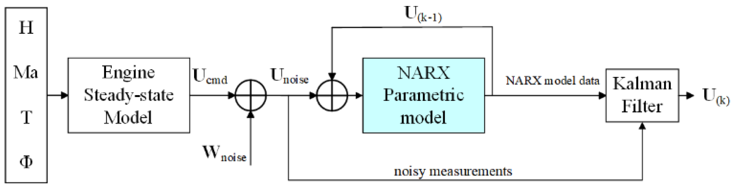
Based on the existing steady state model, the dynamic calibration model based on engine steady state parameters is constructed as shown in Figure 1, where the NARX parameter model is a dynamic artificial neural network, and the parameter register is a stack list for storing the parameter values in the past period of time. The flight test data used for model parameter identification were obtained specifically from dynamic flight conditions during climb and cruise phases, covering altitude ranges of 0–12 km, Mach numbers between 0.3 and 0.85, static temperature differences from −30 °C to 20 °C, and including rapid throttle lever acceleration and deceleration maneuvers.

The model leverages the steady-state model to retrieve both current and historical parameter values from the registers, calculates the predicted values for the next time step, and simultaneously updates the register by storing these values in a stack. This recursive process forms the basis of a dynamic calibration model capable of parallel processing.

The steady-state model derives the steady-state value of the low-pressure rotor speed N1 from the inputs of barometric altitude H, flight Mach number Ma, total atmospheric temperature T, and engine throttle lever angle Φ. U_cmd is the set of the throttle lever angle Φ_cmd and the corresponding rotational speed N1cmd under the steady-state condition, i.e., U_cmd = {Φ_cmd,N1_cmd}. U_old = {Φ_old,N1_old} is the value of the parameter register. U_old = {Φ_cmd,N1_cmd} is the set of parameter values of the past moments stored in the parameter registers of the throttle lever angle Φ and the low-pressure rotor speed N1, where Φ_old = Φ(k), N1_old = [N1(k)...N1(k − u_N1)]T. eold = {Φ_old*,N1_old*} is the set of the dynamically calibrated difference of each parameter’s steady state value in U_old after subtracting the corresponding value, where Φ_old* = Φ_cmd − Φ(k), N1_old* = [N1_cmd − N1(k),...,N1_cmd − N1(k − u_N1)]T. Substituting e_old into the NARX model calculates the predicted difference at the next moment e(k + 1) = {N1*(k + 1)}. Finally, the actual predicted value U(k + 1) = {N1_cmd N1*(k + 1)} = {N1(k + 1)} can be found by subtracting e(k + 1) from the steady state value of N1 in U_cmd.

In actual flight tests, the output U(k + 1) contains a significant amount of measurement noise. To address this, a Kalman filter is introduced to reduce noise in the differential steady-state model. When combined with the Kalman filter, the NARX model becomes more effective at accurately capturing the true state of the dynamic system. This enhancement improves the model’s prediction accuracy and brings it closer to real-world observations. This step is both necessary and effective when dealing with environmental data characterized by high uncertainty and noise.

2.2. NARX Neural Network

The Nonlinear Auto Regressive model with Exogenous Inputs (NARX) neural network is characterized by the presence of Time Delay Layers (TDLs) within each layer of the network, which can be dynamically adjusted to reduce training complexity. This architecture represents a dynamic neural network model that integrates the ARX framework with a multi-layer perceptron (MLP). By leveraging the strong nonlinear mapping capabilities of MLPs and combining them with autoregressive time series input, the NARX model exhibits excellent dynamic behavior. As a result, it is particularly well suited for forecasting complex, nonlinear time series.

The network can be represented by nonlinear difference equations with external inputs:

$$y\left(t\right)=f\left[y\left(t-1\right),\dots ,y\left(t-n_y\right),u\left(t-1\right),\dots ,u\left(t-n_u\right)\right]$$

(1)

where f (·) denotes a specific nonlinear function, y(t − n_y) denotes the corresponding engine model output parameter and the corresponding value of delay n_y, and u(t − n_u) expresses the corresponding engine model input parameter and the corresponding value of delay n_u. As shown in Figure 2, it is mainly composed of input, hidden and output layers and input and output delay layers. The transfer function of the hidden layer is a Sigmoid function and the output layer is a linear function.

$$d_i\left(k\right)=f_{sig}\left(\sum _{r=1}^{n_u}{w}_{ir}\left(k\right)u\left(k-r\right)+\sum _{l=1}^{n_y}{w}_{il}\left(k\right)y\left(k-l\right)+b_i\right)$$

(2)

where f_sig (·) is the hyperbolic tangent Sigmoid function used by the hidden layer nodes; n_u is the prolongation at the external input; n_y is the prolongation at the feedback of the output; w_ir(k) is the weight between the ith hidden layer node and the input u(t − r) at moment k; w_il(k) is the weight between the ith hidden layer node and the output feedback y(t − l) at moment k; and b_i is the ith hidden layer node threshold. The output y_j(k) of the jth output layer node is:

$$y_j\left(k\right)=\sum _{i=1}^N{w}_{ji}\left(k\right)di+T_j$$

(3)

where w_ji(k) is the ith hidden layer node to the jth output layer node weight at moment k; T_j is the jth output layer node threshold; N is the number of hidden layer nodes. The combination of Equations (2) and (3) forms the NARX network expression.

2.3. Steady State Modeling of Engines

As shown in Figure 3, a steady state model of the engine is designed in the Simulink modeling environment; it can be seen that the steady-state engine model contains nine input variables (air pressure altitude ALT_ft, temperature difference dT_C, Mach number, weight-on-wheel signal (WOW), throttle resolver angle (TRA), Approach_Indication, engine lead gas configuration signal, nacelle anti-ice switch NAI, wing anti-ice WAI) and five output variables (thrust, low-pressure turbine speed N1, high-pressure turbine speed N2, fuel flow as FuelFlow, turbine outlet exhaust gas temperature (EGT).

The temperature difference dT_C t refers to the static temperature difference, which is the difference between the static temperature of the aircraft and the temperature of the International Standard Atmosphere (ISA) corresponding to the altitude of the air pressure [33]. This relative temperature is a parameter used to measure the true temperature of the environment in which the aircraft is located using ISA static temperature.

The static temperature difference, pressure altitude, and Mach number are parameters that record the operating environment and conditions of the engine [34,35], so they are selected as input parameters.

The input variables were grounded in first-principles thermodynamics, while correlation analysis was used to complement this foundation by prioritizing TRA over secondary control inputs (e.g., bleed valve position) to maintain model parsimony, and verifying that the correlations between TRA and rotor speed align with theoretical expectations, despite the presence of data noise. This dual approach ensures that the model maintains a balance between physical rigor and fidelity to empirical data.

2.4. Data Filter Smoothing

The moving average filter is employed as a pre-processing step to reduce high-frequency noise in the raw measurements. Although the Kalman filter is effective in handling system and measurement noise within dynamic systems, it is primarily designed for optimal state estimation rather than initial signal smoothing. The moving average filter helps to smooth out rapid fluctuations in the data, thereby improving the initial quality of the inputs to the Kalman filter and enhancing its performance in estimating engine parameters.

The sliding average algorithm (Moving Average) averages a total of 2n + 1 observations before and after the moment to obtain the filtering result at the current moment, which is an intuitive and plain smoothing method, but widely used in practical engineering. For time observation sequence, assuming that each observation is with noise, and the mean of the expected noise is 0 and the variance is σ2, the relationship between the observed value and the true value is as follows:

$$g_t=x_t+{\epsilon }_t$$

(4)

where g_t is the observed value, x_t is the true value, and ε_t is the noise. In order to reduce the effect of noise, the observations of neighboring moments are summed and averaged with the following formula:

$$p_t={\displaystyle \frac{\sum _{i=1}^n\left(x_{t-i}+x_{t+i}\right)+x_t}{2n+1}}$$

(5)

where p_t denotes the filtering result at moment t, $x_{t-1}$ denotes the observed value at moment t − 1 and n represents the sliding window radius. Substituting Equation (4) into (5) yields:

$$p_t={\displaystyle \frac{\sum _{i=1}^n\left(g_{t-i}+g_{t+i}\right)+g_t-\sum _{i=1}^n\left({\epsilon }_{t-i}+{\epsilon }_{t+i}\right)-{\epsilon }_t}{2n+1}}$$

(6)

By assuming that the noise has a mean value of 0, $\sum _{i=1}^n\left({\epsilon }_{t-i}+{\epsilon }_{t+i}\right)+{\epsilon }_t=0$. Therefore, the obtained result is:

$$p_t={\displaystyle \frac{\sum _{i=1}^n\left(g_{t-i}+g_{t+i}\right)+g_t}{2n+1}}$$

(7)

It can be approximated when the change in the true value of the observed data is small:

$$p_t={\displaystyle \frac{\sum _{i=1}^n\left(g_{t-i}+g_{t+i}\right)+g_t}{2n+1}}=g_t$$

(8)

From the above analysis, it can be observed that when the real values within the sliding window remain relatively constant, the filtering method effectively suppresses much of the noise, and the results closely approximate the true values. However, when the real values within the window vary significantly, the filter loses some accuracy, and the output tends to approximate the average trend of the true values. Consequently, the size of the sliding window has a substantial impact on the filtering outcome. A larger window produces a smoother result but introduces a greater deviation from the actual values, while a smaller window retains closer alignment with the observed data but allows more noise to pass through.

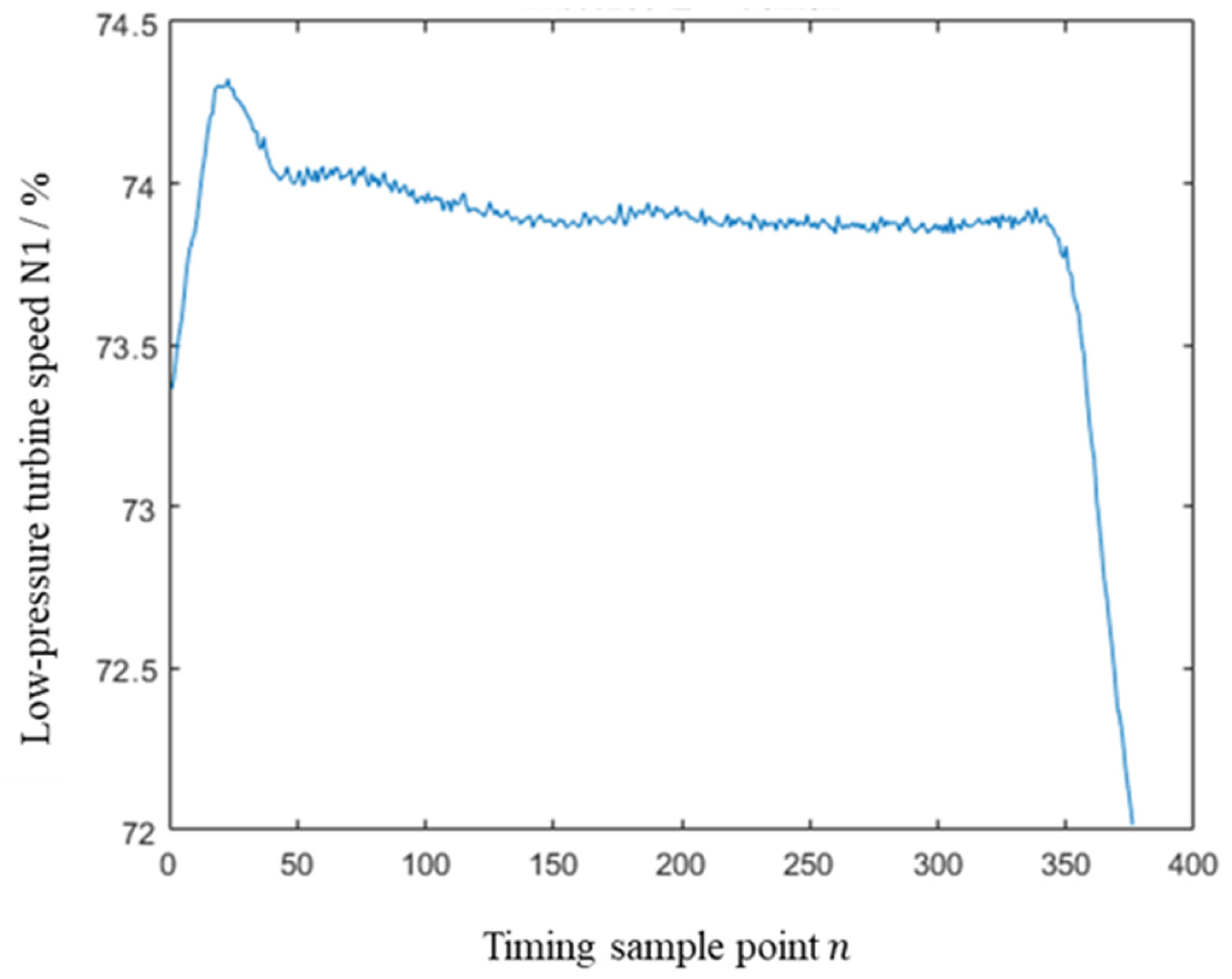
As illustrated in Figure 4, which shows a measurement segment of low-pressure turbine speed (N1), the test signal clearly exhibits the effects of noise.

The existing data are filtered and smoothed by the sliding average algorithm with varying window sizes (3, 11, 21) and the data processing results are observed and evaluated. The original dataset has undergone outlier detection (e.g., 3-sigma criterion and Grubbs’ test) to identify and eliminate gross errors in the experimental data, rather than solely relying on moving average smoothing. This preprocessing step ensures data integrity while preserving the inherent dynamic characteristics of the system. Figure 5 compares results comprehensively for a vast set of data and considers the importance of engine power’s dynamically changing characteristic requirements. The figure also depicts using the sliding average algorithm for smoothening the filtering process and effects of selection of window size of 11. We conducted preliminary experiments to determine an appropriate window width for the moving average filter. These tests were designed to empirically evaluate the trade-off between noise reduction and the preservation of underlying trends in the engine parameter measurements. To investigate the impact of different window widths on signal processing quality, we tested three window widths (3, 11, and 21) for the moving average filter. The evaluation was based on the root mean square (RMS) error and the frequency response characteristics of the filter. After comprehensive analysis, a window width of 11 was selected, as it demonstrated the optimal performance, effectively balancing noise reduction with the preservation of critical signal features. Based on the experimental results and practical considerations, a window width of 11 observations was selected, as it effectively balanced noise suppression with the timely detection of true parameter variations. Therefore, this window length is best for smoothing filtering effect, to minimize the impact of noise on a measured value, and can also maintain dynamic realism.

2.5. Data Classification and Aggregation

The push rod has two states: “push” and “pull”. Since the dynamic changes under the corresponding states are not identical, they need to be extracted separately for the identification of either type of dynamic system.

In order to better extract the features of datasets, the correlation between the throttle resolver angle TRA, temperature difference T, altitude h, flight Mach number Ma, the engine speed and power change is first investigated, in an attempt to determine the most representative variable for feature extraction and classification. The Pearson correlation coefficient is used for correlating between the above measured variables and the engine low-pressure turbine speed. It is used to measure the correlation between two variables and is calculated by simple linear regression estimation. The value of Pearson’s correlation coefficient ρ varies within the range of [−1, 1]; when the value is positive, the two observed variables are positively correlated, and when the value is negative, the two variables are negatively correlated. The larger the absolute value, the higher the correlation between the two variables, and an absolute value of the coefficient at [0.8, 1] is usually considered to represent a strong correlation.

Firstly, the Pearson’s correlation coefficient between the throttle lever angle TRA, temperature difference T, altitude h, flight Mach number Ma and low-pressure turbine speed N1 is calculated by using the provided test flight data, importing each set of test flight data in MATLAB_R2021b and using the corr-function to carry out the calculations. The algorithm requires that the dimensionality of the two variables be equal, and the results of the calculations are shown in

Table 1. Pearson’s correlation coefficients of variables with N1.

	$\mathit{T}\mathit{R}\mathit{A}$	$\mathit{T}$	$\mathit{h}$	$\mathit{M}\mathit{a}$
$\rho$	0.84	0.67	−0.69	0.71

.

The correlation coefficients between the TRA, temperature difference T, altitude h, flight Mach number Ma and the high-pressure turbine speed N2 were then calculated using the data provided for the test flight, and the results are shown in

Table 2. Pearson’s correlation coefficients of variables with N2.

	$\mathit{T}\mathit{R}\mathit{A}$	$\mathit{T}$	$\mathit{h}$	$\mathit{M}\mathit{a}$
$\rho$	0.97	0.62	−0.66	0.70

.

Observing the above two tables, it can be seen that the TRA is the most correlated and strongly correlated with the engine output power (low-pressure turbine speed N1 and high-pressure turbine speed N2) among all the observed measurement variables. Therefore, the throttle lever angle TRA is selected as the examined variable for dynamic feature extraction and classification.

By observing the trend of feature segment data, a dynamic state identification extraction method (Trend Intercept Method) is proposed. The extraction algorithm, under the precondition of confirming the test flight data weight-on-wheel signal WOW = 0 (in the empty state), initially filters out the sampling point sequences of the trend segments in line with the trend segments of “fast push lever” and “fast pull lever” according to the amount of the change of the throttle lever angle in the length of a fixed period of time. It then determines the sampling point of the starting change of the throttle lever in each set of trend data as the starting point of change n0. Under the premise of “fast push lever” and “fast pull lever”, the sequence of sampling points is initially filtered by the amount of change in the length of the throttle lever angle in a fixed period of time to determine the sampling point that corresponds to the trend segment of “fast push lever” and “fast pull lever”, and then the sampling point of the starting point of the throttle lever change is identified as the starting point of the change in the trend data in each trend data segment. This method avoids inefficient differential traversal of a large volume of test flight data, saves computational and time resources in the form of magnitude, and greatly improves the extraction efficiency, while having better physical interpretability.

Figure 6 shows the intercepted first section of the rising edge of the push rod and Figure 7 shows the intercepted first section of the falling edge of the tie rod. They have a good physical interpretation of the significance and the length of the interception is different, and can completely intercept the high-pressure and low-pressure turbine speed changes in the reaction data dynamic response. In Figure 7, it is shown that during deceleration, the speed of the low-pressure rotor does not remain constant, but its variation amplitude is not large enough relative to the high-pressure rotor. From the image, it can be seen that the low-pressure rotor shows a decreasing trend in speed, just like the high-pressure rotor, at 0–80 sampling time points. In the post-80s segment of Figure 7, the low-pressure rotor (N1) increases despite TRA reduction due to the following factors. Fuel control logic: During deceleration, the engine control unit prioritizes high-pressure rotor (N2) stability to prevent surge. This temporarily increases N1 via bleed valve adjustments. Altitude compensation: As the aircraft descends, rising ambient pressure reduces N2’s load, allowing N1 to recover. The NARX model captures this coupling through delayed feedback of N2 and Mach number inputs. On this basis, different data labels are given to the rising edge and the falling edge, respectively; the rising edge label is recorded as 0 and the falling edge label is recorded as 1 to complete the data classification.

2.6. Kalman Filter

The Kalman filter is an efficient optimality estimator (a set of mathematical equations) that provides a recursive computational method for estimating the state of a discrete data control process, usually from noisy measurements, and offers uncertainty of an estimate. We opted for a recursive algorithm (Kalman filter) over a one-step method (such as regularized least squares) primarily based on the following considerations. The Kalman filter is well suited for online applications, as it can incrementally process new data, whereas regularized least squares typically requires all data to be input at once. This is because, for large-scale data, the recursive algorithm processes only one data point at a time, resulting in lower computational load, while regularized least squares requires processing the entire dataset, leading to higher computational complexity. The Kalman filter is usually suitable for the following circumstances: (1) measuring a variable that cannot be measured directly; (2) measuring a variable that is usually obtained from several noisy indirect variables. The Kalman filter is divided into two steps:

Time update equations:

$${\widehat{\mathit{x}}}_{k+1}^{-}={\mathit{A}}_k{\widehat{\mathit{x}}}_k+\mathit{B}{\mathit{u}}_k$$

(9)

$${\mathit{P}}_{k+1}^{-}={\mathit{A}}_k{\mathit{P}}_k{\mathit{A}}_k^T+{\mathit{Q}}_k$$

(10)

Measurement update equations:

$${\mathit{K}}_k={\mathit{P}}_k^{-}{\mathit{H}}_k^T{\left({\mathit{H}}_k{\mathit{P}}_k^{-}{\mathit{H}}_k^T+{\mathit{R}}_k\right)}^{-1}$$

(11)

$${\widehat{\mathbf{x}}}_k={\widehat{\mathit{x}}}_k^{-}+\mathit{K}\left({\mathit{y}}_k-{\mathit{H}}_k{\widehat{\mathit{x}}}_k^{-}\right)$$

(12)

$${\mathit{P}}_k=\left(\mathit{I}-{\mathit{K}}_k{\mathit{H}}_k\right){\mathit{P}}_k^{-}$$

(13)

where “^-” and “ˆ” denote a priori estimation and a posteriori estimation, respectively, P is the estimated error covariance of the estimated state vector, and the posterior estimate error covariance quantitatively reflects the quality of the state prediction. $\mathit{K}\in {\mathbb{R}}^{n\times m}$ is the Kalman gain, which provides the weight correction between the measurement and the prediction by minimizing the trace of posterior error covariance P_k. I is the identity matrix. The term ${\mathit{y}}_k-{\mathit{H}}_k{\widehat{\mathit{x}}}_k^{-}$ refers to innovation or residual, and describes the difference between predicted measurement and actual measurement.

In aircraft flight, the sensor data are often difficult to collect accurately due to the harsh environment. The direct input of highly fluctuating sensor signals into the NARX model for modelling may lead to insufficient model accuracy. Therefore, it is reasonable to apply Kalman filter to data fusion of the NARX model output and the noise-bearing input signals to achieve noise reduction.

3. Results

3.1. Dataset Organization

Using NARX neural network, experimental test flight data were preprocessed for data cleaning, fusion, classification and pooling. Later on, the “fast push-pull” engine data were generated according to the targeted boundary conditions (intercepting and recording the throttle TRA, temperature difference δt, and altitude h). Moreover, four inputs (Mach number Ma, low-pressure turbine speed N1, high-pressure turbine speed N2, low-pressure turbine outlet exhaust gas temperature EGT) and five physical quantities (weight-on-wheel signal WOW, Approach Indication, Engine Cavitation Configuration (ECS), Wing Anti-Ice WAI, and Nacelle Anti-Ice Switch NAI) were also recorded. Since the test flight data generation process simultaneously records data for left and right engines and also the operation of throttles of these engines is not completely synchronized, the data of the left and right engines under the same acquisition process are considered as two sets of data for the sake of this study. In order to test the ability of NARX neural network to solve the complex time-dependent system prediction problem with multivariable and highly nonlinear dynamics of aircraft engines, firstly, we take the test flight data as samples, and try to use the throttle TRA, the temperature difference δt, the altitude h, and the flight Mach number Ma as the inputs, and then run the simulation and observe the effects of the low-pressure turbine rotation speed N1 and the high-pressure turbine rotation speed N2.

For instance, consider the rising edge of “fast pusher” for analysis. A total of 10 fast-acceleration datasets were captured from the categorized experimental data. In these ten datasets, each set includes multiple throttle adjustment segments transitioning from low thrust to high thrust, as well as throttle adjustments during different flight phases (such as climb, cruise, and approach), totaling 152 segments. Consequently, each set provides numerous representative training samples. The diversity of scenarios enables the model to fully capture the nonlinear coupling between external meteorological conditions (e.g., temperature, altitude, and Mach number) and engine characteristics. 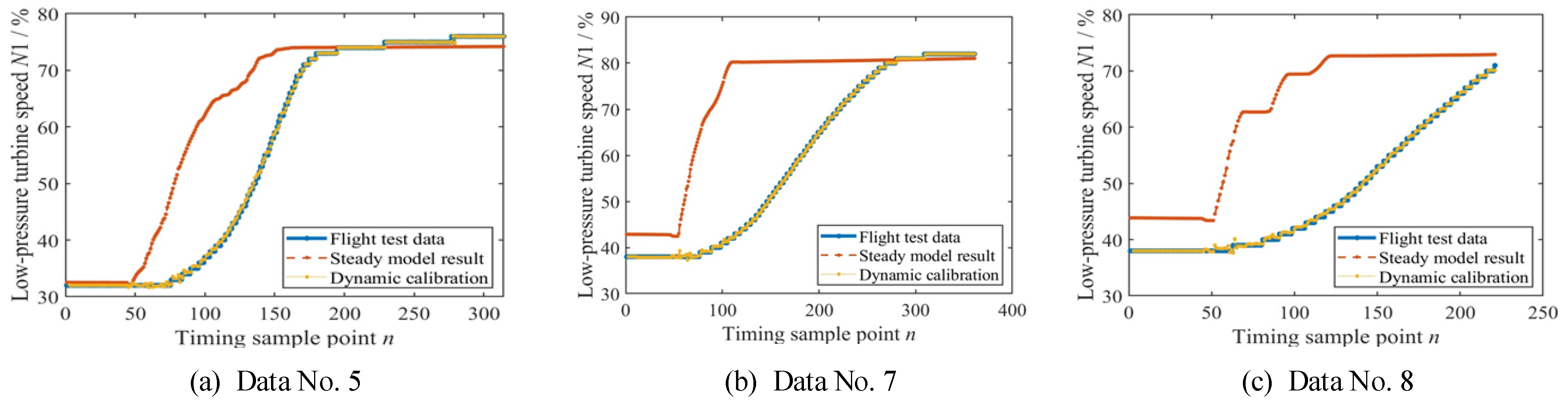Figure 8 shows the effects of changing the throttle lever position on each acceleration segment. Similarly, Figure 9 presents the effects of low-pressure turbine and high-pressure turbine speeds on the captured segments. These trending graphs show that the duration of each group of data is different from the other and hence suggest different data lengths. It was observed that variations of datasets of 5, 7 and 8 are within the overall operating conditions of the envelope graph and therefore were selected for testing purposes, while the remaining datasets were reserved for training to test the effectiveness of the NARX neural network.

After synthesizing the comparison of the single-data single-input training network effect, single-data multiple-input training network effect, and multiple-data single-input training network effect, the neural network effect with multiple data and multiple inputs is obtained. Experiments were conducted with TRA, air pressure altitude h, temperature difference δt, Mach number Mach as inputs and low-pressure turbine speed N1 as output. The training and test datasets were also divided in a ratio of 7:3. After observing that the variation ranges of datasets 5, 7 and 8 are inside the overall wrap-around plot, these were selected for testing, and the rest of the seven datasets were used for training. Through iterations, the model obtained from training is considered to meet the simulation criteria when the resultant (mean square error, MSE) value is below 5.

3.2. Engine Dynamic Calibration Modeling

The above “fast pushrod” acceleration data are input into the steady-state calibration model, and the output and the experimental data of the test flight are calculated and further input into the NARX network in an attempt to test the effect of multiple datasets and multiple inputs to train the network. To further test the robustness and generalization effect of the model, the flight parameter dataset was randomly divided into 10 training and testing sets, and all data in the testing set were modeled and validated. The maximum relative errors of output parameters N, Nz and EGT, the average relative errors of Ti and Tt, and the maximum RMSE of 10 test results were obtained. By using this type of cross-validation, the evaluated model can be made more accurate and reliable. Moreover, experiments are carried out with the low-pressure turbine’s rotor speed deviation steady-state difference ΔN1, the high-pressure turbine’s rotor speed deviation steady-state difference ΔN2, and low-pressure turbine outlet exhaust temperature deviation ΔEGT as inputs and low-pressure turbine’s rotational speed difference ΔN1 as output. The Exit Exhaust Temperature Bias Steady State Difference ΔEGT and Low-Pressure Turbine Speed Difference ΔN1 were also used as input and output, respectively, for the experiment. The training and test datasets are also divided in a ratio of 7:3. After observing that variation ranges of datasets 5, 7 and 8 are inside the overall envelope plot, these are selected for testing, and the remaining seven datasets are used for training. The biased steady state output results are then used to calculate the difference with the steady state model to complete the dynamic calibration model pathway construction and realize the steady-state difference correction function.

As shown in Figure 10, taking the performance of the low-pressure turbine speed N1 for example, the dynamic calibration model output is compared with the actual test flight data. Observing the graph, it can be seen initially that the error between the output of the dynamic calibration model and the actual flight output is relatively small, and the specific model’s performance needs to be further calculated using a determination algorithm. The dynamic calibration model is based on engine steady-state parameters, and the difference between the output of the steady-state model and the actual test flight data is used as the training input of the NARX neural network. By comparing the outputs of the NARX neural network and the steady-state model, the dynamic calibration parameters of the engine (such as low-pressure turbine speed N1, high-pressure turbine speed N2, etc.) can be obtained to complete the overall development of the dynamic calibration model for engine parameters.

According to the reference standard [36], as shown in Figure 11 of the article, the dynamic characteristics of the engine model obtained by introducing dynamic characteristic index parameters Ti and Tt were validated and verified for their superiority and inferiority. Record the complete process of dynamic changes in the engine output parameter Y, with the origin of the horizontal axis being the starting time of the throttle lever change, where t1 is the time when parameter Y reaches 10% of its response, t2 reaches 90% of its response, Ti is the time period from 0 to t1, and Tt is the time period from t1 to t2. Calculate Ti and Tt separately for real flight data and identification dynamic models. According to the “Performance Standards for Aircraft Flight Simulator Identification” [37], when the relative error between the two is within ± 10%, it is determined that the engine dynamic model meets the simulation testing standards, and the smaller the relative error, the more realistic the dynamic characteristics of the model.

The dynamic characteristics of the engine system model “fast push-pull lever” calibrated by the algorithm should be able to satisfy the following indexes: when examining the acceleration characteristics of the push-pull lever, it should record the engine power during the period of thrust from the jogging vehicle to the restart of the flight (N1, N2, etc.). As a result, it moves the throttle lever quickly during the operation, records Ti (as from the beginning of moving the throttle to the key engine parameters to achieve its response to 10% of the total time, Tt, where Tt is the total time from Ti to 90% of the power of the restart), and requires the corresponding model outputs (Ti_model and Tt_model) and the experimental flight data to differ within ±10% or 0.25 s. The schematic diagram of Ti versus Tt is shown in Figure 11. Similarly, when examining the characteristics of tie rod deceleration, the engine power is recorded from the maximum takeoff power to 10–90% of maximum. As a result, it moves the throttle lever quickly during the operation, records Ti (as from the beginning of moving the throttle to the key engine parameters to achieve its response to 90% of the total time, Tt, where Tt is the total time from Ti to 10% of the power of takeoff), and requires the corresponding model outputs (Ti_model and Tt_model) and the experimental flight data to differ within ±10% or 0.25 s.

The maximum speed of the low-pressure turbine in this acceleration section is N1t, and the simulation and physical tests are conducted to reach 10% N1t (for corresponding time Ti_model and Ti, respectively). According to the performance requirement benchmark, the requirement is that |Ti_model − Ti| ≤ 10% of (Ti − T0) or |Ti_model − Ti| ≤ 0.25 s. Similarly, the simulation and physical tests are conducted to reach 90% N1t (for corresponding time Tt_model and Tt, respectively). 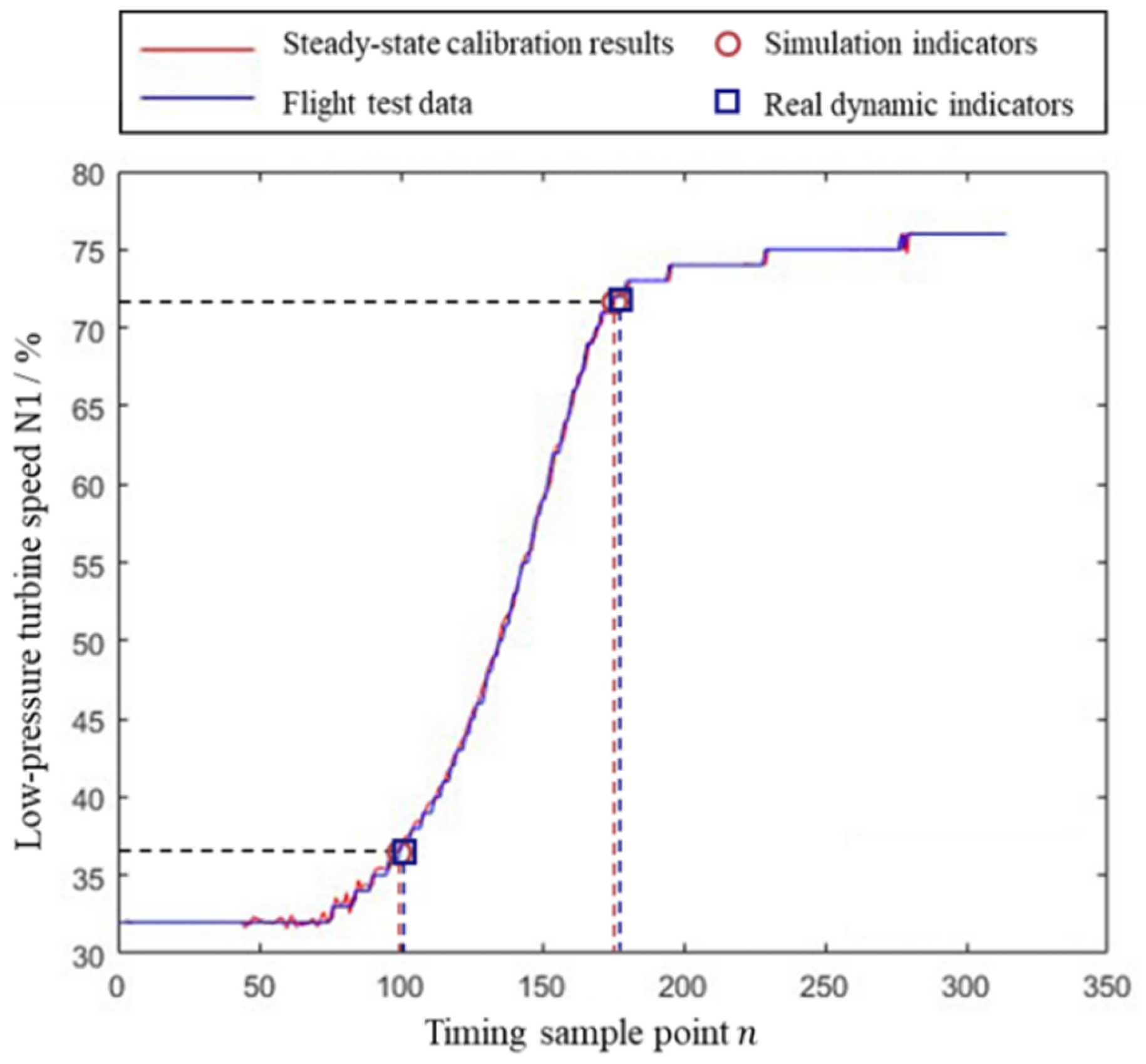According to the performance requirement benchmark, the requirement here again is |Tt_model − Tt| ≤ 10% of (Tt − T0) or |Tt_model − Tt| ≤ 0.25 s. Taking the test data No. 5 as an example, the dynamic characteristic simulation results are shown in Figure 12, in which the real test flight data and the simulation output are shown, respectively. The Ti and Tt values of the real and simulated outputs are calculated according to the criteria described above. The results show that the relative errors of Ti and Tt are less than 5%, respectively, which meets the performance requirements of the aircraft flight simulator. Validation results across multiple test cases confirm that the model satisfies the ±10% Ti/Tt error tolerance under varying TRA rates, demonstrating its robustness within the operational envelope. The simulation results of other test data show a pleasant dynamic response fidelity, which verifies the accuracy of the proposed method in simulating the dynamic change characteristics.

When designing the algorithm, since the record is based on sampling points rather than continuous time points, it is necessary that the judgment be made through an iterative loop to find the sampling point closest to the targeted power (e.g., N1, 10% N1, 90% N1, and other specific size of the power parameter) to be recorded as the corresponding time point. At the same time, it should be noted that when examining whether the 0.25 s performance judgment criterion is being fulfilled, a 32 Hz sampling frequency should be used as the sampling point interval and time length of the conversion.

3.3. Denoising NARX Noisy Data Using Kalman Filter

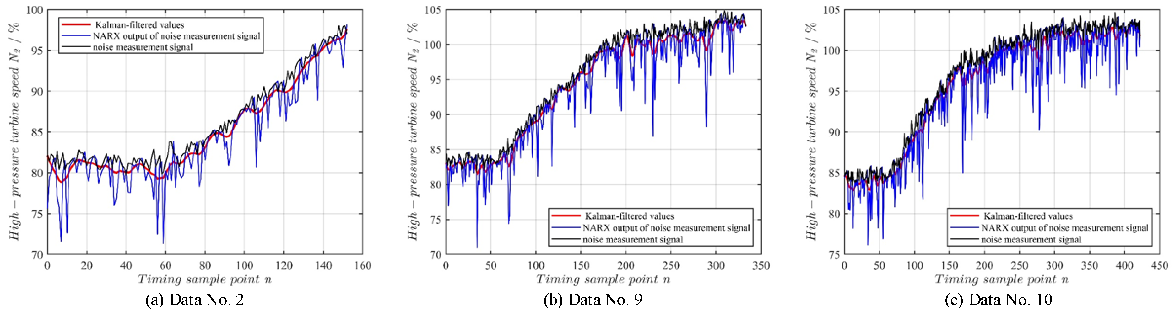
In order to simulate the noise background of the sensor measurement, Gaussian noise is introduced to the smoothed high-pressure turbine speed of the INPUT_N2 signal to simulate the real environment. The signal-to-noise ratio (SNR) is set to below 45 dB to simulate strong background noise conditions. Then, the noise signal is fused with the predicted signal OUTPUT_N2 from the NARX model to obtain a new N2 signal, called Kalman_N2 signal. Datasets No. 2, 9 and 10 are selected for demonstration.

By feeding the noise signal N2 noise and the filtered signal Kalman_N2 into the trained NARX model simultaneously, we obtain the corresponding output values. After comparing these two output values with the original NARX predictions, it is observed that the Kalman filtered NARX values are closer to the actual values. Datasets No. 2, 9 and 10 are selected for demonstration, as shown in Figure 13.

4. Discussion

While the model replicates engine responses to TRA inputs recorded from operator actions in flight tests, it does not explicitly include the operator as part of the system. The dynamic parameters (e.g., time constants) are derived solely from the engine’s physical response to TRA changes under experimental conditions.

The model’s generalization is demonstrated through the following. Cross-validation: 10-fold testing showed consistent MSE <5% across altitude (0–12 km) and Mach (0.3–0.85) ranges. Environmental robustness: The temperature difference term accounts for ISA deviations, enabling adaptation to −30 °C to 20 °C variations. Noise immunity: Kalman filtering ensures stability under SNR < 45 dB.

The results of this experiment show that the NARX model is more capable of reflecting the actual state of the dynamic system when the Kalman filter is used. By effectively removing the effect of noise on the model, the Kalman filter helps to improve the predictive accuracy of the model and bring it closer to the actual observations. This further validates the effectiveness of Kalman filtering in data fusion, especially when dealing with real environmental data of high uncertainty and noise.

5. Conclusions and Future Work

In the current study, a data fusion method is proposed to dynamically predict the rotor speed of an automatic control system. The NARX model is applied to an existing steady model for the correction of dynamic response. In addition, a Kalman filter is applied to fuse the noise measurement data and prediction from the dynamic model. As such, the proposed method can dynamically predict the high-pressure and low-pressure rotor speed N1 from the inputs of barometric altitude h, flight Mach number Ma, total atmospheric temperature T, and engine throttle lever angle Φ, even with strong background noise in the measurement.

(1)

By comparing the flight test record data and the prediction output of the dynamic model, it is found that the combination of NARX and steady automatic control system model can achieve an accuracy below 5% for testing data. The high accuracy implies that the dynamic response model identification method has strong generalization ability and meets the accuracy requirements of practical applications.

(2)

At the same time, the NARX model has good dynamic characteristics, and the maximum relative errors of its dynamic parameter indicators Ti and Tt are less than 5%, respectively, and the output has higher prediction accuracy in time series.

(3)

Gaussian noise is introduced to simulate noise measurement conditions. The results of this experiment show that the NARX model is more capable of reflecting the actual state of the dynamic system when the Kalman filter is used, even with low signal-to-noise ratio SNR < 45 dB.

The model still faces some notable challenges and limitations. First, to achieve an accurate prediction, a relatively short time step is adopted, allowing the NARX model to forecast a smaller time span at each iteration and thus reduce the likelihood of error accumulation. Furthermore, the collected data do not fully encompass extreme or rare operating conditions—such as conducting complex maneuvers at very high altitudes or under extremely low temperature corrections—and the modeling of external parameters and engine performance is based on simplified assumptions that cannot account for all real flight scenarios. In addition, the current research only models engine acceleration and deceleration during climb and cruise, lacking an in-depth investigation of thrust output and engine dynamics during takeoff and landing. Furthermore, the current model does not yet consider factors such as throttle rate of advance.

Given these limitations, future work will focus on predicting for a longer time, collecting larger and more diverse real-world flight test data, further refining the integration of external environmental conditions and operational variables into the modeling process, and introducing new input variables to enhance the model’s performance under different operational profiles. By doing so, we aim to continuously improve the model’s generality, robustness, and engineering applicability.