Transonic Dynamic Stability Derivative Estimation Using Computational Fluid Dynamics: Insights from a Common Research Model

Abstract

Dynamic stability derivatives are critical parameters in the design of trajectories and attitude control systems for flight vehicles, as they directly affect the divergence behavior of vibrations in an aircraft’s open-loop system when subjected to disturbances. This study focuses on the estimation of dynamic stability derivatives using a computational fluid dynamics (CFD)-based force oscillation method. A transient Reynolds-averaged Navier–Stokes solver is utilized to compute the time history of aerodynamic moments for an aircraft model oscillating about its center of gravity. The NASA Common Research Model serves as the reference geometry for this investigation, which explores the impact of pitching, rolling, and yawing oscillations on aerodynamic performance. Periodic oscillatory motions are imposed while using a dynamic mesh technique for CFD analysis. Preliminary steady-state simulations are conducted to validate the computational approach, ensuring the reliability and accuracy of the applied CFD model for transonic flow. The primary goal of this research is to confirm the efficacy of CFD in accurately predicting stability derivative values, underscoring its advantages over traditional wind tunnel experiments at high angles of attack. The study highlights the accuracy of CFD predictions and provides detailed insights into how different oscillations affect aerodynamic performance. This approach showcases the potential for significant cost and time savings in the estimation of dynamic stability derivatives.

1. Introduction

In the field of aircraft design and development, achieving dynamic stability within the flight envelope is both challenging and expensive. For transonic flight, particularly, the interaction between shock wave induced separation, swirling motion, and flow rupture generates complex, unsteady, and nonlinear fluid dynamics. These interactions often result in aerodynamic effects that exceed simple expectations, sometimes leading to unexpected and significant outcomes. During the aircraft design phase, predicting the limits of dynamic operational stability and the intensity of potential dynamic issues is arduous, with many issues only becoming apparent during the flight testing stage. This fact directly results in an extended aircraft design cycle, a substantial increase in design costs, and negative impacts on overall performance.

The significance of these challenges becomes particularly pronounced for fighter aircraft, which demand exceptional maneuverability and operability at a high angle of attack (AoA), as well as for tailless stealth aircraft, which are prone to exhibiting unsteady dynamic behaviors. For traditional aircraft operating at relatively low speeds and small AoA, static stability derivatives are adequate to estimate the moments produced during maneuvers [1]. However, at higher AoA, nonlinear aerodynamic effects such as boundary layer separation, vortex oscillation, and vortex breakdown are inevitable. Moreover, these phenomena are particularly important in transonic or supersonic flow regimes, where the formation of shock waves is more likely to occur [2].

Developing improved flight models requires an aerodynamic framework with precise dynamic derivatives, particularly for high-AoA flight regimes, where these parameters play a crucial role in influencing flight performance [3]. Dynamic derivative information has traditionally been obtained through flight tests, although these are often expensive and carry significant risk [4]. An alternative method that has been extensively utilized involves using wind tunnel experimental data to determine dynamic stability derivatives [5]. However, the wind tunnel testing approach, while valuable, has notable limitations and can become expensive due to the complexity of experimental setups required to replicate various dynamic motions. Furthermore, it is crucial in the experiments to remove the inertial forces generated by the oscillating test model from the aerodynamic data in order to ensure accurate measurements. Achieving this result requires precise synchronization between the motion history and the recorded moment data. Even a minor mismatch in synchronization can introduce significant errors in dynamic derivative calculations, necessitating an exceptionally accurate and meticulously designed experimental setup. Additionally, scaling challenges and support interference issues present further complications in wind tunnel testing. These challenges are particularly pronounced at high AoAs and for high Mach number conditions, where they impede accurate predictions of the model’s aerodynamic characteristics. Another critical limitation arises from delays in measurement data due to the mechanical nature of the vibration devices, which can introduce errors. These factors collectively highlight some of the primary constraints associated with wind tunnel testing [6,7].

On the other side, recent advancements in computational power and technology have made it possible to analyze dynamic stability derivatives using applied computational fluid dynamics (CFD) methods, addressing the above-mentioned limitations. Specifically, progress in computational capacity, along with innovations in moving grid techniques, like dynamic meshing, enables the high-dimensional study of more intricate flight vehicle models. Practically, these advancements strengthen the efficiency and accuracy of numerical analysis for evaluating dynamic stability derivatives [7,8]. A significant portion of recent research in this field focuses on developing efficient approaches to calculate combined dynamic stability derivatives, especially concerning pitch damping coefficients.

The concept of stability in aerodynamic derivatives within the linear range of small disturbances was initially proposed by Bryan [9], who suggested that aerodynamics and flight dynamics can be considered separately, allowing the aerodynamic forces and moments to be expressed as functions of various static and dynamic factors, such as disturbance velocities, control angles, and their rates of change. Early analytical approaches were applied to simple two-dimensional configurations, such as Theodorsen’s method for analyzing wing sections [10]. This approach has since been refined to better identify directional and sideslip derivatives, for instance, for flow around a thin airfoil at supersonic speed [11].

Additionally, time domain techniques can be utilized to assess dynamic stability derivatives by solving the unsteady flow field and its associated time-dependent parameters, often utilizing a forced oscillation method [12]. The method involves inducing oscillations in an aircraft model around its center of gravity, maintaining a constant angular displacement magnitude. In this context, one of the straightforward displacement techniques available is the simple harmonic oscillation (SHO) method. This approach involves inducing oscillations with simple harmonic motion. By doing so, the unsteady aerodynamic forces, computed using CFD tools, can be applied to determine the dynamic stability derivatives [13]. However, these computations are particularly challenging due to the complexity of the unsteady flow field to be reproduced. Traditional calculation methods typically include fast engineering calculations [14], linear frequency domain methods [15], nonlinear frequency domain methods [16], and high-precision time domain predictions [6]. While these methods provide simplified approximations of time domain CFD calculations, they are not well suited for capturing the nonlinear behavior of complex configurations. Indeed, accurate unsteady simulations require accounting for the significant role of viscosity effects within the internal flow field. Complex flows arise from shock wave–boundary layer interactions, and flow nonlinearity is highly apparent. Given the limited prior knowledge on the dynamic simulation of internal flows, time domain accurate prediction, representing the most advanced level of nonlinear aerodynamic behavior prediction, emerges as the optimal choice for dynamic unsteady calculations.

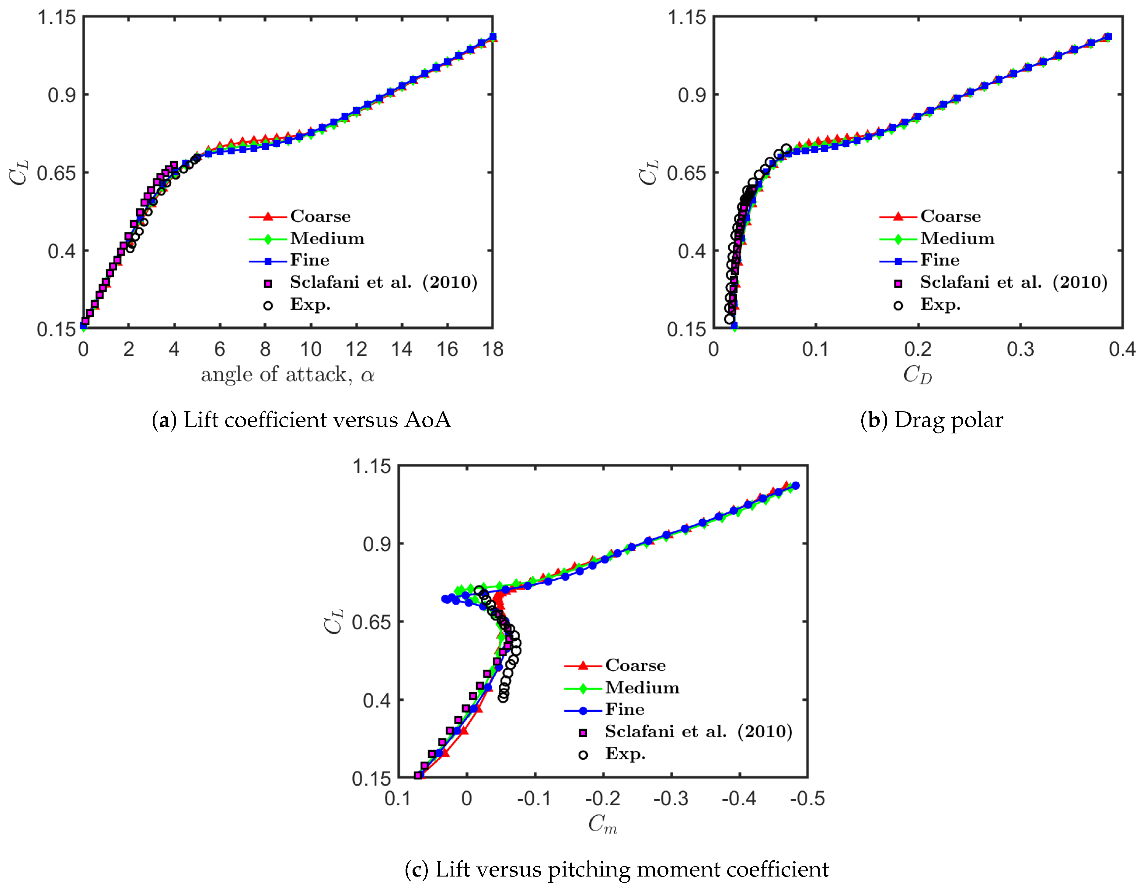
In this complex scenario, the Reynolds-averaged Navier–Stokes (RANS) equations can be employed to simulate the unsteady flow field for vehicle simple harmonic vibrations, studying the aerodynamic behavior under oscillatory motions. The unsteady RANS approach, supplied with the proper closure turbulence model, has been often utilized for dynamic stability analysis in aerospace industry, e.g., [17,18,19]. Here, the forced SHO approach is applied for the transonic flow regime, with the NASA Common Research Model (CRM) serving as the base geometry. Three different oscillation modes (pitching, rolling, and yawing) are designed to isolate specific dynamic stability derivatives by applying harmonic motion around the corresponding principal axis. The CFD setup employs a dynamic meshing technique, with user-defined functions (UDFs) controlling the harmonic motion inputs to simulate the oscillatory behavior of the aircraft model.

The objective of this study is to demonstrate the effectiveness of the forced SHO method in calculating dynamic stability derivatives under complex flow conditions. This approach is significant compared to traditional methodologies because it allows for more accurate capturing of the nonlinear behavior of the aerodynamic flow field, particularly in the transonic regime, where shock waves and boundary layer interactions are prevalent. Additionally, using CFD for dynamic stability derivative estimation offers a cost-effective and safer alternative to wind tunnel and flight tests, which are often expensive and risky. This method also enables precise synchronization between motion history and recorded moment data, reducing errors in dynamic derivative calculations, and enhancing the reliability of the results. The present research focuses on the estimation of dynamic stability parameters using transient CFD within the transonic regime and at high AoAs. The current analysis aims to provide valuable insights into the longitudinal and lateral-directional responses of the aircraft model, contributing to a deeper understanding of its dynamic behavior under complex flow conditions.

The remainder of this paper is organized as follows. Section 2 provides an overview of the methodology employed, detailing the implementation of forced harmonic oscillations and the computational framework used to extract dynamic stability derivatives. In Section 3, the complete applied CFD model is presented, including the description of the simplified geometry, the mesh generation process, and the simulation setup. Section 4 discusses the results and analysis, covering the validation of the CFD model, the evaluation of aerodynamics characteristics, and the analysis of dynamic stability derivatives for different oscillatory motions. Section 5 offers some concluding remarks.

2. Methodology

This study employs the forced SHO method to investigate unsteady aerodynamic characteristics through controlled periodic motions. Specifically, three types of simple harmonic oscillation are considered: rolling, pitching, and yawing. The rotation axes are corresponding to the three principal axes of rotation, namely, the longitudinal X axis, lateral Y axis, and vertical Z axis. By conducting simulations of these basic oscillations, the corresponding unsteady aerodynamic responses can be systematically analyzed, allowing for the independent extraction of dynamic stability derivatives for each primal axis. These parameters play a crucial role in characterizing the stability and control behavior of the aircraft, as the dynamics of flight vehicles depend on the structure’s reaction to the time-varying aerodynamic forces and moments. Importantly, current oscillations at controllable frequencies provide a systematic and reproducible approach for analyzing aerodynamic responses. 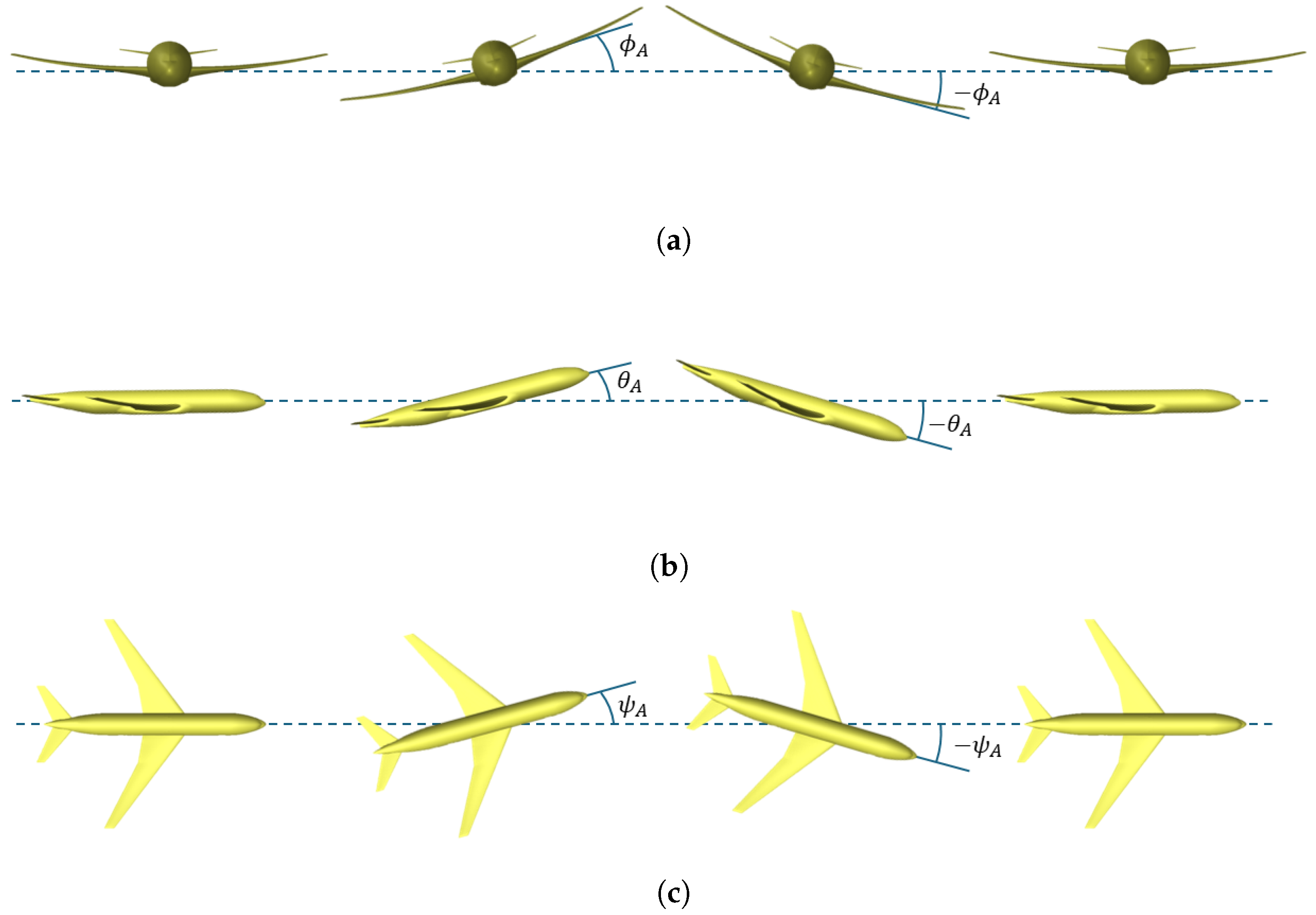Figure 1 visually represents the three different modes of simple harmonic motions employed, with $\varphi$, $\theta$, and $\psi$ representing the associated varying angular positions, namely, the pitch, roll, and yaw angles.

2.1. CFD Implementation

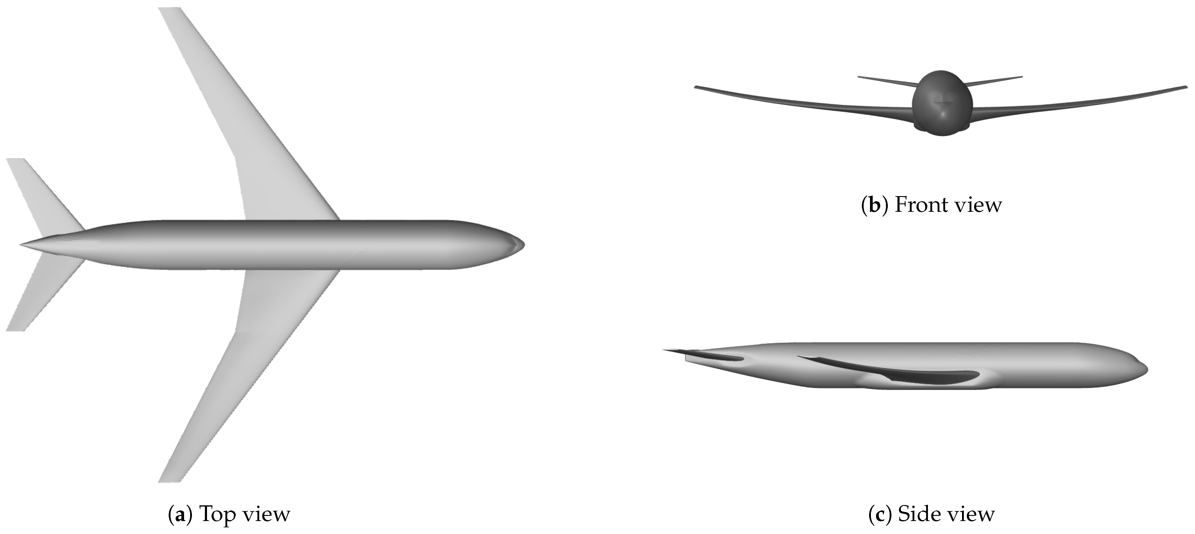
The three different harmonic motions are implemented into the applied CFD model through UDF procedures written in C programming language. These ad hoc functions are tailored to the different oscillation modes associated with the reference system depicted in Figure 2. Each UDF procedure precisely controls the corresponding oscillation parameters (amplitude, frequency, and phase), ensuring the accurate representation of the prescribed motion of the aircraft model. Basically, each UDF defines the angular velocity for each simple mode, without imposing any translational motion, thus allowing for the pure rotation around the longitudinal, lateral, or vertical axis, as required for the stability analysis. This procedure ensures that the motion remains purely angular and does not interfere with translational velocity components in the system. The three different oscillations are shown in

Table 1. Oscillations imposed by the three different user-defined functions.

Mode	Rolling	Pitching	Yawing
X-axis rotation	$\varphi \left(t\right)={\varphi }_{A}sin\left(\omega t\right)$	-	-
Y-axis rotation	-	$\theta \left(t\right)={\theta }_{A}sin\left(\omega t\right)$	-
Z-axis rotation	-	-	$\psi \left(t\right)={\psi }_{A}sin\left(\omega t\right)$

, where ${\varphi }_A$, ${\theta }_A$, and ${\psi }_A$ represent the rolling, pitching, and yawing amplitudes, respectively, while $\omega$ stands for the constant angular velocity. Specifically, the pitching motion captures longitudinal stability characteristics, the rolling motion addresses lateral stability, and the yawing motion evaluates directional stability.

To accommodate the above oscillatory motions in the current numerical simulations, a moving dynamic mesh approach is employed. The dynamic mesh is updated at each time step, using smoothing and remeshing algorithms, to maintain mesh quality and prevent element distortion during oscillations. The use of a dynamically adjusted mesh for the ongoing simulations is crucial to maintain the quality of the computations, as the deformation of the geometry during the motion must be accurately reflected by the numerical grid. This approach ensures a comprehensive assessment of the unsteady aerodynamic response for the three primary axes of motion.

2.2. Evaluation of Dynamic Stability Derivatives

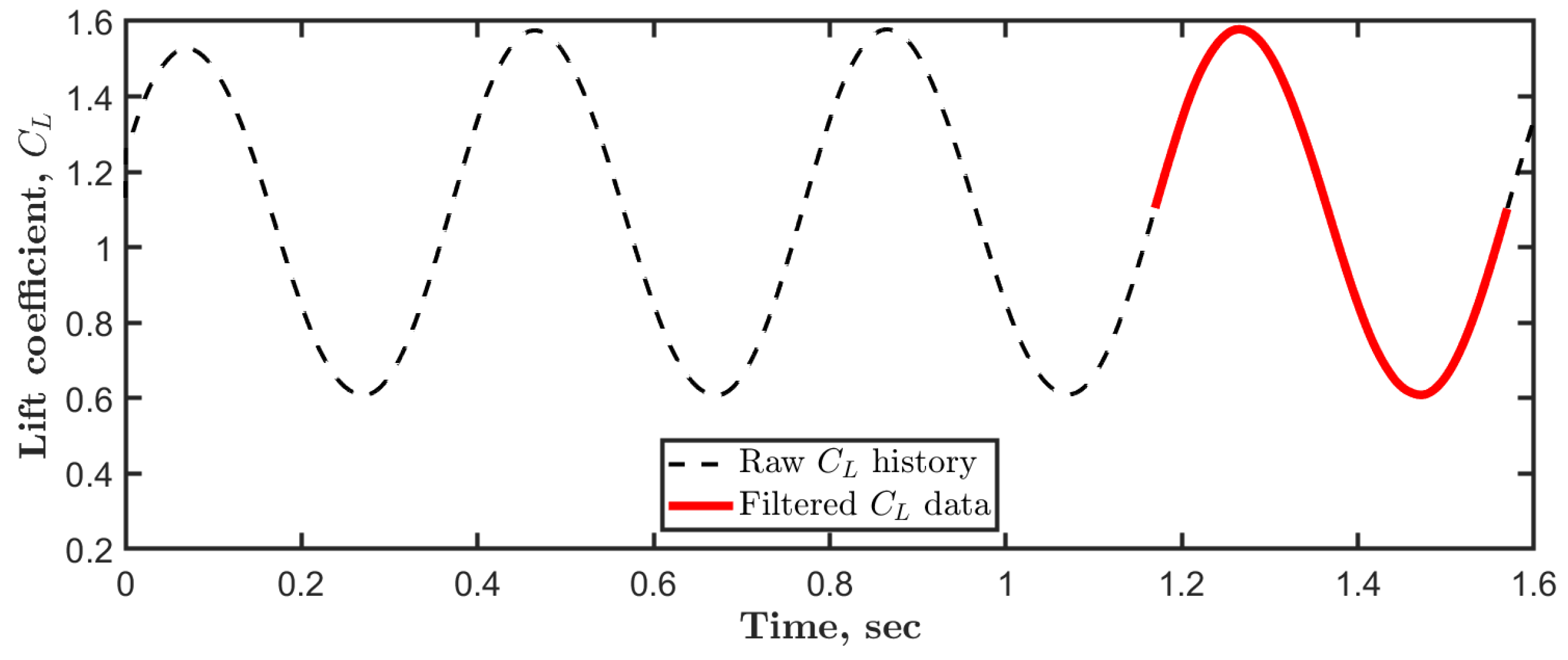
The raw data collected during the simulations include a wide range of unsteady aerodynamic forces and moments generated by the motion around each principal axis. These records capture the oscillatory response of aircraft aerodynamic performance to the prescribed harmonic motions. In order to filter the results, the initial cycles are excluded, and attention is focused on the last oscillation cycle. This filtering step is carried out to eliminate data from the initial transient phase, which would provide not yet fully converged behavior. Then, the aerodynamic data are analyzed to extract the dynamic stability derivatives by relating the aerodynamic coefficients to their corresponding kinematic inputs, such as angular displacements and angular rates. Basically, the dynamic stability derivatives can be determined by evaluating the slopes and trends in the aerodynamic coefficients relative to the imposed simple oscillations.

Following a commonly used procedure for the prediction of stability derivatives for complex configurations, the generic aerodynamic coefficient can be expressed as $C_j=C_j(\varphi ,\theta ,\psi ,p,q,r)$, where ($p,q,r$) are the rolling, pitching, and yawing rates, respectively. In this way, the linear approximation for the coefficient variation reads as has been defined in, e.g., [20]:

$$\begin{array}{cc}\hfill C_j-C_{j_0}& ={\displaystyle \frac{\partial C_j}{\partial \varphi }}(sin{\alpha }_0)\varphi +{\displaystyle \frac{\partial C_j}{\partial \theta }}\theta -{\displaystyle \frac{\partial C_j}{\partial \psi }}(cos{\alpha }_0)\psi \hfill \\ \hfill & +\left({\displaystyle \frac{\partial C_j}{\partial p}}+{\displaystyle \frac{\partial C_j}{\partial \dot{\varphi }}}sin{\alpha }_0\right)\dot{\varphi }+\left({\displaystyle \frac{\partial C_j}{\partial q}}+{\displaystyle \frac{\partial C_j}{\partial \dot{\theta }}}\right)\dot{\theta }+\left({\displaystyle \frac{\partial C_j}{\partial r}}-{\displaystyle \frac{\partial C_j}{\partial \dot{\psi }}}cos{\alpha }_0\right)\dot{\psi },\hfill \end{array}$$

(1)

with ${\alpha }_0$ representing the initial AoA. By imposing a rolling SHO (around the X axis), the above expression becomes

$$C_j-C_{j_0}=C_{j_{\varphi }}(sin{\alpha }_0)\varphi +\left(C_{j_p}+C_{j_{\dot{\varphi }}}sin{\alpha }_0\right)\dot{\varphi },$$

(2)

where the derivatives are denoted as $C_{j_{\varphi }}\equiv {\displaystyle \frac{\partial C_j}{\partial \varphi }}$, $C_{j_p}\equiv {\displaystyle \frac{\partial C_j}{\partial p}}$, and $C_{j_{\dot{\varphi }}}\equiv {\displaystyle \frac{\partial C_j}{\partial \dot{\varphi }}}$. Analogously, for a pitching SHO (around the Y axis), one has

$$C_j-C_{j_0}=C_{j_{\theta }}\theta +\left(C_{j_q}+C_{j_{\dot{\theta }}}\right)\dot{\theta },$$

(3)

while, for a yawing SHO (around the Z axis), one has

$$C_j-C_{j_0}=-C_{j_{\psi }}(cos{\alpha }_0)\psi +\left(C_{j_r}-C_{j_{\dot{\psi }}}cos{\alpha }_0\right)\dot{\psi }.$$

(4)

In the present study, the above expressions were actually written for the aerodynamic coefficients $C_l$, $C_m$, and $C_n$, associated with the moment components illustrated in Figure 2. The direct and cross derivatives that appear in the corresponding Equations (2)–(4) are summarized in

Table 2. Dynamic derivatives of moment coefficients determined through SHO motions.

Motion	Direct Derivatives	Cross-Derivatives
Rolling	$C_{l_{\varphi }}$, $C_{l_p}+C_{l_{\dot{\varphi }}}$$sin{\alpha }_0$	$C_{n_{\varphi }},C_{n_p}+C_{n_{\dot{\varphi }}}$$sin{\alpha }_0$
Pitching	$C_{m_{\theta }}$, $C_{m_q}+C_{m_{\dot{\theta }}}$	–
Yawing	$C_{n_{\psi }}$, $C_{n_r}-C_{n_{\dot{\psi }}}$$cos{\alpha }_0$	$C_{l_{\psi }}$, $C_{l_r}-C_{l_{\dot{\psi }}}$$cos{\alpha }_0$

. Notably, beside the normal coefficients, $C_{l_{\varphi }}$, $C_{m_{\theta }}$, and $C_{n_{\psi }}$, as well as the cross derivatives, $C_{n_{\varphi }}$ and $C_{l_{\psi }}$, the other dynamic stability parameters consist of coupled terms representing the simultaneous dependence on both oscillation rates and time rates of change of corresponding angular positions.

The evaluation of the various dynamic stability derivatives can be attained by exploiting the unsteady numerical data provided by the CFD simulations. The practical procedure leads to the solution of a least squares problem, where the dependent variables are the integrated aerodynamic coefficients, while the independent arguments are the instantaneous oscillation angles and their rates of change [6]. The interested reader is referred to the cited references for a detailed description of the method.

3. Computational Model

3.1. Aircraft Model

This study leverages the NASA CRM as the reference aircraft geometry [21]. This particular model features a high-aspect-ratio wing with a moderately swept leading edge, which is optimized for efficient performance at transonic cruise conditions. It also includes a horizontal tailplane designed to ensure stability and control, as well as a fuselage whose proportions are representative of a typical commercial aircraft. While the original CRM configuration incorporates nacelles and pylons to account for engine installation effects, these components were excluded in the present study to simplify the computational test cases for CFD analyses. In fact, herein, the focus remains on the aerodynamic characteristics of the clean airframe, minimizing the complexities introduced by propulsion-related elements. The CRM in its Wing-Body-Tail (WBT) configuration is shown in Figure 3. Key geometric parameters of the present flight vehicle model, such as mean aerodynamic chord (MAC), wing span, reference surface area, fuselage length, and aspect ratio (AR), are summarized in

Table 3. NASA CRM: reference parameters.

Parameter	Symbol	Value	Unit
MAC	cref	7	m
Wing Span	b	58.8	m
Reference Surface	Aref	383.7	m2
Fuselage Length	lfus	62.79	m
Aspect Ratio	AR	9.0	-

.

3.2. Numerical Method

This section summarizes the numerical setup implemented to accurately simulate unsteady aerodynamics effects during simple aircraft maneuvers, including the grid generation, the CFD solver settings, and the dynamic meshing technique.

3.2.1. Grid Generation

To perform the present CFD analysis, a computer-aided design (CAD) geometry of the NASA CRM was treated by using the advanced BETA CAE pre-processing software ANSA v24.1.0 [22], where a combination of different meshing techniques was employed for discretizing the computational domain. First, the surface mesh on the aircraft body was generated by using both triangular and square elements. This surface mesh was then extended into an anisotropic hexahedral volume mesh, incorporating structured prismatic layers to capture boundary layer effects. Figure 4 illustrates the surface mesh, the volume mesh, and the boundary layer mesh, with localized refinements applied at the leading and trailing edges of the aircraft wing. In order to perform a grid convergence analysis, a set of three progressively optimized unstructured hybrid grids was employed.

Table 4. Grid convergence analysis: mesh parameters for varying spatial resolution.

Resolution	Cells Number	Leading Edge Spacing	Wall-Normal Spacing	${\mathit{y}}^{+}$
Coarse	8.6 M	0.013 m	$2.4\times {10}^{-3}$ m	10
Medium	10.2 M	0.011 m	$2.4\times {10}^{-4}$ m	1
Fine	11.0 M	0.0097 m	$2.4\times {10}^{-5}$ m	0.2

provides details about the grid resolution levels that were employed (referred to as coarse, medium, and fine). In this table, the total number of computational cells is reported, along with a couple of parameters describing the spatial resolution on the main wing, namely, the linear extent of the refined surface elements in the leading edge region, and the first mesh spacing in the wall-normal direction. The corresponding nondimensional $y^{+}$ value, determining the accuracy of the boundary layer prediction, is also provided.

3.2.2. CFD Solver Settings

Following previous studies [23,24], the simulations were conducted using a “free-air” setup, avoiding the influence of wind tunnel walls or model support structures. The outer boundary of the computational domain had a spherical shape, with a radius of 500 m, where far-field boundary conditions, based on Riemann invariants, were applied. The aircraft surfaces were treated as adiabatic no-slip walls. The free-stream airflow conditions were characterized by the temperature $T_{\mathrm{ref}}=310$ K, pressure $p_{\mathrm{ref}}=$ 101,325 Pa, and velocity $V_{ref}=300$ m/s. Correspondingly, the flight Reynolds number, based on the MAC, and the Mach number resulted in being $Re=5\times {10}^6$ and $Ma=0.85$, respectively.

The compressible RANS governing equations were solved using ANSYS Fluent 2024 R2. A cell-centered finite volume method was employed, with fluxes at the cell faces calculated using the Roe scheme. A pressure-based, fully coupled algorithm was utilized, employing second-order upwind schemes for the discretization of convective and diffusive fluxes. Additionally, the least-squares cell-based method was applied for gradient computation. The resulting system of linear equations was solved using a point-implicit Gauss–Seidel method, in conjunction with an algebraic multigrid solver. Turbulence modeling was addressed using the shear stress transport (SST) k-$\omega$ turbulence closure model [25], which is commonly used in applied computational aerodynamics, e.g., [23]. For the initial verification study, the target characteristics were grid-converged values for the lift, drag, and pitching moment coefficients.

As far as transient simulations are concerned, a time step of $\Delta t=5\times {10}^{-4}\mathrm{s}$ was selected to ensure the convergence and stability of the calculations, similarly to [26], where a time step of $\Delta t\approx 0.006\mathrm{s}$ was employed. This way, the cell convective Courant number was practically maintained of the order unity around the aircraft surfaces. Also, to guarantee convergence of the normalized residuals, twenty iterations for the inner loop were performed at each time step during the time integration.

3.2.3. Dynamic Meshing

In the current applied CFD framework, a transient analysis was performed by utilizing the dynamic mesh technique, e.g., [27]. This approach allows one to continuously modify the shape of the computational domain during the ongoing simulation by moving boundaries or particular zones while either deforming or adding/removing cells. Unlike the sliding mesh method, which is used for rigid body motion between predefined mesh zones, such as rotating machinery, the current dynamic mesh technique is suited for cases where the computational domain undergoes continuous deformation, requiring mesh updates via smoothing, remeshing, or layering.

Practically, a smaller spherical subdomain is created enclosing the aircraft model. This sphere, which has a radius of 100 m, moves rigidly with the surface and boundary layer meshes, while the outer subdomain remains stationary relative to the far field. Figure 5 shows the dynamic meshing setup, featuring the smaller inner sphere nested within a larger outer one. The area between the two regions constitutes the dynamic mesh zone, as shown in Figure 6, where mesh updates occur via smoothing at each temporal increment. This ensures that dynamic mesh interactions, such as updates and smoothing, occur far from the fine prism boundary layer surrounding the model’s surface. The larger and more uniform elements in the outer region require fewer updates and are easier to be deformed during motion, leading to lower computational cost. Indeed, larger elements reduce the number of nodes involved in mesh smoothing and remeshing algorithms. This arrangement lowers the computational load and complexity of each mesh update, helping to avoid issues related to skewed or negative mesh volumes during the smoothing process and therefore improving the stability and efficiency of the dynamic procedure.

Notably, the dynamic mesh configuration allows for more precise handling of the boundary layer flow around the aircraft model, which is crucial for the accurate prediction of aerodynamic forces, particularly in high-fidelity simulations, where the movement of the model can induce non-negligible flow-field changes. By avoiding excessive mesh deformation near the model, the method ensures that crucial flow features, such as separation and vortex formation, are accurately captured without introducing numerical errors.

In the framework of the CFD software package, the dynamic meshing technique was practically configured through ad hoc coded UDF procedures employing the macro DEFINE_CG_MOTION for specifying the motion of the prescribed dynamic subdomain [28]. These functions determine the components for both translational and angular velocities. Here, three different UDFs were used to represent three distinct modes of simple harmonic oscillation, with no translational velocity. For instance, in the first UDF, the model’s pitching motion is achieved by applying a sinusoidal rotation around the Y axis. This approach offers significant flexibility, as it allows for the specification of customizable oscillatory motion profiles tailored to the specific needs of the desired analysis. By defining rotational motions with constant angular velocities for pitching, rolling, and yawing, the current technique is able to reproduce dynamic effects like pitching or rolling instabilities. Moreover, the ability to fine-tune these motions opens up possibilities for investigating a wide range of aerodynamic phenomena, thus broadening the scope of the dynamic mesh technique’s applications in aircraft stability and control studies. This versatility makes the dynamic meshing approach particularly powerful in capturing the transient behavior of complex aerodynamic systems under various flight conditions.

4. Results and Discussion

In this section, after providing the preliminary results for static simulations, conducted for varying AoAs, the three different dynamic analyses performed are presented and discussed.

4.1. Static Case Validation

To evaluate the static aerodynamic characteristics of the aircraft model, we began by analyzing its behavior for varying AoAs ($\alpha$ in the following description). First of all, a grid convergence study was carried out to determine the proper mesh resolution. Three coarsening levels of unstructured grids were utilized, as described in Section 3.2.1. These initial simulations also served the purpose of estimating the static aerodynamic characteristics of the aircraft model under study. The static state was studied at the free-stream Mach number $0.85$, for $0^{\circ }<\alpha <{18}^{\circ }$, and the sideslip angle $\beta =0$°. Practically, steady RANS simulations were carried out by employing the three different grids summarized in Table 4. In this case, to take advantage of the expected flow symmetry, only half the computational model represented in Figure 5 was actually employed in the simulations, where the flow symmetry boundary condition was imposed at the plane $Y=0$.

Figure 7 displays the aerodynamic force coefficients for varying AoAs obtained for the three different static mesh resolutions. The present results were compared against reference data from both experimental [29] and numerical [30] works. Specifically, Figure 7a shows the increasing lift coefficient versus the AoA, while the drag polar is reported in Figure 7b. Moreover, the pitching moment coefficient is reported in Figure 7c. Overall, the agreement between present converged results and reference data is quite good. Notably, the current solutions suggest a higher (positive) pitching moment (nose-up) for a given lift coefficient when compared to experiment. This discrepancy may partially stem from the absence of corrections for the mounting system in the experimental data. Additionally, it is important to note that at higher AoAs, the wind tunnel model experienced significant buffeting due to increased flow separation and shock movement. Following [31], some unsteady phenomena observed at higher AoAs were not captured by the test data, nor were they reproduced by CFD simulations.

Furthermore, the pressure distributions at two different main wing sections were considered for a particular AoA of $\alpha =4^{\circ }$. The two sections selected are representative of inboard and outboard regions of the wing, as illustrated in Figure 8. Here, the normalized section location is individuated by $\eta =Y/(b/2)$, where Y represents the wing section position, and b stands for the wing span length. The current sections correspond to the spanwise locations $\eta \cong 0.502$ and $0.727$, respectively. Figure 9 shows the corresponding pressure distributions for varying numerical resolutions compared to reference experimental data in [31] obtained at the same Mach and Reynolds numbers.

Apparently, at the inboard section (Figure 9a), the pressure coefficient showed a smooth variation along the chord length. The different numerical results closely match, especially in the leading edge region, where a significant pressure drop was observed. For the outboard section (Figure 9b), the pressure distribution appears more complex, due to the influence of strong three-dimensional effects and flow separation. Discrepancies observed for the shock location on the suction side of the wing may be attributed to either mesh density, as already noticed by Sclafani et al. [30], or the turbulence model employed. Overall, the results presented show that the grids employed led to acceptably accurate results. The medium mesh was chosen for the dynamic simulations discussed in the following in order to balance accuracy of the numerical simulations and computational cost.

4.2. Dynamic Stability Derivatives Analysis

This section presents the results derived from various transient simulations, which were used to analyze the dynamic stability derivatives of the CRM along its rotational axes. The derivatives are related to independent motion variables that are $\varphi$, $\theta$, and $\psi$, as well as $\dot{\varphi }$, $\dot{\theta }$, and $\dot{\psi }$. These parameters characterize the response of the aircraft to simple motions and indicate its ability to regain equilibrium after being disturbed, providing insights into the dynamic stability of the aircraft.

In this study, the dynamic stability derivatives were computed by applying disturbances in the form of sinusoidal oscillatory motions to the aircraft model, in its full configuration, about its center of gravity. For all pitching, yawing, and rolling motions, the oscillation frequency $f=2.5$ Hz was selected, for which $\omega =15.7$ rad/s denotes the corresponding angular velocity.

4.2.1. Pitching Oscillation

To determine the dynamic stability derivatives around the pitch axis, the aircraft model was subjected to a sinusoidal pitching motion. The kinematic relationships for the pitch angle and pitching rate for a harmonic pitching motion are defined as follows [26]:

$$\begin{array}{cc}\hfill \theta \left(t\right)& =\alpha \left(t\right)-{\alpha }_0={\theta }_{A}sin\left(\omega t\right),\hfill \\ \hfill \dot{\theta }& =\dot{\alpha }=q=\omega {\theta }_{A}cos\left(\omega t\right),\hfill \\ \hfill \ddot{\theta }& =\ddot{\alpha }=\dot{q}=-{\omega }^2{\theta }_{A}sin\left(\omega t\right),\hfill \end{array}$$

(5)

where ${\alpha }_0$ represents the initial AoA, and ${\theta }_A$ is the maximum oscillation angle. For the present calculations, these parameters were prescribed as either ${\alpha }_0={10}^{\circ }$ or ${\alpha }_0={15}^{\circ }$ and ${\theta }_A=5^{\circ }$, respectively. Also, the constant roll and yaw angles remained fixed at ${\varphi }_0=0^{\circ }$ and ${\psi }_0=0^{\circ }$, respectively. The time histories of the AoA and pitch rate are reported in Figure 10, where the last cycle is considered to filter the results. For the lift coefficient, for instance, the comparison between the different cycles and the filtered data is illustrated in Figure 11. This filtering process was essential to exclude the transient region data, which did not yet fully converge during the initial cycles.

Figure 12 presents the plots of the unsteady lift and pitching moment coefficients for the pitching oscillation cycles corresponding to both initial AoAs. The trends of both $C_L$ and $C_m$ against $\theta$ are consistent with previous research findings, e.g., [32]. In the transonic regime, the plot of $C_L$ against $\theta$ typically shows a nearly linear increase for small pitch angles. However, owing to the relatively high Mach number, a more pronounced hysteresis loop may be observed. This phenomenon occurs because shock waves can form and move over the wing surface, altering the local pressure distribution and delaying flow separation, which significantly affects the lift characteristics. The hysteresis loop observed for the lift coefficient as a function of $\theta$ during sinusoidal pitching oscillations is expected to be more significant due to the interaction between shock waves and boundary layers. Indeed, this interaction can cause flow separation and reattachment, leading to a complex aerodynamic response [33]. The loop shows a positive slope for increasing values of $\theta$, appearing to be centered around $\theta =0^{\circ }$, suggesting balanced aerodynamic behavior. This symmetry indicates that the aircraft responds similarly during both the increasing and decreasing phases of AoA, which is a sign of good dynamic stability. This fact suggests that the aircraft is capable of returning to equilibrium after a small disturbance, which is a critical characteristic of dynamic stability. When comparing the results for the two different initial AoAs, marked differences in aerodynamic behavior are observed. At ${\alpha }_0={15}^{\circ }$, the aircraft operated closer to the stall boundary, resulting in a more pronounced hysteresis loop in the $C_L$ vs. $\theta$ plot. The increased AoA intensified the effects of shock waves and flow separation, which in turn led to more complex and nonlinear lift behavior. In contrast, at ${\alpha }_0={10}^{\circ }$, the response of the aircraft remained more stable and linear, since it operated far from the stall regime. The reduced impact of shock waves and flow separation results in less hysteresis in the lift coefficient, allowing for a more predictable flow behavior, thus indicating an improved overall dynamic stability.

The plot of $C_m$ against $\theta$ provides insight into the longitudinal stability of the aircraft. In the transonic regime, shock waves can induce abrupt changes in the pitching moment, leading to potential nonlinearities. The trim point, where $C_m$ is zero, may shift due to compressible flow and shock wave interactions. This shift indicates that the aircraft equilibrium position varies with flight conditions, which represents an important factor for stability and control. Again, the variation in $C_m$ is more pronounced at higher initial AoAs, where stronger shock wave interactions and flow separation can destabilize the equilibrium, whereas the pitching moment remains more stable at lower initial AoAs. These findings highlight the significant role of the initial AoA in determining the stability characteristics of the aircraft, as it directly influences the response of the pitching moment and consequently the overall stability of the system.

The dynamic stability derivatives evaluated through the pitching SHO motion, for the two different initial AoAs, are summarized in

Table 5. Dynamic stability derivatives determined through pitching SHO motion for varying initial AoAs.

${\mathit{\alpha }}_0$ [deg]	${\mathit{C}}_{{\mathit{m}}_{\mathit{\theta }}}$ [deg−1]	$({\mathit{C}}_{{\mathit{m}}_{\mathit{q}}}+{\mathit{C}}_{{\mathit{m}}_{\dot{\mathit{\theta }}}})$ [s · deg−1]
10	−0.054	−0.765
15	−0.058	−0.772

. It is worth noting that, due to the imposed harmonic oscillation, the pitching rate q coincides with the time rate of change of the angle $\theta =\alpha -{\alpha }_0$ (5). Nevertheless, the coefficients $C_{m_q}$ and $C_{m_{\dot{\theta }}}$ can be theoretically assumed as separate parameters while practically estimating the summed coefficient ($C_{m_q}+C_{m_{\dot{\theta }}}$) appearing in the corresponding linear approximation (3), e.g., [20]. This is perfectly consistent with the usual procedure employed for the evaluation of dynamic stability derivatives using CFD data, e.g., [6,26]. A similar argument can be made for the coefficients $C_{j_p}$ and $C_{j_{\dot{\varphi }}}$, as well as for $C_{j_r}$ and $C_{j_{\dot{\psi }}}$, in the following discussions concerning rolling and yawing harmonic oscillations, respectively.

Apparently, looking at the values for the derivative $C_{m_{\theta }}$, an increase in the pitch angle produces a negative pitching moment, which contributes to the longitudinal stability of the aircraft, and this property is maintained for varying AoA. Similarly, the observed values for the coupled coefficient $(C_{m_q}+C_{m_{\dot{\theta }}})$ show that a positive variation in the pitching rate also produces a negative variation of the pitching moment, again granting stability. These results demonstrate that the aircraft model maintains good longitudinal dynamic stability. Also, the slight modification in the derivative values suggests that a change in the initial AoA has little impact on the overall stability of the CRM under study.

4.2.2. Rolling Oscillation

In order to determine the dynamic stability derivatives for the rolling motion, the aircraft was subjected to sinusoidal oscillations around the roll axis. The kinematic relationships for the roll angle and rolling rate during a harmonic rolling motion are defined as follows [26]:

$$\begin{array}{cc}\hfill \varphi \left(t\right)-{\varphi }_0& ={\varphi }_{A}sin\left(\omega t\right),\hfill \\ \hfill \dot{\varphi }& =p=\omega {\varphi }_{A}cos\left(\omega t\right),\hfill \\ \hfill \ddot{\varphi }& =\dot{p}=-{\omega }^2{\varphi }_{A}sin\left(\omega t\right),\hfill \end{array}$$

(6)

where ${\varphi }_0$ represents the mean value, and ${\varphi }_A$ is the maximum oscillation angle. Here, these parameters were set to ${\varphi }_0=0^{\circ }$, and ${\varphi }_A=5^{\circ }$. Moreover, the constant pitch and sideslip angles were set to either ${\alpha }_0={10}^{\circ }$ or ${\alpha }_0={15}^{\circ }$ and ${\beta }_0=0^{\circ }$, respectively.

Figure 13 presents the trends of the lateral force coefficient ($C_Y$), the rolling moment coefficient ($C_l$), and the yawing moment coefficient ($C_n$) as a function of varying the roll angle $\varphi$ for both initial AoAs. The coefficient $C_Y$ increases with $\varphi$, with the relationship being generally linear for small roll angles. As the roll angle increases, the lateral force generated by the fuselage also increases, resulting in a positive slope in the $C_Y$ vs. $\varphi$ plot, as in the absence of a vertical tail [34].

When comparing the results achieved for the two different initial AoAs, marked differences in the behavior of $C_Y$ become evident, although the changes are more subtle than for other aerodynamic coefficients. For ${\alpha }_0={10}^{\circ }$, the aircraft exhibits a relatively stable lateral force response, with $C_Y$ increasing predictably and nearly linearly with the roll angle. Since the aircraft is operating further from the stall boundary, the flow remains stable, and the lateral force distribution is consistent and well behaved. This results in a more linear relationship between the lateral force coefficient and the roll angle $\varphi$. In contrast, for ${\alpha }_0={15}^{\circ }$, the $C_Y$ plot remains symmetric, but it shows a slight deviation from an ideal elliptical path as the roll angle increases. This subtle deviation from the idealized behavior emphasizes the importance of compressible flow at higher AoAs. While the aircraft is still far from the stall boundary, these effects start to manifest more noticeably, leading to slight nonlinearities in the lateral force response, which could influence the overall dynamic stability of the aircraft.

As to the coefficient $C_l$, it is influenced by the dihedral effect and the wing configuration. For a positive roll angle, the aircraft tends to roll in the opposite direction due to the differential lift on the wings. This results in a negative slope in the $C_l$ vs. $\varphi$ plot. The dihedral effect, which stabilizes the aircraft during the rolling motion, is a key factor in generating this negative slope. In the transonic flow regime, shock wave and boundary layer interactions can introduce oscillations or hysteresis in the $C_l$ vs. $\varphi$ plot, leading to nonlinearities that complicate the analysis of the aircraft roll stability. In particular, for ${\alpha }_0={10}^{\circ }$, the relationship between $C_l$ and the roll angle remained relatively smooth and symmetric, reflecting a more stable aerodynamic behaviour of the aircraft. Indeed, the rolling moment curve follows a predictable elliptical path, indicating that the aircraft response is well-behaved and the dynamics are stable. In contrast, for ${\alpha }_0={15}^{\circ }$, the rolling moment coefficient deviated from an idealized elliptical path. The trajectory of $C_l$ became nonlinear, indicating a stronger influence of shock waves and flow separation. In this case, the aerodynamic response becomes more complex and less predictable.

The coefficient $C_n$ showed a negative slope with respect to $\varphi$, leading to the observed directional stability. For ${\alpha }_0={10}^{\circ }$, the $C_n$ curve remained relatively smooth and symmetric, reflecting a stable and predictable yawing moment response. However, in the transonic regime, the presence of shock waves can cause abrupt changes in the yawing moment, potentially leading to nonlinearities in the corresponding plot. This behavior is indicative of complex shock–boundary layer interactions that can alter the aircraft directional response during roll oscillations. Moreover, for ${\alpha }_0={15}^{\circ }$, the $C_n$ curve shows a positive slope, remains symmetric but deviates from the ideal elliptical path. This deviation suggests that at higher AoAs, the directional stability becomes less predictable, and the yawing moment response exhibits slight asymmetries. These nonlinearities in the yawing moment could result in a temporary loss of the restoring moment, which might affect the overall stability of the aircraft.

Table 6. Dynamic stability derivatives determined through rolling SHO motion for varying initial AoAs.

${\mathit{\alpha }}_0$ [deg]	${\mathit{C}}_{{\mathit{l}}_{\mathit{\varphi }}}$ [deg−1]	$({\mathit{C}}_{{\mathit{l}}_{\mathit{p}}}+{\mathit{C}}_{{\mathit{l}}_{\dot{\mathit{\varphi }}}}$$sin{\mathit{\alpha }}_0)$ [s · deg−1]	${\mathit{C}}_{{\mathit{n}}_{\mathit{\varphi }}}$ [deg−1]	$({\mathit{C}}_{{\mathit{n}}_{\mathit{p}}}+{\mathit{C}}_{{\mathit{n}}_{\dot{\mathit{\varphi }}}}$$sin{\mathit{\alpha }}_0)$ [s · deg−1]
10	−0.0502	0.0438	−0.0571	−0.0021
15	−0.1331	0.0372	0.0501	−0.0004

reports the dynamic stability derivatives determined through the rolling SHO motion for the two different initial AoAs. The observed negative values of $C_{l_{\varphi }}$ demonstrate a stabilizing dihedral effect [35], while the positive values of the coefficient $(C_{l_p}+C_{l_{\dot{\varphi }}}$$sin{\alpha }_0)$, representing negative roll damping, reflect an enhancement effect on the roll response. The dihedral effect increases with the AoA, which stabilizes the aircraft more effectively during the rolling motion. In contrast, the damping effect is slightly reduced at higher AoA, which is likely due to the increased influence of shock waves and flow separation at higher incidences, leading to a more complex (and less predictable) aerodynamic response. Looking at the cross-derivatives, the slightly negative value of $C_{n_{\varphi }}$ at lower AoA suggests that the aircraft tends to yaw in the opposite direction of the applied roll angle, contributing to a stable yawing moment response. Differently, at higher AoA, the same derivative results in being positive, with the hysteresis loop deviating from the ideal elliptical path. In fact, the directional stability becomes less predictable, and the yawing moment response exhibits slight asymmetries. These nonlinearities in the yawing moment could also result in a temporary loss of the restoring moment, potentially affecting the overall stability of the aircraft. Notably, the damping effect associated with the coupled coefficient ($C_{n_p}+C_{n_{\dot{\varphi }}}$$sin{\alpha }_0$) becomes practically negligible at higher AoA.

4.2.3. Yawing Oscillation

Dynamic stability derivatives around the yaw axis were evaluated by subjecting the aircraft to sinusoidal yawing oscillations. The kinematic relationships for the yaw angle and yawing rate during a harmonic yawing motion are defined as follows [26]:

$$\begin{array}{cc}\hfill \psi \left(t\right)& =-\beta \left(t\right)+{\beta }_0={\psi }_{A}sin\left(\omega t\right),\hfill \\ \hfill \dot{\psi }& =-\dot{\beta }=r=\omega {\psi }_{A}cos\left(\omega t\right),\hfill \\ \hfill \ddot{\psi }& =-\ddot{\beta }=\dot{r}=-{\omega }^2{\psi }_{A}sin\left(\omega t\right),\hfill \end{array}$$

(7)

where ${\beta }_0$ represents the mean sideslip angle, and ${\psi }_A$ is the maximum oscillation angle. In the present calculations, these parameters were set to ${\beta }_0=0^{\circ }$, and ${\psi }_A=5^{\circ }$. Also, the constant pitch and roll angles were fixed at either ${\alpha }_0={10}^{\circ }$ or ${\alpha }_0={15}^{\circ }$ and ${\varphi }_0=0^{\circ }$, respectively.

Figure 14 presents the time histories of $C_Y$, $C_l$, and $C_n$ coefficients as a function of the yaw angle $\psi$ for both initial AoAs. The lateral force coefficient $C_Y$ shows a linear variation, while the $C_Y$ curve exhibits a negative slope, indicating a restoring lateral force that opposes the yawing motion. This restoring force is crucial for maintaining dynamic stability around the yaw axis, as it acts to return the aircraft to its equilibrium position when the yaw angle deviates from zero. For ${\alpha }_0={10}^{\circ }$, the curve follows an elliptical trend, suggesting a consistent and predictable relationship between the yaw angle and the lateral force. For ${\alpha }_0={15}^{\circ }$, the curve remains symmetric with a negative slope, but it deviates from the elliptical shape, indicating nonlinearity in the aerodynamic response. This deviation is likely due to the onset of shock waves or flow separation, which affect the aircraft stability at higher AoAs.

Furthermore, during a yaw rotation, the asymmetric distribution of aerodynamic forces on the wings generates a rolling moment. The sign and magnitude of $C_l$ depend on both the direction and amplitude of the yaw oscillation. For sinusoidal excitations, the rolling moment coefficient typically follows an elliptical pattern, reflecting a phase difference between the yawing motion and the resulting rolling moment. This phase difference is essential for understanding the dynamic stability of the aircraft, as it provides insight into the coupling between yaw and roll responses [34]. Both curves obtained for different AoAs show an elliptical trend with a positive slope, signifying that the rolling moment acts in the direction of the yawing motion, contributing to the dynamic stability of the aircraft. Basically, the positive slope suggests that the aircraft will naturally counteract yaw disturbances by inducing a rolling moment that helps restore equilibrium. The larger $C_l$ values at ${\alpha }_0={15}^{\circ }$ suggest a more pronounced roll response, which can be advantageous for maintaining stability during larger yaw oscillations, but also indicates an increased sensitivity to yaw disturbances. The elliptical pattern of $C_l$ emphasizes the importance of yaw–roll coupling in assessing the overall stability of the aircraft. Actually, the phase difference between yawing and rolling moments is crucial for ensuring the aircraft can return to stable flight after disturbances.

The coefficient $C_n$ exhibits a negative slope during sinusoidal yaw rotation, indicating good directional stability for both initial AoAs. This behavior suggests that the aircraft experiences a counteracting yawing moment, which helps restore equilibrium after a yaw disturbance. Indeed, such a restoring force is crucial for maintaining stability around the yaw axis. The values of $C_n$ increase with the AoA, reflecting a stronger yawing moment and more pronounced response to yaw disturbances. For ${\alpha }_0={10}^{\circ }$, the curve takes an elliptical shape, indicating a linear and predictable system response. In contrast, for ${\alpha }_0={15}^{\circ }$, the curve retains its negative slope but deviates from the elliptical pattern, revealing the emergence of nonlinearity. The latter condition may be attributed to complex aerodynamic effects, such as compressible flow separation and increased shock wave interactions, which become more prominent at higher AoAs. These effects can alter the damping behavior, reducing the effectiveness of the restoring force and leading to a less predictable yaw response. This fact implies a more complex dynamic response. While the yawing moment continues to restore the aircraft to equilibrium, the presence of nonlinear effects suggests that the aircraft directional stability may be reduced, particularly under more extreme yaw disturbances.

As to quantitative evaluations, the dynamic stability derivatives determined through the yawing SHO motion are reported in

Table 7. Dynamic stability derivatives determined through yawing SHO motion for varying initial AoAs.

${\mathit{\alpha }}_0$ [deg]	${\mathit{C}}_{{\mathit{n}}_{\mathit{\psi }}}$ [deg−1]	$({\mathit{C}}_{{\mathit{n}}_{\mathit{r}}}-{\mathit{C}}_{{\mathit{n}}_{\dot{\mathit{\psi }}}}$$cos{\mathit{\alpha }}_0)$ [s · deg−1]	${\mathit{C}}_{{\mathit{l}}_{\mathit{\psi }}}$ [deg−1]	$({\mathit{C}}_{{\mathit{l}}_{\mathit{r}}}-{\mathit{C}}_{{\mathit{l}}_{\dot{\mathit{\psi }}}}$$cos{\mathit{\alpha }}_0)$ [s · deg−1]
10	−0.0259	−0.0128	0.0608	−0.0269
15	−0.0339	−0.0105	0.0815	−0.0254

for the two different initial AoAs. By inspection of direct derivatives, negative values of $C_{n_{\psi }}$ indicate that an increase in the yaw angle produces a restoring yawing moment. Similarly, negative values of the coefficient ($C_{n_r}-C_{n_{\dot{\psi }}}cos{\alpha }_0$) also suggest that an increase in the yawing rate produces a restoring yawing moment. Both facts contribute to demonstrating the directional stability of the aircraft, with the stable behavior being maintained for varying initial AoAs. In terms of the cross-derivatives, the positive values of $C_{l_{\psi }}$ indicate that the variation in the rolling moment acts in the direction of the yawing motion, contributing to dynamic stability. Practically, the aircraft model naturally counteracts yaw disturbances by inducing a rolling moment that helps restore equilibrium. The negative values of the coefficient ($C_{l_r}-C_{l_{\dot{\psi }}}$$cos{\alpha }_0$) reflect a damping effect on the rolling motion. At higher AoAs, the larger value of $C_{l_{\psi }}$ suggests a more pronounced roll response, which can be advantageous for maintaining stability during larger yaw oscillations. However, it also indicates an increased sensitivity to yaw disturbances. Moreover, the damping effect appears slightly reduced, which is likely due to the increased influence of shock waves and unsteady flow separation.

5. Conclusions

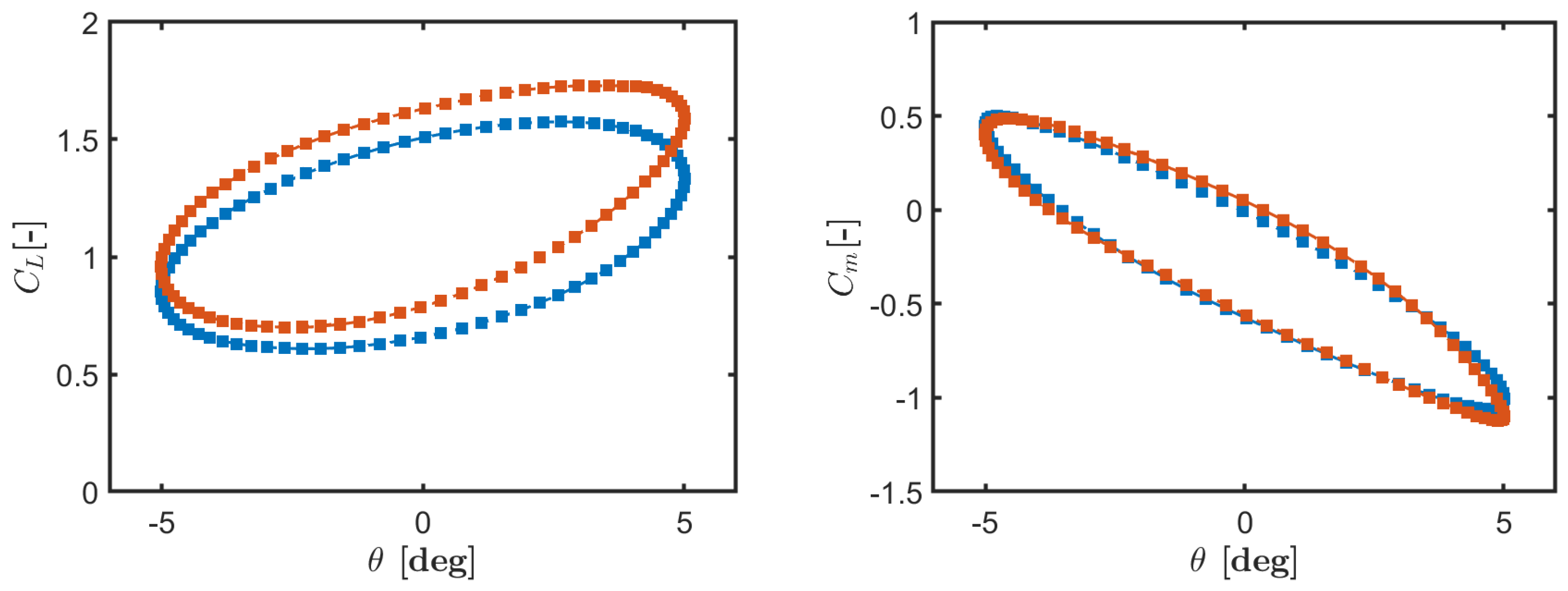
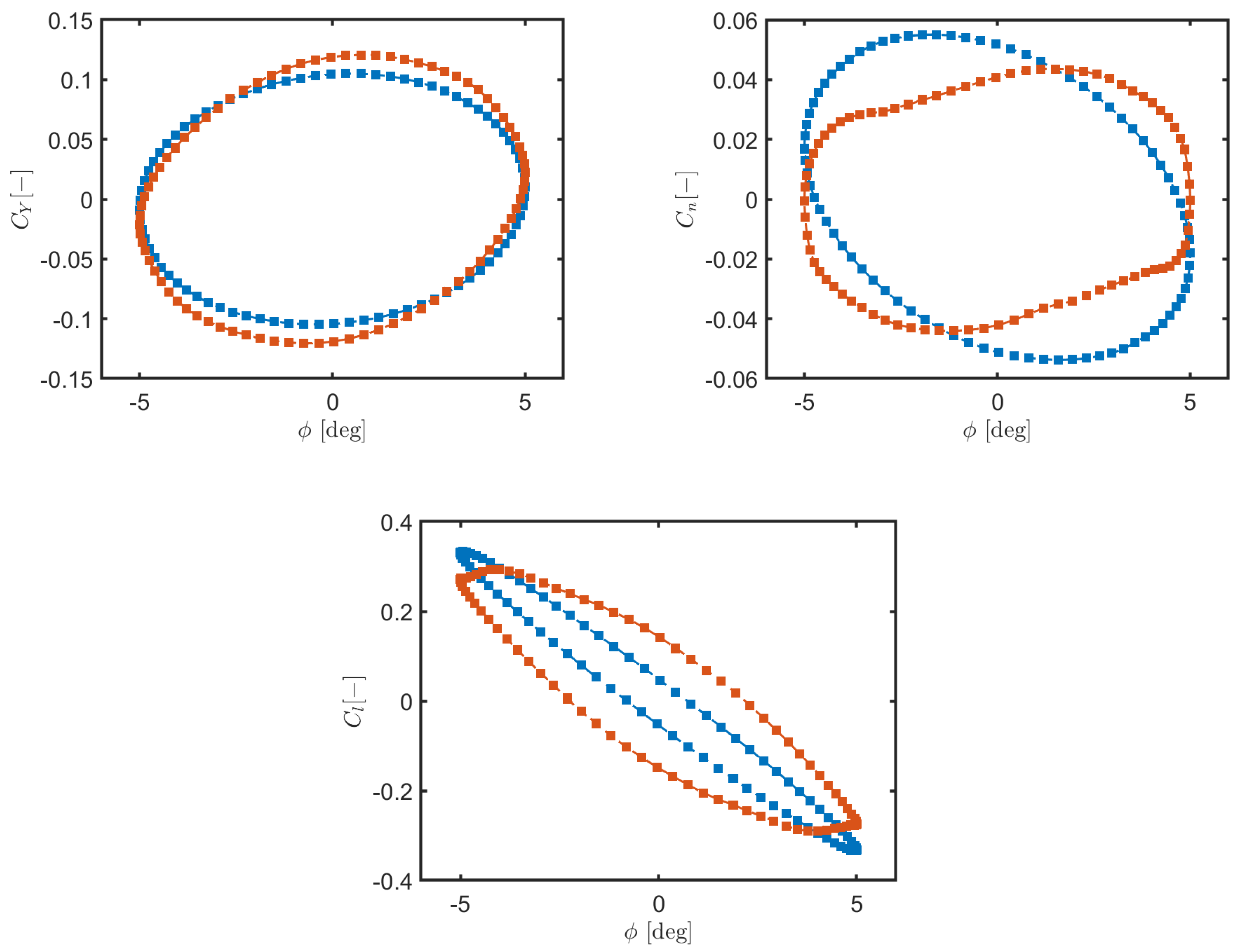
The work conducted in this study aimed to investigate the use of transient CFD simulations for evaluating the dynamic stability derivatives of commercial aircraft at feasible computational costs. Using the NASA common research model as a test case, the various computations demonstrated the effectiveness of the forced simple harmonic oscillation method in predicting dynamic derivatives across the various axes of motion (pitch, roll, and yaw). The results were obtained for a Reynolds number of $5\times {10}^6$ and a Mach number of $0.85$ for flight conditions that are representative of the transonic regime. As a proof of concept, dynamic stability derivatives were numerically evaluated and analyzed for two different flight conditions, corresponding to two different initial angles of attack.

A key finding of the present study was the effectiveness of dynamic meshing techniques in providing an accurate representation of unsteady aerodynamic behavior while maintaining computational efficiency. The unsteady aerodynamic coefficients allowed for a detailed evaluation of the longitudinal and lateral-directional stability of the aircraft, with particular attention to the complex effects introduced by compressible flow separations and shock-boundary layer interactions. Moreover, the current results confirmed that CFD-based forced oscillation methods can serve as a valuable alternative to traditional wind tunnel testing, providing greater flexibility in parametric studies and eliminating constraints related to test stand limitations [6,7]. The observed hysteresis effects in aerodynamic coefficient plots, particularly in the transonic regime, further underscore the importance of capturing nonlinear unsteady flow features, which are difficult to isolate in experimental setups. Moreover, this study demonstrated that the numerical approach aligns well with theoretical stability trends, reinforcing the reliability of CFD for stability derivative estimation. These findings suggest that CFD-based methods can be systematically integrated into early-stage aircraft design to refine aerodynamic performance predictions before physical testing, reducing development time and cost [1].

Overall, this study provided new insights into the dynamic behavior of the aircraft model in unsteady flow conditions, opening the path for future developments that could further improve aerodynamic design and flight performance simulation, particularly in transonic and supersonic regimes. In fact, while the present results are very promising, this study also highlighted areas for potential improvement. Specifically, to enhance the accuracy of the CFD simulations, future work will integrate higher-fidelity turbulence models, such as hybrid RANS-LES methods, which combine Reynolds-averaged Navier–Stokes (RANS) and large-eddy simulation (LES) approaches to better capture complex flow phenomena, as suggested by recent research findings, e.g., [36,37]. In addition, extending the current methodology to maneuvers involving coupled oscillations could provide deeper insights into cross-coupling aerodynamic effects, further testing the predictive capability of applied CFD models for aircraft stability analysis. Indeed, the scope of the research could be also expanded to more complex geometries, including engine nacelles and control surfaces, to better represent real-world flight conditions.

References

1. Mader, C.A.; Martins, J.R.R.A. Computation of aircraft stability derivatives using an automatic differentiation adjoint approach. AIAA J. 2011, 49, 2737–2750. [Google Scholar]
2. Ignatyev, D.I.; Khrabrov, A.N. Model of the unsteady aerodynamic characteristics at high AoA with nonlinear dependency in angular rate. In Proceedings of the 29th Congress of the Aeronautical Sciences, St. Petersburg, Russia, 7–12 September 2014. [Google Scholar]
3. Mi, B.; Zhan, H. Review of numerical simulations on aircraft dynamic stability derivatives. Arch. Comput. Methods Eng. 2020, 27, 1515–1544. [Google Scholar]
4. Davis, M.C.; White, J.T. X-43A flight-test-determined aerodynamic force and moment characteristics at Mach 7.0. J. Spacecr. Rocket. 2008, 45, 472–484. [Google Scholar]
5. Greenwell, D.I. Frequency effects on dynamic stability derivatives obtained from small-amplitude oscillatory testing. J. Aircr. 1998, 35, 776–783. [Google Scholar]
6. Da Ronch, A.; Vallespin, D.; Ghoreyshi, M.; Badcock, K.J. Evaluation of dynamic derivatives using computational fluid dynamics. AIAA J. 2012, 50, 470–484. [Google Scholar]
7. Lee, H.-R.; Gong, H.-J.; Kim, B.-S.; Lee, S.-S. Prediction of Pitch and Roll Dynamic Derivatives for Flight Vehicle Using CFD. J. Korean Soc. Aeronaut. Space Sci. 2012, 40, 395–404. [Google Scholar]
8. Bhagwandin, V.; Sahu, J. Numerical prediction of pitch damping derivatives for a finned projectile at angles of attack. In Proceedings of the 50th AIAA Aerospace Sciences Meeting Including the New Horizons Forum and Aerospace Exposition, American Institute of Aeronautics and Astronautics, Nashville, TN, USA, 9–12 January 2012. [Google Scholar]
9. Boyd, T.J.M. One hundred years of G.H. Bryan’s stability aviation. J. Aeronaut. Hist. 2011, 4, 97–115. [Google Scholar]
10. Theodorsen, T.; Garrick, I.E. General potential theory of arbitrary wing sections. In NASA Technical Reports Server (NTRS); NASA: Washington, DC, USA, 1979; Volume 452. [Google Scholar]
11. Alemdaroglu, N.; Iyigun, I.; Altun, M.; Uysal, H.; Quagliotti, F.; Guglieri, G. Determination of dynamic stability derivatives using forced oscillation technique. In Proceedings of the 40th AIAA Aerospace Sciences Meeting & Exhibit, Reno, NV, USA, 14–17 January 2002. [Google Scholar]
12. Juliawan, N.; Chung, H.-S.; Lee, J.-W.; Kim, S. Estimation and separation of longitudinal dynamic stability derivatives with forced oscillation method using computational fluid dynamics. Aerospace 2021, 8, 354. [Google Scholar] [CrossRef]
13. Baigang, M.; Hao, Z.; Ban, W. Computational investigation of simulation on the dynamic derivatives of flight vehicle. In Proceedings of the 29th Congress of the International Council of the Aeronautical Sciences, St. Petersburg, Russia, 7–12 September 2014. [Google Scholar]
14. Stalnaker, J. Rapid computation of dynamic stability derivatives. In Proceedings of the 42nd AIAA Aerospace Sciences Meeting and Exhibit, Reno, NV, USA, 5–8 January 2004. [Google Scholar]
15. Dufour, G.; Sicot, F.; Puigt, G.; Liauzun, C.; Dugeai, A. Contrasting the harmonic balance and linearized methods for oscillating-flap simulations. AIAA J. 2010, 48, 788–797. [Google Scholar]
16. Da Ronch, A.; McCracken, A.J.; Badcock, K.J.; Widhalm, M.; Campobasso, M.S. Linear frequency domain and harmonic balance predictions of dynamic derivatives. J. Aircr. 2013, 50, 694–707. [Google Scholar]
17. Liu, X.; Liu, W.; Zhao, Y. Navier–Stokes predictions of dynamic stability derivatives for air-breathing hypersonic vehicle. Acta Astronaut. 2016, 118, 262–285. [Google Scholar] [CrossRef]
18. Sahu, J. Numerical computations of dynamic derivatives of a finned projectile using a time-accurate CFD method. In Proceedings of the AIAA Atmospheric Flight Mechanics Conference and Exhibit, Hilton Head, SC, USA, 20–23 August 2007. [Google Scholar]
19. Belaidouni, H.; Samardžić, M.; Živković, S.; Kozić, M. Computational fluid dynamics and experimental data comparison of a missile-model roll derivative. J. Spacecr. Rocket. 2017, 54, 672–682. [Google Scholar]
20. Wang, F.; Chen, L. Numerical prediction of stability derivatives for complex configurations. Procedia Eng. 2015, 99, 1561–1575. [Google Scholar]
21. Rivers, M.B. NASA common research model: A history and future plans. In Proceedings of the AIAA Aviation 2019 Forum, Dallas, TX, USA, 17–21 June 2019; p. 3725. [Google Scholar]
22. Beta CAE. ANSA Pre-Processor 2024. Available online: https://www.beta-cae.com/ansa.htm (accessed on 3 January 2025).
23. Rossano, V.; De Stefano, G. Testing a generalized two-equation turbulence model for computational aerodynamics of a mid-range aircraft. Appl. Sci. 2023, 13, 11243. [Google Scholar] [CrossRef]
24. Natale, N.; Salomone, T.; De Stefano, G.; Piccolo, A. Computational evaluation of control surfaces aerodynamics for a mid-range commercial aircraft. Aerospace 2020, 7, 139. [Google Scholar] [CrossRef]
25. Menter, F.R. Two-equation eddy-viscosity turbulence models for engineering applications. AIAA J. 1994, 32, 269–289. [Google Scholar] [CrossRef]
26. Granata, D.; Savino, A.; Zanotti, A. Numerical evaluation of aircraft aerodynamic static and dynamic stability derivatives by a mid-fidelity approach. Aerospace 2024, 11, 213. [Google Scholar] [CrossRef]
27. De Stefano, G.; Natale, N.; Reina, G.P.; Piccolo, A. Computational evaluation of aerodynamic loading on retractable landing-gears. Aerospace 2020, 7, 68. [Google Scholar] [CrossRef]
28. Ansys Inc. Ansys Fluent 2024 R2. Available online: https://www.ansys.com/products/fluids/ansys-fluent (accessed on 3 January 2025).
29. Rivers, M.B.; Dittberner, A. Experimental investigations of the NASA common research model in the NASA Langley national transonic facility and NASA Ames 11-ft transonic wind tunnel. In Proceedings of the 49th AIAA Aerospace Sciences Meeting, Orlando, FL, USA, 4–7 January 2011. [Google Scholar]
30. Sclafani, A.J.; DeHaan, M.A.; Vassberg, J.C.; Rumsey, C.L.; Pulliam, T.H. Drag prediction for the NASA CRM wing-body-tail using CFL3D and OVERFLOW on an overset mesh. In Proceedings of the 28th AIAA Applied Aerodynamics Conference, Chicago, IL, USA, 28 June–1 July 2010. [Google Scholar]
31. Tinoco, E.N.; Brodersen, O.P.; Keye, S.; Laflin, K.R.; Feltrop, E.; Vassberg, J.C.; Mani, M.; Rider, B.; Wahls, R.A.; Morrison, J.H.; et al. Summary data from the sixth AIAA CFD drag prediction workshop: CRM cases. J. Aircr. 2018, 55, 1352–1379. [Google Scholar] [CrossRef]
32. Xiong, J.; Nguyen, N.T. Steady and unsteady simulations of transonic truss-braced wing aircraft for flight dynamic stability analysis. In Proceedings of the AIAA Aviation 2022 Forum, Chicago, IL, USA, 27 June–1 July 2022. [Google Scholar]
33. Eugene, L. Numerical Study of Steady and Unsteady Canard-Wing-Body Aerodynamics; NASA: Washington, DC, USA, 1996.
34. Brandon, J.; Foster, J.; Shah, G.; Gato, W.; Wilborn, J. Comparison of rolling moment characteristics during roll oscillations for a low and a high aspect ratio configuration. In Proceedings of the AIAA Atmospheric Flight Mechanics Conference and Exhibit, San Francisco, CA, USA, 16–19 August 2004. [Google Scholar]
35. Hiller, B.R.; Bozeman, M.D. NASA Langley FUN3D analyses in support of the 1st AIAA Stability and Control Prediction Workshop. In Proceedings of the 2022 AIAA Science and Technology Forum and Exposition, San Diego, CA, USA, 3–7 January 2022. [Google Scholar]
36. Rossano, V.; De Stefano, G.; Malacrida, D.; Di Fede, F.; Gentile, R. Investigating a generalized two-equation turbulence model for applied computational aerodynamics. In Proceedings of the 2023 AIAA Aviation and Aeronautics Forum and Exposition, San Diego, CA, USA, 12–16 June 2023. [Google Scholar]
37. Salomone, T.; Piomelli, U.; De Stefano, G. Wall-modeled and hybrid large-eddy simulations of the flow over roughness strips. Fluids 2023, 8, 10. [Google Scholar]
Figure 1. Graphical representations of simple harmonic oscillations: (a) rolling, (b) pitching, and (c) yawing motions.
Aerospace 12 00304 g001
Figure 2. Definitions of aerodynamic coefficients and reference frames.
Aerospace 12 00304 g002
Figure 3. NASA CRM: views of the WBT configuration.
Aerospace 12 00304 g003
Figure 4. Details of the composite unstructured mesh.
Aerospace 12 00304 g004
Figure 5. Computational domain decomposition.
Aerospace 12 00304 g005
Figure 6. Dynamic mesh interface between static (a) and moving (b) zones.
Aerospace 12 00304 g006
Figure 7. Aerodynamic coefficients for varying mesh resolutions compared to reference experimental [29] and numerical [30] data.
Aerospace 12 00304 g007
Figure 8. CRM wing sections.
Aerospace 12 00304 g008
Figure 9. Pressure coefficient distributions at two distinct wing sections for different numerical resolutions compared to reference experimental data [31].
Aerospace 12 00304 g009
Figure 10. Time histories of (a) AoA ( α ) and (b) pitch rate ( α ˙ ) during harmonic pitching motion.
Aerospace 12 00304 g010
Figure 11. Filtered data using the last complete cycle of the CFD simulation.
Aerospace 12 00304 g011
Figure 12. Time histories of aerodynamic coefficients during the pitching oscillation for α = 10 (Aerospace 12 00304 i001) and α = 15 (Aerospace 12 00304 i002).
Aerospace 12 00304 g012
Figure 13. Time histories of aerodynamic coefficients during the rolling oscillation for α 0 = 10 (Aerospace 12 00304 i001) and α 0 = 15 (Aerospace 12 00304 i002).
Aerospace 12 00304 g013
Figure 14. Time histories of aerodynamic coefficients during the yawing oscillation for α 0 = 10 (Aerospace 12 00304 i001) and α 0 = 15 (Aerospace 12 00304 i002).
Aerospace 12 00304 g014