Article

Optimal Pursuit Strategies in Missile Interception: Mean Field Game Approach

School of Astronautics, Harbin Institute of Technology, Harbin 150001, China
*
Author to whom correspondence should be addressed.
These authors contributed equally to this work.
Aerospace 2025, 12(4), 302; https://doi.org/10.3390/aerospace12040302
Submission received: 10 March 2025 / Revised: 28 March 2025 / Accepted: 30 March 2025 / Published: 1 April 2025
(This article belongs to the Section Aeronautics)

Abstract

:
This paper investigates Mean Field Game methods to solve missile interception strategies in three-dimensional space, with a focus on analyzing the pursuit–evasion problem in many-to-many scenarios. By extending traditional missile interception models, an efficient solution is proposed to avoid dimensional explosion and communication burdens, particularly for large-scale, multi-missile systems. The paper presents a system of stochastic differential equations with control constraints, describing the motion dynamics between the missile (pursuer) and the target (evader), and defines the associated cost function, considering proximity group distributions with other missiles and targets. Next, Hamilton–Jacobi–Bellman equations for the pursuers and evaders are derived, and the uniqueness of the distributional solution is proved. Furthermore, using the ϵ -Nash equilibrium framework, it is demonstrated that, under the MFG model, participants can deviate from the optimal strategy within a certain tolerance, while still minimizing the cost. Finally, the paper summarizes the derivation process of the optimal strategy and proves that, under reasonable assumptions, the system can achieve a uniquely stable equilibrium, ensuring the stability of the strategies and distributions of both the pursuers and evaders. The research provides a scalable solution to high-risk, multi-agent control problems, with significant practical applications, particularly in fields such as missile defense systems.

1. Introduction

Motivation: With the increasingly complex global security situation, missile interception technology has become an indispensable part of modern air defense and missile defense operations. Traditional missile interception problems often focus on the interactions between a few missiles and targets. However, as the number of missiles increases and the battlefield environment becomes more complex, the limitations of traditional methods have become more apparent. To address this challenge, the Mean Field Game method provides a new solution approach. The introduction of MFG theory allows for the effective resolution of control and optimization problems in large-scale, multi-target environments, avoiding the computational explosion caused by high-dimensional problems found in traditional methods [1,2]. Previous studies on the missile multi-to-multi interception problem mostly expanded from one-to-one or many-to-one situations to many-to-many. However, this process often leads to dimensional explosion, and as the number of individuals increases, the communication burden intensifies, often causing communication blockage. Therefore, this paper employs the MFG method to solve the missile multi-to-multi interception problem. As N , the coupling effects between individuals are minimized. By deriving the optimal solution of the mean field for both parties in the game, this paper proves the consistency between the Nash equilibrium of finite individuals and the mean field Nash equilibrium.
The application of MFG has covered multiple fields, especially in military decision-making, resource allocation, and multi-agent systems, showing broad potential. In missile interception problems, the MFG method models the behavior of each missile, assuming that the behavior of participants is influenced solely by the statistical distribution of the group. This avoids complex mutual computations between individuals [3]. This makes MFG an effective tool for handling large-scale missile interception systems, providing near-optimal control strategies, without relying on the state of each missile [4,5]. In recent years, researchers have conducted extensive theoretical studies on MFG methods, covering topics from the derivation of the Hamilton–Jacobi–Bellman (HJB) equations to Nash equilibrium analysis in mean field games [6]. The HJB equations provide a mathematical framework for solving optimal control strategies, considering the control constraints, state variables, and optimality conditions of dynamic systems, thus leading to the optimal solution [7]. However, the difficulty of solving the HJB equations increases significantly as the number of participants grows [8]. Therefore, the introduction of MFG effectively simplifies this problem, allowing for reasonable solutions in large-scale systems [9,10]. In the specific application of missile interception problems, the MFG framework not only focuses on the interaction between missiles and targets but also considers the cooperation and competition among multiple missiles [11]. This is especially important because modern missile defense systems typically contain multiple interceptors. When facing multiple enemy targets, optimizing the strategy of each missile to achieve optimal performance for the overall system is a critical issue. By using MFG-based modeling, researchers are able to derive the optimal interception strategy for each missile, while ensuring computational efficiency [12]. With the continuous development of MFG theory, more and more research has begun to focus on how to effectively solve HJB equations in high-dimensional spaces and handle complex boundary conditions. For example, Bensoussan et al. [4] proposed a numerical solution method based on MFG theory that can handle complex problems involving large numbers of participants, while Fathi et al. [5] explored the optimization of control strategies in multi-agent collaboration and competition. These studies provide theoretical support for the design of multi-missile interception control strategies. Furthermore, the advantages of the MFG method lie in its ability to simplify computational complexity using the statistical distribution of group behavior, rather than directly calculating the interactions between individuals [13]. This characteristic makes the MFG method highly applicable in real-time defense systems, especially in complex battlefield environments with multiple targets and interceptors. Researchers have successfully solved many challenges that traditional methods find difficult to address by continuously improving the MFG framework [9].
In this study, we assume that the number of targets is sufficiently large to apply the Mean Field Game (MFG) approach. However, in practical applications, the number of targets is typically finite, which may affect the applicability of this method. While the MFG approach effectively handles large-scale systems and provides equilibrium solutions, its validity might be limited when the number of targets is small. We will discuss how a limited number of targets can influence the applicability and effectiveness of the MFG method.
The goal of this paper is to explore the optimal control strategy in missile interception problems based on the MFG theory, and to analyze the existence and uniqueness of the ϵ -Nash equilibrium [14] in mean field games. Through an in-depth study of this problem, this paper not only promotes the application of multi-agent systems in missile defense but also provides theoretical support for optimal control problems in large-scale complex systems [15]. The main innovations of this paper are as follows:
  • Application of MFG to missile interception problems in three-dimensional space: This paper is the first to apply the Mean Field Game method to multi-missile interception target problems in three-dimensional space, particularly focusing on nonlinear interception systems. This innovation supplants traditional one-to-one and many-to-one interception models, extending them to a many-to-many interception problem. By fully utilizing the distributed nature of the MFG method, missile strategies are optimized in complex environments, avoiding the issue of dimensional explosion, while not requiring individuals to perceive the behavior of all other participants. Compared to existing studies that mainly considered two-dimensional cases, this paper starts from three-dimensional space, where both state and control information are constrained, making it more aligned with practical application scenarios.
  • Consideration of complex interactions between missiles and targets: When multiple missiles simultaneously attack adjacent and closely located targets, interference between missiles may occur. To address this challenge, this paper proposes a dynamic adjustment mechanism based on the distribution of adjacent groups in three-dimensional space. Each missile adjusts its strategy according to the distribution of nearby groups, both its own and the target’s, thus minimizing interference. Furthermore, when approaching a target group, the missile updates its strategy based on the target group’s distribution to increase the interception probability. To reduce the risk of being intercepted, the target adopts a decentralized evasion strategy by perceiving changes in the missile distribution and the nearby target distribution, thus determining the optimal escape path. The optimal strategies for missiles and targets are inherently adversarial.
  • ϵ -Nash equilibrium study in a two-group MFG model: This paper investigates a two-group MFG problem, where individuals within the same group cooperate with each other, and cooperation is realized through distribution, while individuals from different groups compete. Each player does not need to perceive the behavior of all individuals, but only needs to understand the distribution of both groups and the distribution of the adjacent group. As the number of players increases, the ϵ -Nash equilibrium can be approximated as a global Nash equilibrium [16], greatly simplifying the problem-solving process and improving the computational efficiency of the model. This approach is inspired by the multi-population MFG model described in Section 7.1.1 of Probabilistic Theory of Mean Field Games with Application [17].
This paper proposes a method for calculating the distribution of nearby groups in three-dimensional space. By considering the distribution of nearby groups around the missile, it reduces the interference from surrounding missiles, as well as from groups nearby the target. Compared to traditional methods, which require calculating interactions between all individuals, this paper only considers the effects brought by nearby groups, making the computation more efficient and practically applicable. These innovations highlight the unique contribution of this paper in the existing literature.
In comparison with the approach proposed by Toumi et al. (2024) [18] in their study on large-scale multi-agent systems, which also considered interactions between agents in a distributed manner, our model extends the concept into a three-dimensional space, where both missile and target distributions become more complex, due to input constraints rather than spatial constraints. While Toumi et al. focused on congestion avoidance in crowd scenarios with agent rewards based on their distance from other agents, our model specifically incorporates missile–target dynamics in a three-dimensional combat scenario, optimizing strategies to minimize interference and improve interception success, despite the input limitations in such a constrained control environment.
Compared to the study by [17], in the field of missile interception, when the number of missiles is sufficiently large, the difference between the individual state and the group mean under the ϵ -equilibrium will gradually decrease, indicating that the individual state will progressively follow the changes in the group state.
The rest of the paper is organized as follows: In Section 2, we first present the missile interception model, based on which we derive the spatial equations and the cost functions for both the pursuers and the evaders. We also describe the basic form of the ϵ -Nash equilibrium. In Section 3, we derive the distribution functions for both the pursuers and the evaders. By manipulating the terminal function, we introduce a new cost function. In Section 4, we apply the principles of dynamic programming to obtain the Hamilton–Jacobi–Bellman (HJB) equations for both the pursuers and the evaders, from which we derive the optimal strategies. In Section 5, we present the unique solution form of the forward–backward stochastic differential equations. We then prove the boundedness of the states, and finally show the difference between individuals and the mean field in the ϵ -Nash equilibrium. In Section 6, we provide the experimental results. Finally, in Section 7, we present the concluding remarks.

2. Problem Setting

Here, we first present the mathematical model of the missile interception problem, then derive the state-space equations for the pursuit problem based on this model. Following that, we outline the related basic assumptions and, finally, we define the dual-population ϵ -Nash equilibrium.

2.1. Notation

From the field of missile interception, we will discuss the problem where the missile is represented as the pursuer and the target is represented as the evader. The pursuers, P i , are collaboratively capturing the evaders, E i , who are attempting to evade the capture. The game takes place in a three-dimensional space. It is assumed that both the pursuers and the evaders are treated as point masses with normal acceleration constraints. The direction of velocity is adjusted by the normal acceleration, with the direction of acceleration being perpendicular to the velocity direction. The pursuer model between a pursuer and an evader is shown in Figure 1. Based on the relationships between the pursuer P i and the evader E i in three-dimensional space, the non-linear differential equations are derived, as presented in the work by Song et al. [19]. Using this model helps analyze and solve interference issues in the terminal guidance phase, and it reflects the actual situation more accurately. While other models may lead to different impacts on missile interference and target selection strategies, this model demonstrates strong applicability and advantages for the current research.
R ˙ P i = v E i cos θ E i cos φ E i v P i cos θ P i cos φ P i
R P i θ ˙ L i = v E i sin θ E i v P i sin θ P i
R P i φ ˙ L i cos θ L i = v P i cos θ P i sin φ P i v E i cos θ E i sin φ E i
θ ˙ P i = A y P i v P i + tan θ L i sin φ P i × ( v P i cos θ P i sin φ P i v E i cos θ E i sin φ E i ) R P i + cos φ P i ( v P i sin θ P i v E i sin θ E i ) R P i
φ ˙ P i = A z P i v P i cos θ P i + sin θ P i cos φ P i tan θ L i + v E i cos θ E i sin φ E i v P i cos θ P i sin φ P i R P i cos θ P i sin θ P i sin φ P i v E i sin θ E i v P i sin θ E i R P i cos θ P i v E i cos θ E i sin φ E i v P i cos θ P i sin φ P i R P i
θ ˙ E i = A y E i v E i + tan θ L i sin φ E i v P i cos θ P i sin φ P i v E i cos θ E i sin φ E i R P i + cos φ E i v P i sin θ P i v E i sin θ E i R P i
φ ˙ E i = A z E i v E i cos θ E i + sin θ E i cos φ E i tan θ L i + v E i cos θ E i sin φ E i v P i cos θ P i sin φ P i R P i cos θ E i sin θ E i sin φ E i v E i sin θ E i v P i sin θ E i R P i cos θ E i v E i cos θ E i sin φ E i v P i cos θ P i sin φ P i R P i
The pursuit–evasion problem in three-dimensional space is modeled with multiple pursuers attempting to capture evaders. The notation used to describe the system dynamics is as given in Table 1:
In this paper, to clearly distinguish the parameters of pursuers and evaders, we use superscripts and subscripts. Specifically, the parameters of pursuers are denoted by the letter “P”, with corresponding superscripts and subscripts, while the parameters of the evaders are denoted by the letter “E”, with their respective superscripts and subscripts. Additionally, the letter “i” is used to represent each player, which helps clearly differentiate the state and behavior of each individual, especially in scenarios involving multiple pursuers and evaders. This notation ensures the clarity of formulas, figures, and descriptions, making it easier for readers to understand the components of the model and the relationships between players, while avoiding potential confusion.

2.2. Problem Formulation

In this paper, Ω ¯ , F , F t t > 0 , P is a complete probability space, W i s is m-dimensional Brownian motion. For any initial time t 0 , terminal time T > t , and initial state x 0 i R n , the filtration F t t > 0 is the natural filtration generated by the Brownian motion W i ( s ) for t s T , augmented by all the P -null sets of F . According to Equations (1)–(7), we consider a stochastic differential equation in a mean field game with control input constraints [20]:
d x i s = b i s , x i s + b u 1 i x i s u 1 i s + b u 2 i x i s u 2 i s + b v 1 i x i s v 1 i s + b v 2 i x i s v 2 i s d s + σ i s , x i s , u 1 s , u 2 s , v 1 s , v 2 s d W i s , s t , T , x i 0 = x 0 .
where i N is the number of players in each population. x i ( s ) R m × 1 is the system state, with the initial condition x 0 ,   x i = R P i , θ L i , φ L i , φ P i , θ P i , θ E i , φ E i T Let the accelerations of the pursuers and evader be defined as follows: u 1 i ( s ) R n × 1 is the acceleration of the i-th pursuer in the velocity coordinate system of the y-axis. u 2 i ( s ) R n × 1 is the acceleration of the i-th pursuer in the velocity coordinate system of the z-axis. v 1 i ( s ) R k × 1 is the acceleration of the i-th evader in the velocity coordinate system of the y-axis. v 2 i ( s ) R k × 1 is the acceleration of the i-th evader in the velocity coordinate system of thez-axis. W i ( s ) R m × 1 , F t t > 0 , t s T is the standard Wiener process for the i-th process.
b i ( s , x i ( s ) ) R m × 1 , b u 1 i ( s , x i ( s ) ) R m × 1 , b u 2 i ( s , x i ( s ) ) R m × 1
b v 1 i ( s , x i ( s ) ) R m × 1 , b v 2 i ( s , x i ( s ) ) R m × 1
are real matrices for the i-th process. σ i s , x i s , u 1 i s , u 2 i s , v 1 i s , v 2 i s R m × m is the diffusion term of the system equation for the i-th process.
Assumption 1. 
It can be assumed that  B i = b i + b i u 1 u 1 i + b u 2 i u 2 i + b v 1 i v 1 i + b v 2 i v 2 i , and σ is continuous and bounded. There exist positive constants  C b , C u , C σ , C b σ such that
B i s , x i , u 1 i , u 2 i , v 1 i , v 2 i B i s , y i , u 1 i , u 2 i , v 1 i , v 2 i C b x i y i
B i s , x i , u 1 i , u 2 i , v 1 i , v 2 i B i s , x i , u ¯ 1 i , u ¯ 2 i , v ¯ 1 i , v ¯ 2 i C u u 1 i u ¯ 1 i p + u 2 i u ¯ 2 i p + v 1 i v ¯ 1 i p + v 2 i v ¯ 2 i p
σ i s , x i , u 1 i , u 2 i , v 1 i , v 2 i σ i s , y i , u 1 i , u 2 i , v 1 i , v 2 i C σ x i y i
B i s , x i , u 1 i , u 2 i , v 1 i , v 2 i + σ i s , x i , u 1 i , u 2 i , v 1 i , v 2 i C b σ 1 + x i
where s [ t , T ] . x i , y i R n . The admissible control sets for pursuers and evaders can be defined as follows:
π u = u j i u j i t , T × R n × 1 , u j i is uniformly locally Lipschitz continuous , u j i u j i , max , j = 1 , 2 , i = 1 , N .
π v = v j i v j i t , T × R n , v j i is uniformly locally Lipschitz continuous , v j i v j i , max , j = 1 , 2 , i = 1 , , N .
for all s t , T , L s , x i , u 1 i , u 2 i , v 1 i , v 2 i , and g ( x i ) is continuously differentiable. In the missile interception model presented in this paper, we assume that the control inputs are constrained. Specifically, the trajectory control engine, which governs the missile’s movement, has an upper bound on its output, which is directly related to the normal acceleration. This assumption is essential for accurately modeling real-world missile systems, where limitations on engine power and physical constraints on acceleration are commonly encountered. The assumption of bounded control inputs is well-supported by prior research in the field. For example, references [21] offered theoretical foundations for such constraints in control systems, while references [22,23] explored their relevance to missile interception problems. Furthermore, reference [24,25] discussed the effect of input constraints on system stability and performance, further reinforcing the validity of this assumption in our model [26].
In missile interception models, the pursuer’s cost function is crucial for optimizing the missile behavior to effectively intercept the target, as shown in Equation (15). The cost function can be expressed as a function of several key distributions within the missile–target environment. These distributions represent various interactions between the missile and surrounding entities, each of which contributes to the overall cost. The missile operates within a dynamic environment that requires careful consideration of four primary distribution factors:
  • Self-Proximity Distribution: This distribution aims to minimize the impact of other missiles in the same class on the missile’s behavior, ensuring that the missile’s movement is not adversely affected by its peers in close proximity.
  • Total Missile Distribution: The purpose of this distribution is to guide all missiles along a predetermined trajectory that aligns with the target distributions, optimizing the collective missile effort toward target interception.
  • Target-Proximity Distribution: This distribution is designed to avoid interference from nearby targets, ensuring that the missile’s approach is not obstructed by the presence of other targets in the vicinity.
  • Total Target Distribution: This distribution guides all missiles to converge toward the collective distribution of all targets, optimizing the strategy for interception of multiple targets simultaneously.
J P i s , u 1 i , u 2 i = inf X E i C E E X P i ( t ) X E i ( t ) + inf u i π u E t T exp t s c P ( x i ( r ) ) d r x i ( s ) T Q P 1 x i ( s ) + ( u 1 i ) 2 2 + ( u 2 i ) 2 2 + Ω λ P t ψ P ( s , x i ) + x ψ P ( s , x i ) · d x i d ( μ P ( s ) μ E ( s ) ) + exp 1 ( X P i X ¯ P i ) T Q P 3 ( X P i X ¯ P i ) γ P 1 u 1 i + γ P 1 u 2 i + ( X P i X ¯ E i ) T Q P 4 ( X P i X ¯ E i ) γ E 1 u 1 i + γ E 1 u 2 i ) d s ] + E exp t s c P ( x i ( r ) ) d r ( x i ) T ( T ) R P 1 x i ( T ) + μ P ( T ) μ E ( T )
where μ P refers to the probability measure of the pursuer group, and μ E refers to the probability measure of the evader group; X ¯ P i is the mean of the pursuer’s neighboring group, and X ¯ E i is the mean of the evader’s neighboring group; Ω is used only for computing the distribution of the neighboring group, not for the entire set of individuals; Q P 1 R n × n , Q P 3 R M × M , Q P 4 R M × M , R P 1 R n × n are all positive definite matrices; ψ P is a function with continuous first derivatives; X P i R 5 × 5 is the vector of the pursuer’s distribution state, which includes the position and the line-of-sight angle in three-dimensional space; X ¯ P i is the mean vector of the distribution state; γ P 1 , γ P 2 are constants; and c P is a state-dependent function. The cost function associated with the pursuer is composed of three distinct parts, each contributing to the optimal decision-making process for the missile:
  • Initial Cost: At the initial moment, the missile selects an appropriate target, with the aim of minimizing the cost. Once the target is chosen, the missile will not alter its choice, ensuring that the cost is minimized from the outset.
  • Running Cost: The running cost continues to accumulate over time, incorporating the dynamic effects of distribution on the missile’s trajectory and behavior, adjusting for the proximity and interactions with both other missiles and targets.
  • Terminal Cost: At the terminal time, the cost is defined by the final states of both the missile and its target, as well as the terminal values of the various distributions. This cost function seeks to minimize the final discrepancy between the missile’s state and the target’s state, considering both the interception success and the distributions at the end of the engagement.
Next, we present the cost function for the evader, as shown in Equation (16). This cost function primarily depends on three distributions:
  • Self-Proximity Distribution: This distribution aims to reduce the influence of other evaders of the same type on the evader’s behavior, avoiding interference between groups.
  • Total Evader Distribution: The purpose of this distribution is to guide all evaders along a predetermined trajectory to effectively move away from the pursuer’s area.
  • Total Pursuer Distribution: The evader adjusts its own distribution to ensure that its behavior in the group avoids getting too close to the distribution of the pursuer.
J E i ( s , v 1 i , v 2 i ) = sup v i π v E t T exp t s c E ( x ( r ) ) d r x i ( s ) T Q E 1 x i ( s ) + ( v 1 i ) 2 2 + ( v 2 i ) 2 2 + Ω λ E t ψ E ( s , x ) + x ψ E ( s , x ) · d x i d ( μ E ( s ) μ P ( s ) ) + exp ( X E i X ¯ P i ) T Q E 3 ( X E i X ¯ E i ) ϑ E 1 v 1 i + ϑ E 1 v 2 i + ( X E i X ¯ P i ) T Q E 4 ( X E i X ¯ P i ) ϑ E 1 v 1 i + ϑ E 1 v 2 i d s + E exp t s c E ( x ( r ) ) d r ( x i ) T ( T ) R E 1 x i ( T ) + m P ( T ) m E ( T )
where Q E 1 R n × n , Q E 3 R M × M , Q E 4 R M × M , R E 1 R n × n are positive definite matrices; ψ E is a function with continuous first derivatives; X E i R 5 × 5 is the vector representing the evader’s distribution state, which includes position and line-of-sight angles in three-dimensional space; X ¯ E i is the mean vector of the evader’s distribution state; γ E 1 , γ E 2 are constants; and c E is a state-dependent function. The cost function consists of two main parts:
  • Running Cost: This part is similar to the previous ones but requires additional consideration of the influence of the evader group distribution on the cost.
  • Terminal Cost: This part concerns the difference between the evader’s state and the target state at the terminal time, as well as the final value for the influence of each distribution.

2.3. The ϵ Nash Equilibrium of Two-Group Games

In a two-group game, assume there are two groups: the pursuer group P and the evader group E. Each group has N participants. Each participant makes decisions based on their strategy, and their strategy depends not only on their own choices but also on the strategies of other members in the same group and the strategies of members in the other group. For the pursuer group P, the cost function of each pursuer P i is defined as
J P i ( u 1 i , u 2 i , u 1 i , u 2 i ) ,
where u 1 i , u 2 i are the strategies of the pursuer P i , and u 1 i , u 2 i are the strategies of other members in the pursuer group P i . Under the ϵ -Nash equilibrium, assume the evader group’s strategy E remains unchanged, and the strategies of the other pursuers P i remain fixed at u 1 i , u 2 i . If pursuer P i deviates from the optimal strategy u 1 i , , u 2 i , , the cost function of pursuer P i will increase by at most ϵ , i.e.
J P i ( u 1 i , , u 2 i , , u 1 i , u 2 i ) ϵ J P i ( u 1 i , u 2 i , u 1 i , u 2 i ) J P i ( u 1 i , , u 2 i , , u 1 i , u 2 i ) .
where ϵ is a positive constant that represents the tolerance for deviations from the optimal strategy. For the evader group E, the cost function of each evader E i is defined as
J E i ( v 1 i , v 2 i , v 1 i , v 2 i ) ,
where v 1 i , v 2 i are the strategies of the evader E i , and v 1 i , v 2 i are the strategies of the other members in the evader group E i . Under the ϵ -Nash equilibrium, assume the pursuer group’s strategy P remains unchanged, and the strategies of the other evaders E i remain fixed at v 1 i , v 2 i . If evader E i deviates from the current optimal strategy v 1 i , , v 2 i , , the cost function of evader E i will increase by at most ϵ , i.e.,
J E i ( v 1 i , , v 2 i , , v 1 i , v 2 i ) + ϵ J E i ( v 1 i , v 2 i , v 1 i , v 2 i ) J E i ( v 1 i , , v 2 i , , v 1 i , v 2 i ) .
Following the method of Huang et al. (2007) [2], the results can be generalized to the given system (8). Additionally, the system described by Equations (8), (17), and (18) can be viewed as a special case of the major–minor LQG mean field game (LQG MFG) systems analyzed by Firoozi, Jaimungal, and Caines (2020) [27]. For a comparison of various approaches to major–minor LQG mean field games, refer to Huang (2020) [28]. Furthermore, the analysis in [29] offered valuable insights into entropy regularization techniques applied to these models. In two-group games, the ϵ -Nash equilibrium is a relaxed equilibrium concept. This allows each participant to deviate from the optimal strategy within a certain range, without causing a significant loss in utility. Specifically, both the pursuers and the evaders can choose strategies that are not completely optimal, as long as the gain from deviation does not exceed the tolerance ϵ . In this context, the ϵ -Nash equilibrium provides an effective description that better captures the stability of the game and the behavior patterns of the participants. The concept of ϵ -Nash equilibrium in two-group games offers a relaxed equilibrium condition, taking into account real-world factors such as limited rationality and incomplete information. By allowing participants to deviate from their strategies to some extent, the ϵ -Nash equilibrium more accurately reflects the behavior and decision-making in real-world games.

3. The Distribution Functions for the Pursuers and Evaders

For convenience, in the subsequent derivations, we first introduce the distribution functions for the pursuer and evaders. Let h ( x ) : R d R be a smooth function that is compactly supported and possesses at least second-order continuous derivatives. According to Itô’s lemma,
d E h ( x ) = E 1 2 Δ h ( x ) + α ( s , x , m ) · h ( x ) d s ,
where α ( s , x , m ) is a function of s, x, and m, representing the dynamics of the system. We assume the difference in distribution of the pursuers and evaders is given by
m s = m s P m s E
where m s P and m s E are the distribution functions for the pursuer and the evaders, respectively. Substituting this into the equation, we obtain The following equations describe the evolution of the distribution of the system. We first start by writing down the change in the function h ( x ) over the domain Ω ¯ :
d Ω ¯ h ( x ) d m s = Ω ¯ 1 2 Δ h ( x ) + α ( t , x , m s ) · h ( x ) d m s d s .
This equation shows the rate of change in the integral of h ( x ) with respect to m s , involving both the Laplacian of h ( x ) and the interaction term α ( t , x , m s ) · h ( x ) , which represents the influence of the pursuers on the system’s evolution.
Next, we use the duality product to express the change in the system in terms of the inner product:
d h , m s = 1 2 Δ h + α ( s , · , m s ) · h , m s d s ,
where · , · denotes the inner product. This equation expresses the rate of change in the inner product of h and m s , which corresponds to the evolution of the system in the dual space.
Further, we can write the next expression for the system dynamics:
h , d d s m s d s = 1 2 Δ m s div α ( s , x s , m s ) m s , h d s .
This equation shows the rate of change in the inner product of h with the distribution m s , where the evolution of m s is described in terms of its Laplacian and the divergence of the interaction term.
Finally, based on the above derivation, we obtain the following partial differential equation for m s :
s m s = 1 2 Δ m s div α ( s , x s , m s ) m s .
This equation is the key partial differential equation that governs the dynamics of the pursuer and evader system. It describes how the distribution m s evolves over time.
The term α ( s , x s , m s ) represents the relative information between the pursuer and the evaders, given by the following equation:
α ( s , x s , m s ) = m s P ln m s P m s E .
This expression measures the relative information between the pursuer’s and evader’s distributions.
Finally, we can express the time evolution of the difference between the pursuer’s and evader’s distributions as
( m s P m s E ) s = 1 2 2 ( m s P m s E ) div m s P ln m s P m s E d s · ( m s P m s E ) + η s .
This final equation describes the evolution of the difference between the pursuer’s and evader’s distributions. The term η s represents any external influence on the system.
The continuity equation for the pursuer is defined as
( m s P ) s = ( m s E ) s + 1 2 2 ( m s P m s E ) div m s P ln m s P m s E d s · ( m s P m s E ) + η P
The continuity equation for the evaders is defined similarly, but with the opposite direction of change:
( m s E ) s = ( m s P ) s + 1 2 2 ( m s P m s E ) div m s P ln m s P m s E d s · ( m s P m s E ) + η E
where η P ( s ) and η E ( s ) are random processes with zero mean and finite variance. The following definitions are used throughout the derivations: m s P is the distribution function of the pursuer at time s. m s E is the distribution function of the evaders at time s, which may be a Gaussian distribution or other distribution that describes the dynamics of the target. λ is a positive constant that controls the speed at which the missile distribution m s P converges to the target distribution m s E . 2 m s P is the Laplace operator, which represents the spatial diffusion of the missile distribution. η s is the perturbation term, which represents random noise in the system, typically modeled as white noise or a stochastic process. Finally, we have the normalization condition:
Ω ¯ d μ ( X ) = R n m ( X ) d X = 1 ,
where Ω ¯ represents the support of the distribution, and the integral ensures that the total probability is normalized to 1.

4. The Optimal Feedback Strategies

For convenience, in the subsequent calculations, we simplify the cost function. The pursuer’s cost function is redefined as
J P i ( x i , s ; μ P , μ E ) = inf u i π u E e t T c P ( x ( r ) ) d r g P i ( x ( T ) , μ P ( T ) ) + t T e t s c P ( x ( r ) ) d r h P i ( x , s , μ P ( s ) ) d s ]
where This equation is a simplification of Equation (15), designed to facilitate subsequent calculations and proofs. We have divided Equation (15) into two parts: the first part represents the running cost, and the second part corresponds to the terminal cost.
The running cost includes the state during motion, the sum of the probability measures of the neighboring group distributions, and the functional changes between the neighboring groups of the pursuers and evaders. The terminal cost function incorporates the state at the terminal time and the distribution difference between pursuers and evaders at the terminal time.
g P i ( x ( T ) , μ P ( T ) ) is the terminal cost, which depends on the state x ( T ) and distribution μ P ( T ) at the final time T, h P i ( x , s , μ P ( s ) ) is the running cost at each time s, with control strategies u 1 P i , u 2 P i and distribution m s . The terminal cost g P i ( x ( T ) , μ P ( T ) ) is defined as
g P i ( x ( T ) , μ P ( T ) ) = ( x i ( T ) ) T R P 1 x i ( T ) + μ P ( T ) μ E ( T )
The running cost h P i ( x , s , μ P ( s ) ) is given by
h P i ( x , s , μ P ( s ) ) = x i ( s ) T Q P 1 x i ( s ) + ( u 1 i ) 2 2 + ( u 2 i ) 2 2 + Ω λ P t ψ P ( s , x i ) + x ψ P ( s , x i ) · d x i d ( μ P ( s ) μ E ( s ) ) + exp 1 ( X P i X ¯ P i ) T Q P 3 ( X P i X ¯ P i ) γ P 1 u 1 i + γ P 1 u 2 i + ( X P i X ¯ E i ) T Q P 4 ( X P i X ¯ E i ) γ E 1 u 1 i + γ E 1 u 2 i ]
Assumption 2. 
For the convenience of the subsequent calculations of the cost function J ( u , v ) , it is assumed that [30]: There exist positive constants C L , C g , and p 2 such that
e t s c P ( x i ( r ) ) d r h P i ( x i , s , μ P ( s ) ) C L 1 + x i p + | u 1 i | p + | u 2 i | p
e t s c p ( x i ( r ) ) d r g P i ( x i ( T ) , μ P ( T ) ) C g 1 + x i p
To process the terminal value g P i ( x T , m T ) using the Itô–Wentzell formula, we consider the auxiliary process p P i ( s ) , which represents the terminal condition. The dynamics of p P i ( t ) are given by
d p P i ( s ) = a P i ( s , x i , m P ( t ) ) d t + b P i ( s , x i , m P ( t ) ) d W i ( s ) ,
with the terminal condition as follows:
p P i ( T ) = g P i ( x T , m T ) .
By substituting the above formula and applying the Itô–Wentzell formula, we have
d p P i ( s ) = g P i ( s , x i ( t ) , m P ( t ) ) s + a P i ( s , x i ( t ) , m P ( t ) ) · g P i ( s , x i ( s ) , m P ( s ) ) x + 1 2 Tr b P i ( t , x ( s ) , m ( t ) ) b P i ( s , x ( s ) , m ( s ) ) T 2 g P i ( s , x i ) x 2 + δ g P i ( s , x i ) δ m · m ˙ ( s ) d s + g P i ( s , x i ) x · σ i ( s , x ( s ) , m P ) d W i ( s )
Derivative with respect to time t. Using the chain rule,
g ( t , x i , m P ) s = g ( t , x i , m P ) x x i ( s ) s + g ( t , x i , m P ) m s P ( X ) m s P ( X ) s + g ( t , x i , m P ) m s E ( X ) m s E ( X ) s
Substituting the evolution equations for the pursuer and evaders,
m s P ( X ) s = m s E ( X ) s + 1 2 2 m s P ( X ) m s E ( X ) div m s P ( X ) ln m s P ( X ) m s E ( X ) d s · ( m s P ( X ) m s E ( X ) ) + η P
According to the Equation (34), the following is the distribution change of the evader:
m s E ( X ) s = m s P ( X ) s + 1 2 2 m s P ( X ) m s E ( X ) div m s P ( X ) ln m s P ( X ) m s E ( X ) d s · ( m s P ( X ) m s E ( X ) ) + η E
Substituting the above equations, we obtain
g s = g x x s + g m s P ( X ) m s E ( X ) s + 1 2 2 ( m s P ( X ) m s E ( X ) ) div m s P ( X ) ln m s P ( X ) m s E ( X ) d s · ( m s P ( X ) m s E ( X ) ) + η P + g m s E ( X ) m s P ( X ) s + 1 2 2 ( m s P ( X ) m s E ( X ) ) div m s P ( X ) ln m s P ( X ) m s E ( X ) d s · ( m s P ( X ) m s E ( X ) ) + η E
Therefore, we can obtain
g s = g x x s + m s E ( X ) s + 1 2 2 ( m s P ( X ) m s E ( X ) ) div m s P ( X ) ln m s P ( X ) m s E ( X ) d s · ( m s P ( X ) m s E ( X ) ) + η P m s P ( X ) s + 1 2 2 ( m s P ( X ) m s E ( X ) ) div m s P ( X ) ln m s P ( X ) m s E ( X ) d s · ( m s P ( X ) m s E ( X ) ) + η E
Taking the Derivative with Respect to x: g x = 2 R P 1 x i ( T ) This is the derivative of x T ( T ) R P 1 x ( T ) . Taking the Second Derivative with Respect to x: 2 g x 2 = 2 R P 1 This is the second derivative of x T ( T ) R P 1 x ( T ) . Variational Derivative with Respect to m: δ g δ m = g m Substituting Derivative Terms into the Formula. Substituting all the terms, we obtain
g s = 2 R P 1 x ( T ) b i + b u 1 i u 1 + b u 2 i u 2 + b v 1 i v 1 + b v 2 i v 2 + m s E s + 1 2 2 ( m s P m s E ) div m s P ln m s P m s E d s · ( m s P m s E ) + η P m s P s + 1 2 2 ( m s P m s E ) div m s P ln m s P m s E d s · ( m s P m s E ) + η E
Pursuer’s Dynamic Equation:
d p P i ( s ) = g P i s + a P i ( s , x i ( s ) , m ( s ) ) · ( 2 R P 1 x i ( T ) ) + 1 2 Tr b P i b P i T · 2 R P 1 + s m P d s + ( 2 R P 1 x i ( T ) ) · σ ( s , x i ( s ) , m P ( s ) ) d W i ( s ) = 2 R P 1 x i ( T ) b i + b u 1 i u 1 i + b u 2 i u 2 i + b v 1 i v 1 i + b v 2 i v 2 i + m s E s + 1 2 2 ( m s P m s E ) div m s P ln m s P m s E d s · ( m s P m s E ) + η P + m s P s + 1 2 2 ( m s P m s E ) + div m s P ln m s P m s E d s · ( m s P m s E ) η E + 1 2 Tr b b T · 2 R P 1 + s m P d s + ( 2 R P 1 x i ( T ) ) · σ i ( s , x i ( s ) , m P ) d W i ( s )
Evader’s Dynamic Equation:
d p E i ( s ) = g E i s + a E i ( s , x i ( s ) , m ( s ) ) · ( 2 R P 1 x i ( T ) ) + 1 2 Tr b E i b E i T · 2 R P 1 + s m E d s + ( 2 R P 1 x i ( T ) ) · σ ( s , x i ( s ) , m E ( s ) ) d W i ( s ) = 2 R P 1 x i ( T ) b i + b u 1 i u 1 i + b u 2 i u 2 i + b v 1 i v 1 i + b v 2 i v 2 i + m s P s + 1 2 2 ( m s E m s P ) div m s E ln m s E m s P d s · ( m s E m s P ) + η E + m s E s + 1 2 2 ( m s E m s P ) + div m s E ln m s E m s P d s · ( m s E m s P ) η P + 1 2 Tr b b T · 2 R P 1 + s m E d s + ( 2 R E 1 x i ( T ) ) · σ i ( s , x i ( s ) , m E ) d W i ( s )
To incorporate the terminal condition into the optimization process, we introduce an auxiliary process p ( t ) , with the dynamics as shown above. The terminal condition is now processed dynamically using the formula:
V P i ( x i , s ) = inf u i π u E e t s c P i ( x i ( r ) ) d r h p i ( x i ) d s + e t s c ( x i ( r ) ) d r ( x i ) T p P i ( s ) x i d s + V P i ( x s + d s i , s + d s )
where e t s c P ( x i ( r ) ) d r represents the discount factor, accounting for the accumulated cost over time [31]. Next, we apply Ito’s Lemma to expand V P i ( x s + d s i , s + d s ) :
V P i ( x s + d s i , s + d s ) = V P i ( x i , s ) + V P i s d s + V P i x d x i + 1 2 2 V P i x 2 ( d x i ) 2
We then compute the expectation:
E [ V P i ( x s + d s i , s + d s ) ] = V P i ( x i , s ) + E V P i s + b i + b u 1 i u 1 + b u 2 i u 2 + b v 1 i v 1 + b v 2 i v 2 T V P i x + 1 2 Tr ( σ i ( σ i ) T ) 2 V P i x 2 d s
Substituting this into the dynamic programming equation,
V P i ( x i , t ) = inf u i π u E e t s c P ( x i ( r ) ) d r h P i ( x i , s ) d s + ( x i ) T p P i ( T ) x i d s + V P i ( x i , t ) + V P i s d s + V P i x d x i + 1 2 2 V P i x 2 ( d x i ) 2
Simplifying yields the Hamilton–Jacobi–Bellman (HJB) equation:
V P i ( x i , t ) = inf u i π u E [ e t s c P ( x i ( r ) ) d r h P i ( x i , μ P ) d s + p P i ( s ) d s + V P i ( x i , t ) + V P i s d s + b i + b u 1 i u 1 + b u 2 i u 2 i + b v 1 i v 1 + b v 2 i v 2 T V P i x d s + 1 2 Tr ( σ i ( σ i ) T ) 2 V P i x 2 d s ]
Substituting h P i ( s , x i ) into the equation,
V P i ( x i , s ) = inf u i π u E [ e t s c P ( x ( r ) ) d r x i ( s ) T Q P 1 x i ( s ) + ( u 1 i ) 2 2 + ( u 2 i ) 2 2 + Ω λ P t ψ P ( s , x i ) + x ψ P ( s , x i ) · d x i d ( μ P ( s ) μ E ( s ) ) + exp 1 ( X P i X ¯ P i ) T Q P 3 ( X P i X ¯ P i ) γ P 1 u 1 i + γ P 1 u 2 i + ( X P i X ¯ E i ) T Q P 4 ( X P i X ¯ E i ) γ E 1 u 1 i + γ E 1 u 2 i + p P i ( T ) ) d s + V P i ( x i , s ) + V P i s d s + b i + b u 1 i u 1 + b u 2 i u 2 i + b v 1 i v 1 + b v 2 i v 2 T V P i x d s + 1 2 Tr ( σ i ( σ i ) T ) 2 V P i x 2 d s ]
where e t s c P ( x i ( r ) ) d r is the discount factor affecting all terms. h P i ( s , x i ) represents the instantaneous cost, while p P i ( s ) handles the terminal condition. V P i ( x i , t ) is the value function of the pursuer’s strategy at time t and state x i . The term V P i s represents the time derivative of the value function, indicating the rate of change in V P i with respect to time. V P i x is the spatial derivative, showing how V P i changes with respect to the state variable x i . 2 V P i x 2 is the second-order spatial derivative, describing the curvature of V P i in space. The term ( b i + b u 1 i u 1 i + b u 2 i u 2 i + b v 1 i v 1 i + b v 2 i v 2 i ) T V P i x captures the interaction between the state process dynamics and the spatial gradient of the value function. 1 2 Tr ( σ i ( σ i ) T ) 2 V P i x 2 represents the diffusion term, accounting for uncertainty or noise in the process. We first simplify and obtain the following HJB equation for the pursuer:
0 = V P i s + inf u i π u E [ e t T c P ( x ( r ) ) d r ( x i ( s ) T Q P 1 x i ( s ) + ( u 1 i ) 2 2 + ( u 2 i ) 2 2 + Ω λ P t ψ P ( s , x i ) + x ψ P ( s , x i ) · d x i d ( μ P ( s ) μ E ( s ) ) + exp 1 ( X P i X ¯ P i ) T Q P 3 ( X P i X ¯ P i ) γ P 1 u 1 i + γ P 1 u 2 i + ( X P i X ¯ E i ) T Q P 4 ( X P i X ¯ E i ) γ E 1 u 1 i + γ E 1 u 2 i + p P i ( t ) + b i + b u 1 i u 1 + b u 2 i u 2 i + b v 1 i v 1 + b v 2 i v 2 T V P i x + 1 2 Tr ( σ i ( σ i ) T ) 2 V P i x 2 ]
Similarly, the HJB equation for the evaders is obtained as
0 = V E i s + sup u i π v E [ e t T c E ( x ( r ) ) d r ( x i ( s ) T Q E 1 x i ( s ) + ( v 1 i ) 2 2 + ( v 2 i ) 2 2 + Ω λ E t ψ E ( s , x i ) + x ψ E ( s , x i ) · d x i d ( μ E ( s ) μ P ( s ) ) + ( X E i X ¯ E i ) T Q E 3 ( X E i X ¯ E i ) + ( X E i X ¯ P i ) T Q E 4 ( X E i X ¯ P i ) + p E i ( t ) ) + b i + b u 1 i u 1 + b u 2 i u 2 i + b v 1 i v 1 + b v 2 i v 2 T V E i x + 1 2 Tr ( σ i ( σ i ) T ) 2 V E i x 2 ]
Assumption 3. 
Initial Conditions: We assume that there exists a constant K such that, for all N N (the number of players), the initial state X 0 i of each player i lies within a closed ball B K ( 0 ) centered on the initial mean X ¯ with radius K. In other words, the initial states of all players are constrained within a finite region.
This assumption ensures that, when analyzing and solving the game, the initial states of the players are not excessively large, thereby avoiding issues of instability or intractability due to extreme initial conditions. This is crucial for ensuring the existence and solvability of the solution. Based on Theorem 4.12 in [32], we assume that the population distribution μ is absolutely continuous and satisfies the following partial differential equation as its distributional solution:
t T Ω ¯ t ψ ( t , x ) + ψ ( t , x ) · v ( t , x ) d μ t ( X ) d t = 0 ψ C c 1 ( ( t , T ) × Ω ¯ ) ,
where μ t is the population distribution at time t, and v ( t , x ) is the Borel vector field associated with individual decisions. This condition ensures that the evolution of the population follows the distributional solution of the above equation, which directly influences the strategies of individuals in the game. In the game model, we assume that a player’s behavior is not only driven by their own state but also influenced by the distribution of the entire population. This influence is reflected in the second term of the HJB equation, through the distributional solution [33]. In this case, individuals respond to the distribution of the population in their decision-making process, ensuring that each player’s behavior is consistent with the distribution of the overall population. We assume that the value functions for the pursuer and the evaders are given by the following expressions:
V P i = ( x i ) T S 1 P i x i + S 2 P i x i + S 3 P i
Equation (50) represents the value function for the i-th pursuer. The terms S 1 P i , S 2 P i , and S 3 P i are parameters that determine the quadratic, linear, and constant contributions to the value function, respectively, while x i is the position of the i-th pursuer.
V E i = ( x i ) T S 1 E i x i + S 2 E i x i + S 3 E i
Equation (51) represents the value function for the i-th evader. Similarly, S 1 E i , S 2 E i , and S 3 E i are parameters that define the quadratic, linear, and constant terms, while x i is the position of the i-th evader.
Next, we compute the partial derivatives of the value functions with respect to s and x:
V P i s = ( x i ) T S 1 P i s x i + S 2 P i s x i + S 3 P i s , V P i x = S 1 P i x i + S 2 P i , 2 V P i x 2 = S 1 P i
Substituting these derivatives into the equation, we obtain the following HJB equation for the pursuer:
0 = inf u i π u E [ e t T c P ( x ( r ) ) d r ( x i ( s ) T Q P 1 x i ( s ) + ( u 1 i ) 2 2 + ( u 2 i ) 2 2 + Ω λ P t ψ P ( s , x i ) + x ψ P ( s , x i ) · b i + b u 1 i u 1 i + b u 2 i u 2 i + b v 1 i v 1 i + b v 2 i v 2 i d ( μ P ( s ) μ E ( s ) ) + exp 1 ( X P i X ¯ P i ) T Q P 3 ( X P i X ¯ P i ) γ P 1 u 1 i + γ P 1 u 2 i + ( X P i X ¯ E i ) T Q P 4 ( X P i X ¯ E i ) γ E 1 u 1 i + γ E 1 u 2 i + p P i ( T ) ) + ( x i ) T S 1 P i s x i + S 2 P i s x i + S 3 P i s + b i + b u 1 i u 1 + b u 2 i u 2 i + b v 1 i v 1 + b v 2 i v 2 T S 1 P i x i + S 2 P i + 1 2 Tr ( σ i ( σ i ) T ) S 1 P i ]
Next, we compute the time derivatives of the parameters S 1 P i , S 2 P i , and S 3 P i :
S 1 P i s = e t T c P ( x ( s ) ) d s ( Q P 1 )
S 2 P i s = b i + b u 1 i u 1 i + b u 2 i u 2 i + b v 1 i v 1 i + b v 2 i v 2 i T S 1 P i
S 3 P i s = e t T c P ( x ( s ) ) d s ( u 1 i ) 2 2 + ( u 2 i ) 2 2 + Ω λ P t ψ P ( s , x i ) + x ψ P ( s , x i ) · b i + b u 1 i u 1 i + b u 2 i u 2 i + b v 1 i v 1 i + b v 2 i v 2 i d ( μ P ( s ) μ E ( s ) ) + exp 1 ( X P i X ¯ P i ) T Q P 3 ( X P i X ¯ P i ) γ P 1 u 1 i + γ P 2 u 2 i + ( X P i X ¯ E i ) T Q P 4 ( X P i X ¯ E i ) γ E 1 u 1 i + γ E 2 u 2 i + p P i ( s ) + b i + b u 1 i u 1 + b u 2 i u 2 i + b v 1 i v 1 + b v 2 i v 2 T S 2 P i + 1 2 Tr ( σ i ( σ i ) T ) S 1 P i
We assume the boundary conditions at time T are
S 1 P i ( T ) = 0 , S 2 P i ( T ) = 0 , S 3 P i ( T ) = 0 .
The optimal strategy for the pursuer can be derived as follows:
u 1 i , = Ω λ P x ψ P ( s , x i ) · b u 1 i d ( μ P ( s ) μ E ( s ) ) + exp 1 ( X P i X ¯ P i ) T Q P 3 ( X P i X ¯ P i ) γ P 1 + ( X P i X ¯ E i ) T Q P 4 ( X P i X ¯ E i ) γ E 1 + b u 1 i T S 1 P i x i + S 2 P i
u 2 i , = Ω λ P x ψ P ( s , x i ) · b u 2 i d ( μ P ( s ) μ E ( s ) ) + exp 1 ( X P i X ¯ P i ) T Q P 3 ( X P i X ¯ P i ) γ P 2 + ( X P i X ¯ E i ) T Q P 4 ( X P i X ¯ E i ) γ E 2 + b u 2 i T S 1 P i x i + S 2 P i
The optimal strategy for the evaders is derived as follows:
v 1 i , = Ω λ E x ψ E ( s , x i ) · b v 1 i d ( μ E ( s ) μ P ( s ) ) + ( X E i X ¯ E i ) T Q E 3 ( X E i X ¯ E i ) ϑ v 1 + ( X E i X ¯ P i ) T Q P 4 ( X E i X ¯ P i ) ϑ v 1 + b v 1 i T S 1 E i x i + S 2 E i
v 2 i , = Ω λ E x ψ E ( s , x i ) · b v 2 i d ( μ E ( s ) μ P ( s ) ) + ( X E i X ¯ E i ) T Q E 3 ( X E i X ¯ E i ) ϑ v 2 + ( X E i X ¯ P i ) T Q P 4 ( X E i X ¯ P i ) ϑ v 2 + b v 2 i T S 1 E x i + S 2 E

5. ϵ Nash Equilibrium

In this section, we first prove the uniqueness of the solution to the forward-backward stochastic differential equations using monotone operators, as well as the uniqueness of the distribution function. Then, we demonstrate the boundedness of the state and, based on the uniqueness of the solution and the boundedness of the state, we establish the ϵ Nash equilibrium.
Theorem 1. 
Under the conditions of Assumptions 1 and 3, the solution to the forward-backward stochastic differential equations is unique, and for each player, the value function is unique.
Proof. 
Suppose the state satisfies the uniqueness condition. We assume that the time-independent condition holds. Then, the backward stochastic differential equations for S 1 P i , S 2 P i , and S 3 P i have a unique solution: Define the linear operator A as follows:
A S 1 P i S 2 P i S 3 P i = e t T c P ( x ( s ) ) d s ( Q P 1 ) b i + b u 1 i u 1 + b u 2 i u 2 i + b v 1 i v 1 + b v 2 i v 2 T S 1 P b i + b u 1 i u 1 + b u 2 i u 2 i + b v 1 i v 1 + b v 2 i v 2 T S 2 P 1 2 Tr ( σ i ( σ i ) T ) S 1 P
To obtain the unique solution for Equation (33), we only need to verify whether the monotonicity condition in [34] is satisfied. If there is no ambiguity, · , · represents the usual inner product in Euclidean space. Then, the following can be obtained:
A S 1 P i S 2 P i S 3 P i , S 1 P i S 2 P i S 3 P i = S 1 P i S 2 P i S 3 P i T e t T c P ( x ( s ) ) d s ( Q P 1 ) b i + b u 1 i u 1 + b u 2 i u 2 i + b v 1 i v 1 + b v 2 i v 2 T S 1 P b i + b u 1 i u 1 + b u 2 i u 2 i + b v 1 i v 1 + b v 2 i v 2 T S 2 P 1 2 Tr ( σ i ( σ i ) T ) S 1 P
Applying Young’s inequality, we obtain
e t T c P ( x ( s ) ) Q P 1 S P i 2 2 B i S P i 2 1 2 Tr ( σ i ( σ i ) T ) S P i 2
e t T c P ( x ( s ) ) Q P 1 2 B i 1 2 Tr ( σ i ( σ i ) T ) S P i 2 < 0
where: S P i = min S i P i , i = 1 , 2 , 3 . Since e t T c P ( x ( s ) ) Q P 1 + 2 B i + 1 2 Tr ( σ i ( σ i ) T ) > 0 is satisfied, the monotonicity condition in this theorem holds, and therefore the value function is unique, which implies that the corresponding optimal strategy is also unique. The proof for the evaders follows a similar process and is omitted here. □
Theorem 2. 
Under the conditions set by Assumptions 1 and 2, the distribution processes m P and m E satisfy the uniqueness property, meaning that they each have a unique solution.
Proof. 
We will prove the uniqueness of the distribution process by assuming the contrary; that is, there are two different solutions m P ( s ) , m P ( T ) and m P ( s ) , m P ( T ) for the same initial conditions. Let m P ( s ) and m P ( s ) represent two different solutions. We consider the following equations:
m P ( s ) = m s P ( X s ) and m P ( s ) = m s P ( X s )
where X , x and X , x are the state processes under the distributions m P and m P , respectively. The optimal control strategies u 1 i , , u 2 i , correspond to the strategies under m P , while the optimal control strategies ( u 1 i , ) , ( u 2 i , ) correspond to the strategies under m P . Let J P i ( u 1 i , u 2 i , m P ) be the cost functional associated with the control problem:
J P i ( u 1 i , u 2 i , m P ) = inf u i π u E e t T c ( x ( r ) ) d r g P i ( x i ( T ) , m P ( T ) ) + t T e t s c ( x ( r ) ) d r h P i ( x i , X P i , μ P ( s ) ) d s
where g P i ( x i ( T ) , m P ) is the terminal cost function, and h P i ( x i , X P i , m P ( s ) ) is the running cost function. We now compare the cost functionals for both distributions m and m . Since we assume m m , we have
J P i ( u 1 i , u 2 i , μ P ) < J P i ( ( u 1 i ) , ( u 2 i ) , μ P )
and
J P i ( ( u 1 i ) , ( u 2 i ) , μ P ) < J ( u 1 i , u 2 i , μ P )
This means that the control strategies corresponding to ( u 1 i ) , ( u 2 i ) and u 1 i , u 2 i give different cost values. By adding the two inequalities, we obtain
E e t T c ( x ( r ) ) d r g P i ( x i ( T ) , μ P ( T ) ) + t T e t s c ( x ( r ) ) d r h P i ( x i , X P i , μ P ) d s < E e t T c ( x ( r ) ) d r g P i ( x i ( T ) , μ P ( T ) ) + t T e t s c ( x ( r ) ) d r h P i ( x i , X P i , μ P ) d s , E e t T c ( x ( r ) ) d r g P i ( x i ( T ) , μ P ( T ) ) + t T e t s c ( x ( r ) ) d r h P i ( x i , X P i , μ P ) d s < E e t T c ( x ( r ) ) d r g P i ( x i ( T ) , μ P ( T ) ) + t T e t s c ( x ( r ) ) d r h P i ( x i , X P i , μ P ) d s .
By subtracting the two inequalities, we obtain
E e t T c ( x ( r ) ) d r g P i ( x i ( T ) , μ P ( T ) ) + t T e t s c ( x ( r ) ) d r h P i ( x i , X P i , μ P ) d s E e t T c ( x ( r ) ) d r g P i ( x i ( T ) , μ P ( T ) ) + t T e t s c ( x ( r ) ) d r h P i ( x i , X P i , μ P ) d s E e t T c ( x ( r ) ) d r g P i ( x i ( T ) , μ P ( T ) ) + t T e t s c ( x ( r ) ) d r h P i ( x i , X P i , μ P ) d s E e t T c ( x ( r ) ) d r g P i ( x i ( T ) , μ P ( T ) ) + t T e t s c ( x ( r ) ) d r h P i ( x i , X P i , μ P ) d s < 0
This implies that the difference in terminal costs must be negative. Thus, we have
Ω g P i ( x i ( T ) , μ P ( T ) ) g P i ( x i ( T ) , μ P ( T ) ) d μ T P Ω g P i ( x i ( T ) , μ P ( T ) ) g P i ( x i ( T ) , μ P ( T ) ) d μ T P
Then, it can be obtained that
Ω t T e t s c ( x ( r ) ) d r h P i ( x i , X P i , μ P ) d s t T e t s c ( x ( r ) ) d r h P i ( x i , X P i , μ P ) d s d μ T P Ω t T e t s c ( x ( r ) ) d r h P i ( x i , X P i , μ P ) d s t T e t s c ( x ( r ) ) d r h P i ( x i , X P i , μ P ) d s d μ T P
This leads to the following contradiction:
0 Ω g P i ( x i , μ P ( T ) ) g P i ( x i , μ P ) d ( μ T P μ T P ) < 0
0 Ω t T e t s c ( x ( r ) ) d r h P i ( x i , X P i , μ P ) d s t T e t s c ( x ( r ) ) d r h P i ( x i , X P i , μ P ) d s d ( μ T P μ T P ) < 0
The inequality above cannot hold, because the integral over a non-negative measure must be non-negative. Therefore, our assumption that μ P μ P is false. The distribution process is unique. □
Lemma 1. 
Suppose the initial assumption about the distribution state holds, then there exists a constant C > 0 such that for all r [ t , T ] and i { 1 , , N } , the following holds:
E x i ( r ) C .
Proof. 
Since x i ( r ) is absolutely continuous in the state Equation (8), we can first express it as
E x i ( r ) = E x t i + t r x ˙ i ( s ) d s ,
where x ˙ i ( s ) is the derivative of the state evolution equation. Next, applying the triangle inequality, we obtain
E x i ( r ) E x t i + E t r B i ( s ) d s .
We now expand B i ( s ) according to the known system model:
B i ( s ) = b i + b u 1 i u 1 i ( s ) + b u 2 i u 2 i ( s ) + b v 1 i v 1 i ( s ) + b v 2 i v 2 i ( s ) ,
where u 1 i , u 2 i , v 1 i , and v 2 i are the control inputs. Thus, we have
E x i ( r ) E x t i + E t r b i + b u 1 i u 1 i ( s ) + b u 2 i u 2 i ( s ) + b v 1 i v 1 i ( s ) + b v 2 i v 2 i ( s ) d s .
Using the linearity of expectations and the subadditivity of the norm, we estimate each term as the maximum constant value:
E x i ( r ) C x t + E t r b i + b u 1 i u 1 i ( s ) + b u 2 i u 2 i ( s ) + b v 1 i v 1 i ( s ) + b v 2 i v 2 i ( s ) d s .
In the above estimate, we introduce a constant C π , which represents the upper bound on the control inputs:
C π = max b u 1 i , b u 2 i , b v 1 i , b v 2 i .
And we let π = max { u 1 i , u 2 i , v 1 i , v 2 i } . We also assume that b i < A x i , where A is a positive definite matrix, and thus we obtain
E x i ( r ) C x t + E t r A x i + 4 C π π d s .
By applying Gronwall’s inequality, we obtain the upper bound:
E x i ( r ) C x t + 4 ( T t ) C π π + E t r C x t + 4 C π π s A e T A d s . C x t + 4 T C π π + T C x t + 4 C π π T A e T A .
Finally, we can conclude that there exists a constant C, such that for all r [ t , T ] , the following holds:
E x i ( r ) C .
Theorem 3. 
Consider a scenario where all players adopt optimal distributions. Although individual distributions may deviate from the optimal distribution, as the number of players increases, the difference between individual states and cost functions becomes smaller and approaches zero. Specifically, we have
lim n E 1 n i = 1 n x i ( s ) x ¯ ( s ) 2 C a
E J P i J ¯ P C J
where C J and C a are constants that do not depend on n.
Proof. 
We begin by considering the mean state equation:
d x ¯ = b i + b u 1 u ¯ 1 + b u 2 u ¯ 2 + b v 1 v ¯ 1 + b v 2 v ¯ 2 d s + σ ¯ d W
Next, we need to prove the following inequality for the state difference:
x i ( s ) x ¯ ( s ) e A t x 0 i x ¯ 0 + t T e A ( T s ) b u 1 u 1 i u ¯ 1 + b u 2 u 2 i u ¯ 2 + b v 1 v 1 i v ¯ 1 + b v 2 v 2 i v ¯ 2 d s
Using the inequality,
i = 1 n a i 2 = n i = 1 n a i 2
Now, we can expand this into several terms for each input:
E x i ( s ) x ¯ ( s ) 2 5 E e A t ( x 0 i x ¯ 0 ) 2
+ 5 E t T e A ( T s ) b u 1 ( u 1 i u ¯ 1 ) d s 2
+ 5 E t T e A ( T s ) b u 2 ( u 2 i u ¯ 2 ) d s 2
+ 5 E t T e A ( T s ) b v 1 ( v 1 i v ¯ 1 ) d s 2
+ 5 E t T e A ( T s ) b v 2 ( v 2 i v ¯ 2 ) d s 2
Using the Cauchy–Schwarz and Jensen inequalities, we can now bound each term:
E x i ( s ) x ¯ ( s ) 2 5 e A t 2 E ( x 0 i x ¯ 0 ) 2
+ 5 t T e A ( T s ) 2 E b u 1 ( u 1 i u ¯ 1 ) 2 d s
+ 5 t T e A ( T s ) 2 E b u 2 ( u 2 i u ¯ 2 ) 2 d s
+ 5 t T e A ( T s ) 2 E b v 1 ( v 1 i v ¯ 1 ) 2 d s
+ 5 t T e A ( T s ) 2 E b v 2 ( v 2 i v ¯ 2 ) 2 d s
Next, we calculate the convergence of each term. For the first term, due to the boundedness of the state, we can assume
E ( x 0 i x ¯ 0 ) 2 C x
where C x is a bound derived from the above formulas. The remaining terms are related to the control inputs. We assume that there exists an upper bound for the control inputs. Therefore, we can conclude
E x i ( s ) x ¯ ( s ) 2 C ( O )
As N , we can obtain
lim N E 1 N i = 1 N x i ( s ) x ¯ ( s ) 2 1 N i = 1 N E x i ( s ) x ¯ ( s ) N 2 C a
J P i ( x i , s ; μ P , μ E ) = inf u i π u E [ e t T c ( x ( r ) ) d r g P i ( x ( T ) , μ P ( T ) , μ E ( T ) ) + t T e t s c ( x ( r ) ) d r h P i ( x , s , μ P ( s ) , μ E ( s ) ) d s ]
Next, we prove the second inequality. By using the Lipschitz assumption, we can compute
E J P i J ¯ P E t T e t T c ( x ( r ) ) d r h P i ( s , x i , X i , u 1 i , u 2 i , μ P ( s ) , μ E ( s ) ) h P i ( s , x ¯ , X ¯ , u ¯ 1 , u ¯ 2 , μ P ( s ) , μ E ( s ) ) d s + E e t T c ( x ( r ) ) d r g P i ( x i ( T ) , μ P ( T ) , μ E ( T ) ) g P i ( x ¯ ( T ) , μ P ( T ) , μ E ( T ) )
E J P i J ¯ P E t T e t T c ( x ( r ) ) d r C x ( x i x ¯ ) + C X ( X i X ¯ ) + C u 1 ( u 1 i u ¯ 1 ) + C u 2 ( u 2 i u ¯ 2 ) + C W d W ( μ P , μ E ) d s + E e t T c ( x ( r ) ) d r C x T ( x i ( T ) x ¯ ( T ) ) + C W T d W ( μ P ( T ) μ E ( T ) )
For the state and control input bounds, the choice of upper bounds is the same as for the state bounds. Next, we need to establish the upper bound for the distribution. Considering the distribution differences between the pursuer group μ P ( t ) and the evaders group μ E ( t ) , we can use the Wasserstein distance to measure the difference between the two groups [35]. Specifically, we have
E d W ( μ P ( t ) , μ E ( t ) ) = inf γ Γ ( μ P , μ E ) R n × R n X P i X E i 2 d γ ( X P i , X E i ) 1 / 2 C l
where X P i and X E i represent the sample points from the pursuer group μ P ( t ) and the evader group μ E ( t ) . γ Γ ( μ P , μ E ) is the set of joint distributions that have μ P ( t ) and μ E ( t ) as marginal distributions. X P i X E i 2 is the distance metric (usually Euclidean) between the sample points of the pursuer and evaders. This formula represents the expected Wasserstein distance, which measures the distributional difference between the two groups. By minimizing all possible joint distributions γ , we obtain the minimal distance metric. Therefore, for the mean, the difference in cost functions can be expressed as
E J P i J ¯ P C J
Similarly, the ϵ Nash equilibrium for the evaders is consistent with the Nash equilibrium for a finite number of individuals. The proof follows a similar approach and is omitted. □

6. Numerical Analysis

In this study, we assume that there are differences in the flight dynamics between the pursuers and the evaders. Specifically, the pursuers typically have higher speeds and a greater normal acceleration, which enables them to more quickly approach the target and perform the interception task. In contrast, the evaders have lower speeds and a smaller normal acceleration, which results in weaker maneuverability, thus affecting their evasion ability.
The differences in flight dynamics between the pursuers and evaders directly influence the success rate of the interception task. Under otherwise similar conditions, the higher speed and greater maneuverability of the pursuers allow them to track the evaders more effectively and reduce the interception time. On the other hand, the lower maneuverability of the evaders makes them more likely to be caught, unless specific strategies are employed to increase the probability of successful evasion. We will further analyze the specific impact of differences in flight dynamics on interception strategies and explore the effects of optimization of these differences on system performance in the subsequent sections.
In this study, the control strategies for both the pursuers and evaders are calculated using the optimal state feedback strategy. Despite the differences in flight dynamics, the strategies for both parties are designed to maximize their individual performance. However, the differences in flight dynamics lead to adjustments in the strategies, so that the pursuers can approach the target more quickly, while the evaders must employ strategies to delay capture, despite their limited maneuverability.
Example 1. 
The initial conditions for this simulation are as follows:
  • Initial positions: The initial positions of both the pursuer and the evaders follow a normal distribution. The mean position of the pursuer is [ 0 15 , 000 5000 ] , with the covariance matrix:
    10 , 000 , 000 1 2 1 10 , 000 , 000 3 2 3 10 , 000 , 000
    The mean position of the evaders are [ 100 , 000 14 , 000 0 ] , with the covariance matrix:
    10 , 000 , 000 1 2 1 10 , 000 , 000 3 2 3 10 , 000 , 000
  • Initial velocities: The pursuers’ velocities are set to 4000 m/s, respectively, while the evaders’ velocity is 3500 m/s.
  • Acceleration limits: The maximum normal accelerations are 30 g for the pursuers and 20 g for the evaders (g = 9.81 m/s2).
  • Flight path angles: The initial flight path angles for both the pursuers are set to [ 0 , 0 ] (elevation and azimuth). The initial flight path angles for both the evaders are set to [ 0 , 180 ] (elevation and azimuth). The covariance matrix for these angles is given by:
    10 1 1 10
  • Time step: A time interval of 0.1 s was used for numerical integration.
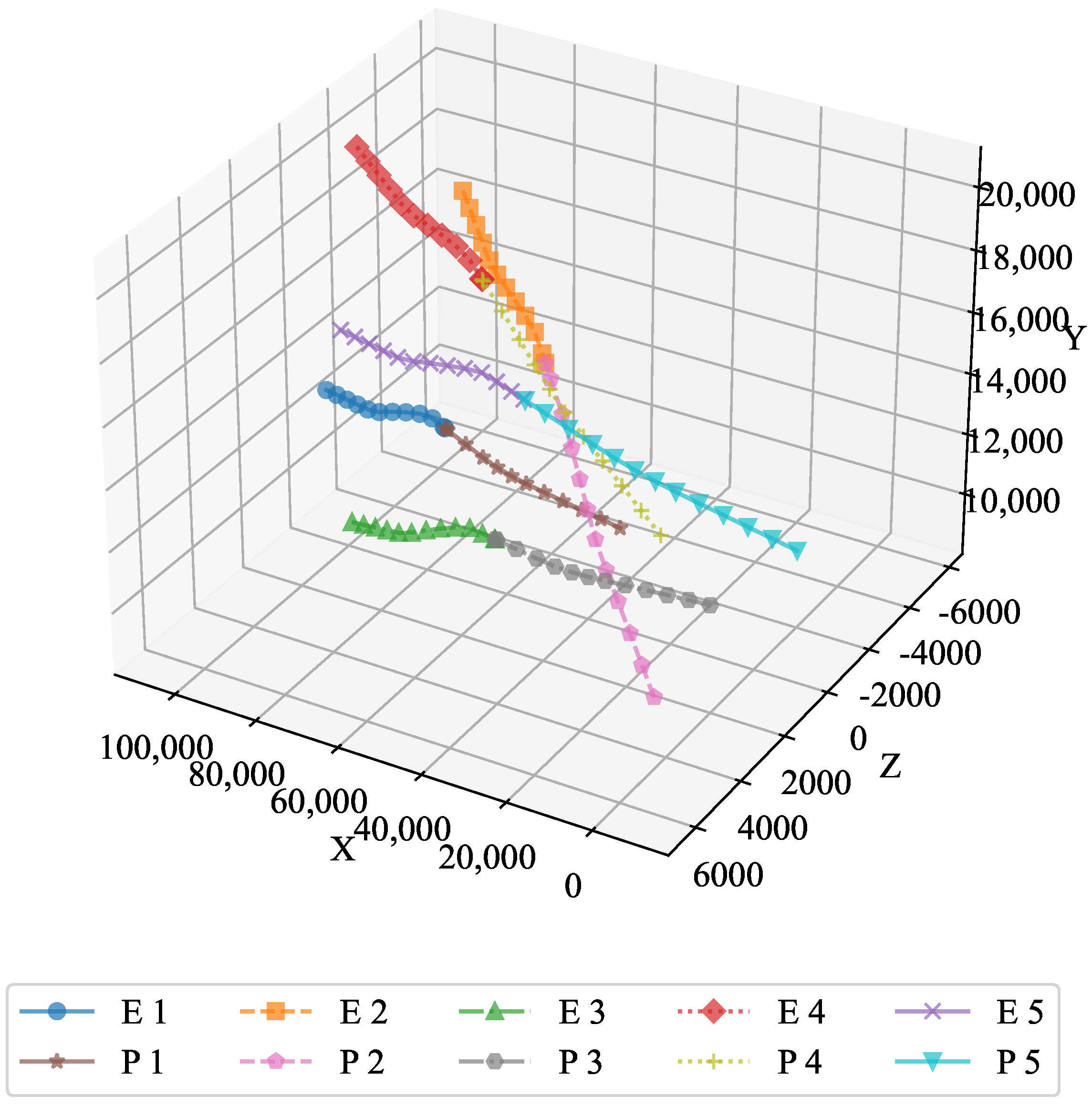
In the first experiment, five pursuers and five evaders each employed the optimal strategy during the simulation. The simulation environment is summarized in Table 2. During the simulation, the Runge–-Kutta method was applied in each iteration.
The optimal trajectory is depicted in Figure 2, which illustrates the efficiency and effectiveness of the optimal feedback strategy. The strategy ensured that both the pursuers and the evaders followed paths that minimized or maximized their respective objectives, demonstrating the capability of the algorithm to handle dynamic environments.
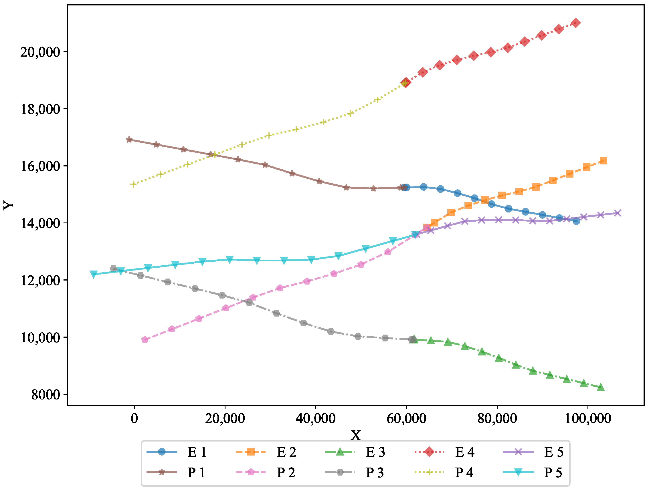
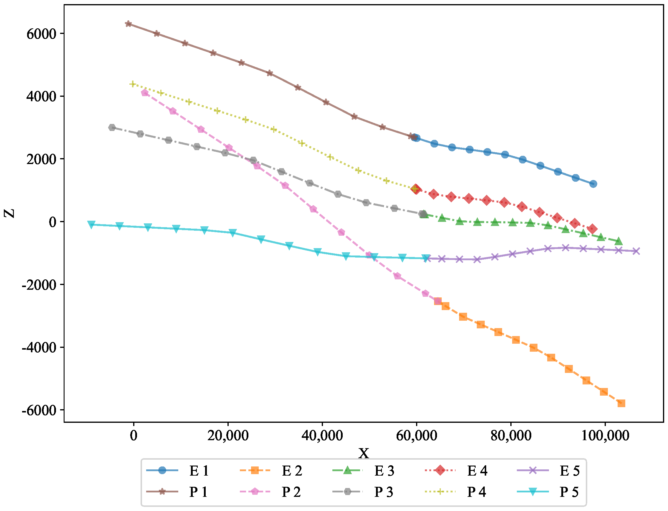
To further analyze the performance, two-dimensional projections in the X–Y and X–Z planes are shown in Figure 3 and Figure 4, respectively. These projections offer a clearer view of the trajectories in different planes, revealing how the optimal state feedback strategy successfully adapted to the spatial constraints. The figures demonstrate the feasibility of the optimal state feedback strategy algorithm proposed in this paper, highlighting its ability to maintain precise control over the motion of the pursuers and evaders, even under varying conditions.
These results show that the strategy not only guided the system toward the desired outcomes, but also did so in a manner that was robust to changes in the initial conditions and perturbations. The efficiency of the strategy is reflected in the smooth and predictable nature of the trajectories, making it an effective solution for real-time applications in pursuit–evasion problems.
The 3D plot illustrates the overall trajectory of the pursuers and evaders. The paths taken by both entities followed smooth, well-defined curves, which highlights the efficacy of the optimal feedback strategy in controlling their movement across three-dimensional space. The optimal feedback strategy is clearly visible, as both the pursuers and the evaders followed well-defined paths. This demonstrates the robustness of the strategy in guiding the system to its desired outcome.
The XY projection highlights the movement of both pursuers and evaders along the horizontal plane. It visually demonstrates how the optimal strategy governed their trajectories, ensuring effective pursuit and evasion on the two-dimensional surface. This projection shows the horizontal movement of the pursuers and evaders, illustrating the optimality of the feedback strategy in maintaining a controlled pursuit−evasion scenario.
In the XZ projection, we can observe the vertical motion of both the pursuers and the evaders. This visualization confirms the optimal feedback strategy’s ability to manage the 3D movement dynamics and maintain the desired behavior in the vertical direction. This view highlights the vertical movement of both the pursuers and evaders, further validating the strategy’s ability to effectively handle 3D motion dynamics.
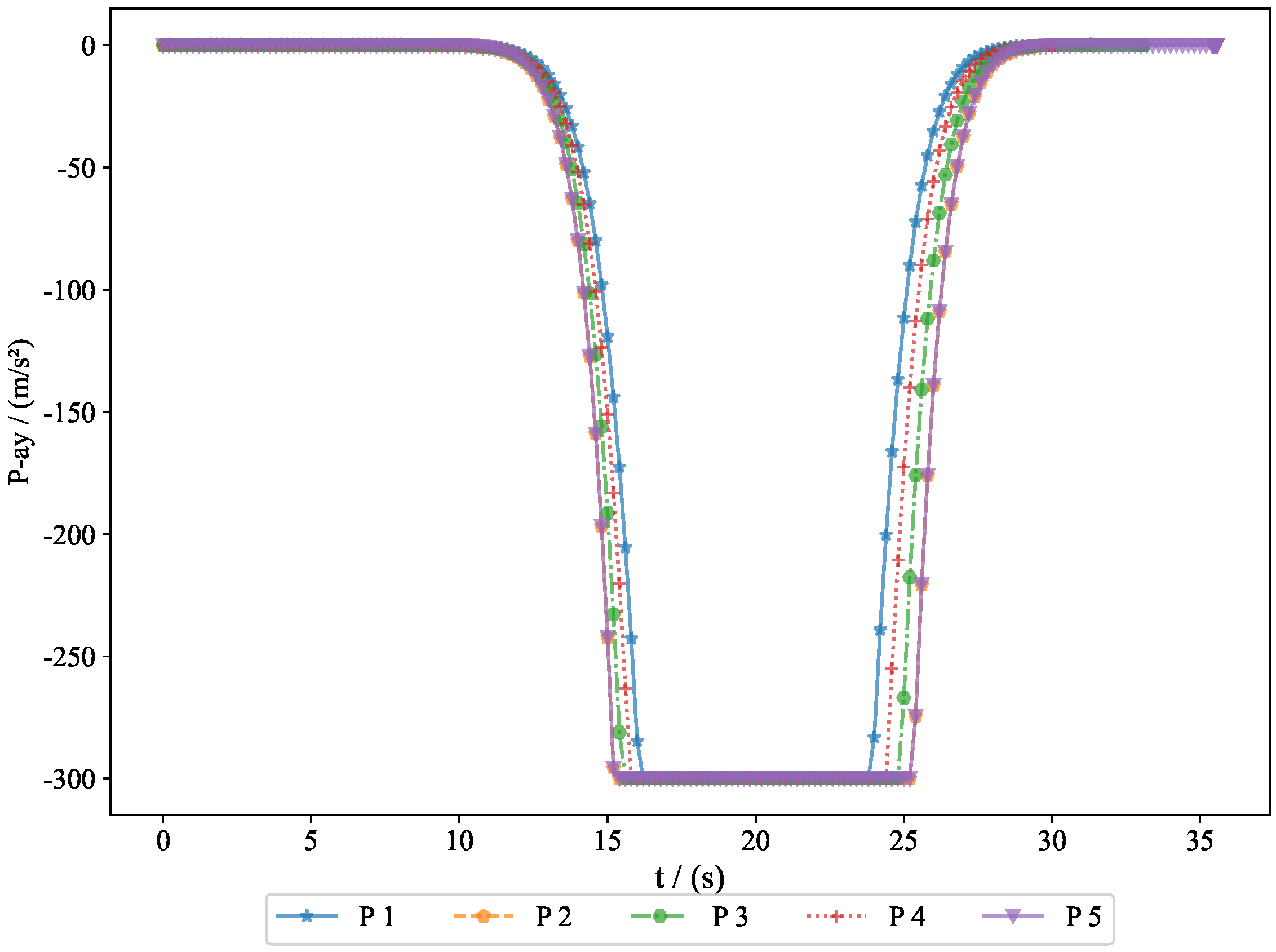
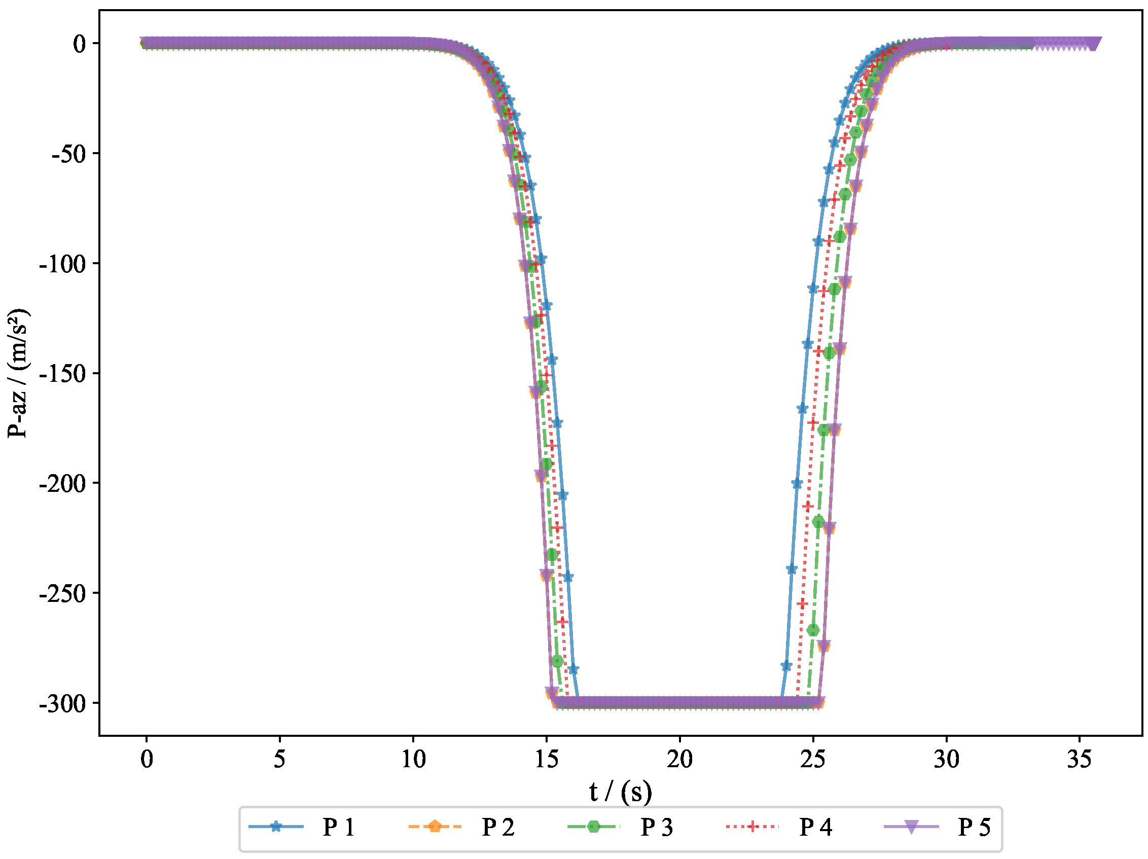
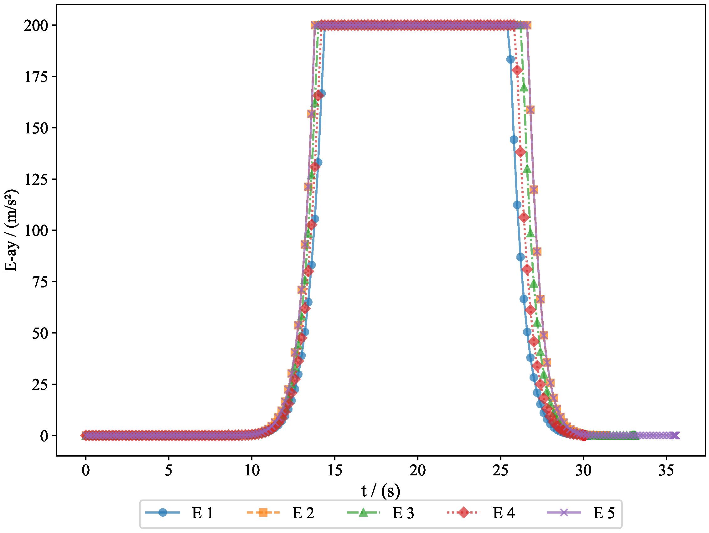
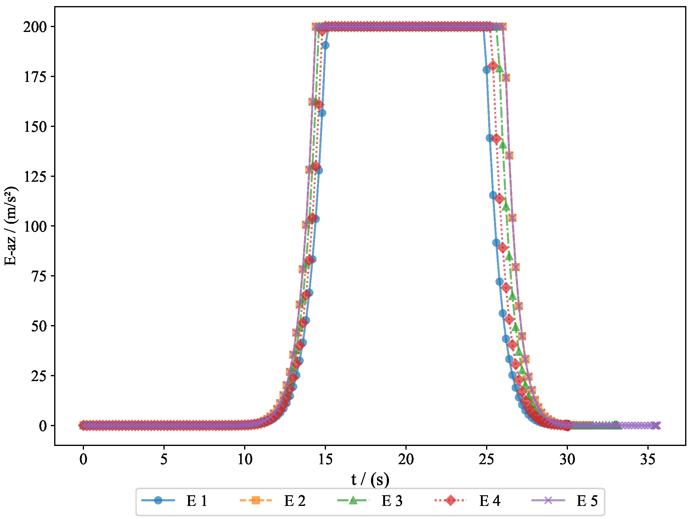
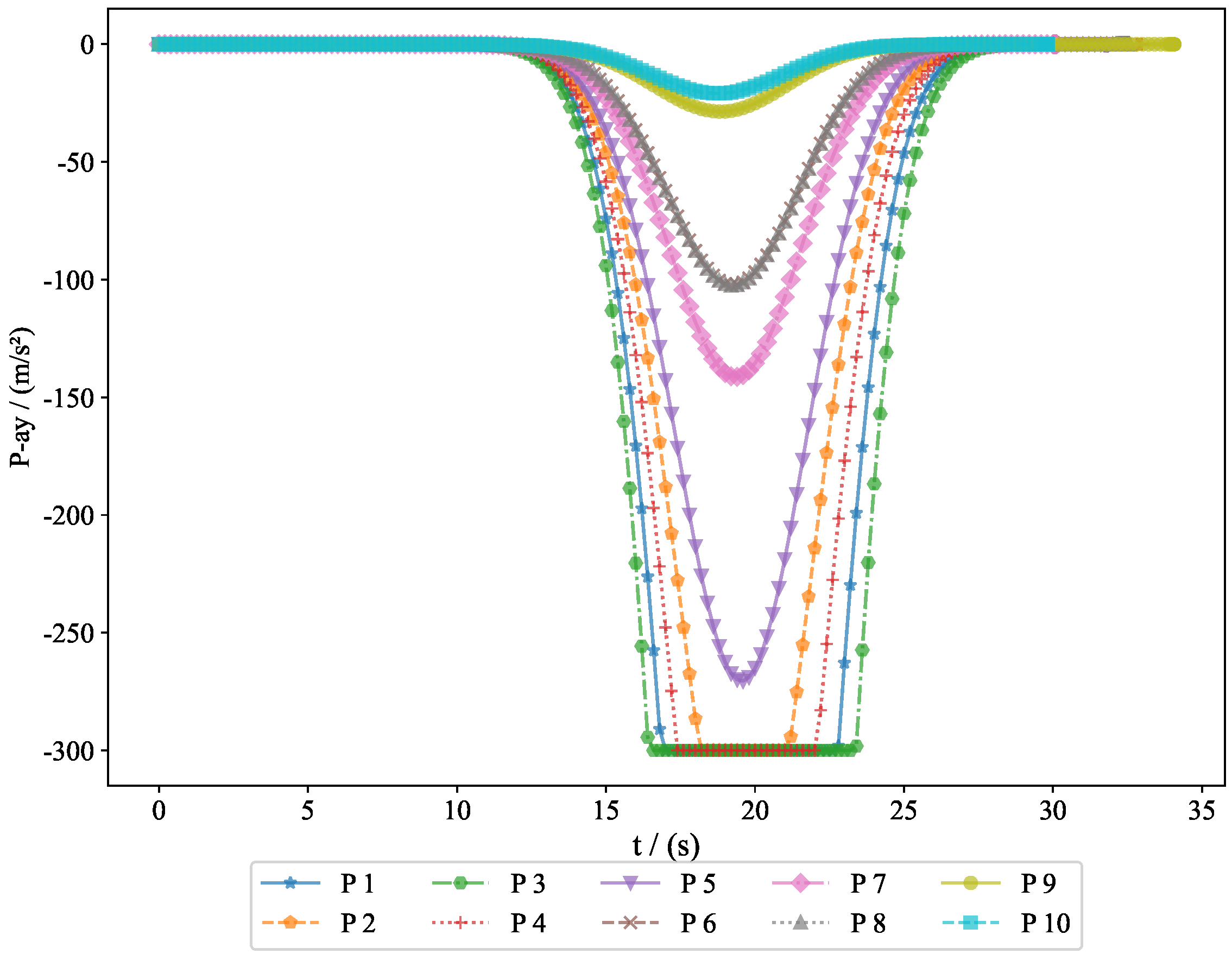
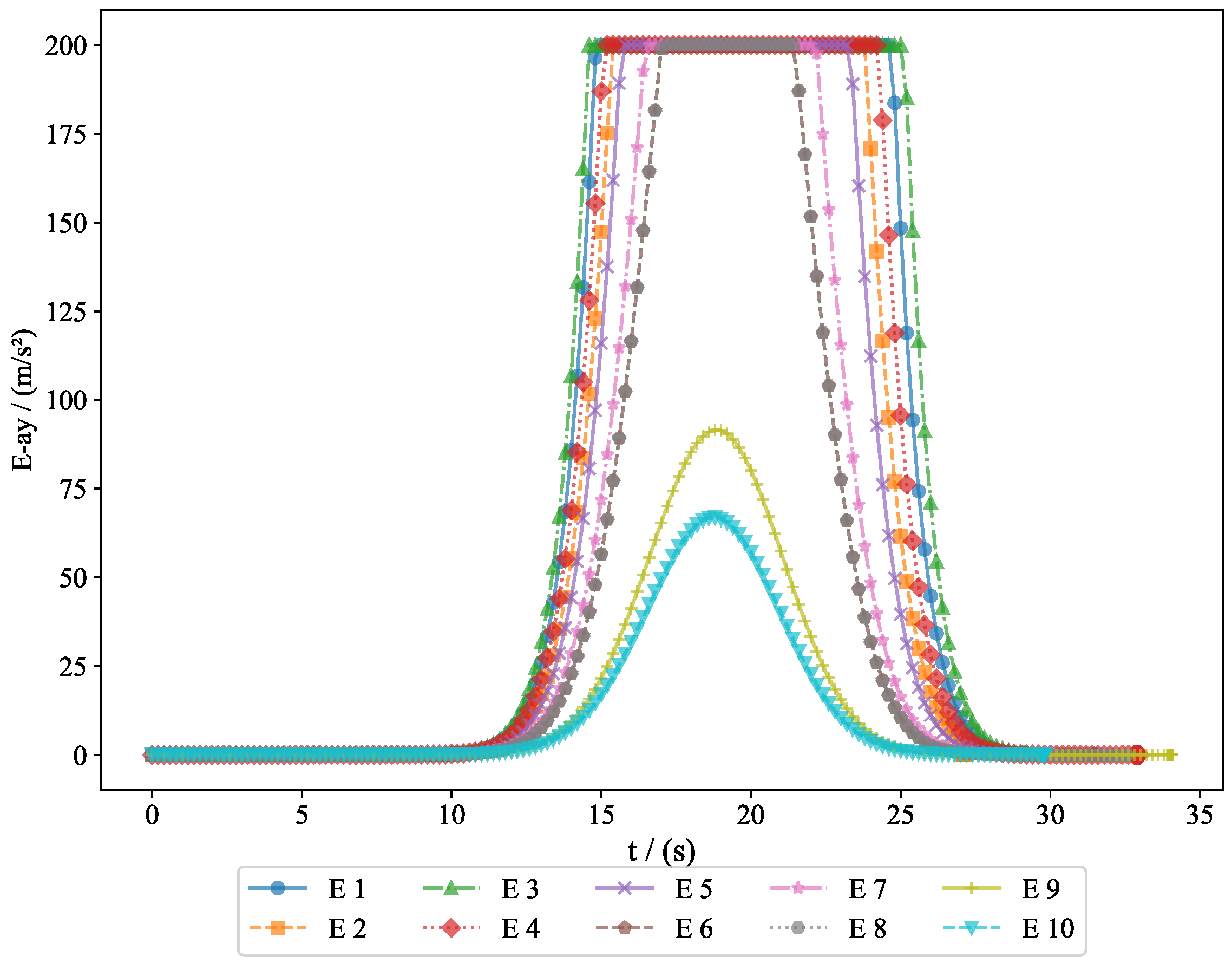
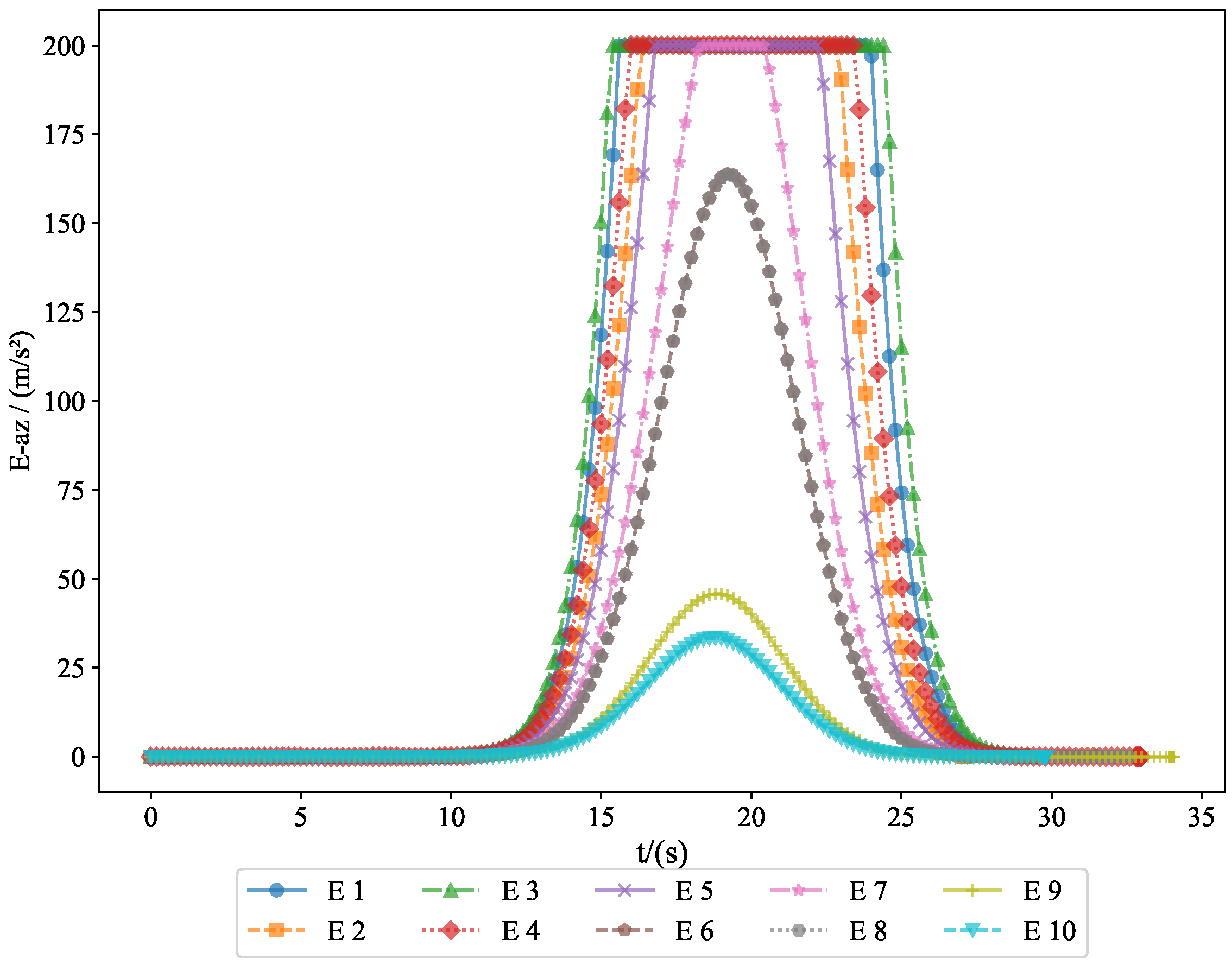
The acceleration variations of the pursuers are shown in Figure 5 and Figure 6, while the acceleration variations of the evaders are shown in Figure 7 and Figure 8. Since the simulation model was based on a missile interception scenario, we introduced a constraint on the normal acceleration to better reflect real-world conditions. The sign of the normal acceleration only indicates direction, with the acceleration starting from zero and eventually returning to zero. This represents the convergence of the line-of-sight angle, achieving a head-on interception. Here, the normal acceleration refers to the acceleration in the velocity frame, where the acceleration directions of the pursuers and evaders are opposite. However, due to the nature of the game theory problem, the optimal strategies of both parties evolve simultaneously.
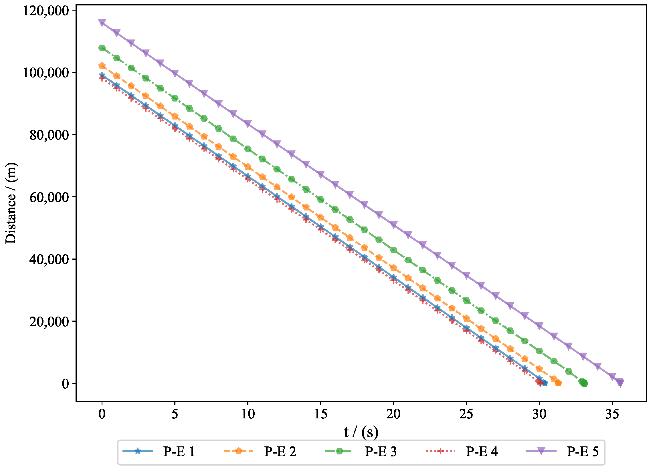
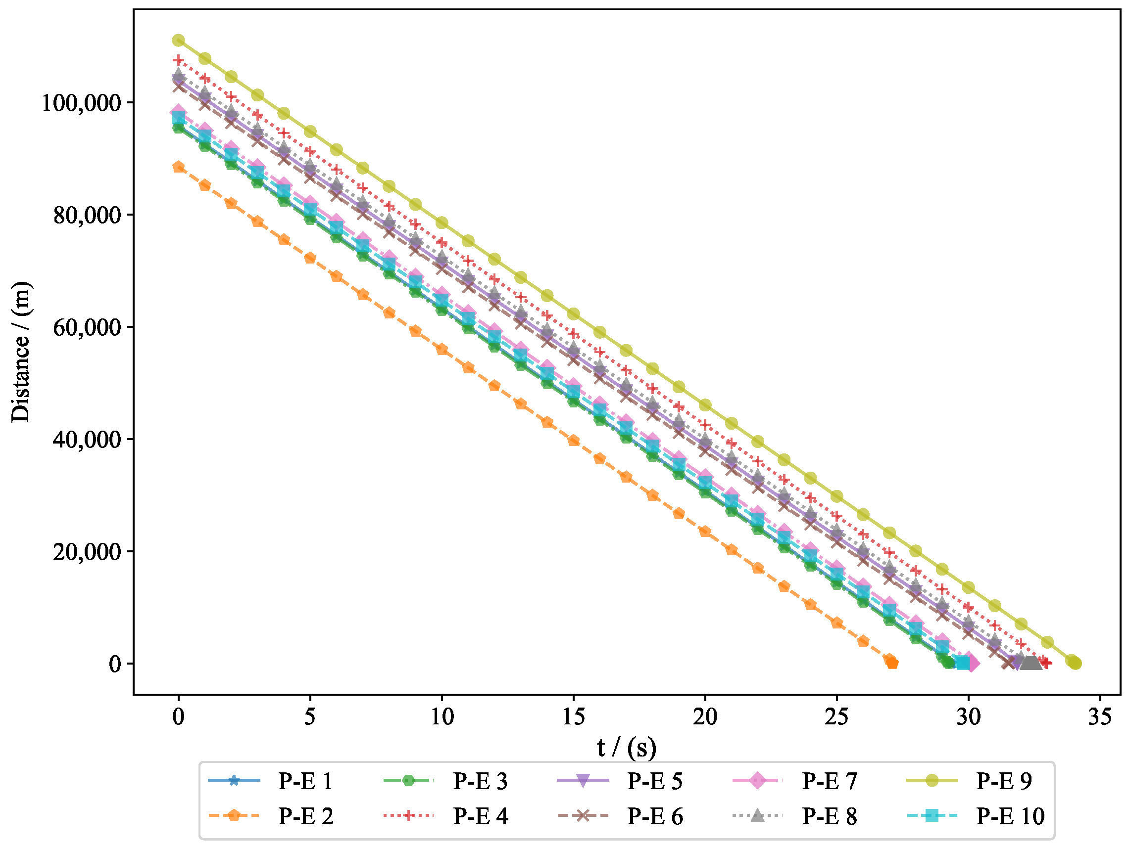
The distance between the evaders and the pursuers is shown in Figure 9, where the final miss distances were 0.53 m , 0.83 m , 0.62 m , 0.94 m , and 0.78 m . In missile interception problems, an interception is typically considered successful when the distance is less than one meter. In this paper, interception is defined by the condition R ˙ > 0 or R < 1 , where R represents the distance between the pursuers and the evaders. The evaders is captured by the pursuers between 30 s and 37 s . Generally, the terminal guidance phase in missile interception lasts between 20 and 40 s, and the results from Experiment 1 fell within this range. The convergence of the final distance and acceleration led to the convergence of the system state. Given that the initial state was bounded and ultimately converged, this demonstrates the bounded nature of the system state. The successful interception of five evaders by the pursuers proves the feasibility of the proposed approach.
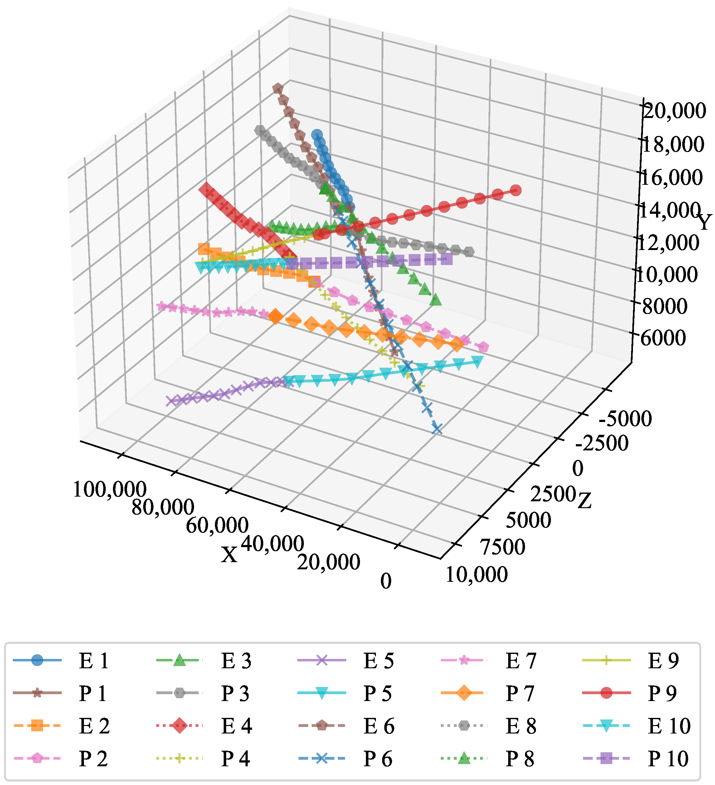
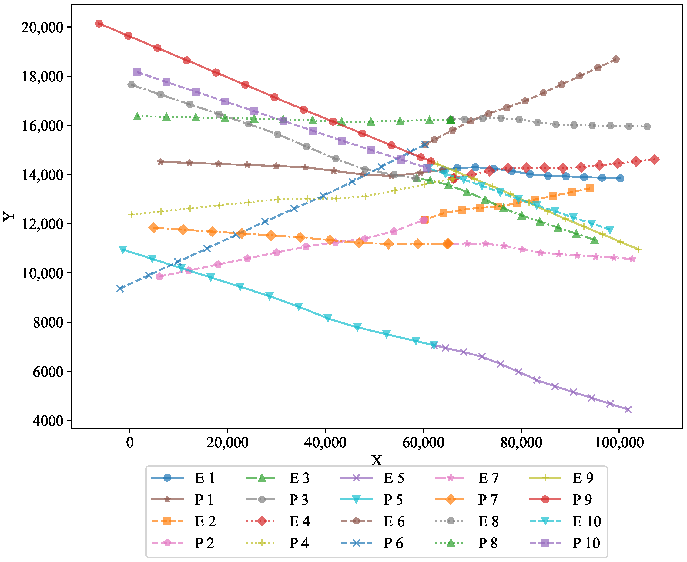
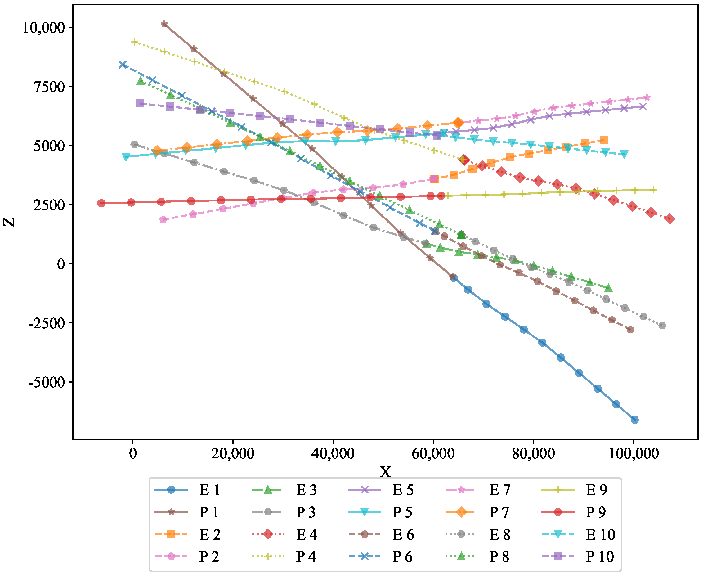
Example 2. 
To verify the feasibility of the algorithm, we increased the number of pursuers and evaders. In Experiment 2, we used 10 pursuers and 10 evaders. Figure 10 shows a 3D interception diagram for the 10VS10 scenario. From this, it can be observed that the double-population game strategy based on MFG is effective in practical situations. This experiment demonstrated the feasibility of the proposed strategy in addressing the evasion problem of nearby populations.
Figure 11 shows the projection in the vertical direction, clearly presenting the positional relationships between the groups. Figure 12 shows the projection in the horizontal direction, further enhancing the understanding of the interactions between the two groups.
To further analyze the movement patterns of the pursuers and evaders, we present the acceleration changes of both the pursuers and evaders along the y-axis and z-axis. Figure 13 shows the acceleration changes of the pursuers along the y-axis, illustrating how the pursuers adjusted their vertical acceleration to respond to the movement of the evaders. Figure 14 displays the acceleration changes of the pursuers along the z-axis, providing further insight into their vertical adjustments.
Similarly, Figure 15 shows the acceleration changes of the evaders along the y-axis, revealing how the evaders modified their vertical acceleration to increase the likelihood of a successful escape. Figure 16 demonstrates the acceleration changes of the evaders along the z-axis, helping us understand how they adjusted their movement strategy to avoid capture by the pursuers. These figures provide important information regarding the acceleration changes of both the pursuers and evaders in three-dimensional space, serving as a basis for subsequent behavioral analysis and strategy optimization.
Figure 17 shows the variation in distance between 10 pursuers and 10 evaders, where the final miss distances were 0.78 m , 0.92 m , 0.94 m , 0.65 m , 0.56 m , 0.79 m , 0.84 m , 0.62 m , 0.98 m , and 0.73 m . As the experiment progressed, the relative positions of the pursuers and evaders continuously changed in three-dimensional space, resulting in fluctuations in the distance between them. By observing this figure, we can clearly see how the pursuers gradually shortened the distance to the evaders, while at certain moments, the evaders successfully increased the distance through effective evasion strategies. These data provided important insights for further analyzing the behavior patterns of chasing and evading, helping to optimize the dynamic interaction strategies between pursuers and evaders.
Based on the many-to-many strategy presented in this article, the experimental results demonstrate that the pursuers successfully captured the evaders, with the system’s state converging to zero and the mean value of the state being finite. At the termination time, the values of the value functions equaled zero. The proposed many-to-one and many-to-many pursuit algorithms effectively enabled the interception of multiple targets.
To test the robustness of the model, we conducted 100 independent experiments with varying initial conditions. The initial positions of the pursuers and evaders were randomly selected, with the constraint that the initial distance between them was always greater than 100,000 m. The initial angles were chosen within a predefined permissible range, to ensure consistency across all trials. The experimental parameters and results are presented in Table 3.
Numerical Stability: To further evaluate the stability of the solution, we varied key system parameters, including control input constraints, system dynamics, and the distribution functions of both the pursuers and evaders, using different distributions—such as exponential, chi-square, Weibull, and normal distributions—for comparison. The results showed that, despite variations in these parameters, the system consistently performed well, with the pursuers successfully intercepting the evaders in most trials. This indicates that the solution to the FBSDEs remained stable and robust, even when small perturbations were introduced into the system parameters.
To provide a more comprehensive view of the advantages and limitations of the MFG approach, we will include a detailed comparison with traditional methods in this paper. Specifically, we compare the performance of the MFG approach and traditional methods in solving the same missile interception problem, particularly in the case of a limited number of targets. Traditional methods typically use proportional guidance laws to intercept targets and assume a smaller number of targets, calculating the behavior of each target individually. In contrast, the MFG approach handles the behavior of large-scale target populations using the mean field assumption. This comparison will help us better demonstrate the advantages of the MFG approach in various scenarios, as well as its potential limitations when the number of targets is limited.
Traditional methods use proportional guidance laws to intercept targets. In comparison, the MFG approach proposed in this paper was tested with 100 targets in 100 experiments, and the results were compared in terms of average miss distance and interception success rate. The experimental results are shown in Table 4.
The primary reason for the failure of traditional methods is that, as the number of targets increases, there is mutual interference between the individuals, making the system dynamics complex and difficult to control. Additionally, the proximity of target groups can significantly affect the interception results, as interactions between targets may lead to misjudgments or deviations in the pursuers’ actions, thereby reducing the success rate of interception. In this case, the density and relative positions of the target group become key factors influencing interception performance.
To overcome these issues, this paper adopts the Mean Field Game (MFG) strategy, which effectively simplifies the behavior model of large-scale target populations using the mean field assumption. Through this approach, we are able to reduce interference between individuals, particularly mitigating the negative impact of groups in proximity on the interception results. The experimental results show that the MFG strategy significantly improved the interception success rate, while reducing the miss distance, demonstrating the effectiveness and advantages of this method in complex environments.

7. Conclusions

This paper used the Mean Field Game approach to deeply explore an optimal control strategy for solving a multi-missile interception problem in three-dimensional space. The study showed that the mean field game model not only effectively overcame the computational explosion problems caused by high dimensions and large-scale systems in traditional methods, but also provided an optimized solution suitable for large-scale, multi-target environments. By introducing the Hamilton–Jacobi–Bellman equation and proving the uniqueness of its solution, this paper provides strong theoretical support for solving complex multi-agent system control problems.
Firstly, this paper derived the motion models of the pursuers and evaders, and described the game behaviors in the multi-missile interception problem through control constraints and cost function design. Using the framework of mean field games, it was shown that the participants could find approximately optimal strategies based on the given population statistics, without being aware of the state of each individual. Furthermore, by leveraging the concept of ϵ -Nash equilibrium, this paper further demonstrated that, within the tolerance range, the participants’ strategies could still minimize costs, ensuring the stability and feasibility of the system.
Finally, the research findings in this paper have broad application prospects, especially in high-risk multi-agent control problems such as missile defense systems. Through the effective application of mean field games, the study not only provides a theoretical basis for the design of practical missile interception systems, but also offers scalable solutions for similar multi-agent systems. The successful application of this theoretical framework demonstrates the immense potential of mean field games in complex multi-target environments. Future research could further explore more efficient solution methods and optimization strategies based on this foundation.

Author Contributions

Conceptualization, Y.B. and D.Z.; methodology, Y.B.; software, Y.B.; validation, Y.B., D.Z. and Z.H.; formal analysis, Y.B.; investigation, D.Z.; resources, Z.H.; data curation, Y.B.; writing—original draft preparation, Y.B.; writing—review and editing, D.Z. and Z.H.; visualization, Y.B.; supervision, D.Z.; project administration, D.Z.; funding acquisition, Z.H. All authors have read and agreed to the published version of the manuscript.

Funding

This research was funded by the National Natural Science Foundation of China, grant number 61773142.

Data Availability Statement

We have added a Data Availability Statement to indicate that no new data were created or analyzed in this study.

Conflicts of Interest

The authors declare no conflicts of interest.

References

  1. Huang, M.; Caines, P.; Malhame, R. Large-population cost-coupled LQG problems: Generalizations to non-uniform individuals. In Proceedings of the 2004 43rd IEEE Conference on Decision and Control (CDC), Nassau, Bahamas, 14–17 December 2004; Volume 4, pp. 3453–3458. [Google Scholar] [CrossRef]
  2. Huang, M.; Caines, P.E.; Malhame, R.P. Large-Population Cost-Coupled LQG Problems With Nonuniform Agents: Individual-Mass Behavior and Decentralized ε-Nash Equilibria. IEEE Trans. Autom. Control. 2007, 52, 1560–1571. [Google Scholar] [CrossRef]
  3. Cecchin, A.; Pra, P.D.; Fischer, M.; Pelino, G. On the Convergence Problem in Mean Field Games: A Two State Model without Uniqueness. SIAM J. Control. Optim. 2019, 57, 2443–2466. [Google Scholar] [CrossRef]
  4. Bensoussan, A.; Frehse, J.; Yam, P. Mean Field Games and Mean Field Type Control Theory; Springer: Berlin/Heidelberg, Germany, 2013. [Google Scholar]
  5. Fathi, M.; Matarasso, A. On the existence of solutions to the Hamilton-Jacobi-Bellman equation for optimal control problems. Appl. Math. Optim. 2007, 56, 229–252. [Google Scholar]
  6. Fleming, W.H.; Soner, H.M. Controlled Markov Processes and Viscosity Solutions; Springer: Berlin/Heidelberg, Germany, 2006. [Google Scholar]
  7. Angel, L.; Sebastian, J.; Saltaren, R.; Aracil, R. RoboTenis System Part II: Dynamics and Control. In Proceedings of the 44th IEEE Conference on Decision and Control, Seville, Spain, 12–15 December 2005; pp. 2030–2034. [Google Scholar] [CrossRef]
  8. Osborne, Y.A.P.; Smears, I. Analysis and Numerical Approximation of Stationary Second-Order Mean Field Game Partial Differential Inclusions. SIAM J. Numer. Anal. 2024, 62, 29. [Google Scholar]
  9. Lasry, J.M.; Lions, P.L. Mean field games. Jpn. J. Math. 2007, 2, 229–257. [Google Scholar] [CrossRef]
  10. Ho, E.; Rajagopalan, A.; Skvortsov, A.; Arulampalam, S.; Piraveenan, M. Game Theory in Defence Applications: A Review. Sensors 2022, 22, 1032. [Google Scholar] [CrossRef]
  11. Cesari, L. Optimization: Theory and Applications; Springer: Berlin/Heidelberg, Germany, 1983. [Google Scholar]
  12. Salonen, H. On the existence of Nash equilibria in large games. Int. J. Game Theory 2010, 39, 351–357. [Google Scholar]
  13. Dayanikli, G.; Laurière, M. Multi-population Mean Field Games with Multiple Major Players: Application to Carbon Emission Regulations. In Proceedings of the 2024 American Control Conference (ACC), Toronto, ON, Canada, 8–9 July 2024; pp. 5075–5081. [Google Scholar] [CrossRef]
  14. Nash, J.F. Equilibrium points in n-person games. Proc. Natl. Acad. Sci. USA 1950, 36, 48–49. [Google Scholar] [CrossRef]
  15. Turetsky, V.; Shinar, J. Missile guidance laws based on pursuit–evasion game formulations. Automatica 2003, 39, 607–618. [Google Scholar] [CrossRef]
  16. Sun, Z.; Yang, J. Multi-missile interception for multi-targets: Dynamic situation assessment, target allocation and cooperative interception in groups. J. Frankl. Inst. 2022, 359, 7745–7770. [Google Scholar] [CrossRef]
  17. Carmona, R.; Delarue, F. Probability Theory and Stochastic Modelling: Probabilistic Theory of Mean Field Games with Applications I; Springer International Publishing: Berlin/Heidelberg, Germany, 2018. [Google Scholar]
  18. Toumi, N.; Malhamé, R.; Ny, J.L. A mean field game approach for a class of linear quadratic discrete choice problems with congestion avoidance. Automatica 2024, 160, 13. [Google Scholar] [CrossRef]
  19. Song, S.H.; Ha, I.J. A Lyapunov-like approach to performance analysis of 3-dimensional pure PNG laws. IEEE Trans. Aerosp. Electron. Syst. 1994, 30, 238–248. [Google Scholar] [CrossRef]
  20. Cannarsa, P.; Capuani, R.; Cardaliaguet, P. Mean field games with state constraints: From mild to pointwise solutions of the PDE system. Calc. Var. Partial. Differ. Equations 2021, 60, 108. [Google Scholar] [CrossRef]
  21. Song, J.; Zhang, X.; Wang, L. Impact Angle Constrained Guidance against Non-maneuvering Targets. AIAA J. Guid. Control. Dyn. 2023, 46, 1556–1565. [Google Scholar] [CrossRef]
  22. Li, B.; Zhang, W.; Sun, Z. Guidance for Intercepting High-Speed Maneuvering Targets. J. Guid. Control. Dyn. 2021, 44, 2282–2293. [Google Scholar]
  23. Hou, M.; Liang, X.; Duan, G. Adaptive block dynamic surface control for integrated missile guidance and autopilot. Chin. J. Aeronaut. 2013, 26, 741–750. [Google Scholar] [CrossRef]
  24. Oza, H.B.; Padhi, R. Impact-Angle-Constrained Suboptimal Model Predictive Static Programming Guidance of Air-to-Ground Missiles. J. Guid. Control Dyn. 2012, 35, 153–164. [Google Scholar] [CrossRef]
  25. Souganidis, P.E.; Zariphopoulou, T. Mean field games with unbounded controlled common noise in portfolio management with relative performance criteria. Math. Financ. Econ. 2024, 18, 28. [Google Scholar]
  26. Ran, M.; Wang, Q.; Hou, D.; Dong, C. Backstepping design of missile guidance and control based on adaptive fuzzy sliding mode control. Chin. J. Aeronaut. 2014, 27, 634–642. [Google Scholar] [CrossRef]
  27. Firoozi, D.; Jaimungal, S.; Caines, P.E. Convex analysis for LQG systems with applications to major–minor LQG mean-field game systems. Syst. Control. Lett. 2020, 142, 104725. [Google Scholar] [CrossRef]
  28. Huang, M. Linear-quadratic mean field games with a major player: Nash certainty equivalence versus master equations. Commun. Inf. Syst. 2021, 21, 213–242. [Google Scholar] [CrossRef]
  29. Firoozi, D.; Jaimungal, S.; Caines, P.E. Exploratory LQG mean field games with entropy regularization. J. Optim. Theory Appl. 2020, 184, 211–237. [Google Scholar] [CrossRef]
  30. Engwerds, J.C.; van den Broek, W.A.; Schumacher, J.M. Feedback Nash equilibria in uncertain infinite time horizon differential games. In Proceedings of the 14th International Symposium of Mathematical Theory of Networks and Systems, Perpignan, France, 19–23 June 2000; pp. 1–6. [Google Scholar]
  31. Carlini, E.; Silva, F.J.; Zorkot, A. A Lagrange-Galerkin scheme for first order mean field games systems. arXiv 2023, arXiv:2303.14941. [Google Scholar] [CrossRef]
  32. Hintermüller, M.; Surowiec, T.M.; Theiß, M. On a Differential Generalized Nash Equilibrium Problem with Mean Field Interaction. SIAM J. Optim. 2024, 33, 1587–1620. [Google Scholar] [CrossRef]
  33. Li, M.; Li, N.; Wu, Z. Linear–quadratic mean-field game for stochastic systems with partial observation. Automatica 2025, 171, 111821. [Google Scholar] [CrossRef]
  34. Hu, Y.; Peng, S. Solution of forward-backward stochastic differential equations. Probab. Theory Relat. Fields 1995, 103, 273–283. [Google Scholar] [CrossRef]
  35. Bensoussan, A.; Cass, T.; Chau, M.H.M.; Yam, S.C.P. Mean Field Games with Parametrized Followers. IEEE Trans. Autom. Control. 2019, 65, 12–27. [Google Scholar]
Figure 1. Model of movement in 3D space.
Aerospace 12 00302 g001
Figure 2. Three−dimensional trajectory of pursuers and evaders.
Aerospace 12 00302 g002
Figure 3. XY projection of the trajectories.
Aerospace 12 00302 g003
Figure 4. XZ projection of the trajectories.
Aerospace 12 00302 g004
Figure 5. Pursuer’s acceleration along the y−axis.
Aerospace 12 00302 g005
Figure 6. Pursuer’s acceleration along the z−axis.
Aerospace 12 00302 g006
Figure 7. Evader’s acceleration along the y−axis.
Aerospace 12 00302 g007
Figure 8. Evader’s acceleration along the z−axis.
Aerospace 12 00302 g008
Figure 9. Variation in the distance.
Aerospace 12 00302 g009
Figure 10. Three−dimensional interception diagram for 10VS10.
Aerospace 12 00302 g010
Figure 11. XY projection in the vertical direction.
Aerospace 12 00302 g011
Figure 12. XZ projection in the horizontal direction.
Aerospace 12 00302 g012
Figure 13. Pursuer’s y−axis acceleration.
Aerospace 12 00302 g013
Figure 14. Pursuer’s z−axis acceleration.
Aerospace 12 00302 g014
Figure 15. Evader’s y−axis acceleration.
Aerospace 12 00302 g015
Figure 16. Evader’s z−axis acceleration.
Aerospace 12 00302 g016
Figure 17. Distance variation between 10 pursuers and 10 evaders.
Aerospace 12 00302 g017
Table 1. Table of symbols and coordinate systems.
SymbolDescriptionCoordinate System
( X I , Y I , Z I ) Inertial reference coordinate systemInertial
( X L , Y L , Z L ) Line-of-sight (LOS) coordinate systemLOS
( X E , Y E , Z E ) Velocity coordinate system of the i-th pursuerPursuer
v E i Velocity of the i-th evaderEvader
v P i Velocity of the i-th pursuerPursuer
A P i Acceleration of the i-th pursuerPursuer
A E i Acceleration of the i-th evaderEvader
γ P i Angle between the acceleration of the i-th pursuer and axis Y P i Pursuer
γ E i Angle between the acceleration of the i-th evader and axis Y E Evader
R P i Distance between the i-th pursuer and the evaderSpatial
θ L i , φ L i LOS angles between the evader and the i-th pursuer relative to the inertial reference coordinate systemLOS
θ P i , φ P i Elevation and azimuth angles of v P i relative to the LOS coordinate system from pointing toward EPursuer
θ E i , φ E i Elevation and azimuth angles of v E i relative to the LOS coordinate system from E i pointing toward P i Evader
A z P i , A y P i Projections of the pursuer’s normal acceleration on the Z P i and Y P i axes in the velocity coordinate systemPursuer
A z E i , A y E i Projections of the evader’s normal acceleration on the Z E i and Y E i axes in the velocity coordinate systemEvader
Table 2. Experiment environment.
ItemEnvironment
Development languagePython
LibraryNumpy
Disk capacity2 T
RAM32 G
CPUi7 2.2 GHZ
OSUbuntu 16.04
Table 3. Experimental setup and parameters.
ParameterValue
Initial distance100,000
Initial number of evaders50
Initial number of pursuers50
Evader initial elevation angle [ 20 , 20 ] (elevation), [ 160 , 200 ] (azimuth)
pursuer initial azimuth angle [ 20 , 20 ] (elevation), [ 20 , 20 ] (azimuth)
Iteration time0.1 s–0.5 s
Maximum normal acceleration20–40 g
Number of experiments100 experiments
Exponential distribution98 successful, 2 failed
Chi-square distribution95 successful, 5 failed
Weibull distribution97 successful, 3 failed
Normal distribution99 successful, 1 failed
Table 4. Experimental setup and results.
MetricProportional Guidance LawMean Field Game
Initial Number of Evaders100100
Initial Number of Pursuers100100
Number of Experiments100100
Miss Distance0.93 m0.82 m
Interception Success Rate86 successful97 successful
Disclaimer/Publisher’s Note: The statements, opinions and data contained in all publications are solely those of the individual author(s) and contributor(s) and not of MDPI and/or the editor(s). MDPI and/or the editor(s) disclaim responsibility for any injury to people or property resulting from any ideas, methods, instructions or products referred to in the content.

