
A Patrol Route Design for Inclined Geosynchronous Orbit Satellites in Space Traffic Management


Abstract
1. Introduction
2. Materials and Methods
2.1. Calculate the Crossing Position and Time of the IGSO Targets
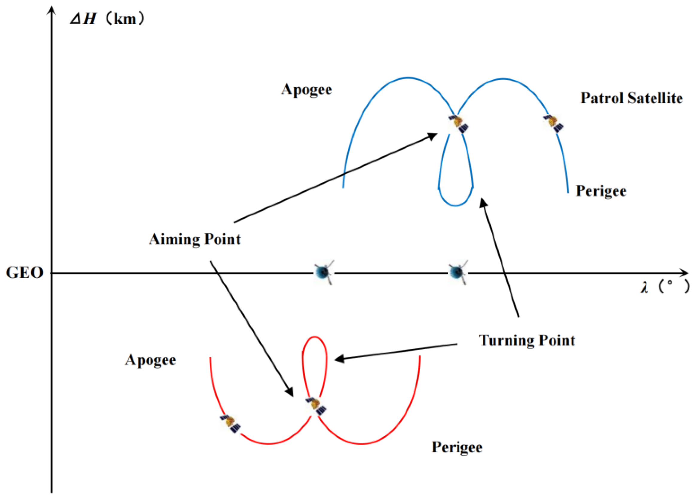
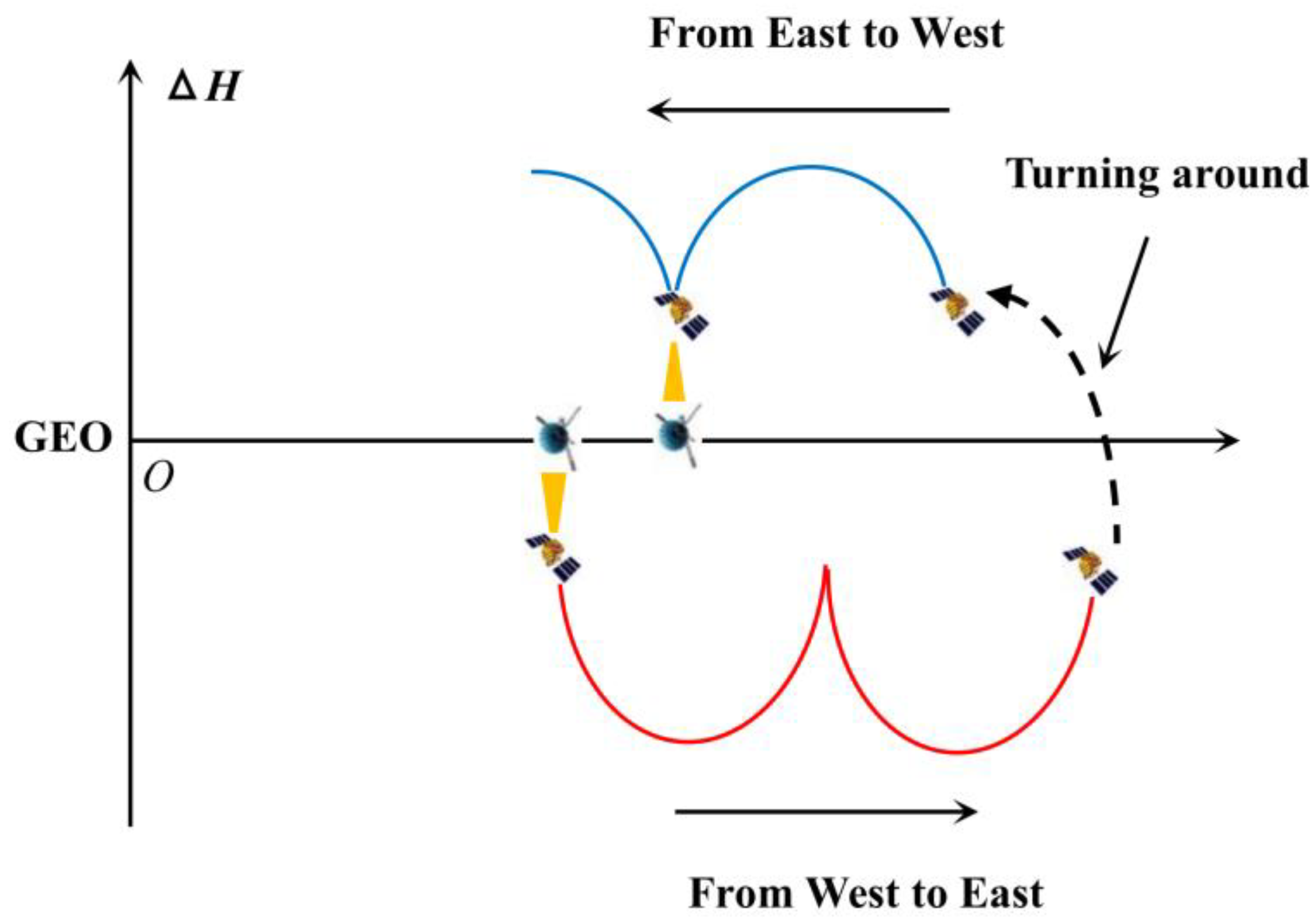
2.2. Design a Spiral Trajectory That Satisfies the Desired Patrol Time
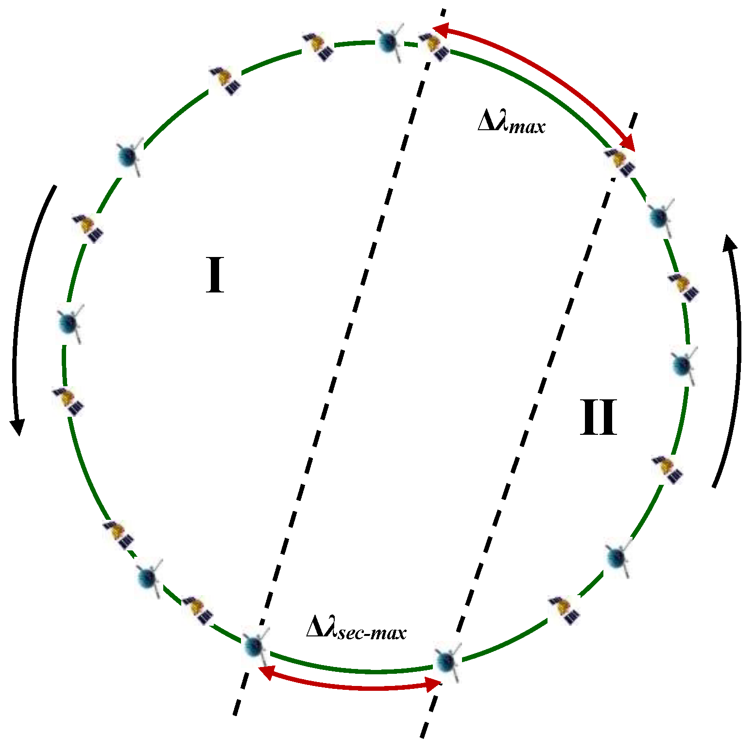
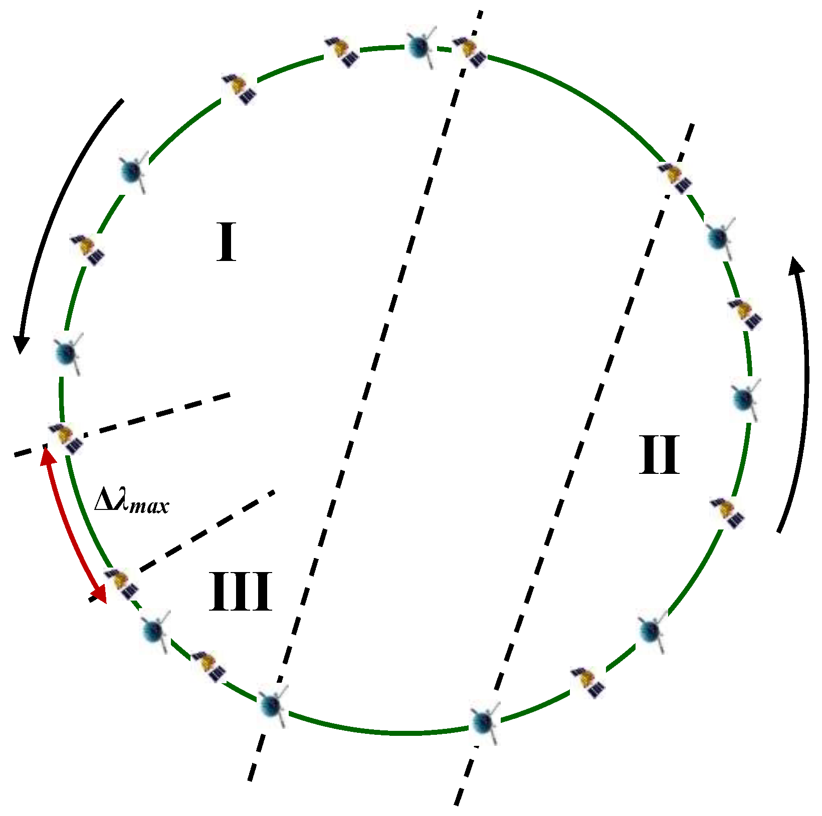
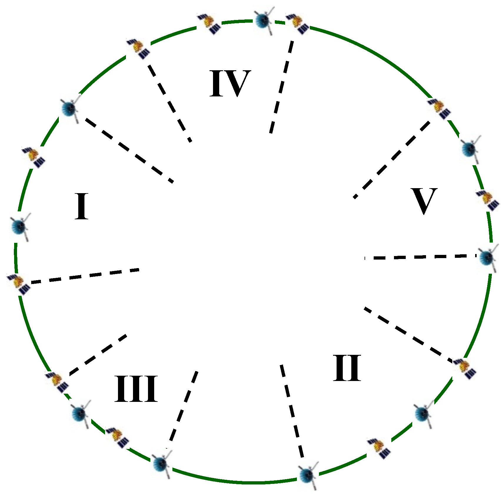
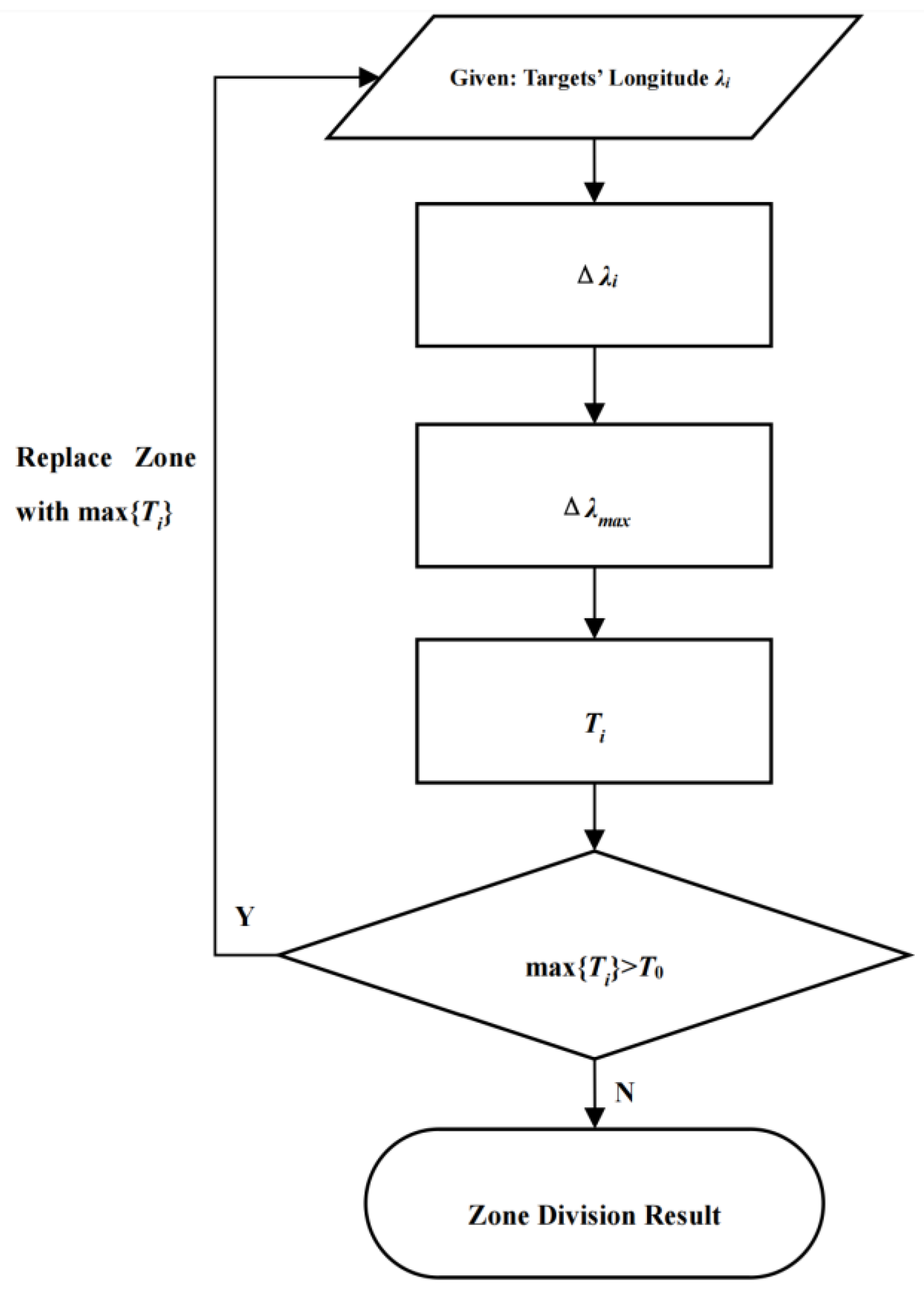
2.3. Divide IGSO Targets into Regions Using the Dichotomy Approach
2.4. Calculate the Bidirectional Longitude Drift Rate Within Each Region
2.5. Determine the Starting Position of Patrol for Each Region
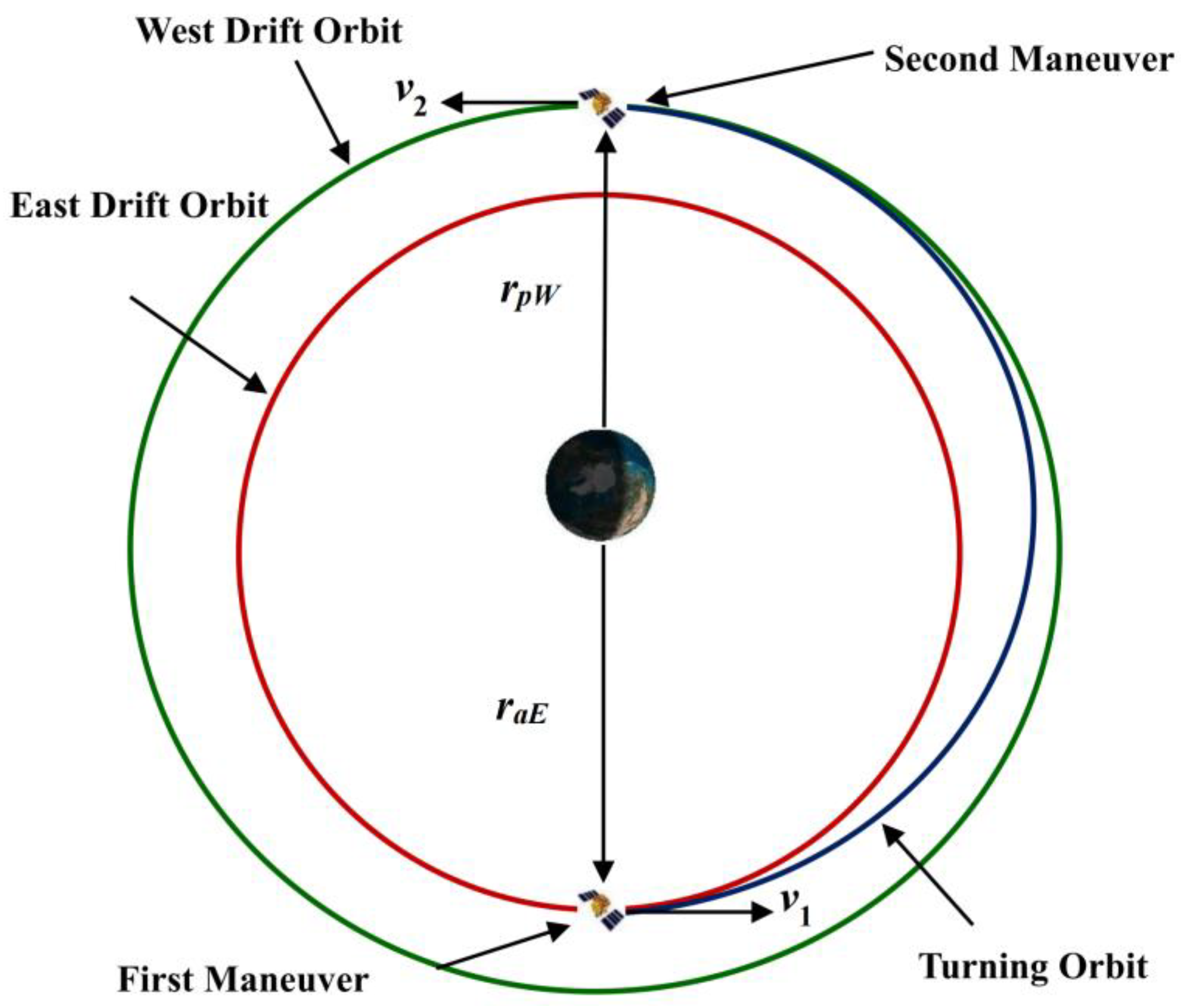
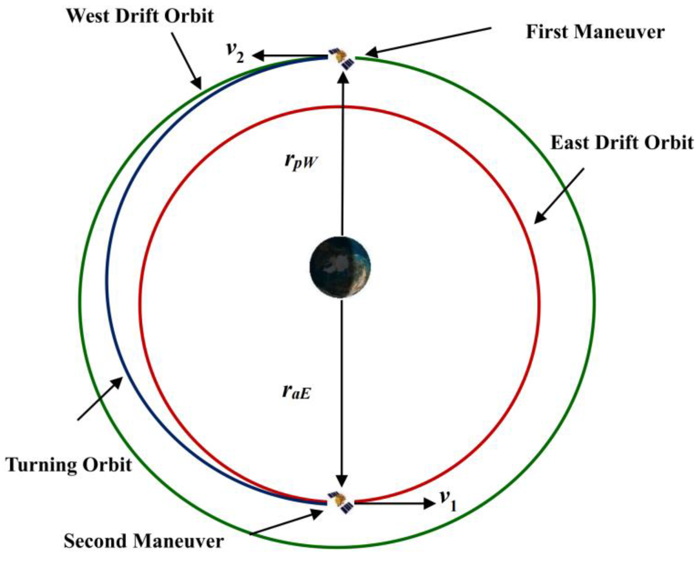
2.6. Determine the Transfer Orbit for Each Region
3. Results
3.1. Calculate the Crossing Position and Crossing Time of the IGSO Targets
3.2. Design a Spiral Trajectory That Satisfies Desired Patrol Time
3.3. Divide IGSO Targets into Regions Based on Dichotomy Approach
3.4. Calculate the Bidirectional Longitude Drift Rate Within Each Region
3.5. Determine the Starting Position of the Patrol for Each Region
3.6. Determine the Transfer Orbit for Each Region
4. Case Study
5. Conclusions
6. Patents
Author Contributions
Funding
Data Availability Statement
Conflicts of Interest
Appendix A

| D | Longitude drift rate |
| Patrol satellite orbital element | |
| ac | Semi-major axis of GEO |
| Target orbital element | |
| Time of the crossing point | |
| Geocentric distance of the crossing point | |
| Ascending intersection angle of the crossing point | |
| ucross | Argument of latitude of the crossing point |
| μ | The gravitational constant of the Earth |
| E | Eccentric anomaly |
| Tt | Target’s orbital period |
| Te | The period of rotation of the Earth |
| Ωcross | Right ascension of the ascending node of the crossing point |
| vturn | Velocity of the turning point |
| rturn | Position of the turning point |
| vaim | Velocity of the aiming point |
| raim | Position of the aiming point |
| Tring | The period of the spiral ring |
| νturn | Energy parameter at the turning point |
| Tins | Time of the earliest aiming point |
| λi (i = 1, 2, …, n) | Targets’ sub-satellite point longitude |
| Δλi (i = 1, 2, …, n) | Difference in longitude between adjacent targets |
| Δλmax | Largest longitude difference gap between targets |
| Δλsec-max | Second largest longitude difference gap between targets |
| Dmin | Min longitude drift rate |
| Dmax | Max longitude drift rate |
| Ti (i = I, II, …) | Periods of the zones |
| T0 | The given limitation period |
| Zi (i = 1, 2, …, N) | Target set in zone i |
| Mi (i = 1, 2, …, N) | Number of targets in zone i |
| DE | Eastward longitude drift rate of the patrol satellite |
| DW | Westward longitude drift rate of the patrol satellite |
| QE | Targets with the same remainder of DE |
| QW | Targets with the same remainder of DW |
| Δq | Region thresholds for the target set |
| TE | Initial time of the eastward drift |
| TW | Initial time of the westward drift |
| λE | Initial position of the eastward drift |
| λW | Initial position of the westward drift |
| aE | Semi-major axis of the eastward drift orbit |
| aW | Semi-major axis of the westward drift orbit |
| aT | Semi-major axis of the transfer orbit |
| raE | Position of the eastward drift orbit apogee |
| rpE | Position of the eastward drift orbit perigee |
| raW | Position of the westward drift orbit apogee |
| rpW | Position of the westward drift orbit perigee |
| vaE | Velocity of the eastward drift orbit apogee |
| vpE | Velocity of the eastward drift orbit perigee |
| vaW | Velocity of the westward drift orbit apogee |
| vpW | Velocity of the westward drift orbit perigee |
| v1 | Velocity of the first maneuver |
| v2 | Velocity of the second maneuver |
| rp | Position of the patrol orbit perigee |
| ra | Position of the patrol orbit apogee |
| vp | Velocity of the patrol orbit perigee |
| va | Velocity of the patrol orbit apogee |
References
- Quan, H.; Li, X. Preliminary Research on Space Traffic Management Standards System. Space Debris Res. 2021, 21, 50–57. [Google Scholar]
- Duan, F. Research on the Shift from Space Traffic Management to Space Traffic Coordination in the United States. Space Debris Res. 2022, 22, 66–71. [Google Scholar]
- Yao, W.; Feng, S.; Chen, L. Study on the Development of Space Traffic Management. Aerosp. China 2021, 3, 49–52. [Google Scholar]
- Feng, S.; Yao, W.; Chen, L. Discussion on the Framework of Space Traffic Management System. Aerosp. China 2021, 9, 38–43. [Google Scholar]
- Space Debris Mitigation Guidelines; Revision 2; IADC: Houston, TX, USA, 2020.
- ESA’s Annual Space Environment Report; ESA: Paris, France, 2024.
- Available online: https://www.ucsusa.org/resources/satellite-database (accessed on 1 May 2023).
- Shen, H.; Tsiotras, P. Optimal Scheduling for Servicing Multiple Satellites in a Circular Constellation. In Proceedings of the AIAA/AAS Astrodynamics Specialist Conference and Exhibit, Monterey, CA, USA, 5–8 August 2002. [Google Scholar]
- Alfriend, K.T.; Creamer, N.G.; Lee, D.J. Optimal Servicing of Geosynchronous Satellites. J. Guid. Control Dyn. 2006, 29, 203–206. [Google Scholar]
- Zhou, Y.; Yan, Y.; Huang, X.; Kong, L. Mission planning optimization for multiple geosynchronous satellites refueling. Adv. Space Res. 2015, 56, 2612–2625. [Google Scholar]
- Zhang, Y.; Xu, Y.; Zhou, H. Theory and Design Method of Special Space Orbit; National Defense Industry Press: Beijing, China, 2015. [Google Scholar]
- Zheng, L.; Xu, Y.; Zhu, D. Cruise orbit design for multiple geostationary orbit targets. Aerosp. Control Appl. 2016, 42, 37–41. [Google Scholar]
- Bo, X.; Feng, Q. Research on constellation refueling based on formation flying. Acta Astronaut. 1987, 68, 1987–1995. [Google Scholar]
- Madakat, D.; Morio, J.; Vanderpooten, D. Biobjective planning of an active debris removal mission. Acta Astronaut. 2013, 84, 182–188. [Google Scholar]
- Du, B.; Zhao, Y.; Dutta, A.; Yu, J.; Chen, X. Optimal scheduling of multispacecraft refueling based on cooperative maneuver. Adv. Space Res. 2015, 55, 2808–2819. [Google Scholar] [CrossRef]
- Jackson, B. Minimum energy maneuvering strategies for multiple satellite inspection missions. In Proceedings of the IEEE Aerospace Conference, Big Sky, MT, USA, 5–12 March 2005. [Google Scholar]
- Zhang, J.; Parks, G.T.; Luo, Y.Z. Multisatellite Refueling Optimization Considering the J2 Perturbation and Window Constraints. J. Guid. Control Dyn. 2014, 37, 111–122. [Google Scholar]
- Zhou, Y.; Yan, Y.; Huang, X.; Kong, L. Optimal scheduling of multiple geosynchronous satellites refueling based on a hybrid particle swarm optimizer. Aerosp. Sci. Technol. 2015, 47, 125–134. [Google Scholar]
- Zhang, T.J.; Yang, Y.K.; Wang, B.H.; Li, Z.; Shen, H.X.; Li, H.N. Optimal scheduling for location geosynchronous satellites refueling problem. Acta Astronaut. 2019, 163, 264–271. [Google Scholar]
- Xiao, D.; Xu, B.; Gao, Y. Optimization of Supply Orbit for Heterogeneous Constellations Based on Companion Flight Mode Chinese Science. Phys. Mech. Astron. 2012, 12, 67–77. [Google Scholar]
- Xiao, D.; Zhu, Q.; Zu, L. Research on Multi Supply Tasks of Heterogeneous Constellations Based on Accompanying Flight Mode. Shanghai Aerosp. 2016, 33, 9–14. [Google Scholar]
- Yu, J.; Yu, Y.-G.; Hao, D.; Chen, X.-Q.; Liu, H.-Y. Biobjective mission planning for geosynchronous satellites on-orbit refueling. Proc. Inst. Mech. Eng. 2019, 233, 686–697. [Google Scholar]
- Prodhon, C.; Prins, C. A survey of recent research on location-routing problems. Eur. J. Oper. Res. 2014, 238, 1–17. [Google Scholar]
- Shen, H.; Tsiotras, P. Peer-to-Peer Refueling for Circular Satellite Constellations. J. Guid. Control Dyn. 2005, 28, 1220–1230. [Google Scholar]
- Salazar, A.; Tsiotras, P. An auction algorithm for allocating fuel in satellite constellations using peer-to-peer refueling. In Proceedings of the 2006 American Control Conference, Minneapolis, MN, USA, 14–16 June 2006. [Google Scholar]
- Rui, B.L.; Ferreira, C.; Santos, B.S. A simple and effective evolutionary algorithm for the capacitated location routing problem. Comput. Oper. Res. 2016, 70, 155–162. [Google Scholar]
- Tang, R.; Wang, W.; Fu, X. Orbit selection and optimization for approaching multiple Walker constellation satellites. Comput. Simul. 2008, 4, 59–62. [Google Scholar]
- Dutta, A.; Tsiotras, P. Greedy Random Adaptive Search Procedure for Optimal Scheduling of P2P Satellite Refueling. In Proceedings of the AAS/AIAA Space Flight Mechanics Meeting, American Astronautical Society Paper 07-150, Sedona, Arizona, 28 January–1 February 2007. [Google Scholar]
- Dutta, A.; Tsiotras, P. Network Flow Formulation for an Egalitarian P2P Refueling Strategy. In Proceedings of the AAS/AIAA Space Flight Mechanics Meeting, American Astronautical Society Paper 07-151, Sedona, Arizona, 28 January–1 February 2007. [Google Scholar]
- Dutta, A.; Tsiotras, P. Asynchronous optimal mixed P2P satellite refueling strategies. Astronaut. Sci. 2006, 54, 543–565. [Google Scholar]
- Dutta, A.; Tsiotras, P. An Egalitarian Peer-to-Peer Satellite Refueling Strategy. J. Satell. Rocket. 2008, 45, 608–618. [Google Scholar]
- Chen, X.Q.; Yu, J. Optimal mission planning of GEO on-orbit refueling in mixed strategy. Acta Astronaut. 2017, 133, 63–72. [Google Scholar]
- Bai, X.; Xi, X. Realizing close proximity between a single spacecraft and multiple satellites in a constellation without the need for orbit changes. J. Astronaut. 2005, 26, 114–116. [Google Scholar]
- Wang, W.; Huang, W.; Fu, X. The close-up approach of a single spacecraft to multiple satellites in the Walker constellation. Space Sci. 2005, 25, 547–551. [Google Scholar]
- Zhang, J.; Xi, X.; Wang, W. Sufficient conditions and characteristic analysis for a single spacecraft to rendezvous with multiple stars in the Walker constellation without the need for orbit change. Natl. Univ. Def. Technol. 2010, 32, 87–92. [Google Scholar]
- Zhang, J.; Wang, W.; Xi, X. Approach orbit design for deviated Walker constellation satellites. J. Astronaut. 2008, 29, 1200–1204. [Google Scholar]
- Zhang, J.; Wu, M.; Fu, X. The Application of Genetic Algorithm in Optimization of Multi star Approach Orbits in Constellations. Space Sci. 2012, 32, 99–105. [Google Scholar]
- Yang, Y. Research on Satellite Traverse Target Dynamics and Orbit Design. Master’s Thesis, Harbin Institute of Technology, Harbin, China, 2012. [Google Scholar]
- Ma, N. Fuel Optimal Orbit Design for Satellite Constellation Traversal in Limited Thrust. Master’s Thesis, Harbin Institute of Technology, Harbin, China, 2017. [Google Scholar]
- Zhang, Y.; Zhou, H. A multi-objective rendezvous orbit design method based on crossing points. Mod. Def. Technol. 2013, 5, 13–17. [Google Scholar]
- Li, Y.; Zhang, Y. Design of non-coplanar multi-objective rendezvous orbits based on crossing points. Aerosp. Control 2013, 31, 66–70. [Google Scholar]


| NORAD Number | Time (UTCG) | NORAD Number | Time (UTCG) | NORAD Number | Time (UTCG) |
|---|---|---|---|---|---|
| 23467 | 17:03:00 | 27168 | 15:57:00 | 41724 | 14:42:00 |
| 41937 | 22:45:00 | 26694 | 12:00:00 | 41940 | 10:06:00 |
| 43162 | 15:21:00 | 39120 | 13:54:00 | 38352 | 17:49:20 |
| 25019 | 13:01:20 | 43700 | 15:37:20 | 28158 | 11:58:20 |
| 38254 | 23:37:20 | 22787 | 14:06:00 | 44337 | 19:45:10 |
| 37481 | 11:03:00 | 28542 | 17:54:00 | 44204 | 11:29:00 |
| 27711 | 8:03:00 | 25639 | 16:36:00 | 37256 | 15:19:20 |
| 26715 | 13:27:00 | 38091 | 15:46:20 | 37804 | 11:01:20 |
| 22988 | 12:27:00 | 26880 | 8:31:20 | 37234 | 13:07:20 |
| 26695 | 8:42:00 | 39375 | 19:03:00 | 37377 | 21:06:00 |
| 33055 | 8:42:00 | 28117 | 12:54:00 | 44231 | 5:23:00 |
| 20253 | 22:37:20 | 25967 | 19:06:00 | 41586 | 0:25:20 |
| 38466 | 15:51:00 | 39234 | 5:48:00 | 43683 | 21:04:20 |
| 20776 | 13:12:00 | 29155 | 4:00:00 | 36287 | 9:07:20 |
| 44481 | 8:03:30 | 38953 | 15:19:20 | 37210 | 19:52:20 |
| 24737 | 15:46:20 | 42949 | 21:27:00 | 25258 | 17:54:00 |
| Sub-satellite point longitude (°) | −177.1 | −159.6 | −159.0 | −130.1 | −120.0 | −96.8 | −90.0 | |||||||
| Longitude gap (°) | 17.5 | 0.6 | 28.9 | 10.1 | 23.2 | 6.8 | ||||||||
| Sub-satellite point longitude (°) | −90.0 | −67.9 | −38.9 | −34.0 | −17.8 | −14.7 | −10.1 | |||||||
| Longitude gap (°) | 22.1 | 29 | 4.9 | 16.2 | 3.1 | 4.6 | ||||||||
| Sub-satellite point longitude (°) | −10.1 | −1.3 | 0.0 | 3.9 | 16.3 | 20.6 | 26.0 | |||||||
| Longitude gap (°) | 8.8 | 1.3 | 3.9 | 12.4 | 4.3 | 5.4 | ||||||||
| Sub-satellite point longitude (°) | 26.0 | 28.8 | 29.0 | 35.6 | 59.0 | 69.5 | 70.0 | |||||||
| Longitude gap (°) | 2.8 | 0.2 | 6.6 | 23.4 | 10.5 | 0.5 | ||||||||
| Sub-satellite point longitude (°) | 70.0 | 71.5 | 72.7 | 74.0 | 75.0 | 80.0 | 91.1 | |||||||
| Longitude gap (°) | 1.5 | 1.2 | 1.3 | 1.0 | 5.0 | 11.1 | ||||||||
| Sub-satellite point longitude (°) | 91.1 | 92.0 | 93.1 | 98.0 | 103.8 | 106.0 | 113.9 | |||||||
| Longitude gap (°) | 0.9 | 1.1 | 4.9 | 5.8 | 2.2 | 7.9 | ||||||||
| Sub-satellite point longitude (°) | 113.9 | 118.0 | 129.8 | 130.0 | 131.1 | 143.0 | 144.0 | |||||||
| Longitude gap (°) | 4.1 | 11.8 | 0.2 | 1.1 | 11.9 | 1.0 | ||||||||
| Sub-satellite point longitude (°) | 144.0 | 144.5 | 160.0 | 172.3 | −177.1 | |||||||||
| Longitude gap (°) | 0.5 | 15.5 | 12.3 | 10.6 | ||||||||||
| Region | A | B | C | D | E | F | G |
|---|---|---|---|---|---|---|---|
| IGSO targets using the sub-satellite point longitude as a reference (°) | 160.0 | −130.1 | −38.9 | 16.3 | 59.0 | 91.1 | 129.8 |
| 172.3 | −120.0 | −34.0 | 20.6 | 69.5 | 92.0 | 130.0 | |
| −177.1 | −96.8 | −17.8 | 26.0 | 70.0 | 93.1 | 131.1 | |
| −159.6 | −90.0 | −14.7 | 28.8 | 71.5 | 98.0 | 143.0 | |
| −159.0 | −67.9 | −10.1 | 29.0 | 72.7 | 103.8 | 144.0 | |
| −1.3 | 35.6 | 74.0 | 106.0 | 144.5 | |||
| 0.0 | 75.0 | 113.8 | |||||
| 3.9 | 80.0 | 118.0 |
| Region | A | B | C | D | E | F | G |
|---|---|---|---|---|---|---|---|
| Westward drift rate (°/day) | 3.4 | 3.4 | 3.4 | 3.4 | 3.5 | 3.4 | 3.3 |
| Eastward drift rate (°/day) | 3.5 | 3.4 | 3.5 | 3.3 | 3.5 | 3.4 | 3.3 |
| Patrol period (day) | 25 | 39 | 28 | 13 | 14 | 18 | 12 |
| Region | A | B | C | D | E | F | G |
|---|---|---|---|---|---|---|---|
| Initial longitude of eastward drift (°) | 158.4 | −130.2 | −39.0 | 16.1 | 58.9 | 91.0 | 129.8 |
| Initial longitude of westward drift (°) | −159.0 | −66.0 | 6.8 | 35.6 | 82.0 | 120.6 | 147.6 |
| Region | A | B | C | D | E | F | G |
|---|---|---|---|---|---|---|---|
| ΔV (km/s) | 0.0393 | 0.0387 | 0.0393 | 0.0382 | 0.0399 | 0.0387 | 0.0376 |
| Δm (kg) | 13.28 | 13.08 | 13.28 | 12.91 | 13.48 | 13.08 | 12.71 |
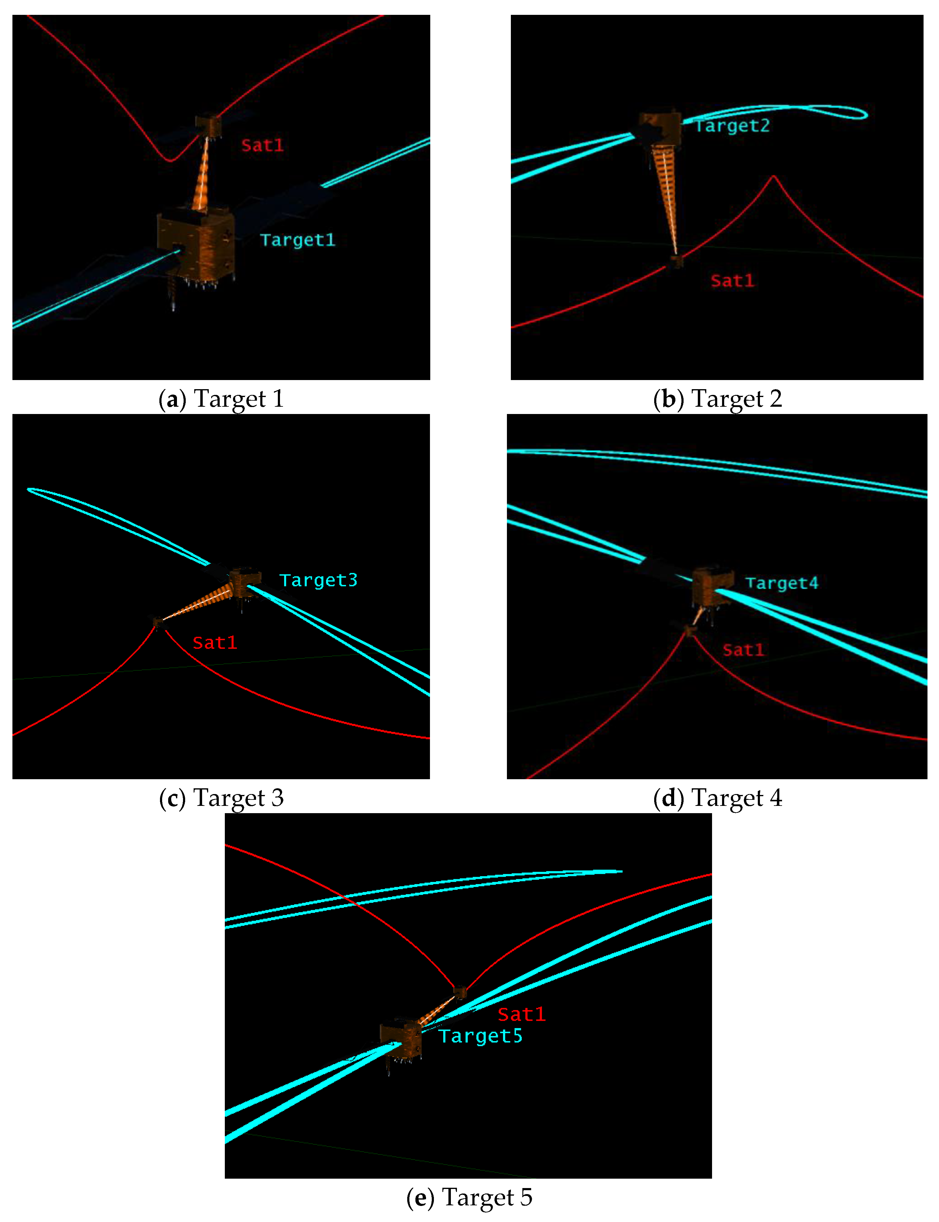
| Target | 1 | 2 | 3 | 4 | 5 |
|---|---|---|---|---|---|
| Minimum patrol distance (km) | 108.8 | 187.1 | 205.7 | 84.7 | 101.1 |
| Patrol duration (s) | 5820.6 | 1180.5 | 1585.7 | 1487.6 | 1352.9 |
Disclaimer/Publisher’s Note: The statements, opinions and data contained in all publications are solely those of the individual author(s) and contributor(s) and not of MDPI and/or the editor(s). MDPI and/or the editor(s) disclaim responsibility for any injury to people or property resulting from any ideas, methods, instructions or products referred to in the content. |
© 2025 by the authors. Licensee MDPI, Basel, Switzerland. This article is an open access article distributed under the terms and conditions of the Creative Commons Attribution (CC BY) license (https://creativecommons.org/licenses/by/4.0/).
Share and Cite
Chen, N.; Zhang, Z.; Feng, S.; Xue, W.; Jia, B. A Patrol Route Design for Inclined Geosynchronous Orbit Satellites in Space Traffic Management. Aerospace 2025, 12, 299. https://doi.org/10.3390/aerospace12040299
Chen N, Zhang Z, Feng S, Xue W, Jia B. A Patrol Route Design for Inclined Geosynchronous Orbit Satellites in Space Traffic Management. Aerospace. 2025; 12(4):299. https://doi.org/10.3390/aerospace12040299
Chicago/Turabian StyleChen, Ning, Zhanyue Zhang, Songjiang Feng, Wu Xue, and Boya Jia. 2025. "A Patrol Route Design for Inclined Geosynchronous Orbit Satellites in Space Traffic Management" Aerospace 12, no. 4: 299. https://doi.org/10.3390/aerospace12040299
APA StyleChen, N., Zhang, Z., Feng, S., Xue, W., & Jia, B. (2025). A Patrol Route Design for Inclined Geosynchronous Orbit Satellites in Space Traffic Management. Aerospace, 12(4), 299. https://doi.org/10.3390/aerospace12040299