1. Introduction
Atmospheric turbulence, inducing civil aviation aircraft bumpiness, is by far the leading cause of aircraft damage and passenger and crew injuries [
1,
2]. Before conducting a scheduled civil aviation flight, the airline’s operation and control department needs to analyze various meteorological information and develop a flight plan to prevent serious aircraft bumpiness and potential hazards. However, analyses and forecasts based on meteorological data cannot completely avoid the occurrence of aircraft bumpiness and injuries. As a traditional turbulence observation, pilot reports (PIREPs) are not suited to provide reliable turbulence severity since the subjective PIREP can only be interpreted by the flight crew [
3,
4]. Several quantitative turbulence observations based on flight data, like the vertical acceleration (VA), the derived equivalent vertical gust velocity (DEVG), and eddy dissipation rate (EDR), support the construction of the turbulence maps within the target airspace, providing better tactical avoidance options for civil aviation aircraft. As an in situ reporting indicator, the VA indicator was first put forward since turbulence severity is proportional to the root-mean-square of aircraft vertical acceleration [
5]. Compared with the VA, the DEVG indicator was further related to aircraft mass and airspeed, but it cannot be regarded as an objective severity metric as well [
6,
7]. To obtain the aircraft-independent turbulence severity, the EDR indicator has been the turbulence severity metric of the aircraft meteorological data relay (AMDAR) standard required by the International Civil Aviation Organization (ICAO) [
8,
9,
10].
Based on the observed vertical wind or aircraft vertical acceleration from flight data, the EDR indicator gives an objective and aircraft-independent indication of turbulence severity theoretically. In the acceleration-based EDR algorithm, turbulence severity was recovered from aircraft vertical acceleration response; thus, the acceleration response to turbulence is fundamental to EDR estimation [
11]. In turbulent flight, aircraft plunge and pitch motions, providing the largest contribution to vertical acceleration, were characterized by linear transfer function models, respectively. Taking the wind effects as the only excitation of interest, a quasi-static aerodynamic model and control surface-fixed assumptions were made in the derivation of a linear model. However, it is difficult to recover the objective turbulence severity because the linear model cannot describe the nonlinear and high-frequency acceleration response in turbulent flight accurately. Furthermore, the control surface deflections, not characterized in the linear model, could induce the acceleration change as well [
12]. Another major concern is the determination of the bandpass filter, which is concatenated to the response function to eliminate the influence of aircraft maneuvering and high-frequency structural vibration. In fact, the passband range determines the turbulence frequencies that induce the aircraft bumpiness.
On the other hand, the vertical wind-based EDR algorithm is able to derive the objective turbulence severity based on the maximum likelihood estimation (MLE) in the frequency domain. By exemplifying the derivation of acceleration response and deriving the vertical component of turbulence from six flight variables directly, the wind-based EDR algorithm provides a much more objective turbulence severity indicator than the acceleration-based algorithm [
13]. Unfortunately, the length scale change in turbulence is not considered, thus leading to the empirical selection of the integration range in maximum likelihood estimation [
14].
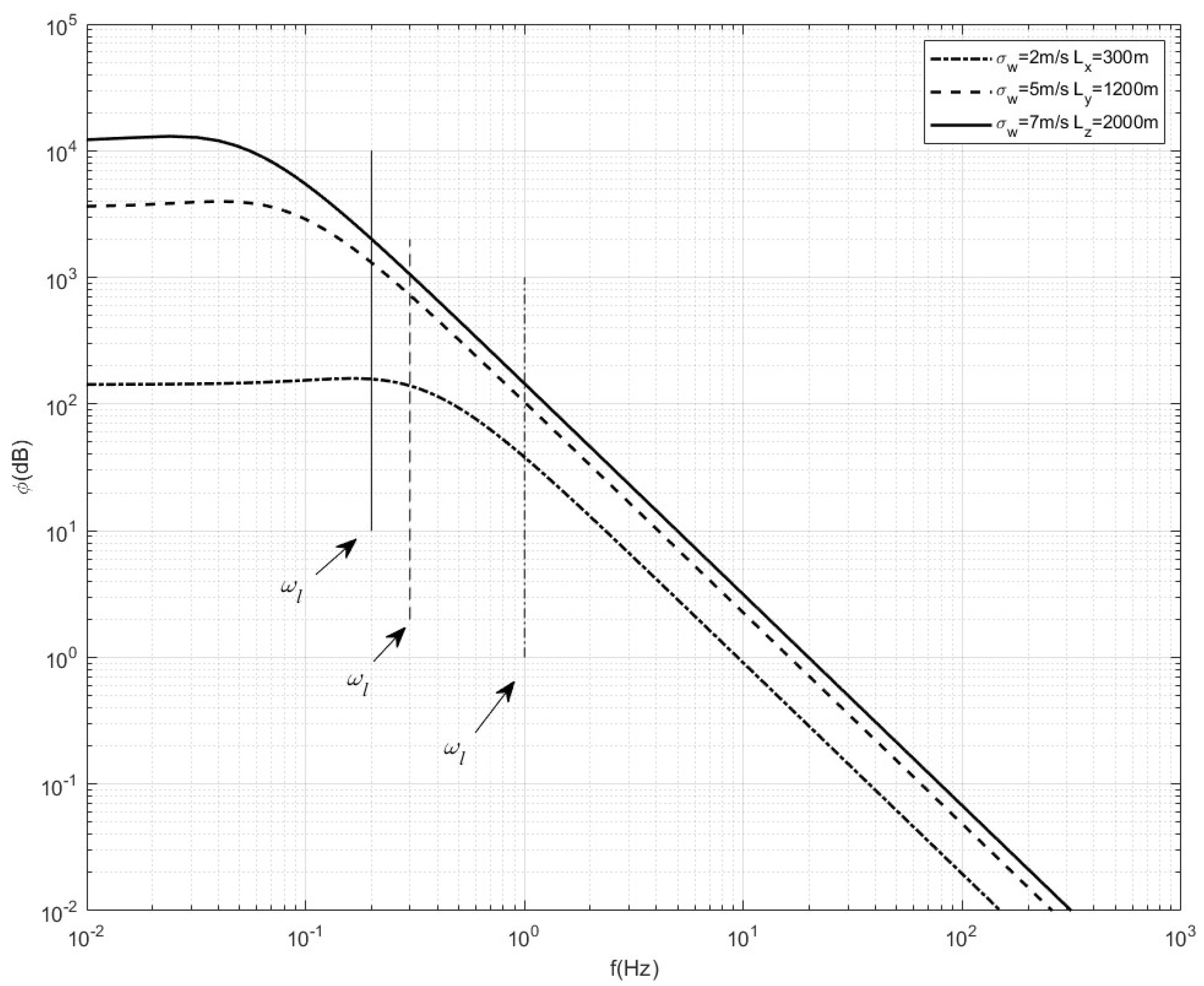
Not only the passband range in acceleration-based EDR estimation but also the integration range in the wind-based EDR algorithm depend on the determination of the turbulence inertial subrange. In fact, aircraft acceleration change is affected by a certain wavelength range of turbulent eddies [
15,
16]. The turbulent eddies in this particular range are felt by the aircraft as bumpiness. For most commercial aircraft, this size range forms the inertial subrange, covering from approximately 10 m to 1000 m [
17]. According to the Kolmogorov hypothesis, the turbulent energy is neither produced nor dissipated, but is transferred from larger to smaller eddies in this subrange inertially. Within the inertial subrange, the energy spectrum only depends on the EDR, showing a −5/3 power law in turbulence spectrogram, thus forming the basis of both EDR algorithms. Only within the inertial subrange can the passband range or integration range be determined quantitatively; thus, the determination of the inertial subrange has major effects on the algorithm accuracy. Unfortunately, the inertial subrange in current EDR algorithms is selected empirically. Taking the flight data with a sampling rate of 8 Hz as an example, only the frequencies within 4 Hz are available according to the Nyquist sampling theorem. The frequencies below 0.5 Hz are filtered out because of a possible error. In addition, the upper range from 3.5 Hz to 4 Hz is excluded as well since there may exist contamination from noise and sampling artifacts. As a result, a frequency range of 0.5 Hz to 3.5 Hz is determined empirically. Taking an aircraft flying at an airspeed of as an example, the frequency range covers 0.5 Hz to 250 Hz. To obtain the EDR indicator with better accuracy, the inertial subrange of the EDR algorithm needs to be characterized quantitatively.
Compared with the EDR indicator as an objective turbulence severity metric, estimating bumpiness severity related to a specific aircraft brings airlines substantial benefits. In flying through the same turbulence field, different aircraft would experience different bumpiness severities. Based on the objective EDR indicator, the accurate estimation of aircraft response to turbulence is still fundamental to obtain the aircraft-dependent bumpiness. Compared with the linear response model, it holds promise to obtain the acceleration response with better accuracy by using the vortex lattice method (VLM). As a typical numerical algorithm of linear potential flow theory, the VLM is highly practical and widely used in aerodynamics studies. In VLM, the lifting body is characterized by a limited number of discrete horseshoe vortices attached to the surface. In the earliest application of VLM in exploring wind disturbance effects, the lifting body was simplified as a planar surface. In addition, the two semi-infinite vortex filaments in steady VLM have difficulty in characterizing the unsteady flight state change [
18,
19].
As the extension of VLM, the ring vortex is composed of quadrilateral vortex segments in a closed loop. With dozens of ring vortices distributed on the camber surface of the lifting body, the solving accuracy of VLM is improved. Furthermore, based on the ring vortex element, basic VLM is directly extended to nonstationary situations, giving rise to the time-domain unsteady vortex-lattice method (UVLM). The UVLM has been gaining ground in situations where free-wake methods become a necessity [
20,
21]. With the advent of novel lifting body configurations and increased structural flexibility, the UVLM constitutes an attractive solution for aircraft dynamics problems, including the computation of stability derivatives [
22,
23], flutter suppression [
24,
25], gust response [
26,
27], morphing vehicles [
28,
29], and coupled aero-elasticity and flight dynamics [
30,
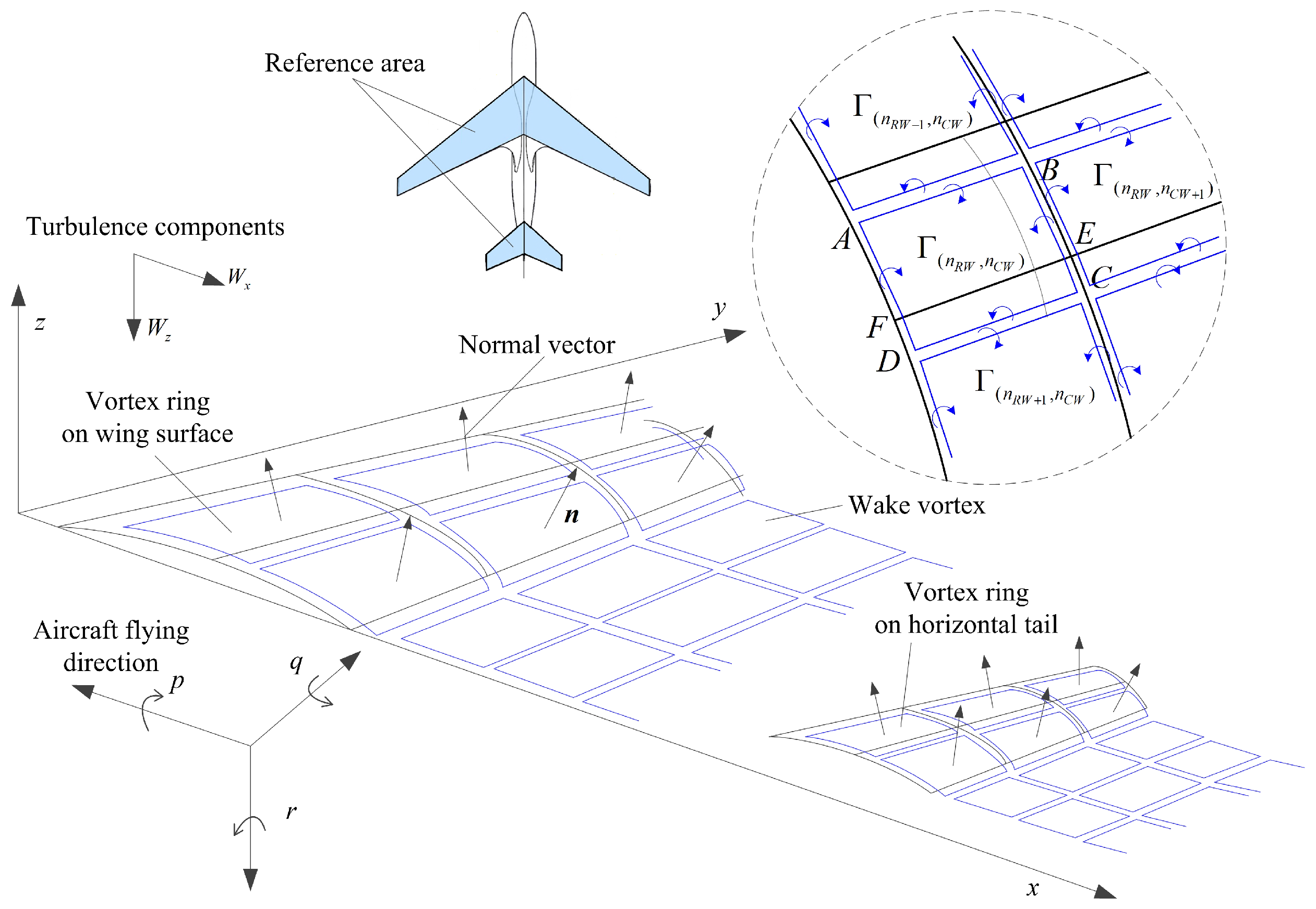
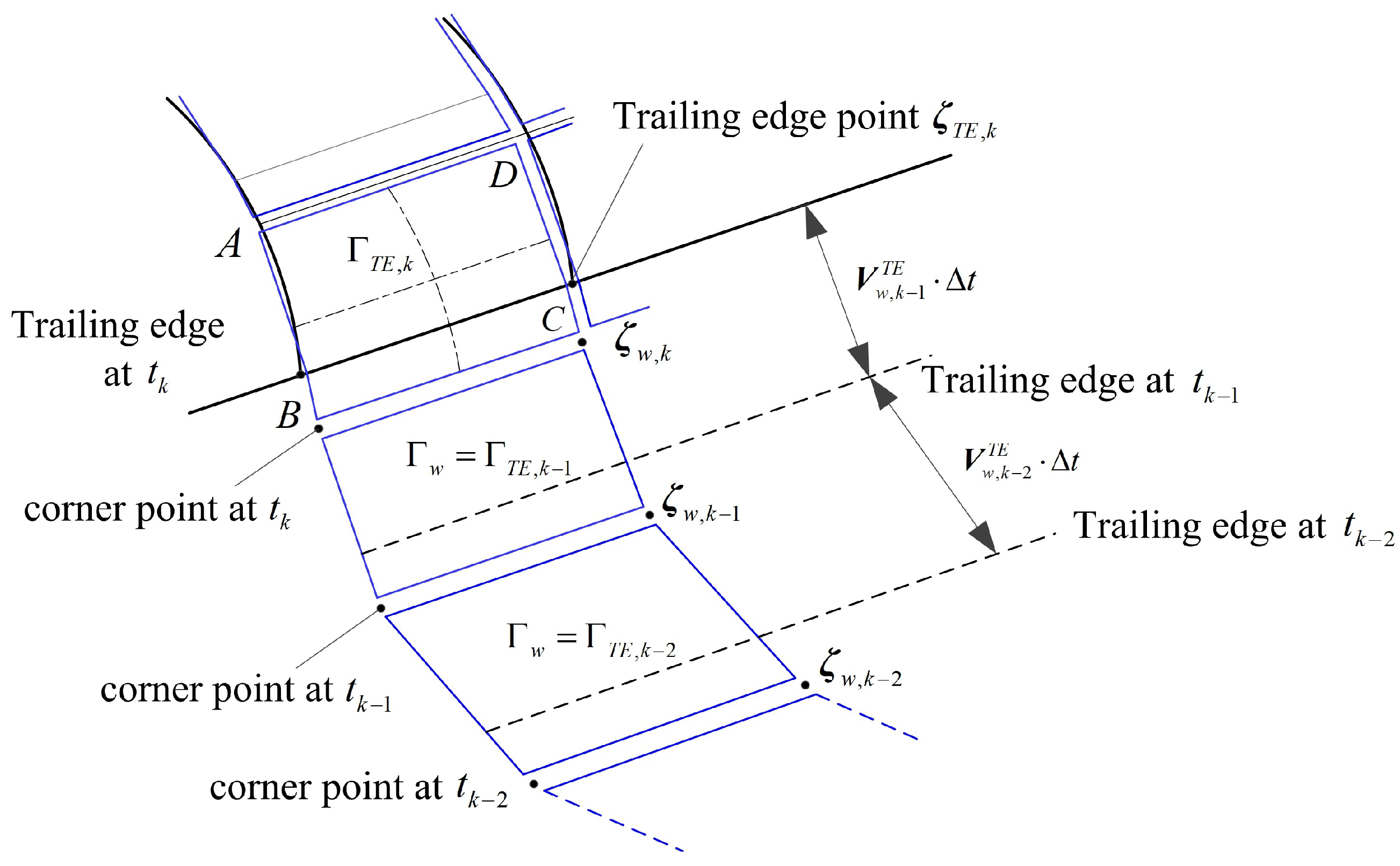
31]. In turbulent flight, lifting surfaces and wakes can be discretized using ring vortices, and the wake vortex rings are freely convected according to the local flow velocity, developing into a force-free wake system. During the subsonic cruising flight of civil aviation aircraft, the airflow can be regarded as inviscid since the Reynolds number is large enough and the flow remains attached [
32]. Therefore, based on full potential equations without any linearization, the UVLM is able to well reflect the unsteadiness effects of the turbulent airflow around the aircraft, and the acceleration response of the aircraft in turbulence is obtained with better accuracy.
This study contributes to the optimization of the inertial subrange in the objective wind-based EDR algorithm and the aircraft-dependent bumpiness estimation based on UVLM. The effect of the inertial subrange on the EDR algorithm is characterized first. After determining the minimum series length for the EDR algorithm under a certain flight data sampling rate, an optimized inertial subrange is determined by extending the series to achieve an acceptable variance of spectrum estimation. Furthermore, the acceleration response to turbulence is characterized by deriving a time-marching UVLM in turbulent wind. After this, an aircraft bumpiness nowcast and bumpiness forecast algorithm are derived successively. By simulation study and tests on airway flight data, the inertial-subrange-optimized EDR algorithm and the aircraft-dependent bumpiness estimation algorithm are tested and discussed in depth.
3. Results and Discussion
In this section, the aircraft-independent EDR estimation and aircraft-dependent bumpiness estimation are explored by simulation and experiment based on real flight data. The flight data sets of civil aviation aircraft flying from Chengdu Shuangliu Airport (ZUUU) to Lhasa Kongga Airport (ZULS) of China were collected. A data set of 3127 flights was gathered, covering April 2019 to April 2023. Of these, the Airbus A319 and A330 are two main aircraft types. Combined with the strong solar radiation and complex highland terrain, the turbulence area under the tropospheric jet axis could induce severe aircraft bumpiness. Based on the flight data set of ZUUU-ZULS, twenty wind scenarios (S1–S20) covering light, moderate, and severe turbulence are sampled and recorded. In this study, eight scenarios are used to test the acceleration response and estimate aircraft bumpiness, as shown in
Table 2.
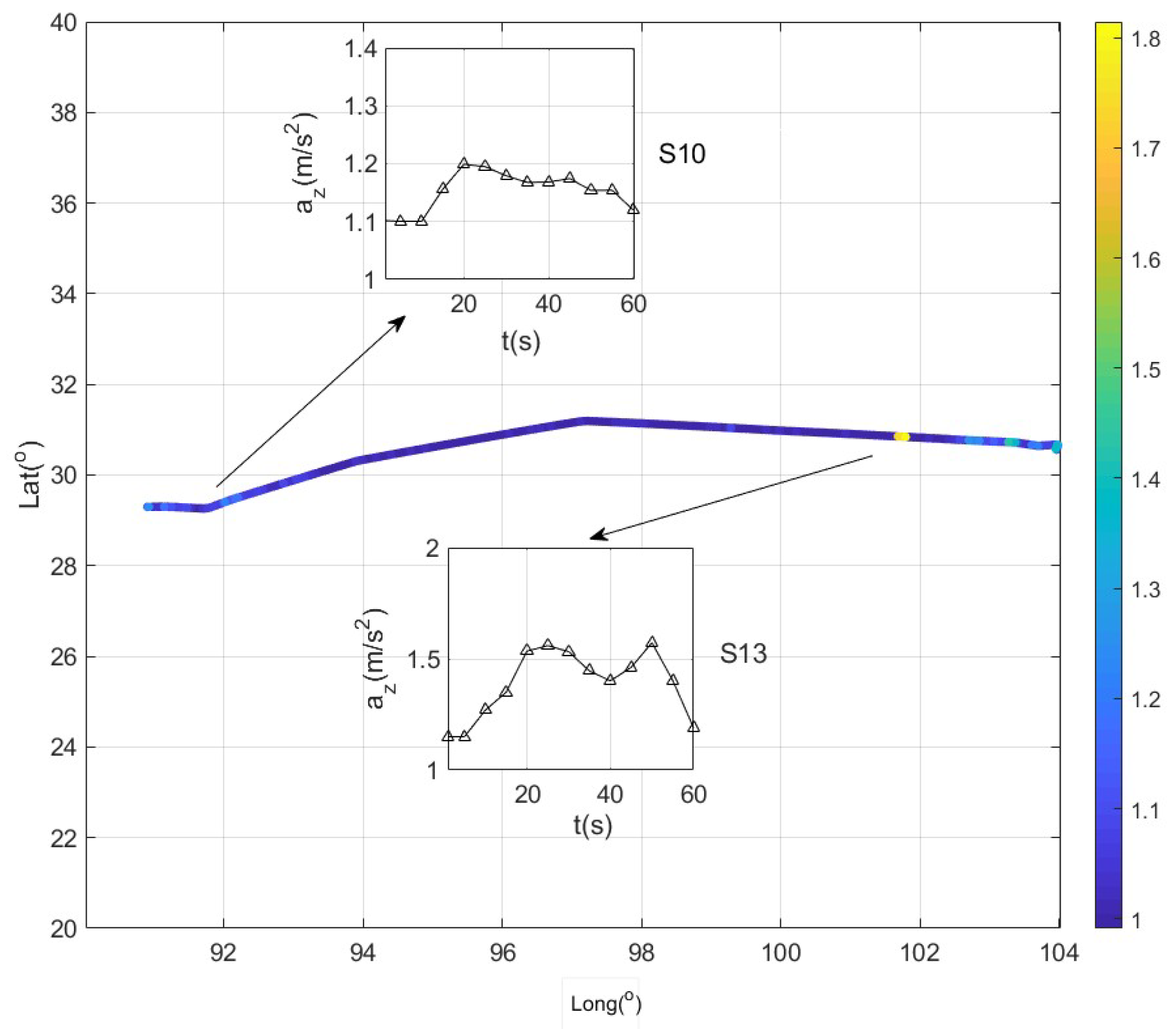
Two scenarios, S10 and S13, are used for vertical acceleration analysis, as shown in
Figure 6. S13 is located at 101.75 east longitude (101.75 E) and 30.85 north latitude (30.85 N). The aircraft A319 experienced severe bumpiness with maximum acceleration
g. After that, the later aircraft flew around this zone. S10 is located at 92.25 E and 29.5 N. The A319 experienced moderate bumpiness with maximum acceleration
g. After 9 min, another A330 flew across this zone and experienced the turbulence. It should be noted that the vertical acceleration cannot reflect the objective turbulence severity because different aircraft with different weights and airspeeds would experience different acceleration responses.
3.1. The Optimized Aircraft-Independent EDR Estimation
3.1.1. The Determination of Minimum Series Length for EDR Estimation
Under a certain sampling rate of flight data, the minimum series length of EDR estimation was determined. After this, the inertial subrange was obtained by reducing the variance of spectral estimation. A simulation test was performed to determine the minimum sequence length for EDR estimation under a certain sampling rate of flight data. On the one hand, a spatial 3-D Fourier transform was leveraged to generate the vertical component of turbulence series conforming to the von Kármán model [
44]. With several kinds of turbulence intensities and length scales, different EDR values were estimated according to Equation (
8). On the other hand, the corresponding theoretical EDR values are able to be obtained by using Equation (
6). As a result, the estimation quality under different series lengths was compared with the theoretical EDR value through statistical analysis.
Taking turbulence sampling rate
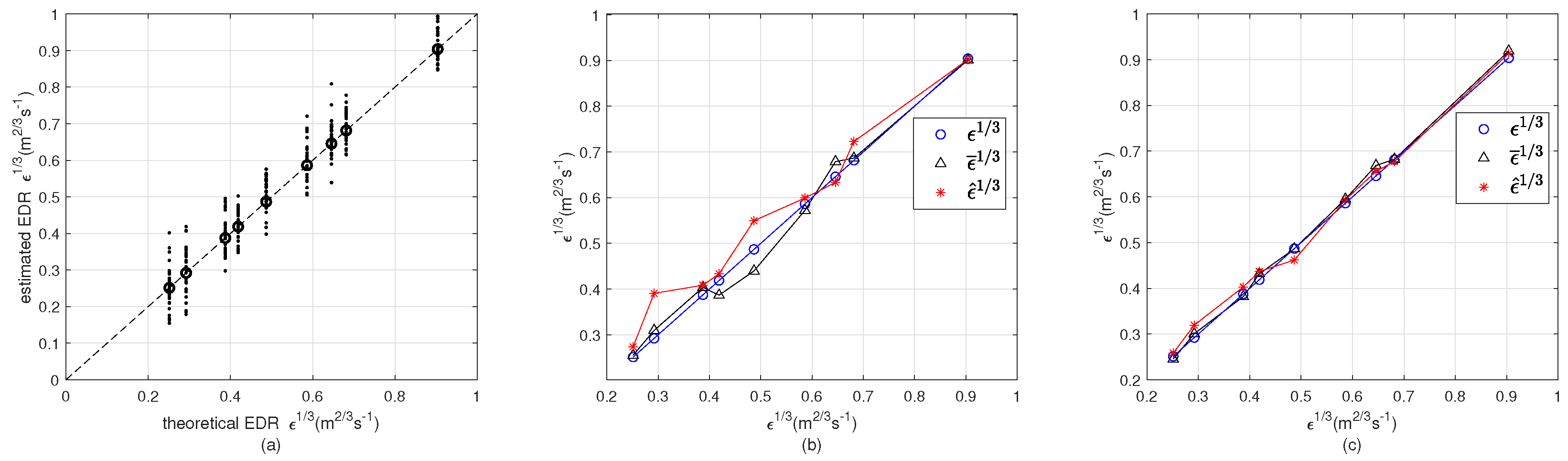
Hz as an example, three different turbulence intensities covering light, moderate, and severe circumstances, and three different length scales were selected to constitute nine groups of turbulence series, forming nine test conditions (TC), as shown in
Table 3. The turbulence series was further divided by
segments, while in each segment the series length
. As shown in
Figure 7a, the nine circles indicate the theoretical
, while the estimated EDR values are distributed around the theoretical values.
By numerical simulation, 100 × 9 = 900 EDR values were generated, and the consistency test was further performed. For each TC, the average value
and the estimated value
are both shown in
Table 3. With initial setting
, the interclass correlation coefficient ICC = 0.7731. This low ICC value indicates that an accurate and stable EDR value cannot be obtained under the series length
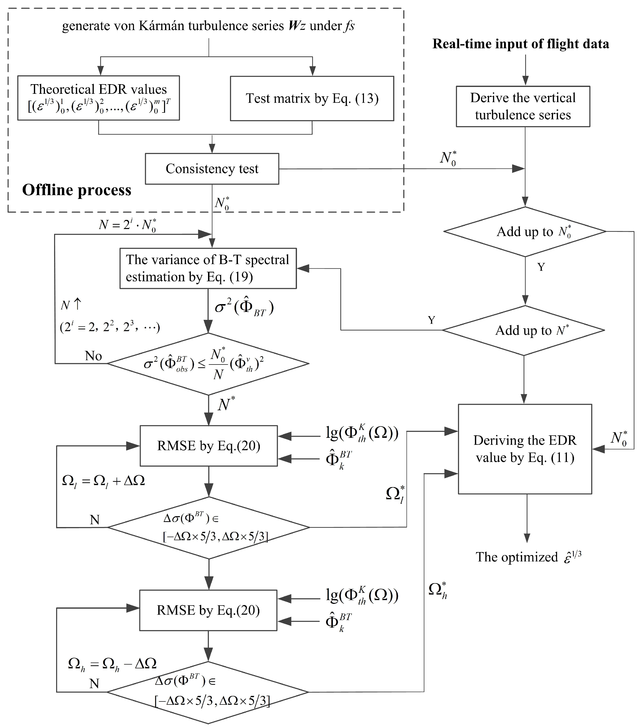
. According to the algorithm flow in
Figure 3, by extending the series length to
and carrying out the simulation and consistency test again, the ICC value was increased to ICC = 0.9312.
Figure 7b shows the
and
corresponding to each TC under
, while
Figure 7c shows the two variables under
.
3.1.2. The Optimization of Inertial Subrange
By the analysis above, the minimum series length to estimate the EDR value is
with the sampling rate
. According to Equation (
19), the Hanning window function with width
was applied, and
. Thus, the variance of spectral estimation is poor based on the minimum series. By referring to Blackman–Tukey spectra estimation theory, a longer series length for optimizing the inertial subrange is determined by extending the series with power 2. By iterations, the series length was extended to
, thus leading to an acceptable variance. Based on the proposed method,
Table 4 shows the variance change in the nine TCs before and after series extension.
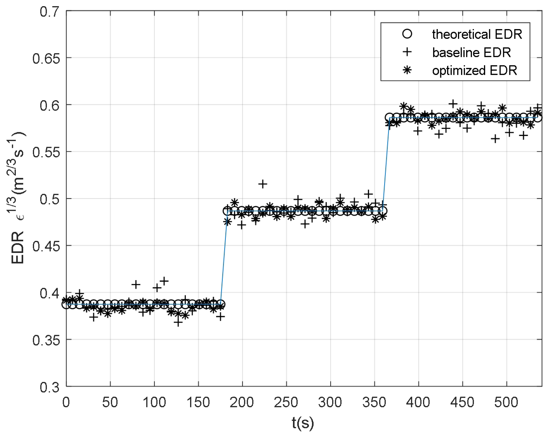
The optimization of the inertial subrange is tested by changing of turbulence intensity and length scale intermittently in the simulation. The turbulence series was set initially by
m and
m/s. At 3 min, the parameters are changed by
m and
m/s. At 6 min, the parameters are changed by
m and
m/s. Under the sampling rate
, the EDR estimation is carried out every 256 points, namely 8 s. Besides, the inertial subrange is optimized every 2048 points, that is, 64 s. By optimization, the inertial subrange at 64 s, 256 s, 448 s is estimated by [0.9, 20.0], [0.5, 18.3], [0.4, 14.6], respectively, as shown in
Figure 8.
The theoretical EDR value, the baseline EDR value with default fixed inertial subrange, and the derived EDR value under the optimized inertial subrange are shown in
Figure 9. The mean squared error (MSE) of baseline EDR is
, while the MSE of optimized EDR is
. It can be found that the EDR estimation with the inertial subrange optimized is more stable than the traditional EDR estimation.
3.1.3. The Optimized Aircraft-Independent EDR Estimation Based on Flight Data
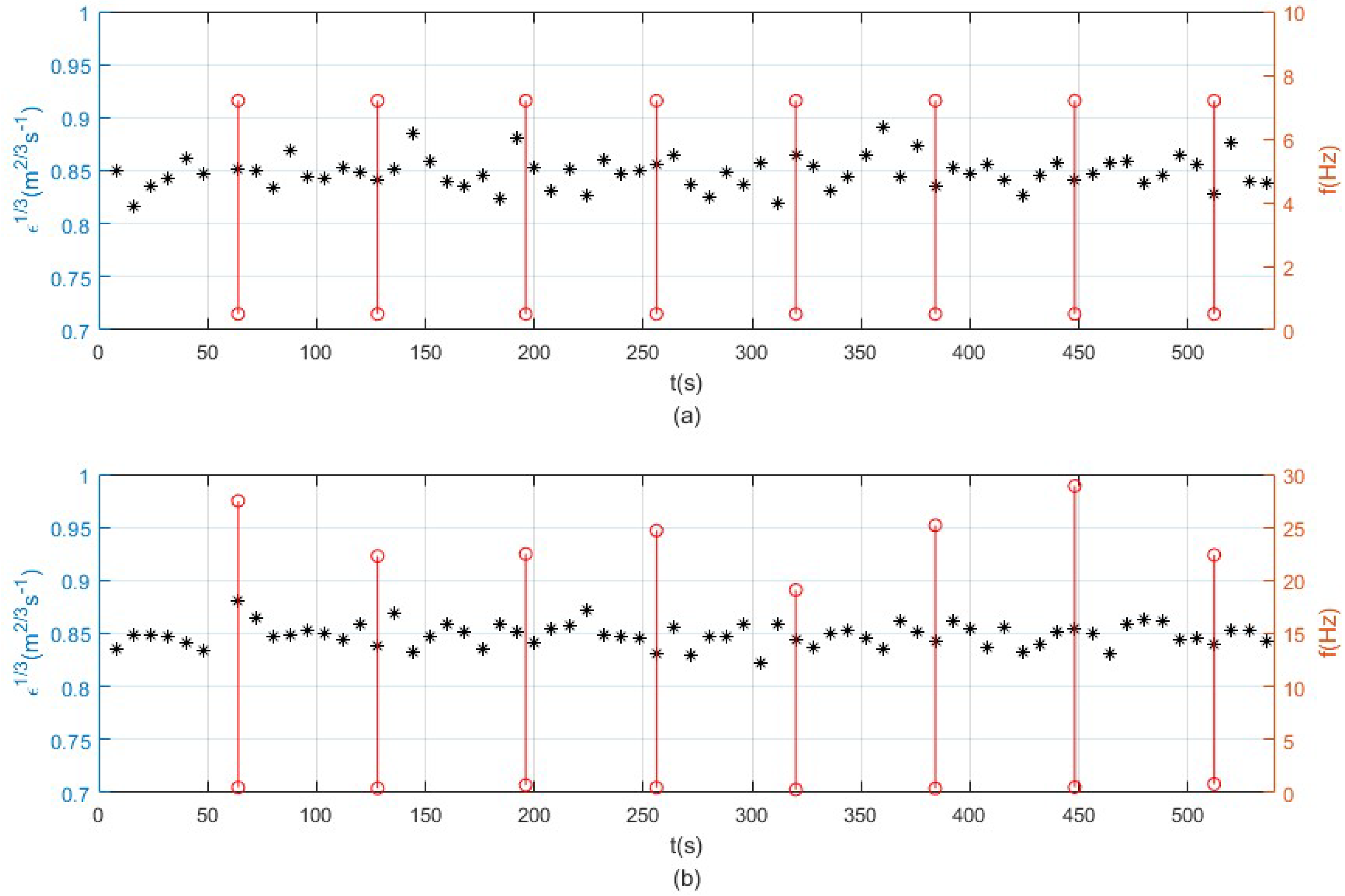
According to the ZUUU-ZULS flight data sets, the optimized aircraft-independent EDR estimation of the two scenarios was performed successively. S13 with severe turbulence was analyzed first. After experiencing severe bumpiness, the following aircraft deviated from this zone. According to the flight data sampling rate of 16 Hz, the minimum series length for EDR estimation is
. To improve the variance performance, the extended series length is
. As a result, the EDR estimation is carried out every 128/16 = 8 s, while the inertial subrange optimization is carried out every
s. In nine minutes, the change in inertial subrange marked by red lines is shown in
Figure 10, showing the inertial subrange at 64 s, 128 s, 196 s, 256 s, 320 s, 384 s, 448 s, and 512 s successively.
The EDR estimation results of baseline (in
Figure 10a) and inertial subrange-optimized EDR estimation (in
Figure 10b) are shown in
Figure 10 as well. The default inertial subrange [0.5, 7.2] was applied to basic EDR estimation. Compared with the simulation test in
Section 3.1, we cannot provide the theoretical EDR value. By observation, the stability of inertial subrange-optimized EDR estimation is better than that of the basic EDR estimation, which is consistent with the theoretical analysis.
At S10, the two aircraft flew through moderate turbulence with a time lag of about 9 min. The turbulence parameters are assumed to be unchanged for 9 min under the assumption of a frozen field. According to the flight data of two aircraft, the inertial subrange and EDR value are derived.
Table 5 shows the inertial subrange estimation by the two aircraft. The inertial subranges estimated by A319 and A330 at each time point are similar.
Figure 11 shows the EDR estimation by A319 and A330, respectively. The estimated results of both aircraft are similar. Therefore, the inertial subrange-optimized EDR estimation is effective.
Figure 12 shows the optimized EDR estimation results observed by A319. The EDR value of the two zones is shown in two subwindows, from which it can be found that the objective EDR value is different from the vertical acceleration, as shown in
Figure 6.
3.2. The Aircraft-Dependent Bumpiness Estimation
3.2.1. The Acceleration Response to Turbulence
Accurate acceleration response forms the basis of deriving aircraft-dependent bumpiness severity. The effectiveness of UVLM, including the grid number refinement and the steady aerodynamic test, was tested with the Boeing 737-800 aircraft [
45]. The algorithm had been proven to track the continuous change in aircraft normal acceleration. Though there exist a few deviations in peak acceleration response, UVLM performed a good sensitivity to severe turbulence, resulting in an over-prediction of peak values.
In addition to the acceleration change induced by atmospheric disturbance, pilots’ manipulation would cause control surface deflections, thus leading to acceleration change as well. With the FDMs of A319 and A330 aircraft integrated, this study focused on the separation of aircraft maneuvers by UVLM. The results of UVLM are compared with recorded flight data. The force-free wake vortex was applied to compute the continuous response to turbulence. The turbulence input was derived from flight data by referring to [
9]. To carry out the UVLM, the wing–tail assembly model of the Airbus A319 and A330 is built first.
Table 6 lists the geometric parameters and grid divisions of A319 and A330 aircraft.
To deal with aircraft bumpiness in turbulence, the acceleration change induced by aircraft maneuvers must be separated from the acceleration response. Taking the A319 as an example, the aircraft maneuvers induced by both control surface deflections and the effects on acceleration response were studied.
Figure 13 shows the test results of S11, where the aircraft encountered continuous and low-amplitude turbulence disturbance. The longitudinal and vertical turbulence components are shown in
Figure 13a.
Figure 13b,c show the elevator and spoilers deflected by automatic flight control or manual manipulation in order to suppress the aircraft bumpiness. As shown in
Figure 13d, the aircraft encountered severe bumpiness during 50 s–60 s. At 58 s, the aircraft encountered the vertical wind of −10 m/s. After a while, the vertical wind changed suddenly to 13 m/s. The elevator deflected quickly, and the high-speed and low-speed spoilers deflected after a short delay. In
Figure 13d, the red curve depicts the series
, showing the acceleration change induced by turbulence solely. The series is obtained by carrying out UVLM twice. Firstly, the series
is generated by inputting turbulence and control deflections. After that, the series
is computed only with control deflections. From the vertical acceleration response, the effect of control surface deflections on acceleration change can be observed. Results indicate that the adverse effects of control surface deflections can be separated by performing UVLM twice.
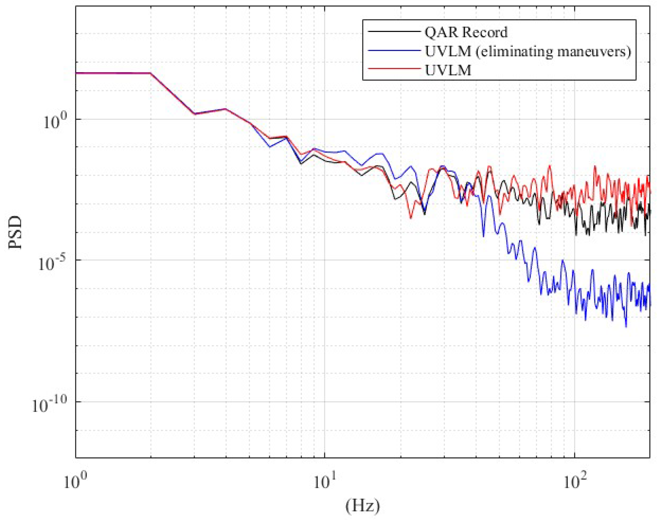
The spectra of computed acceleration and recorded value are compared as shown in
Figure 14. It shows that the UVLM is able to track the fluctuation better in the high-frequency domain. However, with aircraft maneuvers eliminated, the total energy of the acceleration spectra is smaller than that of the recorded acceleration. It can be concluded that the vertical acceleration change is not only induced by turbulence, but also affected by aircraft maneuvers, in other words, the deflections of control surfaces. Since the boundary of the vortex lattice was designed to approximate the structural boundary of control surfaces, the acceleration induced by aircraft maneuvers can be separated from that induced by turbulence.
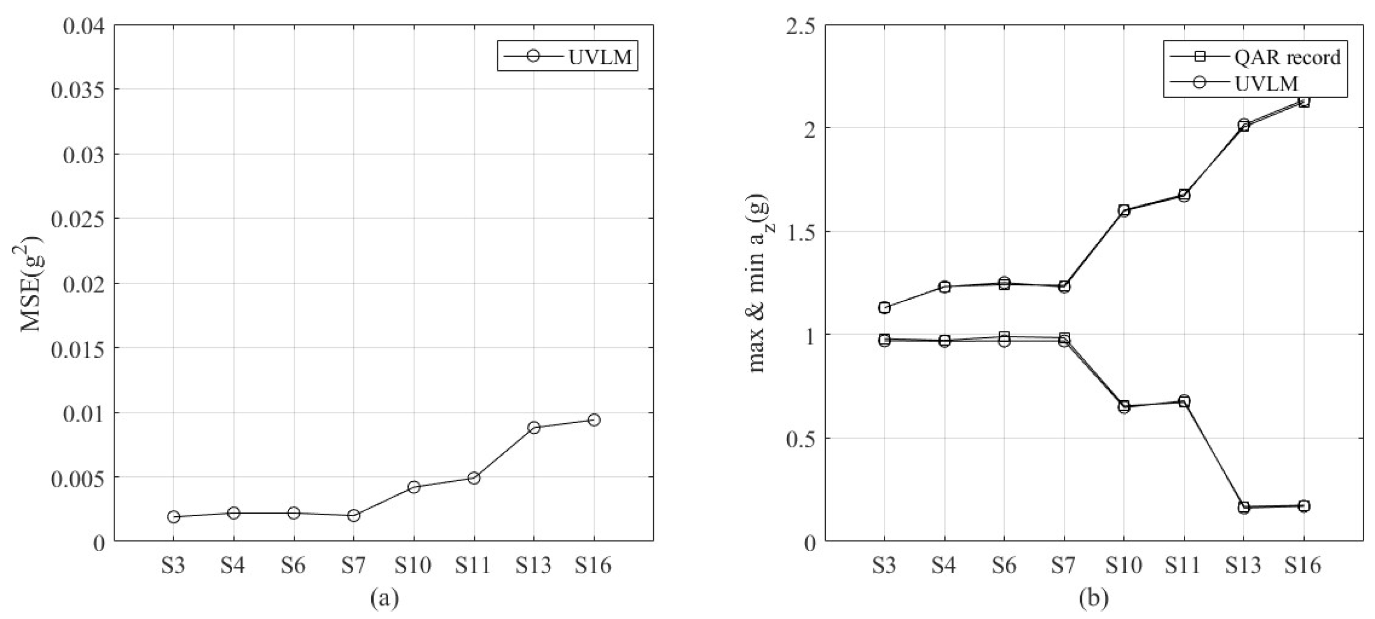
The MSE and peak acceleration of the eight wind scenarios are compared as shown in
Figure 15. UVLM shows better computing accuracy in varied turbulence severities. With the increase in turbulence severities, the MSE increases. However, the maximum MSE is less than 0.01, and the peak acceleration can fit the recorded flight data well.
3.2.2. In Situ Aircraft-Dependent Bumpiness Estimation Based on Flight Data
Taking the S10 as an example, the aircraft-dependent in situ bumpiness estimation and prediction are tested, respectively. The in situ aircraft bumpiness estimation is performed in S10 to test the bumpiness difference in different aircraft. Based on the algorithm of
Table 1, the in situ aircraft bumpiness estimation in S10 is shown in
Figure 16. The bumpiness severity of A330 is lower than that of A319. The estimated results are consistent with the recorded vertical acceleration, which is mixed with control surface deflection-induced maneuvers.
3.3. Further Discussion
The turbulence components, the wave number of which lies in the inertial subrange, have direct effects on aircraft bumpiness. Different sampling rates would have major effects on the selection of the inertial subrange. This study proposes an effective way of searching the inertial subrange under different sampling rates. The selection of the inertial subrange is not only helpful to obtain the objective EDR estimation with better accuracy, but also fundamental to obtain the aircraft-dependent bumpiness.
The accurate computation of vertical acceleration is fundamental to obtain aircraft-dependent bumpiness. Compared with the linear model based on small perturbation theory, the proposed method based on linear potential theory is helpful to track the peak vertical acceleration with better accuracy. In addition, it is reported that a pilot’s incorrect manipulation would deteriorate aircraft bumpiness in severe turbulence [
46]. Since the vertical acceleration is generated by either turbulent wind or control surface deflection, the linear potential method is capable of separating the aircraft maneuver effects from the vertical acceleration. The proposed method can be further applied to aircraft bumpiness analysis. To reduce the bumpiness severity, the control surfaces may be deflected under the control of the automatic flight control system in turbulent flight. Therefore, it is necessary to consider the influence of control surface deflection. In UVLM, aerodynamic control surfaces can be directly modeled by prescribed deflections of trailing edge panels and the corresponding rotation of normal vectors. Therefore, the UVLM-based acceleration analysis is helpful to investigate the bumpiness induced by turbulence.
Aircraft-related bumpiness can be obtained with an optimized inertial subrange. In fact, two aircraft penetrating the same turbulence field at different speeds may experience quite different disturbances. An aircraft-related bumpiness estimation is tested based on the flight data from A319 and A330 aircraft. It should be noted that if the computing results of target aircraft are saved into a table beforehand according to different aircraft mass and airspeed, the bumpiness severity of target aircraft can be estimated by looking up the table with the in situ EDR value. In addition, the bumpiness severity of the aircraft that is about to fly through the turbulence field can also be predicted.
After this, the aircraft bumpiness prediction is performed in S13. The predicted aircraft bumpiness can be used to judge whether the following aircraft can fly through a turbulence field or not. Based on the frozen field assumption, in the same turbulence field, different aircraft would experience different turbulence severities. Therefore, the objective EDR value cannot be regarded as the actual bumpiness indicator. With the increase in aircraft weight, the bumpiness severities reduce. In addition, with the increase in airspeed, the bumpiness severities increase. The A319 and A330 aircraft bumpiness prediction in S13 is shown in
Figure 17. According to different aircraft weight and airspeed, the bumpiness severity of the target aircraft can be calculated and saved in the database. Then, the bumpiness severity can be obtained by table look-up. According to the predicted EDR indicator, the flight crew can decide whether to fly through or deviate severe turbulence area. On the other hand, the objective turbulence severity can be derived from post hoc flight data. Thus, the following aircraft bumpiness can be predicted by the algorithm.


