A Two-Stage Optimization Method for Multi-Runway Departure Sequencing Based on Continuous-Time Markov Chain

Abstract

With the rapid expansion of the aviation industry, traditional static scheduling methods have become inadequate to meet the increasingly complex demands of efficient airport operations. To enhance the operational efficiency of multi-runway airports, this paper introduced a two-stage dynamic departure scheduling method based on continuous Markov chains. The pushback rate control strategy was extended to multi-runway scenarios to identify the optimal taxiway queue threshold in stage I. In stage II, the pushback rate control strategy with a known queue threshold was introduced into a multi-objective optimization model, aiming to minimize flight delays and operational costs including pushback waiting times, taxi fuel consumption, and environmental impact. Then, continuous-time Markov chains (CTMC) were employed to track aircraft state transitions in the taxiway queue, and a nested whale optimization algorithm was proposed to optimize both the pushback sequence and runway resource allocation. Results indicate that the proposed method reduced the average taxiway queue time by 55.58%, with delay reductions of up to 73.06%, offering significant cost savings and environmental benefits while improving flight punctuality. This innovative approach highlights the potential for optimizing airport resource scheduling in complex and dynamic environments.

1. Introduction

Amid the rapid development of modern air transportation, airports, as pivotal nodes in the aviation network, play a crucial role in determining the overall efficiency of the aviation system and exert a direct impact on both the passenger experience and environmental sustainability. The rising demand for air transport has made the limited capacity of airports a significant constraint on the development of civil aviation. In many major airports worldwide, such as London Heathrow, capacity constraints have persisted for decades, further exacerbated by local opposition to expansion projects [1]. For most airports globally, the limitation has become increasingly pronounced, especially as flight volumes remain at consistently high levels, reducing the safety margins and challenging airport surface operational efficiency. From a hardware perspective, some hub airports have taken measures such as adding additional runways, but the conflict between demand and capacity remains unresolved. In terms of management, the increasing complexity of airport ground operations, coupled with the continuous growth in flight traffic, has rendered traditional flight scheduling methods inadequate to meet the current demands.

To alleviate this pressure, the optimization of single airport resources has been extensively studied. Among them, effective pushback control strategies can significantly reduce taxi delays and minimize fuel consumption. The introduction of Markov chains, in particular, when modeling taxiways as queuing systems, has further advanced the depth of this research [2]. Nevertheless, these models do not explicitly consider runway service times; moreover, plenty of approaches remain untested in multi-runway systems, where the coordination of multiple departure queues presents new challenges. The next critical step in optimizing airport departure processes lies in sequencing departing flights and assigning runways. Current research typically constructs optimization models aimed at minimizing flight delays and maximizing runway throughput in airport operations, employing various algorithms for flight scheduling [3], notably with a significantly greater focus on arrival procedures compared with departures.

Meanwhile, due to the increased demand for flights, flight fuel consumption and emissions also face challenges [4]. Data indicate that carbon dioxide emissions from the aviation industry account for 12% of all transportation-related emissions and approximately 2.9% of the total global emissions [5,6]. However, hub airports with multiple runways and gates face significant operational uncertainties during ground operations, and inefficient resource allocation can extend the ground operation times and increase environmental gas emissions [7]. Thus, in the context of high-density airport operations, the development of a dynamic cooperative scheduling method that aligns with the characteristics of multi-runway airports is of significant theoretical and practical value for optimizing ground operations, enhancing flight punctuality and promoting green and sustainable development. To address this challenge, this paper proposed an innovative dynamic scheduling method for departing flights, with a primary focus on the coordinated optimization of the pushback and sequencing assignment processes. By aligning with the operational demands of airports and considering the dynamics and complexity of ground operations, we aimed to enhance the efficiency of multi-runway airports under mixed take-off and landing conditions. The method can be divided into two stages: the first stage extends the pushback control strategies across multiple runways to determine the optimal thresholds, reducing the taxiway waiting times and alleviating congestion; the second stage, which is the core of the method, is dedicated to the integration of flight sequencing and runway assignment, using a multi-objective optimization model to minimize flight delays and operational costs. By embedding a continuous-time Markov chain (CTMC) within the whale optimization algorithm to track flight state transitions, it ensures the coordinated optimization of both the pushback sequences and runway resource allocation. Additionally, the model accounts for runway occupancy by arriving flights, further improving the runway utilization and departure scheduling efficiency. Figure 1 illustrates the flight departure process incorporating pushback control.

The rest of this paper is organized as follows. Section 2 reviews the relevant literature in brief. Section 3 formulates a two-stage mathematical model that integrates pushback control with sequencing and assignment. Section 4 introduces the whale optimization algorithm enhanced by an improved CTMC optimization method. Section 5 conducts a case analysis including data sources, experimental results, and scheme advantages. Section 6 presents the conclusions and suggestions for further research.

2. Literature Review

Pushback rate control strategies are essential for optimizing airport departure operations by regulating aircraft movement from gates to taxiways. One of the foundational studies by [8] developed an input-output queuing model that modeled both terminal and runway systems as servers. Queuing theory was expanded on by [9] to reduce emissions during the departure process, optimizing pushback sequencing. Further developments, such as the collaborative virtual queue (CVQ) concept by [10], helped reduce the taxi-out times by coordinating the pushback sequence.

Efforts to implement pushback control strategies in real-world settings have shown promise, and a significant advancement in pushback rate control was the implementation of the K-control strategy, as demonstrated by [11] at Boston Logan International airport. This approach, based on the principle of virtual queuing, controlled the rate at which aircraft were pushed back from the gates by setting a predefined threshold K for the number of aircraft allowed on taxiways at any given time. As shown in [12], which further improved the K-control strategy by analyzing its feasibility at LaGuardia Airport, the number of flights on the taxiway was reduced by extending the gate-hold time. However, the study highlighted that excessively long holding times at the gate may lead to changes in the order of flight departures, resulting in undesirable benefits. Based on pushback rate control, a penalty function to manage excessively long and empty runway queues was introduced [13]. Similarly, the field was advanced by introducing a penalty-based dynamic pushback control (DPC) strategy, which approaches balanced taxiway queue lengths with the gate hold times, dynamically reducing the pushback rate as the taxiway queue lengthens [14]. Furthermore, a coordination strategy for the pushback process was proposed, marking the first combination of pushback control and path optimization, demonstrating its potential to reduce inefficiencies in departure operations [15]. Thus, the introduction of taxi time prediction into dynamic pushback rate control enhanced the accuracy of pushback operations, allowing for further optimization in timing and fuel consumption [16].

Compared with the research on pushback strategies, the research on aircraft scheduling problems (ASPs) been more fruitful in recent years, ranging from the earliest single-runway to complex multi-runways [3]. For the aircraft take-off problem (ATP), the research has mainly focused on the optimization of the departure sequence and runway allocation under discrete conditions. The first-come first-served (FCFS) rule is a sequencing method that prioritizes aircraft for scheduling based on the estimated time of arrival (ETA) and estimated take-off time (ETT). While the rule has been widely adopted due to its simplicity, it has been proven to be inadequate for handling the complexities of high-traffic airports.

From a methodological perspective, a generalized dynamic programming approach was introduced to address the departure scheduling problem for single-runway airports, showing that sorting with dynamic programming outperforms the FCFS results [17]. The scope was extended to dual-runway systems that minimized delays while coordinating aircraft assignments across two runways [18]. A sparse optimization algorithm was introduced by simplifying the computation of the minimum separation time matrix [19]. A real-time non-iterative sorting model was proposed to optimize the take-off waiting times using Monte Carlo simulations to handle taxi time uncertainties in high-traffic environments [20].

Mathematically, ASPs have been modeled as a parallel machine scheduling problem with unequal lead times, target times, and deadlines, where the greedy and meta-heuristic algorithms were used to solve the problem [21]. A multi-objective dynamic model was applied to balanced multiple objectives including minimizing delays and maximizing runway utilization [22]. A more comprehensive approach was developed by [23], who introduced a two-stage no-wait hybrid flow-shop model where aircrafts were processed through parallel machines at each stage, ensuring no waiting time between stages. While the above studies focused on optimizing single-sector operations, the coupling of sectors in the departure flow has gradually been emphasized. Combining gate holding and path planning, an approach to airport ground motion optimization and a graph-theoretic based sequential algorithm were proposed to reduce the aircraft time and fuel consumption during taxiing [24]. The integration was taken further by developing a heuristic search framework for coupled runway sequencing and taxiway routing, utilizing a receding horizon approach [25]. Further advancing the field, an integrated gate assignment and runway scheduling model was proposed with carbon emission reduction and noise control, optimizing airport operational efficiency while minimizing the environmental impact [26].

While these studies have effectively improved airport efficiency, further optimization in complex multi-runway scenarios is still necessary to address the challenges of modern airport operations, particularly in addressing the increased costs and decreased passenger satisfaction resulting from the excessive waiting of departing flights on the taxiway. Consequently, unlike past discrete optimization approaches, we focused on coordinating pushback control and departure sequencing and proposed a multi-runway departure sequencing method based on dynamic pushback rate control, which fully considered the airport surface characteristics under a continuous-time Markov chain.

3. Two-Stage Coordinated Model

3.1. Problem Description

The departure scheduling problem involves sequencing departing flights and assigning runways within a specified time frame while ensuring safety. The objective is to align transport demand with runway capacity to maximize the operational efficiency and reduce the losses caused by flight delays. Traditionally, scheduling follows the FCFS rule, which is inadequate for meeting the demands of large hub airports during peak times, particularly in producing an optimal sequence that accommodates runway throughput. To balance the interests of departing flights with efficient runway utilization, this paper focused on global taxiway congestion, integrating dynamic pushback control with flight sequencing and runway assignment through a continuous-time Markov chain optimization approach.

In stage I, a simple continuous-time Markov chain model was used to simulate the pushback process. The pushback control threshold was optimized by minimizing the taxiway queue waiting costs and penalties for gate occupation, ensuring that it effectively alleviated waiting congestion at the runway gate. In stage II, while ensuring that the number of waiting aircraft on the taxiway remained below the pushback control threshold, the optimization of the pushback process continued, with specific consideration given to aircraft type differences. The objective was to minimize flight delays and departure costs including pushback waiting times, fuel consumption, and environmental emissions. The reason for the staged optimization is that we considered the purpose of stage I to be the determination of a reasonable queue threshold based on the pushback rate, which then serves as an important parameter that cannot be ignored in subsequent optimization. If solved simultaneously in stage II, the lack of a fixed reference point increases the randomness of the pushback probability for individual flights, which may compromise the model’s robustness.

The dynamic scheduling method proposed in this paper was based on the following assumptions:

• Weather conditions and unexpected events were not considered;
• Flights requesting pushback follow the first-come-first-served (FCFS) rule in stage I. The pushback process was completed by tow trucks without fuel consumption, and the pushback time was disregarded;
• The airport operated under an arrival priority principle and complied with the ICAO 4F standard.

The definitions of the notations are provided in

Table 1. Definitions of the notations.

Notation	Definitions	Notation	Definitions
FA	Arriving flights set: 1, 2, …, m	$C_P$	Cost for whole pushback process
FD	Departing flights set: 1, 2, …, n	$C_F$	Fuel burn cost
F	Flights set, F = FA ∪ FD	$C_E$	Environmental gas cost
R	Runways set: 1, 2, …, r	$G_i$	Gate-hold time of flight i, min
U	Pollutant gases set: 1, 2, …, u	$G_{\max }$	Maximum gate-hold time, min
Y	Scheduling positions for departure sequence set, where τ is any position	$W_{ir}$	Taxiway waiting time of flight i assigned to runway r, min
${\phi }_{ijr}$	0–1 Discrete variable: equals 1 if both flights take off or land on runway r, otherwise 0	$f_a^{taxi}$	Average fuel consumption rate per unit time during the taxiing phase for aircraft type a, kg/min
${\omega }_{ij}$	Wake separation between fights i and j	$t_i^{taxi}$	Unimpeded taxi time
${\xi }_{ir}$	0–1 Discrete variable: equals 1 if flighti takes off from runway r, otherwise 0	$c_a^{pushback}$	Unit time cost of gate holding for aircraft type a, RMB/min
${\gamma }_{i\tau }$	0–1 Discrete variable: equals 1 if flighti occupies position τ, otherwise 0	$f_a^{wait}$	Average fuel consumption rate per unit time during the taxi waiting phase for aircraft type a, kg/min
$\lambda$	Pushback request rate for departing flights	$c_t^{fuel}$	Fuel cost per time, RMB/min
$N$	Taxiway queue threshold	$c^{fuel}$	Fuel cost per kilogram, RMB/kg
n	The current queue length on the taxiway	$n^{engine}$	Number of engines of flight i
$T_{i\mathrm{r}}$	Optimized departure time	$f_u$	Emission factor of pollutant u, kg/kg
${ET}_{ir}$	Estimated departure time	$c_{\mathrm{u}}^{gas}$	Unit external cost of pollutant u, RMB/kg
$T_i^{pushback}$	Optimized pushback request time	k	Position offset difference
$E{T}_i^{pushback}$	Initial pushback request time	θ	Allowable time difference
${Rr(A)}^{\prime }$	Number of arriving flights on runway r	${\alpha }_i$	Load factor of flight i
${Rr(D)}^{\prime }$	Number of departing flights on runway r	$△t$	Minimum interval between consecutive flights
$\beta$	Gate occupancy penalty coefficient

.

3.2. Mathematical Model

3.2.1. Stage I: Threshold Model

Previous studies have confirmed the effectiveness of the dynamic pushback control (DPC) strategy at single-runway airports, where adjusting the pushback rate in response to changes in the taxiway queue lengths has been shown to significantly reduce the fuel consumption and enhance departure efficiency [27]. This strategy follows a single-server queueing model, in which pushback requests are abstracted into a lossless single-queue system. However, for multi-runway airports, the real-world scenario involves multi-queue, multi-server systems. In this stage, we optimize the DPC strategy for multi-runway airports by adjusting the pushback probability based on the current taxiway queue status, allowing flights to wait at the gate as necessary. To improve runway utilization, we also accounted for the effect of gate occupancy on the gate turnaround rates. The objective function was set to minimize the taxiway waiting costs and gate waiting penalties, aiming to find the optimal pushback control threshold for implementation in a multi-server queueing system, as outlined below:

$$\min {\displaystyle \sum _{i\in F_D}{\displaystyle \sum _{r\in R}\left(c_t^{fuel}{W}_{ir}+\exp (\beta G_i)\right)}},$$

(1)

s.t.

$${\lambda }^{(n)}=\left\{\begin{array}{l}\left(1-{\displaystyle \frac{n}{N}}\right)\lambda 0< n<N\\ 0 n\ge N\end{array}\right.$$

(2)

$$T_i^{pushback}+△t\le T_{i+1}^{pushback}$$

(3)

$$G_i\le G_{\max }$$

(4)

$$N_{\min }\le N\le N_{\max }$$

(5)

Here, based on the parameters set by [16], the fuel cost and penalty cost are equal when the gate-hold time, G_i, is 30 min. Beyond 30 min, the penalty cost rapidly increases due to delays and exceeds the fuel cost for the same time period. Therefore, the gate occupancy penalty coefficient is denoted as: $\beta =\ln (c_t^{fuel}t+1)/t$.

In Equation (2), the pushback rate constraint is defined, with N being the decision variable. Equation (3) specifies the pushback interval constraint, where consecutive pushback flights must meet the average wake turbulence separation, ensuring model applicability. Equation (4) defines the gate occupancy constraint. According to the operating rules of Beijing Capital International Airport, a flight is considered “on time” if it pushes back within 30 min of the scheduled departure time, thus G_max was set to 30 min. Equation (5) presents the taxiway queue length constraint, where the maximum queue length must not exceed the control threshold N. Based on [28], the upper and lower bounds for N were set at 30 and 1, respectively.

3.2.2. Stage II: Coordinated Optimization Model

Optimizing the scheduling of departing flights is of great practical importance for airport operations, especially when multiple performance indicators are considered. At this stage, aircraft type and distance factors are further introduced into the pushback rate control model, while also considering the interests of stakeholders. The optimization aims to minimize both flight delays and the departure costs.

(1)

Minimization of flight delays (C₁)

The objective is to minimize flight delay losses while making full use of airport resources. Previous studies have focused on minimizing the total passenger delay time, considering it as the objective function, but they did not account for the varying impact of different aircraft types on passengers. From an airline perspective, this study emphasized passenger satisfaction and used the flight load factor to measure the significance of flight delays, as follows:

$$\min {\displaystyle \sum _{i\in F_D}{\displaystyle \sum _{r\in R}\left[\left(T_{i\mathrm{r}}-{ET}_{ir}\right){\alpha }_i\right]}}$$

(6)

(2)

Minimization of departure costs (C₂)

Adhering to the concept of green civil aviation, this study calculated the fuel consumption (C_F), and environmental costs (C_E) across different phases, taking into account varying thrust levels at each stage. The additional cost (C_P) specifically refers to the expenses incurred when flights are delayed at the gate due to pushback rate control, resulting in extended occupying times. This represents the cost of airlines before they obtain pushback approval for departing flights. The calculation formulae for the various costs are as follows:

$$C_P={\displaystyle \sum _{i\in F_D}{c}_a^{pushback}{G}_i}$$

(7)

$$C_F={\displaystyle \sum _{i\in F_D}{\displaystyle \sum _{r\in R}{c}^{fuel}\left(f_a^{wait}{W}_{ir}+f_a^{taxi}{T}_{ir}^{\mathrm{taxi}}\right)}}$$

(8)

$$C_E={\displaystyle \sum _{u\in U}{\displaystyle \sum _{i\in F_D}{\displaystyle \sum _{r\in R}[c^{gas}{n}^{engine}{f}_u\left(f_a^{wait}{W}_{ir}+f_a^{taxi}{T}_{ir}^{\mathrm{taxi}}\right)}}}]$$

(9)

As the dimensions of the three are consistent, the objective function for stage II was defined as follows, enabling the comparison of subsequent solutions:

$$\min (C_P+C_F+C_E),$$

(10)

The following constraints were set for the above objectives:

$${\lambda }^{(n)}=\left\{\begin{array}{l}\left(1-{\displaystyle \frac{n}{N}}\right)\lambda 0< n<N^{opt}\\ 0 n\ge N^{opt}\end{array}\right.$$

(11)

$$T_{jr}\ge {\phi }_{ijr}\left(T_{ir}+{\omega }_{ij}\right),\forall i,j\in F$$

(12)

$${\displaystyle \sum _{r\in R}{\xi }_{ir}}=1$$

(13)

$$R_{r(A)}+R_{r(D)}\le 1$$

(14)

$${ET}_{ir}\le T_{ir}\le T_{ir}+\theta$$

(15)

$${\displaystyle \sum _{\tau \in Y}{\gamma }_{i\tau }}=1,\forall i\in F_D$$

(16)

$${\displaystyle \sum _{i\in F_D}{\gamma }_{i\tau }}=1,\forall \tau \in Y$$

(17)

$${\phi }_{ijr}+{\phi }_{jir}=1,\forall i,j\in F_D$$

(18)

$$G_i\le G_{\max }$$

(19)

Here, dynamic pushback control is defined by Equation (11), where the pushback rate is adjusted based on the predetermined threshold from the first stage, considering the number of flights waiting on the taxiway. Equation (12) specifies the safety interval constraint, ensuring that consecutive departing flights on the same runway adhere to the RECAT-CN wake turbulence separation standards. Runway exclusivity, enforced by Equation (13), requires that each flight be assigned to exactly one runway. Equation (14) governs runway resource management, limiting each runway to a single flight at any given time to ensure the safety of both arriving and departing flights. Equation (15) establishes the time window constraint, capping flight delays to ensure that departure times do not exceed the maximum allowable delay. Scheduling position is regulated through Equations (16) and (17), ensuring that each departing flight occupies exactly one slot in the take-off sequence, and that each slot is assigned to exactly one flight. Equation (18) defines the operational constraint, preventing any flight from taking off earlier than scheduled and mandating that flights on the same runway adhere to the assigned take-off order. Equation (19) is equivalent in meaning to Equation (4).

4. Optimization Algorithms Based on CTMC

4.1. CTMC-Based Threshold Iteration Algorithm

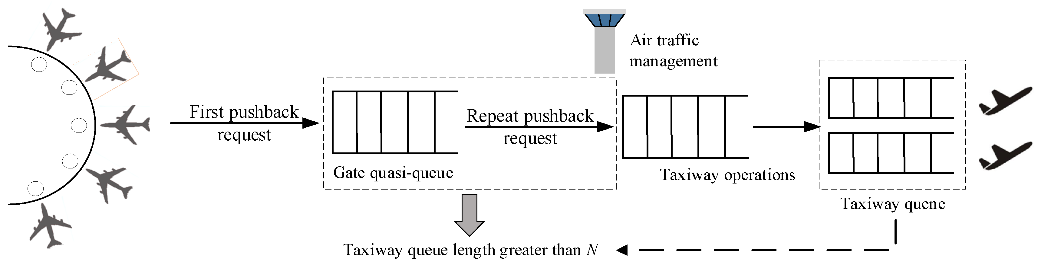
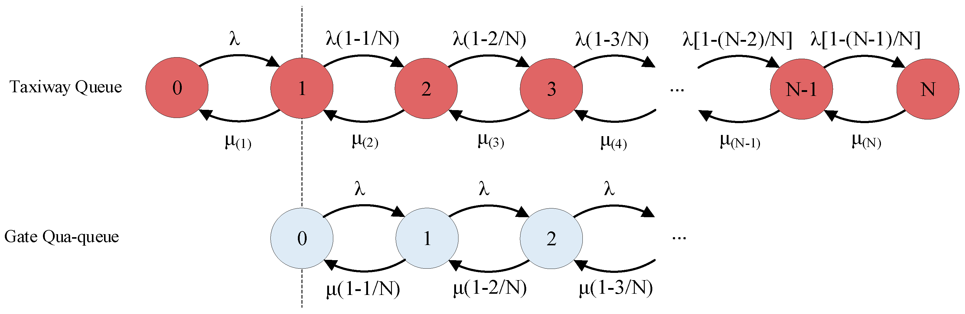
As shown in Figure 2, the multi-runway linear pushback rate control strategy proposed in this paper exhibited a strict Markov property, meaning that pushback permissions are determined by the length of the departure taxiway waiting queue. Moreover, the incorporation of pushback rate control implies that the optimization process for flights should be global, rather than localized to individual flights on the taxiway.

At the gate, flight arrivals follow a Poisson distribution, with an input probability of 1 since the airport cannot reject flight schedules. Consequently, the output rate matches the input rate of the taxiway. For the taxiway, flights enter the overall waiting queue with a probability (1 − n/N), or may be held at the gate with a probability [1 − (1 − n/N)], resulting in gate holding. The service rate μ_(n) is based on the minimum safe distance between consecutive flights. In this study, the wake turbulence separation is adopted as the standard, ensuring that the service rate complies with requirement $\mu (n)={\displaystyle \sum _{r\in R}\mu (n_r)}$ under multi-runway conditions.

For any given queueing state, we assume that:

$$\left[\lambda \left(1-{\displaystyle \frac{n}{N}}\right)+{\mu }_{(n)}\right]{\pi }_{\mathrm{n}}=\lambda \left(1-{\displaystyle \frac{n-1}{N}}\right){\pi }_{n-1}+{\mu }_{(n+1)}{\pi }_{n+1}; n=1,2,\dots ,N-1$$

(20)

where π_n denotes the queue transfer probability, which is not detailed in this paper. In the case of a single runway, typically only the waiting situation at the independent runway gate needs to be considered.

Assuming dual-runway conditions, the service rate should be:

$$\mu (n)=\mu (n_1)+\mu (n_2)={\displaystyle \frac{1}{△t_1(n-1,n)}}+{\displaystyle \frac{1}{△t_2(n-1,n)}}$$

(21)

Building on these characteristics, this paper presents an enhanced threshold iterative optimization algorithm that leverages a CTMC framework. The algorithm systematically searches for the lowest cost across various taxiway queue length thresholds through an iterative process. In stage I, the goal is to determine the optimal taxiway queue threshold N using a fixed service rate. In stage II, the CTMC framework is improved by interactively embedding heuristic algorithms based on fixed queue thresholds and variable service rates. This section emphasizes the application of the first stage, focusing on defining taxiway queue thresholds to ensure broad applicability. To demonstrate the effectiveness of the pushback control strategy, the differences in wake turbulence separation across aircraft types were averaged based on the aircraft type proportions in the example data. The fixed service rate for airports with r runways for stage I at this point should be:

$$\mu (n)={\mu }_{\mathrm{ave}}•r$$

(22)

The pseudo-code is provided in Algorithm A1, and the main steps are as follows:

Step 1: Parameter initialization. Flights are ordered by pushback request times based on the FCFS principle, ensuring that they are processed in chronological order. Key parameters, including the initial queue length for the iterative algorithm, the average wake turbulence separation μ_ave, and taxiway capacity, are also initialized.

Step 2: Taxiway capacity loop. The outer loop for taxiway capacity begins with the capacity determined by the airport’s configuration. The goal of this loop is to continuously update and simulate different taxiway queue length thresholds to find the optimal taxiing conditions, as long as the taxiway capacity does not exceed the configuration limit.

Step 3: Flight sequence loop. For each flight waiting for pushback, the system evaluates the current taxiway queue length n. When the queue length is less than N, the system uses the DPC method to control flight(i). The service rate is set to calculate the taxiway’s queue state at each moment. If the allowable pushback interval is greater than or equal to μ(n) and meets the input requirements, flight(i + 1) is permitted to join the taxiway waiting queue. The interaction between the taxiway capacity and pushback operations is assessed through simulation. If the calculated G_i value exceeds G_max during the evaluation, the inner loop is terminated, and the system proceeds to the outer loop, marking the N value as infeasible.

Step 4: Cost metric calculation. The simulation calculates cost metrics, such as pushback waiting time and taxiway usage, for each pushback request, denoted as C_Tj. The cumulative cost across the entire threshold N, represented as C_TN, forms the basis for selecting the optimal taxiway queue threshold in subsequent steps.

Step 5: Optimization and identification of optimal values. Upon the completion of all outer and inner loops, the calculated C_TN values are compared with the determined optimal taxiway queue length W along with its corresponding taxiway waiting time G and associated parameters. The goal was to identify the queue length threshold that minimized the total system cost across multiple simulations.

4.2. CTMC-Enhanced Whale Optimization Algorithm

In the context of scheduling departing flights at multi-runway airports, the design of optimization algorithms is of great significance in improving the operational efficiency of airports, reducing flight delays, and lowering the operational costs. Unlike traditional static scheduling approaches, the two-stage scheduling proposed in this paper is a coordinated optimization problem characterized by dynamicity and complexity, requiring real-time adjustments to adapt to constantly changing airport ground conditions. Thus, the algorithm needs to be highly adaptable with strong global search capabilities.

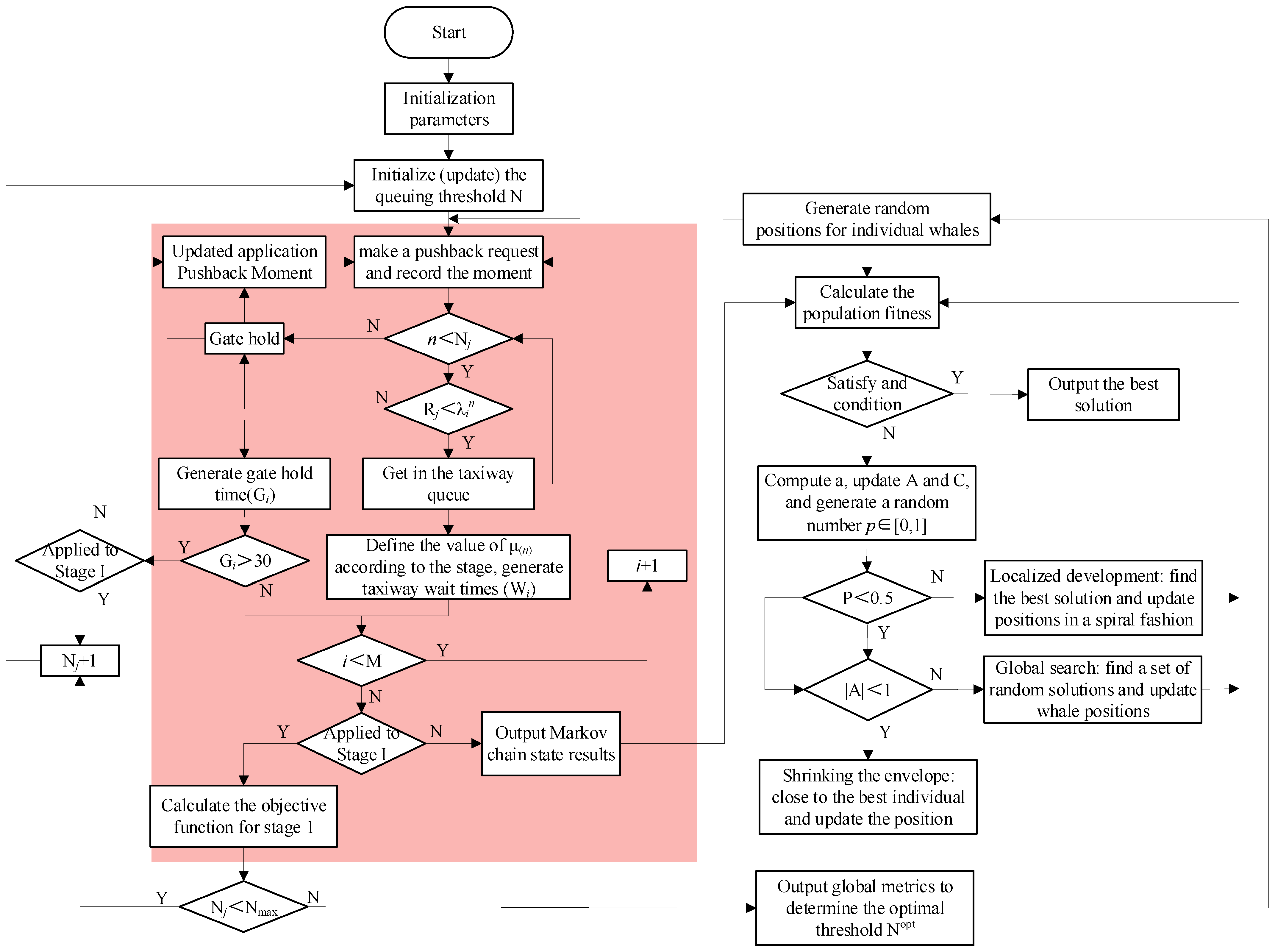
The whale optimization algorithm (WOA) is a swarm intelligence optimization technique inspired by the hunting behavior of humpback whales [29]. It utilizes strategies like encircling prey and spiral updating to explore multiple regions of the solution space, effectively preventing premature convergence and enhancing flexibility and robustness in complex airport environments. Building on this, we proposed integrating the improved CTMC-based algorithm within the WOA, allowing the algorithm to adjust flights in real-time based on current taxiway queue lengths. Specifically, CTMC interactions are embedded within each individual to assess fitness, and under this condition, the optimal solutions for flight sequencing and runway assignment are determined during the scheduling period, thereby adapting to changes in the airport ground conditions. The interaction framework and algorithm flow are illustrated in Figure 3.

The pseudo-code is provided in Algorithm A2, and the main steps are as follows:

Step 1: Population initialization. A population of size K is initialized as X = {X₁, X₂, X₃,⋯X_K}, consisting of multiple individuals, each representing a flight scheduling solution that includes flight sequencing and runway assignment, like X_i = {(f₁, r₁), (f₂, r₂),⋯, (f_n, r_n)}. Each solution, known as a position vector, represents a point in the algorithm’s search space. The initial flight order for all scheduling solutions follows the FCFS rule.

Step 2: Fitness calculation (interaction phase). The overall fitness is calculated from the updated flight states, ensuring that each flight’s status accurately reflects the latest ground conditions. During each fitness evaluation X_i, the CTMC algorithm is run within the scheduling solution to adjust and update the position of each whale individual. This process involves implementing a linear dynamic pushback control strategy within the flight sequence and runway assignment of each individual, enabling state transitions in the Markov chain based on the wake turbulence separation between consecutive flights. The CTMC algorithm further optimizes the individual’s state, with the output rate of the taxiway waiting queue governed by Equation (21). The specific steps are detailed in steps 3 and 4 in the previous section. To account for the interdependence and correlation between the two objectives, the optimization process was made comparable and effective by normalizing both objectives. This approach aimed to reflect the maximum potential values of different objectives, allowing for a comparison on the same scale. Therefore, the objective was set as the minimum total sum of the normalized delay levels and costs.

$$f(X_i)=\left[C_1-\min (C_1)\right]/\left[\max (C_1)-\min (C_1)\right]+\left[C_2-\min (C_2)\right]/\left[\max (C_2)-\min (C_2)\right]$$

(23)

Here, the value of Z ranges from [0, 2], assuming equal importance and weight for the delay levels and departure costs in this study. These weights can be adjusted based on the specific needs of the airport. This setup allows the whale optimization algorithm to not only optimize the scheduling solution, but also adapt dynamically to changes in the airport ground conditions.

Step 3: Iterative update of whale position (exploitation phase). Each individual searches its neighborhood, targeting the global optimum, and updates all positions in the population relative to this global best. By setting |A| < 1, the algorithm favors intensive searches around the current optimal solution. The hunting strategy employed by the whales is determined by a random number p ∈ [0, 1]: if p < 0.5, the encircling prey behavior is chosen, where individuals gradually move closer to the target by adjusting their distance to the optimum; otherwise, the spiral bubble-net attack is selected, with whales approaching the optimum along a spiral path. To emulate both behaviors, it is assumed that the likelihood of whales updating their position via contraction and spiral paths is 0.5 each. The whale’s next position is determined by Equation (24).

$${\overrightarrow{X}}_i(t+1)=\{\begin{array}{ll}{\overrightarrow{X}}_i^{*}(t)-A•\overrightarrow{D}& ifp<0.5\\ \overrightarrow{D}•e^{bl}•\cos (2\pi l)+{\overrightarrow{X}}_i^{*}(t)& ifp\ge 0.5\end{array}$$

(24)

Here, $\overrightarrow{X_i}(t)$ and $\overrightarrow{X_i^{*}}(t)$ represent the candidate solution and the current local optimal solution in iteration t, respectively. B is a constant and l is a random number with the value between −1 and 1. $\overrightarrow{A}$ and $\overrightarrow{C}$ are the coefficient vectors: $\overrightarrow{A}$ is used to control the extent to which the searching whale moves toward or away from the selected target. It simulates the behavior of a whale circling its prey by controlling the exploration and exploitation balance of the solution; the coefficient $\overrightarrow{C}$ is used to determine the path and direction of the whale around the prey, and the algorithm is made to introduce randomness in the updating of the solution’s location and enhance the algorithm’s global search capability by setting $\overrightarrow{C}$ to twice its random value. This is formulated as:

$$\overrightarrow{A}=2•\overrightarrow{r_1}•\overrightarrow{a}-\overrightarrow{a}$$

(25)

$$\overrightarrow{C}=2•\overrightarrow{r_2}$$

(26)

$$\overrightarrow{a}=2-2t/t_{max}$$

(27)

where $\overrightarrow{r_1}$, $\overrightarrow{r_2}$ is a random number in [0, 1], a represents a linearly decreasing value from 2 to 0 based on the ratio of iteration t to the maximum number of iterations t_max. This serves as the distance between the i-th individual and the current global optimal solution in iteration t, as shown below:

$$\overrightarrow{D}=\left\{\begin{array}{ll}\left|\overrightarrow{C}•{\overrightarrow{X}}_i^{*}(t)-{\overrightarrow{X}}_i(t)\right|& ifp<0.5\\ \left|{\overrightarrow{X}}_i^{*}(t)-{\overrightarrow{X}}_i(t)\right|& ifp\ge 0.5\end{array}\right.$$

(28)

Step 4: Random search position (exploration phase). To seek to explore more of the search space, when |A| ≥ 1|, whale individuals perform random searches away from the current optimal solution, forcing candidate solutions to move toward randomly chosen positions. It is assumed that these random solutions are either optimal or near-optimal, prompting a global search.

$$\overrightarrow{X_i}(t+1)={\overrightarrow{X}}_i^{rand}(t)-A•\overrightarrow{D}$$

(29)

The distance value at this stage is defined as:

$$\overrightarrow{D}=\left|\overrightarrow{C}•{\overrightarrow{X}}_i^{rand}(t)-{\overrightarrow{X}}_i(t)\right|$$

(30)

5. Case Study

5.1. Data Sources and Process

This section presents the computed results of the departure process. The datasets used in this study were the Aviation System Performance data (2013) of PEK from the Second Research Institute of Civil Aviation Administration of China, with a huge traffic volume including details on aircraft models and configurations, flight numbers, aircraft categories, origin–destination pairs, scheduled and actual departure times as well as pushback requests. PEK is one of the busiest hub airports in the world, with saturated traffic demand and frequent flight delays. It was recognized as China’s busiest airport and the second busiest globally in 2017 [30]. In September 2024, based on the number of outbound seats, it ranked as the busiest airport in China [31]. Due to data access limitations, a preliminary analysis was conducted using flight data from October to December 2013, chosen for its consistency with flight schedules over six months. This analysis provided the average daily departure demand and delay averages, ensuring the reliability of the study results. As shown in Figure 4, departure demand at PEK increased sharply after 6 a.m., peaked around 8 a.m., and remained high until 9 p.m. The delay patterns exhibited regular fluctuations, showing a leading trend influenced by both inbound and outbound flight demands.

The airport’s runways, from west to east, were designated as 36L/18R, 36R/18L, and 01/19. For the case analysis, departure data from runways 36L/18R and 36R/18L on 1 November 2013, were used including pushback requests for 775 departing flights. Figure 4 shows the hourly departure demand and average flight delay time. Considering variations in taxi distances under different runway and gate combinations, the apron was divided into 33 zones based on the layout of gates and runways at PEK. The zones are shown in Figure 5. As shown in Figure 6, based on the zoning, the unobstructed taxi time from each zone to the south end of the runway was calculated to simplify the scenario optimization process.

To maintain continuous pushback operations, stage I utilizes all-day data, while stage II optimizes the sequencing and assignment for 147 departing flights during the peak period from 9:00 to 10:00, based on an all-day pushback control strategy. Additionally, in compliance with China’s civil aviation development policies, this study adopted the RECAT-CN standards established by the Civil Aviation Administration of China (CAAC) in 2019. These standards, based on both international and domestic experiences, classify aircraft into the Super Heavy (J), Heavy (B), Lower Heavy (C), Medium (M), and Light (L) categories according to the maximum take-off weight and wingspan. Specific values are displayed in

Table 2. RECAT-CN wake turbulence separation standards.

Preceding	Following(s)
	J	B	C	M	L
J	65	110	120	140	159
B	65	60	80	100	140
C	65	65	65	70	120
M	65	65	65	65	100
L	65	65	65	65	65

.

5.2. Result Analysis

Simulations were conducted for both the pushback control and sequencing phases. This study overcame the previous limitation of treating the taxiway queue as a single-server system by implementing a multi-server queue model. Figure 7 shows the simplified results of the taxiway queue lengths for single- and dual-runway configurations without pushback control. Clearly, without considering the complexities of airport operations, a dual-runway setup is more effective than a single runway, significantly reducing the number of flights queued on the taxiway. However, comparing this to the departure demand in Figure 4a revealed that if the peak demand for departing flights persists without scheduling measures, taxiway queues will accumulate due to slow dissipation. This highlights the need to integrate a linear dynamic pushback control model for optimization.

Figure 8 illustrates the cost variation during the pushback control phase as the taxiway queue threshold N changes, aimed at finding the optimal threshold for daily pushback demand. To enhance model adaptability, stage I does not distinguish by aircraft type, setting the service intensity as the average wake turbulence separation based on a mix of aircraft types. Values of N below 5 were omitted due to excessively high costs. The optimal solution for dual-runway scenarios occurred at N = 9, while for single-runway scenarios, it was at N = 13. The corresponding average taxiway queue time and gate-hold time are shown in

Table 3. Metrics for the single-runway and dual-runways configurations at the optimal threshold N.

	Single Runway	Dual Runways
G* (min)	13.59	9.94
W* (min)	16.51	11.58

. Clearly, the higher service intensity of dual runways accelerated the dissipation of taxiway queues, resulting in a lower optimal threshold N, indicating stricter pushback control. Under the optimal threshold, the time metrics for dual runways were more favorable. Additionally, because the gate-hold penalty in the objective function is an exponential term, once the queue threshold exceeds a certain limit, the cost curve shifts from being dominated by the taxiway queue time to being influenced by the gate-hold time. This value represents the point where the average taxiway queue time and gate-hold time are optimized.

For the CTMC-enhanced whale optimization algorithm used in this study, a population size of 50 and 100 iterations were set in stage II. This dynamic scheduling approach can quickly yield reasonable optimization results, showing better optimization capabilities and convergence. The subsequent section will analyze the sequencing and assignment outcomes.

Table 4. Results analysis of the cases.

CASE	1	2	3	4
G* (min)	0.00	0.00	9.94	9.52
W* (min)	23.48	22.63	11.58	10.08
T* (min)	23.48	22.63	24.09	19.60
C1 (s)	18,177.00	17,523.88	18,649.60	17,504.12
C2 (RMB)	349,030.72	338,680.81	292,665.64	279,505.03
CP (RMB)	0.00	0.00	36,616.42	35,646.58
CF (RMB)	225,973.61	216,369.95	165,841.07	157,873.20
CE (RMB)	123,057.11	122,310.86	90,208.15	85,985.25

outlines four scenarios under optimized flight sequencing: (1) no pushback control and no sequencing optimization, (2) no pushback control but with sequencing optimization, (3) pushback control without sequencing optimization, and (4) pushback control with sequencing optimization. It presents the average gate-hold time, average taxiway waiting time, delay deviation, and various cost values for each case. Here, T* represents the total sum of waiting times.

The results show that implementing pushback strategies primarily shifted the taxiway queue time to the gate-hold time, keeping the overall time fluctuations stable. In contrast, scheduling optimization helped to reduce the total waiting times. Comparing CASE 1 and CASE 2 revealed that sequencing optimization without pushback control effectively reduced the flight delays, but due to a lack of control over ground operations, higher taxiway waiting times still resulted in increased costs. A comparison of CASE 1 and CASE 3 illustrated the effectiveness of the proposed linear dynamic pushback control in reducing the taxiway waiting times, which significantly lowered the departure operation costs and enhanced the environmental benefits for the airport. However, it did not substantially improve the flight delay reduction. CASE 4 integrated the optimizations from CASE 2 and CASE 3, representing the final goal of this study. By incorporating delay prioritization based on seat occupancy, both the departure costs and delays were further minimized, with the average flight delay reduced by 4.58 min compared with the non-optimized scenario.

Figure 9 shows a comparison of the pushback phase costs, fuel consumption costs, and environmental costs as well as the average flight waiting time. The results clearly show that pushback control significantly reduced the taxiing fuel consumption, with reductions of about 26.61% and 30.14% in CASE 3 and CASE 4, respectively, compared with CASE 1. In addition, the reason why CASE 3 had a higher value of delay than CASE 1 is that we believe that pushback control focuses on the economic benefit rather than the value of time, when in fact they should be on an equal footing. Thus, the synergistic benefits of combining pushback control with flight sequence optimization to improve the operational efficiency of airports were clearly demonstrated. At the same time, our analysis of each flight involved in the optimization phase revealed that CASE 4 handled outliers better, with superior aggregation with the expected take-off times.

As shown in Figure 10, the departure times during peak periods clearly illustrate the impact of the pushback control strategy. During the pre-peak phase, such as segment A, interactions between taxiway queue time and gate-hold time were evident. Throughout the sustained peak period, the conversion from taxiway queue time to gate-hold time became more prominent, with the gate-hold time taking the lead, effectively reducing on-ground taxiing. This study set a maximum gate-hold time of 30 min, after which flights had to push back. Segment B shows that when consecutive flights remain at the gate for the maximum hold time, the taxiway queue time initially rises and then falls, highlighting the effectiveness of pushback control during peak periods. For instance, the 204th departing flight, where the strategy’s impact was most notable, saw a reduction of 24.47 min in taxiway waiting time using the proposed dynamic scheduling method.

Table 5. Optimized scheduling plan (partial).

No.	Flight Number	Type	Pushback Time	Gate-Hold Time	Taxiway Queue Time	Runway	Delay Reduction Rate
1	HU7245	B	7:41	3	11.59	36R	−6.38%
2	CZ3634	M	7:50	9	4.72	36R	57.66%
3	CA1147	M	7:43	2	13.85	36R	−38.14%
4	MF8192	M	7:47	5	11.98	36R	2.48%
5	CA1461	M	7:45	3	16.11	36R	4.40%
6	CA1877	M	7:42	0	10.04	36L	34.44%
7	HU7103	M	7:45	3	19.14	36R	5.35%
8	CA4125	M	7:54	10	12.27	36R	20.56%
9	CZ3684	M	7:46	0	9.21	36L	22.60%
10	CA1459	M	7:59	12	9.29	36R	35.78%
11	CZ3740	M	7:51	3	19.42	36R	−1.36%
12	SC1198	M	8:05	17	7.55	36R	51.59%
13	HU7115	M	7:50	1	6.86	36L	45.90%
14	CA1509	M	7:57	8	16.89	36R	−5.99%
15	CA1231	M	7:55	6	3.99	36L	73.06%
16	HU7137	M	8:06	17	10.02	36R	44.52%
17	CZ6116	M	7:51	1	10.12	36L	36.51%
18	HU7607	B	8:03	13	15.15	36R	21.07%
19	MU5102	B	7:53	2	10.25	36L	39.95%
20	CA1343	M	8:04	12	17.07	36R	15.14%
AVE	-	-	-	6.35	11.78	-	22.96%

presents a partial schedule of flights under the optimized plan. The delay reduction rate was calculated as the ratio of the difference in departure times between CASE 1 and CASE 4 to the departure time in CASE 1, indicating the degree of optimization for each flight. The optimized scheduling reflects the influence of arriving flights, with a noticeable preference for runway 36R over 36L, underscoring its role as the primary departure runway. By factoring in the distance from the gates to the runway, the method partially achieved multi-gate group pushback, as seen with flights 90/101 and 99/105, thus addressing the limitations of traditional pushback theories in parallel operations. Although not all flights experienced reduced delays, the proposed dynamic scheduling method effectively minimized delays for most flights. Among the selected examples, the average delay reduction rate was 22.96%, with the 15th flight achieving a reduction of up to 73.06%.

6. Summary and Conclusions

To address the complexities of airport ground operations and flight scheduling, this paper introduced a dynamic scheduling method for departing flights, shifting the traditional approach from discrete to continuous optimization. A joint model integrating pushback control and sequencing assignment was developed, with dynamic continuity managed through CTMC nested within a whale optimization algorithm. Case analysis was conducted using historical data from Beijing Capital International Airport, and the main findings were as follows:

• Multi-runway airports were modeled as queuing systems, with CTMC introduced to depict the state transitions of departing flights in taxiway queues. By integrating runway assignments, the service rate for each state was dynamically adjusted, effectively capturing the dynamic behavior of the taxiway queuing system over time.
• Pushback control strategies significantly reduced the taxiway waiting times, yielding cost savings and environmental benefits, consistent with green aviation trends. However, this strategy primarily shifts the individual flights’ taxiway waiting time to gate-hold time under the FCFS principle, balancing resource use without substantially affecting departure delays.
• Sequencing optimization notably reduced the delay levels, and when combined with the linear dynamic pushback control strategy, it improved the overall operational synergy. Compared with non-optimized scenarios, the taxiway waiting times dropped by 55.58%, and the total departure time decreased by 5.86%, alleviating congestion and enhancing on-time performance. This highlights the synergistic benefits of the joint optimization approach in reducing delays and improving scheduling.

The study’s pushback control thresholds were set based on full-day operations to manage sequencing and runway assignment at multi-runway airports, enabling dynamic adjustments to ground traffic changes. Potential future research directions include the following. (1) Refining the time-based mechanism by adjusting the pushback thresholds dynamically in response to fluctuating demand, improving model flexibility and accuracy, and better aligning with real-world airport traffic. (2) In fact, the departure route of the aircraft is also a key factor in runway selection, which requires us to consider specific departure route planning. To validate the methodology, this aspect was not considered in the current study. Based on this, further work is needed to account for variable fuel consumption rates across different taxiing phases to optimize fuel use. (3) The model uses wake turbulence separation as a service time consideration for the pushback control system; however, route separation is also applicable. In the next phase of our work, we will integrate route separation with wake turbulence separation to ensure sufficient airborne separation between aircrafts on similar routes. (4) Exploring the applicability of this scheduling method in other fields requiring multi-entity coordination such as real-time task prioritization in workshop scheduling or adaptive power dispatch in electric grids to respond to load variations.