A Generalized Super-Twisting Extended State Observer for Angle-Constrained Terminal Sliding Mode Guidance Law

Abstract

In this article, a novel finite-time convergent three-dimensional terminal sliding mode guidance law is proposed for intercepting maneuvering targets in three-dimensional space with terminal angle constraints. The proposed guidance law introduces a novel generalized super-twisting extended state observer (GSTESO) to estimate the maneuvering target’s acceleration and lumped disturbances, enabling quicker convergence to the true values and offering better noise tolerance. Moreover, a time-varying function called time base generator (TBG) is introduced in the design of the sliding surface, forming a new terminal sliding mode function that ensures that the line-of-sight (LOS) angle converges within a small neighborhood of the desired value at interception. It also offers good robustness and higher guidance accuracy, effectively avoiding overload saturation in the initial stages of guidance. Simulation results indicate that the proposed TBG-based finite-time terminal sliding mode (TBGFTTSM) guidance law can reduce overload magnitude and ensure continuous and smooth guidance commands, while the performance of the GSTESO is also validated.

1. Introduction

With the increasing threat of maneuvering targets, advanced missile–target interception guidance research based on terminal angle constraints has garnered significant attention [1,2]. Over the past few decades, various methods have been explored to develop guidance laws with termianl angle constraints, including the proportional navigation guidance additional bias term, optimal control theory, sliding mode variable structure control theory [3,4,5], and others. The basic idea of the proportional guidance with additional bias term method [6,7,8] is to introduce extra bias parameters to design guidance laws that satisfy the constraints of miss distance and terminal angle. These guidance laws are not only in a simple form to be easy implemented but also are mainly effective against stationary or slow-moving targets and inadequate for high-speed, highly maneuverable targets [9]. Optimal control methods, which are extensively studied, aim to derive guidance laws with terminal angle constraints by minimizing performance indices. For instance, the study [10] utilized linear quadratic optimal theory to propose a guidance law that incorporates terminal angle constraints to engage maneuvering targets with constant acceleration. Another reference [11] introduced a modeling approach targeting an ideal LOS as the control objective and designed a trajectory-shaping optimal guidance law based on constraints on the terminal relative motion direction and missile overload. While these optimal control methods achieve satisfactory control accuracy, they all require estimation of the time-to-go parameter, which is challenging in practical applications.

Given the short terminal guidance time, it is necessary to design guidance laws that converge within a finite time. As a result, the sliding mode variable structure control theory with finite-time convergence has gained widespread application in the design of guidance laws in recent years. References [12,13,14] employed the terminal sliding mode (TSM) control method to design guidance laws that enable the terminal angle and LOS angle rate to converge to the desired impact angle and zero, respectively, within a finite time. These studies also utilized finite-time control theory to solve for specific convergence times. However, existing TSM and fast terminal sliding mode (FTSM) controllers commonly suffer from a singularity issue when the error approaches zero on the terminal sliding mode surface. To address this issue, the nonsingular terminal sliding mode (NTSM) was proposed, which achieves finite-time convergence and avoids singularity problems, as validated by references [15,16,17,18]. It should be noted that references [16,18] employed a saturation function to replace the sign switching function to eliminate chattering, which introduces steady-state errors. Moreover, these guidance laws are designed for nonmaneuvering targets. For maneuvering targets, references [15,19] proposed guidance laws based on the NTSM but that require estimation of the target’s maneuvering upper limits and still encounter chattering issues. To address these challenges, reference [20] used an adaptive method to estimate the upper bound of target acceleration. However, this method requires a large adaptive switching gain to ensure the robustness of the closed-loop system, which in turn increases energy consumption and induces undesired vibrations. Another approach involves using observers to estimate unknown disturbances, where some scholars apply adaptive techniques to estimate the upper bound of unknown system disturbance and design finite-time-convergent terminal-angle-constrained guidance laws [20,21,22,23]. Nevertheless, ensuring the system’s robustness might necessitate high adaptive gain values, leading to large overload amplitudes and increased energy consumption. An alternative solution is to use observers (typically extended state observers or disturbance observers) to estimate and compensate for unknown target acceleration, thereby designing finite-time-convergent terminal-attack-angle-constrained guidance laws [17,24]. This strategy effectively avoids the need for large adaptive switching gain values.

The convergence time of the aforementioned finite-time guidance law is easily influenced by the initial state of the system and lacks a definite upper bound. This may result in significant errors in the observer during the initial phase, potentially leading to saturated guidance commands. In recent years, many authors have proposed various controllers based on the time base generator (TBG) in different fields [25,26,27,28]. This type of controller has the following characteristics [25,27]: by adjusting the TBG function gain and control parameters, not only can the convergence range of the system state reach ideal values, but the output of the system can also become smoother and more reasonable. Additionally, the system convergence time is not affected by the initial conditions. In references [29,30], the authors proposed two guidance laws with impact angle constraints based on different time-varying functions, but both were assessed within simulated two-dimensional guidance contexts employing a Linear Extended State Observer (LESO) to estimate the unknown system disturbance. The traditional LESO struggles with suppressing time-varying disturbances. Although increasing the LESO’s bandwidth can improve its disturbance rejection capabilities, the bandwidth is constrained by system stiffness. Reference [31] introduced a high-gain ESO as a substitute for the conventional LESO, exploiting its high-gain error attenuation properties to achieve rapid and precise observation of system states and cumulative disturbances, and considering that our guidance system is generally nonlinear, its robustness is not satisfactory. References [32,33,34] designed a nonlinear LESO based on fractional power functions, but they introduced some new parameters to be adjusted and did not carry out simulation analysis on the introduced parameters, so it was not convincing. Therefore, it is necessary to design a faster, more accurate, and more robust observer.

Based on the above considerations, this paper designs a three-dimensional finite-time terminal sliding mode guidance law with terminal angle constraints based on the TBG. Compared to the traditional NSTM guidance laws, our guidance law enables the system to effectively converge to the ideal value in the terminal phase by employing a TBG-function-based terminal sliding mode function. This approach reduces energy consumption and avoids high overloads at the initial phase. Finally, we design a GSTESO that contrasts with the improved ESO in reference [35], which relies solely on nonlinear terms. The proposed GSTESO achieves faster convergence when the estimation error is distant from the equilibrium point and does not depend on the upper bounds of uncertainties. Additionally, compared to the improved ESO discussed in [36], which includes both linear and nonlinear terms, the proposed GSTESO does not introduce any additional parameters that require tuning.

2. Preliminaries and Problem Setup

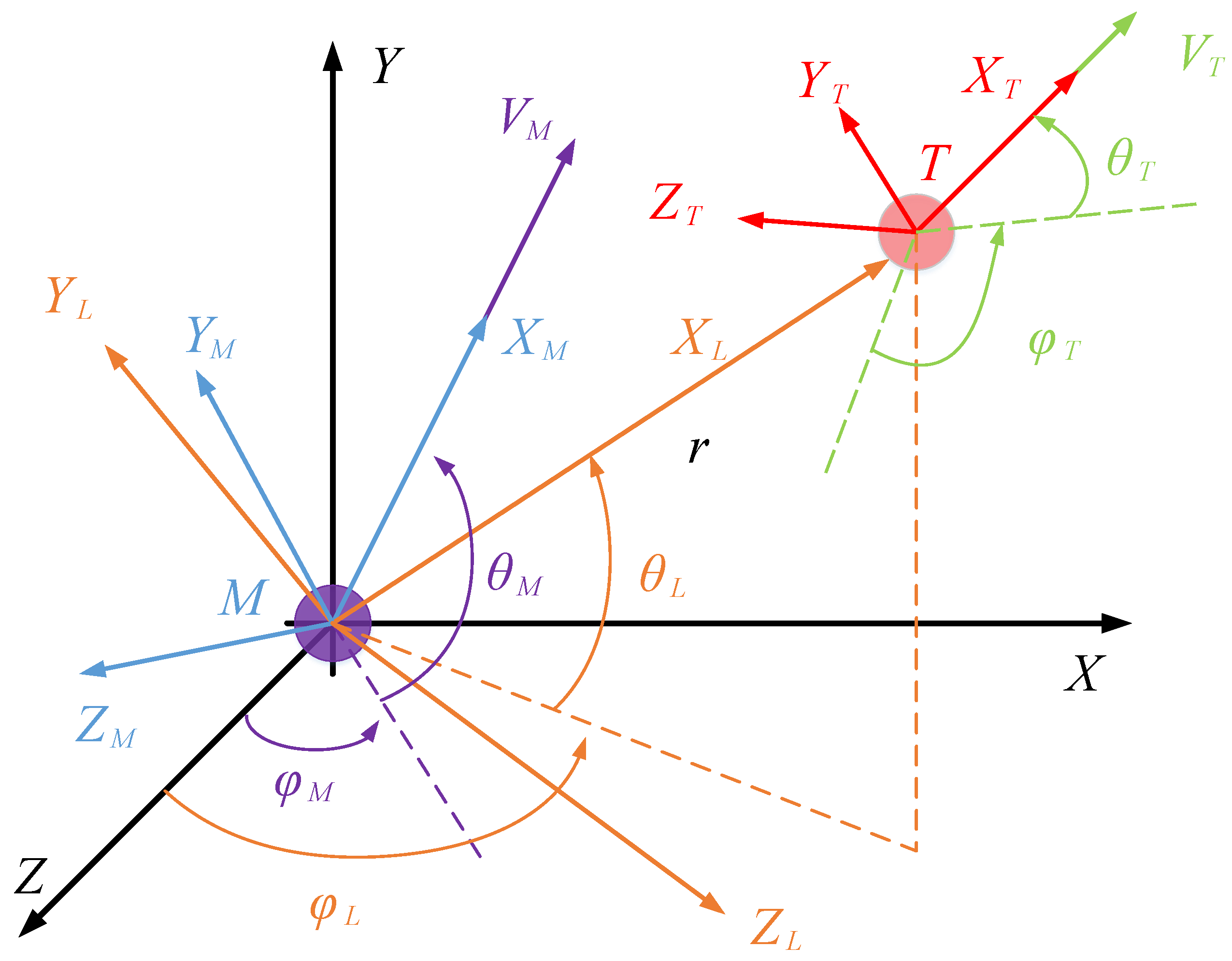
2.1. Relative Kinematics and Problem Formulation

In the segment depicted in Figure 1, the engagement geometry between the target and the missile in 3D is illustrated. $MXYZ$ and $M{X}_L{Y}_L{Z}_L$ represent the inertial coordinate system and the line-of-sight (LOS) coordinate system, respectively. $M{X}_M{Y}_M{Z}_M$ and $T{X}_T{Y}_T{Z}_T$ denote the missile’s and the target’s trajectory coordinate systems, where M and T are the missile and the target respectively, and the target and missile are regarded as constant-velocity point masses. The variables V and $V_T$ stand for the velocities of the missile and the target. $r,{\theta }_L,{\phi }_L$ represent missile–target relative distance, the elevation angle, and two LOS angles in different directions under the inertial reference frames, respectively. ${\theta }_M,{\phi }_M$ and ${\theta }_T,{\phi }_T$ denote the trajectory deviation angle and the LOS angle of the missile and the target, respectively. All angles in Figure 1 are considered positive when measured counterclockwise.

The equations of motion for the missile’s and target’s centers of mass can be represented as follows:

$$\left[\begin{array}{c}{\dot{X}}_M\\ {\dot{Y}}_M\\ {\dot{Z}}_M\\ {\dot{\theta }}_M\\ {\dot{\phi }}_M\end{array}\right]=\left[\begin{array}{c}{V}_{M}cos{\theta }_{M}cos{\phi }_M\\ V_{M}sin{\theta }_M\\ -V_{M}cos{\theta }_{M}sin{\phi }_M\\ a_{My}/V_M\\ -a_{Mz}/V_{M}cos{\theta }_M\end{array}\right]$$

(1)

$$\left[\begin{array}{c}{\dot{X}}_T\\ {\dot{Y}}_T\\ {\dot{Z}}_T\\ {\dot{\theta }}_T\\ {\dot{\phi }}_T\end{array}\right]=\left[\begin{array}{c}{V}_{T}cos{\theta }_{T}cos{\phi }_T\\ V_{T}sin{\theta }_T\\ -V_{T}cos{\theta }_{T}sin{\phi }_T\\ a_{Ty}/V_T\\ -a_{Tz}/V_{T}cos{\theta }_T\end{array}\right]$$

(2)

where $a_{My}$ and $a_{Mz}$ represent the components of the missile’s acceleration vector in the inertial coordinate system, while $a_{Ty}$ and $a_{Tz}$ denote the components of the target’s acceleration vector in the same system. The corresponding relative kinematic equations in the LOS reference frame can be expressed as follows:

$$\ddot{r}-r{\dot{\theta }}_L^2-r{\dot{\phi }}_L^2{cos}^2{\theta }_L=a_{Tr}-a_{Mr}$$

(3)

$$r{\ddot{\theta }}_L+2\dot{r}{\dot{\theta }}_L+r{\dot{\phi }}_L^{2}sin{\theta }_{L}cos{\theta }_L=a_{T\theta }-a_{M\theta }$$

(4)

$$-r{\ddot{\phi }}_{L}cos{\theta }_L-2\dot{r}{\dot{\phi }}_{L}cos{\theta }_L+2r{\dot{\theta }}_L{\dot{\phi }}_{L}sin{\theta }_L=a_{T\phi }-a_{M\phi }$$

(5)

where $(a_{Tr},a_{T\theta },a_{T\phi }),(a_{Mr},a_{M\theta },a_{M\phi })$ define the components of the target’s and missile’s acceleration vectors in the LOS coordinate system, respectively. In the terminal guidance phase, the component of the missile–target relative acceleration along the LOS is minimal, and its impact on the missile miss distance and impact angle error can be considered negligible, so both $a_{Tr}$ and $a_{Mr}$ are 0. According to reference [37], intercepting the target at a desired impact angle can be achieved by controlling the terminal LOS angles. Let the desired terminal LOS angles be ${\theta }_{Lf}$ and ${\phi }_{Lf}$. To further define the state variables ${\mathit{x}}_{\mathbf{1}}={[x_{1\theta },x_{1\phi }]}^{\mathrm{T}}={[\theta -{\theta }_{Lf},\phi -{\phi }_{Lf}]}^{\mathrm{T}},{\mathit{x}}_{\mathbf{2}}={[x_{2\theta },x_{2\phi }]}^{\mathrm{T}}={[\dot{\theta },\dot{\phi }]}^{\mathrm{T}}$, the three-dimensional guidance dynamics model can be expressed as follows:

$$\left\{\begin{array}{c}{\dot{\mathit{x}}}_{\mathbf{1}}={\mathit{x}}_{\mathbf{2}}\hfill \\ {\dot{\mathit{x}}}_{\mathbf{2}}=\mathit{F}-\mathit{B}{\mathit{a}}_{\mathit{T}}+\mathit{B}{\mathit{a}}_{\mathit{M}}\hfill \end{array}\right.$$

(6)

where

$$\mathit{F}=\left[\begin{array}{c}-{\displaystyle \frac{2\dot{r}{\dot{\theta }}_L}{r}}-{\dot{\phi }}_L^{2}cos{\theta }_{L}sin{\theta }_L\\ -{\displaystyle \frac{2\dot{r}{\dot{\phi }}_L}{r}}+2{\dot{\theta }}_L{\dot{\phi }}_{L}tan{\theta }_L\end{array}\right],\mathit{B}=\left[\begin{array}{cc}-{\displaystyle \frac{1}{r}}& 0\\ 0& {\displaystyle \frac{1}{rcos{\theta }_L}}\end{array}\right]$$

$${\mathit{a}}_{\mathit{T}}=\left[\begin{array}{c}{a}_{T\theta }\\ a_{T\phi }\end{array}\right],{\mathit{a}}_{\mathit{M}}=\left[\begin{array}{c}{a}_{M\theta }\\ a_{M\phi }\end{array}\right]$$

2.2. Conventional LESO

Assumption 1.

Owing to its physical limit, the target acceleration components $a_{T\theta },a_{T\phi }$ are bounded and satisfy the following conditions: $\left|a_{T\theta }\right|\le d_{11},\left|a_{T\phi }\right|\le d_{12},\left|{\dot{a}}_{T\theta }\right|\le d_{21}$, and $\left|{\dot{a}}_{T\phi }\right|\le d_{22}$, where $d_{11},d_{12},d_{21}$ and $d_{22}$ are positive constants.

Introducing a new vector $\mathit{Z}={\left[r{\dot{\theta }}_L,r{\dot{\phi }}_{L}cos{\theta }_L\right]}^{\mathrm{T}}$ and differentiating $\mathit{Z}$ with respect to time yields

$$\dot{\mathit{Z}}=\mathit{H}+{\mathit{d}}_{\mathit{T}}$$

(7)

where

$$\mathit{H}=\left[\begin{array}{c}-\dot{r}{\dot{\theta }}_L-r{\dot{\phi }}_L^{2}cos{\theta }_{L}sin{\theta }_L-a_{M\theta }\\ -\dot{r}{\dot{\phi }}_{L}cos{\theta }_L+r{\dot{\theta }}_L{\dot{\phi }}_{L}sin{\theta }_L+a_{M\phi }\end{array}\right],{\mathit{d}}_{\mathit{T}}=\left[\begin{array}{c}{a}_{T\theta }\\ -a_{T\phi }\end{array}\right]$$

By considering $d_T$ as a new extended state, the augmented system can be represented as follows:

$$\left\{\begin{array}{c}\dot{\mathit{Z}}=\mathit{H}+{\mathit{d}}_{\mathit{T}}\hfill \\ {\dot{\mathit{A}}}_{\mathit{T}}=\mathit{L}\hfill \end{array}\right.$$

(8)

For the system (8), the conventional LESO can be constructed as

$$\left\{\begin{array}{c}\dot{\widehat{\mathit{Z}}}=\mathit{H}+k_1\left(\widehat{\mathit{Z}}-\mathit{Z}\right)+{\widehat{\mathit{d}}}_{\mathit{T}}\hfill \\ {\dot{\widehat{\mathit{d}}}}_{\mathit{T}}=k_2(\widehat{\mathit{Z}}-\mathit{Z})\hfill \end{array}\right.$$

(9)

where $\widehat{\mathit{Z}}$ and ${\widehat{\mathit{d}}}_{\mathit{T}}$ represent the estimated values of $\mathit{Z}$ and the total disturbance ${\mathit{d}}_{\mathit{T}}$, respectively. The parameters $k_1$ and $k_2$ are components of the LESO and can be chosen as follows:

$$\left\{\begin{array}{c}{k}_1=2\omega \hfill \\ k_2={\omega }^2\hfill \end{array}\right.$$

(10)

where $\omega$ represents the bandwidth of the LESO. Let ${\mathit{e}}_{\mathbf{1}}=\widehat{\mathit{Z}}-\mathit{Z},{\mathit{e}}_{\mathbf{2}}={\widehat{\mathit{d}}}_{\mathit{T}}-{\mathit{d}}_{\mathit{T}}$ and $\mathit{e}={\left[{\mathit{e}}_{\mathbf{1}},{\mathit{e}}_{\mathbf{2}}\right]}^{\mathrm{T}}$; then, the error estimation system can then be obtained as follows:

$$\dot{\mathit{e}}=\mathit{Ae}-\mathit{D}{\dot{\mathit{d}}}_{\mathit{T}}$$

(11)

where

$$\mathit{A}=\left[\begin{array}{cc}{k}_1& 1\\ k_2& 0\end{array}\right],\mathit{D}=\left[\begin{array}{c}0\\ 1\end{array}\right]$$

(12)

Based on reference [38], it is sufficient to ensure that $\mathit{A}$ is a Hurwitz matrix by appropriately selecting the parameters $k_i,i=\left\{1,2\right\}$. The estimation error can then be derived:

$$∥\mathit{e}\left(t\right)∥\le ∥{\mathit{e}}^{\mathit{A}t}∥∥\mathit{e}\left(0\right)∥-∥{\mathit{A}}^{-1}(\mathrm{I}-{\mathit{e}}^{\mathit{A}t})\mathit{D}∥\epsilon$$

(13)

Remark 1.

Based on this premise, it can be deduced that the conventional LESO inevitably introduces steady-state estimation errors, which results in its inaccurate observation of rapidly varying disturbances. Therefore, it is crucial to employ a more robust and precise observer to effectively mitigate time-varying disturbances in the guidance system.

3. Guidance Law Design with Terminal Angle Constraint

3.1. Generalized Super-Twisting Extended State Observer Design

In order to improve the disturbance rejection ability of the guidance system, this section introduces a new GSTESO. The newly proposed GSTESO is formulated as follows:

$$\left\{\begin{array}{c}\dot{\widehat{\mathit{Z}}}={\widehat{\mathit{d}}}_{\mathit{T}}+\mathit{H}+k_1{\mathit{\zeta }}_{\mathbf{1}}\left({\mathit{e}}_{\mathbf{1}}\right)\hfill \\ {\dot{\widehat{\mathit{d}}}}_{\mathit{T}}=k_2{\mathit{\zeta }}_{\mathbf{2}}\left({\mathit{e}}_{\mathbf{2}}\right)\hfill \end{array}\right.$$

(14)

and the nonlinear functions are designed as

$$\left\{\begin{array}{c}{\mathit{\zeta }}_{\mathbf{1}}\left({\mathit{e}}_{\mathbf{1}}\right)={⌊{\mathit{e}}_{\mathbf{1}}⌉}^{{\displaystyle \frac{1}{2}}}+{\mathit{e}}_{\mathbf{1}}\hfill \\ {\mathit{\zeta }}_{\mathbf{2}}\left({\mathit{e}}_{\mathbf{1}}\right)={\displaystyle \frac{3}{2}}{⌊{\mathit{e}}_{\mathbf{1}}⌉}^{{\displaystyle \frac{1}{2}}}+{\displaystyle \frac{1}{2}}·sign\left({\mathit{e}}_{\mathbf{1}}\right)+{\mathit{e}}_{\mathbf{1}}\hfill \end{array}\right.$$

(15)

where the symbol ${⌊·⌉}^x$ is defined as ${\left|·\right|}^x·\mathrm{sgn}(·)$. The parameters for the GSTESO can be set as $k_1=2\omega$ and $k_2={\omega }^2$.

Similarly, the error of system can be expressed as follows:

$$\left\{\begin{array}{c}{\dot{\mathit{e}}}_{\mathbf{1}}=k_1{\mathit{\zeta }}_{\mathbf{1}}\left({\mathit{e}}_{\mathbf{1}}\right)+{\mathit{e}}_{\mathbf{2}}\hfill \\ {\dot{\mathit{e}}}_2=k_2{\mathit{\zeta }}_{\mathbf{2}}\left({\mathit{e}}_{\mathbf{1}}\right)-\dot{\mathit{d}}\left(\mathit{t}\right)\hfill \end{array}\right.$$

(16)

Next, we will verify the stability of the GSTESO. Firstly, let us introduce a new state vector as follows:

$${\mathit{\eta }}^{\mathbf{T}}=[\mathit{\zeta }\left({\mathit{e}}_{\mathbf{1}}\right),{\mathit{e}}_{\mathbf{2}}]$$

(17)

The Lyapunov function is formulated as follows:

$${\mathit{V}}_{\mathbf{1}}={\mathit{\eta }}^{\mathrm{T}}\mathit{P}\mathit{\eta }$$

(18)

where P is a symmetric positive-definite matrix, and the derivative of $\eta$ is given by

$$\begin{array}{c}\dot{\mathit{\eta }}=\mathit{\mu }\left({\mathit{e}}_{\mathbf{1}}\right)\left[\begin{array}{c}{k}_1{\mathit{\zeta }}_{\mathbf{1}}\left({\mathit{e}}_{\mathbf{1}}\right)+{\mathit{e}}_{\mathbf{2}}\\ k_2{\mathit{\zeta }}_{\mathbf{2}}\left({\mathit{e}}_{\mathbf{1}}\right)-\dot{\mathit{d}}\left(\mathit{t}\right)/\omega \left({\mathit{e}}_{\mathbf{1}}\right)\end{array}\right]\hfill \\ =\mathit{\mu }\left({\mathit{e}}_{\mathbf{1}}\right)(\mathit{A}\mathit{\eta }-\mathit{B}\mathbf{\Lambda })\hfill \end{array}$$

(19)

where $\mu \left({\mathit{e}}_{\mathbf{1}}\right)=0.5|{\mathit{e}}_{\mathbf{1}}{|}^{-0.5}+1$, $\mathbf{\Lambda }=\dot{\mathit{d}}\left(\mathit{t}\right)/\mathit{\zeta }\left({\mathit{e}}_{\mathbf{1}}\right)$.

Drawing inspiration from [25], define $\mathbf{\Delta }(\mathit{\zeta },\mathbf{\Lambda })={\left[\begin{array}{c}\mathit{\eta }\\ \mathbf{\Lambda }\end{array}\right]}^{\mathit{T}}\left[\begin{array}{cc}\mathit{C}& \mathit{D}\\ \mathit{D}& -\mathit{\theta }\end{array}\right]\left[\begin{array}{c}\mathit{\eta }\\ \mathbf{\Lambda }\end{array}\right]$, where $\theta \ge 0$; then, by choosing proper matrices $\mathit{C}$ and $\mathit{D}$, it can be ensured that $\mathbf{\Delta }(\mathit{\zeta },\mathbf{\Lambda })\ge 0$.

Theorem 1 [25]: Assume there exists a symmetric positive-definite matrix $\mathit{P}$, along with positive constants $\kappa$ and $\theta$, that fulfill the following matrix inequality:

$$\left[\begin{array}{cc}{\mathit{A}}^{\mathit{T}}\mathit{P}+\mathit{PA}+\kappa \mathit{P}+\mathit{C}& \mathit{PB}+{\mathit{D}}^{\mathit{T}}\\ {\mathit{B}}^{\mathit{T}}\mathit{P}+\mathit{D}& -\theta \end{array}\right]\le 0$$

(20)

System (16) is finite-time stable.

$$\begin{array}{cc}\hfill {\dot{\mathit{V}}}_1& =\mu \left({\mathit{e}}_{\mathbf{1}}\right)\left[{\mathit{\eta }}^{\mathbf{T}}({\mathit{A}}^{\mathit{T}}\mathit{P}+\mathit{PA})\mathit{\eta }+\mathbf{\Lambda }{\mathit{B}}^{\mathit{T}}\mathit{P}\mathit{\eta }+{\mathit{\eta }}^{\mathit{T}}\mathit{PB}\mathbf{\Lambda }\right]\hfill \\ \hfill & =\mu \left({\mathit{e}}_{\mathbf{1}}\right){\left[\begin{array}{c}\mathit{\eta }\\ \mathbf{\Lambda }\end{array}\right]}^T\left[\begin{array}{cc}{\mathit{A}}^{\mathit{T}}\mathit{Q}+\mathit{QA}& \mathit{QB}\\ {\mathit{B}}^{\mathit{T}}\mathit{Q}& 0\end{array}\right]\left[\begin{array}{c}\mathit{\eta }\\ \mathbf{\Lambda }\end{array}\right]\hfill \\ \hfill & \le \mu \left({\mathit{e}}_{\mathbf{1}}\right)\left\{{\left[\begin{array}{c}\mathit{\eta }\\ \mathbf{\Lambda }\end{array}\right]}^T\left[\begin{array}{cc}{\mathit{A}}^{\mathit{T}}\mathit{Q}+\mathit{QA}& \mathit{QB}\\ {\mathit{B}}^{\mathit{T}}\mathit{Q}& 0\end{array}\right]\left[\begin{array}{c}\mathit{\eta }\\ \mathbf{\Lambda }\end{array}\right]+\mathbf{\Delta }(\mathit{\eta },\mathbf{\Lambda })\right\}\hfill \\ \hfill & \le \mu \left({\mathit{e}}_{\mathbf{1}}\right){\left[\begin{array}{c}\mathit{\eta }\\ \mathbf{\Lambda }\end{array}\right]}^T\left[\begin{array}{cc}-\kappa \mathit{P}& 0\\ 0& 0\end{array}\right]\left[\begin{array}{c}\mathit{\eta }\\ \mathbf{\Lambda }\end{array}\right]\hfill \\ \hfill & =-{\displaystyle \frac{\kappa }{2{\left|{\mathit{e}}_{\mathbf{1}}\right|}^{1/2}}}\mathit{V}-\kappa \mathit{V}\hfill \end{array}$$

(21)

According to Equation (18), we can obtain the final result as follows:

$${\psi }_{min}\left\{\mathit{P}\right\}{∥\mathit{\eta }∥}^2\le {\mathit{V}}_{\mathbf{1}}={\mathit{\eta }}^{\mathit{T}}\mathit{P}\mathit{\eta }\le {\psi }_{max}\left\{\mathit{P}\right\}{∥\mathit{P}∥}^2$$

(22)

where $\psi \left\{\mathit{P}\right\}$ represents the eigenvalue of matrix $\mathit{P}$, and ${∥\mathit{\eta }∥}^2=\left|{\mathit{e}}_{\mathbf{1}}\right|+2{\left|{\mathit{e}}_{\mathbf{1}}\right|}^{(3/2)}+{{\mathit{e}}_{\mathbf{1}}}^2+{{\mathit{e}}_{\mathbf{2}}}^2$.

Therefore, ${\left|{\mathit{e}}_{\mathbf{1}}\right|}^{(1/2)}\le \left({{\mathit{V}}_{\mathbf{1}}}^{(1/2)}\right)/\left({\psi }_{min}^{(1/2)}\left\{\mathit{P}\right\}\right)$ holds, and Equation (21) can be rewritten as

$${\dot{\mathit{V}}}_{\mathbf{1}}\le -{\displaystyle \frac{\kappa {\mathit{\psi }}_{min}^{1/2}\left\{\mathit{P}\right\}}{2}}{\mathit{V}}^{1/2}-\kappa \mathit{V}$$

(23)

According to the finite-time stability proof detailed in [32], the error system (16) attains finite-time stability.

3.2. Finite-Time Terminal Sliding Mode Guidance Law Design

First, we provide the following basic concepts and lemmas about the TBG, which will assist in the subsequent stability proof.

The TBG is a time-dependent function that satisfies specific constraints on the initial and final values of the first-order time derivative of the function itself. Consider the following first-order dynamic model.

$$\dot{y}\left(t\right)=u\left(t\right)+d\left(t\right)$$

(24)

where $y\left(t\right)$ represents the system state, $d\left(t\right)$ denotes the lumped uncertainty, which is bounded, and $u\left(t\right)$ signifies the control input, which is expressed as follows:

$$u\left(t\right)=({\displaystyle \frac{m\dot{\beta }\left(t\right)}{\beta \left(t\right)+\delta }}-{\displaystyle \frac{\kappa }{{\left(\beta \right(t)+\delta )}^n}})y\left(t\right)$$

(25)

where $\kappa >0,m\ge n>0,\delta >0$. The TBG function possesses the following general characteristics [25]:

(1)

$\beta \left(t\right)$ is a class $C^l$ function, where $l\ge 2$.

(2)

The function $\beta \left(t\right)$ is non-negative and nonincreasing, with its initial value significantly greater than $\delta$, which is denoted as $\beta \left(0\right)\gg \delta$. Furthermore, it satisfies the condition $\beta \left(t_s\right)=0$ at a predetermined time $t_s$, which represents the specified time constant.

(3)

If $0\le t<t_s$, $\beta \left(t\right)>0$, $\dot{\beta }\left(t\right)$ is bounded, and $\dot{\beta }\left(t_s\right)=0$.

(4)

If $t>t_s$, $\beta \left(t\right)=0$, and $\dot{\beta }\left(t\right)=0$.

Lemma 1.

Consider system (24). If the uncertainty $d\left(t\right)$ satisfies $\left|d\left(t\right)\right|\le \tau$, where τ is an unknown constant, and if the control law is formulated as shown in Equation (25), then the system state $y\left(t\right)$ will converge to the specified region within the given time $t_s$:

$${\Omega }_y=\left\{y\left(t\right)\left|\left|y\left(t_s\right)\right|\le max\left\{{\displaystyle \frac{\tau {\delta }^n}{\kappa }},\left|y\left(0\right)\right|{\left({\displaystyle \frac{\tau }{\beta \left(0\right)+\delta }}\right)}^m\right\}\right.\right\}$$

(26)

Stability Proof: Select the Lyapunov function as follows:

$$V_y={\displaystyle \frac{1}{2}}{y}^2\left(t\right)$$

(27)

Taking the derivative of the above equation with respect to time, we obtain the following:

$$\begin{array}{cc}\hfill {\dot{V}}_y& =y\left(t\right)\dot{y}\left(t\right)\hfill \\ \hfill & \le {\displaystyle \frac{2m\dot{\beta }\left(t\right)}{\beta \left(t\right)+\delta }}{V}_y-{\displaystyle \frac{\kappa }{{\left(\beta \right(t)+\delta )}^n}}{y}^2\left(t\right)+\tau \left|y\left(t\right)\right|\hfill \\ \hfill & \le {\displaystyle \frac{2m\dot{\beta }\left(t\right)}{\beta \left(t\right)+\delta }}{V}_y-{\displaystyle \frac{\kappa y^2\left(t\right)}{2{\left(\beta \right(t)+\delta )}^n}}+{\displaystyle \frac{{\left(\beta \right(t)+\delta )}^n{\tau }^2}{2\kappa }}\hfill \end{array}$$

(28)

For the above equation, the analysis is conducted under the following cases:

If $\left|y\left(t\right)\right|>\tau {\kappa }^{-1}{(\beta \left(t\right)+\delta )}^n$ holds continuously for $0\le t<t_s$, then we can obtain that

$${\dot{V}}_y<{\displaystyle \frac{2m\dot{\beta }\left(t\right)}{\beta \left(t\right)+\delta }}{V}_y,0\le t\le t_s$$

(29)

and according to the comparison principle, we derive the following:

$$\left|y\left(t\right)\right|=\sqrt{2V_y}<y\left(0\right){\left({\displaystyle \frac{\beta \left(t\right)+\delta }{\beta \left(0\right)+\delta }}\right)}^m$$

(30)

From the above equation, it can be concluded that $y\left(t\right)$ will converge to the specified region within the predetermined time $t_s$:

$$\left|y\left(t_s\right)\right|<y\left(0\right){\left({\displaystyle \frac{\delta }{\beta \left(0\right)+\delta }}\right)}^m$$

(31)

If there exists a time constant $0<t_0<t_s$ such that $\left|y\left(t_0\right)\right|\le \tau {\kappa }^{-1}{(\beta \left(t\right)+\delta )}^n$, the system state may exhibit the following two scenarios: If $\left|y\left(t\right)\right|\le \tau {\kappa }^{-1}{(\beta \left(t\right)+\delta )}^n$ holds for all $t_0\le t\le t_s$, we can conclude that the function $y\left(t\right)$ satisfies $\left|y\left(t_s\right)\right|\le \tau {\kappa }^{-1}{\delta }^n$ at the predetermined time $t_s$. If there exist two time constants $t_0<t_1<t_2<t_s$ such that $\left|y\left(t_1\right)\right|=\tau {\kappa }^{-1}{(\beta \left(t_1\right)+\delta )}^n$, and for $t_1<t<t_2$, $\left|y\left(t\right)\right|>\tau {\kappa }^{-1}{(\beta \left(t\right)+\delta )}^n$, then from Equation (28), we can obtain

$${\dot{V}}_y<{\displaystyle \frac{2m\dot{\beta }\left(t\right)}{\beta \left(t\right)+\delta }}{V}_y,t_1\le t\le t_2$$

(32)

and according to the comparison principle, we derive the following:

$$\begin{array}{cc}\hfill \left|y\left(t\right)\right|& =\sqrt{2V_y}<{\displaystyle \frac{y\left(t_1\right){\left(\beta \right(t)+\delta )}^m}{{(\beta \left(t_1\right)+\delta )}^m}}\hfill \\ \hfill & ={\displaystyle \frac{\tau {\kappa }^{-1}{\left(\beta \right(t)+\delta )}^n{\left(\beta \right(t)+\delta )}^{m-n}}{{(\beta \left(t_1\right)+\delta )}^{m-n}}}\hfill \\ \hfill & \le \tau {\kappa }^{-1}{\left(\beta \right(t)+\delta )}^n,t_1\le t\le t_2\hfill \end{array}$$

(33)

This contradicts the assumption that $\left|y\left(t\right)\right|>\tau {\kappa }^{-1}{(\beta \left(t\right)+\delta )}^n$ when $t_1\le t\le t_2$. Therefore, once $y\left(t\right)$ converges to the region $\left\{y\left(t\right)\left|\left|y\left(t\right)\right|\le {\displaystyle \frac{\tau {\left(\beta \right(t)+\delta )}^n}{\kappa }}\right.\right\}$, it will remain in this region and not depart from it. Based on the above analysis, the system state $y\left(t\right)$ will converge to region ${\Omega }_y$ within the predetermined time $t_s$.

Let $\psi \left(t\right)=\left|y\left(t\right)\right|$. Based on Equations (24) and (25), we obtain the following:

$$\dot{\psi }\left(t\right)\le -{\displaystyle \frac{\kappa \psi \left(t\right)}{{\delta }^n}}+\tau ,t>t_s$$

(34)

and according to the comparison principle, we derive the following:

$$\begin{array}{c}\hfill \psi \left(t\right)\le {\displaystyle \frac{\psi \left(t_s\right)}{e^{\kappa (t-t_s)/{\delta }^n}}}+\tau {\delta }^n{\kappa }^{-1}(1-e^{-\kappa (t-t_s)/{\delta }^n}),t>t_s\end{array}$$

(35)

For Equation (35), the analysis is conducted under the following cases:

(1)

When $\left|y\left(t_s\right)\right|\le \tau {\kappa }^{-1}{\delta }^n$, we can obtain the following:

$$\psi \left(t\right)\le \tau {\kappa }^{-1}{\delta }^n{e}^{-\kappa (t-t_s)/{\delta }^n}+\tau {\kappa }^{-1}{\delta }^n(1-e^{-\kappa (t-t_s)/{\delta }^n})={\displaystyle \frac{\tau {\delta }^n}{\kappa }},t>t_s$$

(36)

(2)

When $\tau {\delta }^n/\kappa <\left|y\left(t_s\right)\right|\le y\left(0\right){\delta }^m/{(\beta \left(0\right)+\delta )}^m$, we can obtain the following:

$$\psi \left(t\right)\le \psi \left(t\right)e^{-\kappa (t-t_s)/{\delta }^n}+\psi \left(t\right)(1-e^{-\kappa (t-t_s)/{\delta }^n})=\psi \left(t\right),t>t_s$$

(37)

By integrating Equations (36) and (37), we can conclude that when $t>t_s$, the system state $y\left(t\right)$ consistently remains within region ${\Omega }_y$. This completes the proof of Lemma 1.

Since the goal of this section is to ensure that the LOS angle error $x_1$ and the tangential relative acceleration Z between the missile and target converge to 0 by the end of the interception, and the predetermined time can be set equal to the interception time, i.e., $t_s=t_f$. The TBG time-varying function $\beta \left(t\right)$ can be selected as $\beta \left(t\right)=r-r_f$, with $r_f\le r\left(0\right)$, allowing for the choice $\delta =r_f$. Based on Lemma 1, the TBG-based terminal sliding surface can be constructed as follows:

$$\mathit{s}={\left[s_{\theta },s_{\phi }\right]}^{\mathrm{T}}={\mathit{x}}_{\mathbf{2}}-{\displaystyle \frac{m\dot{r}}{r}}{\mathit{x}}_{\mathbf{1}}+{\displaystyle \frac{\kappa }{r}}{\mathit{x}}_{\mathbf{1}}$$

(38)

where $m>1$; then, differentiate the expression with respect to time.

$$\dot{\mathit{s}}=\mathit{F}+\left({\displaystyle \frac{m{\dot{r}}^2-\kappa \dot{r}}{r^2}}\right){\mathit{x}}_{\mathbf{1}}+\left({\displaystyle \frac{\kappa -m\dot{r}}{r}}\right){\mathit{x}}_{\mathbf{2}}+{\displaystyle \frac{{\mathit{d}}_{\mathit{T}}}{r}}-{\displaystyle \frac{m\ddot{r}}{r}}{\mathit{x}}_{\mathbf{1}}+\mathit{B}{\mathit{a}}_{\mathit{M}}$$

(39)

According to the above equation, the guidance law is designed as follows:

$$\begin{array}{c}{\mathit{a}}_{\mathit{M}}=-{\displaystyle \frac{{\mathit{B}}^{-\mathbf{1}}}{r}}\left(\mathit{F}r+\left({\displaystyle \frac{m\dot{r}-\kappa \dot{r}}{r^2}}\right){\mathit{x}}_{\mathbf{1}}+\left(\kappa -m\dot{r}\right){\mathit{x}}_{\mathbf{2}}+{\widehat{\mathit{d}}}_{\mathit{T}}-\alpha \dot{r}\mathit{s}+c{\mathit{\zeta }}_{\mathbf{3}}\right)\hfill \\ {\mathit{\zeta }}_{\mathbf{3}}=\left|{\mathit{x}}_{\mathbf{1}}\right|\mathrm{sign}\left(\mathit{s}\right)+\mathrm{sign}\left(\mathit{s}\right)\hfill \end{array}$$

(40)

where ${\widehat{\mathit{d}}}_{\mathit{T}}$ is the value estimated by the GSTESO mentioned earlier, while $\alpha$ and c are designed parameters; $\alpha >0,c>max\left\{\alpha \left|\ddot{r}\right|,{∥{\mathit{e}}_{\mathbf{2}}∥}_{\infty }\right\}$.

3.3. Stability Analysis

This section will conduct a stability analysis based on the sliding variable s and LOS angle error ${\mathit{x}}_{\mathbf{1}}$:

(1)

Choose the following Lyapunov function:

$${\mathit{V}}_{\mathbf{2}}=\left[\begin{array}{c}{v}_{\theta }\\ v_{\phi }\end{array}\right]={\displaystyle \frac{\mathit{s}\odot \mathit{s}}{2}}$$

(41)

Then, differentiate the above expression with respect to time:

$$\begin{array}{cc}\hfill {\dot{\mathit{V}}}_{\mathbf{2}}& =\mathit{s}\odot \dot{\mathit{s}}\hfill \\ \hfill & ={\displaystyle \frac{\alpha \dot{r}}{r}}\mathit{s}\odot \mathit{s}-{\displaystyle \frac{1}{r}}\mathit{s}\odot {\mathit{e}}_{\mathbf{2}}-{\displaystyle \frac{m}{r}}\ddot{r}\mathit{s}\odot {\mathit{x}}_{\mathbf{1}}-{\displaystyle \frac{c}{r}}\left|\mathit{s}\right|\odot \left|{\mathit{x}}_{\mathbf{1}}\right|-{\displaystyle \frac{c}{r}}\left|\mathit{s}\right|\hfill \\ \hfill & \le {\displaystyle \frac{\alpha \dot{r}}{r}}\mathit{s}\odot \mathit{s}+{\displaystyle \frac{\left|\mathit{s}\right|}{r}}\odot \left({\mathit{e}}_{\mathbf{2}}-\left[\begin{array}{c}c\\ c\end{array}\right]\right)+{\displaystyle \frac{\left|\mathit{s}\right|\odot \left|{\mathit{x}}_{\mathbf{1}}\right|}{r}}\left(m\ddot{r}-c\right)\hfill \end{array}$$

(42)

where ⊙ is the Hadamard product [39,40] that denotes the multiplication of elements at corresponding positions, for example, $[a,b]\odot [c,d]=[ac,bd]$. Since $c>max\left\{\alpha \left|\ddot{r}\right|,{∥{\mathit{e}}_{\mathbf{2}}∥}_{\infty }\right\}$, the above expression can be rewritten as

$${\dot{\mathit{V}}}_{\mathbf{2}}\le {\displaystyle \frac{\alpha \dot{r}}{r}}\mathit{s}\odot \mathit{s}={\displaystyle \frac{2\alpha \dot{r}}{r}}{\mathit{V}}_{\mathbf{2}}$$

(43)

Suppose the existence of a positive variable x that satisfies $\mathit{X}\left(\mathbf{0}\right)={\left[x\left(0\right),x\left(0\right)\right]}^{\mathrm{T}}={\mathit{V}}_2\left(0\right)$ and $\dot{x}=2\alpha \dot{r}W/r$; we can solve this first-order linear differential equation to obtain the following:

$${\displaystyle \frac{x}{x\left(0\right)}}={\left({\displaystyle \frac{r}{r\left(0\right)}}\right)}^{2\alpha }$$

(44)

Furthermore, we obtain the following:

$${\mathit{V}}_{\mathbf{2}}\le \mathit{X}=\mathit{X}\left(0\right){\left({\displaystyle \frac{r}{r\left(0\right)}}\right)}^{2\alpha }={\mathit{V}}_{\mathbf{2}}\left(0\right){\left({\displaystyle \frac{r}{r\left(0\right)}}\right)}^{2\alpha }$$

(45)

where $\mathit{X}={\left[x,x\right]}^{\mathrm{T}}$. Therefore, according to Equations (41) and (45), the sliding variable satisfies the following:

$$\left|\mathit{s}\right|=\sqrt{2}\left[\begin{array}{c}\sqrt{v_{\theta }}\\ \sqrt{v_{\phi }}\end{array}\right]={\displaystyle \frac{\sqrt{2}}{\sqrt{2}}}\left[\begin{array}{c}\sqrt{s_{\theta }^2}\\ \sqrt{s_{\phi }^2}\end{array}\right]\le \left[\begin{array}{c}\sqrt{s_{\theta }^2}\\ \sqrt{s_{\phi }^2}\end{array}\right]{\left({\displaystyle \frac{r}{r\left(0\right)}}\right)}^{\alpha }=\left|\mathit{s}\right|{\left({\displaystyle \frac{r}{r\left(0\right)}}\right)}^{\alpha }$$

(46)

From the above expression, we can be obtain that the sliding variable will converge to the following region at the time of interception:

$${\Omega }_{\mathit{s}}=\left\{\mathit{s}\left|\left|\mathit{s}\right|\le \left|\mathit{s}\left(\mathbf{0}\right)\right|\right.{\left({\displaystyle \frac{r_f}{r\left(0\right)}}\right)}^{\alpha }\right\}$$

(47)

(2)

Choose another Lyapunov function:

$${\mathit{V}}_{\mathbf{3}}={\displaystyle \frac{{\mathit{x}}_{\mathbf{1}}\odot {\mathit{x}}_{\mathbf{1}}}{2}}$$

(48)

Similarly, differentiating the above equation with respect to time yields the following:

$$\begin{array}{cc}\hfill {\dot{\mathit{V}}}_{\mathbf{3}}& ={\mathit{x}}_{\mathbf{1}}\odot {\dot{\mathit{x}}}_{\mathbf{1}}\hfill \\ \hfill & =({\displaystyle \frac{m\dot{r}}{r}}-{\displaystyle \frac{\kappa }{r}}){\mathit{x}}_{\mathbf{1}}\odot {\mathit{x}}_{\mathbf{1}}+{\mathit{x}}_{\mathbf{1}}\odot \mathit{s}\hfill \\ \hfill & \le {\displaystyle \frac{2m\dot{r}}{r}}{\mathit{V}}_{\mathbf{3}}-{\displaystyle \frac{\kappa }{r}}{\mathit{x}}_{\mathbf{1}}\odot {\mathit{x}}_{\mathbf{1}}+\left|{\mathit{x}}_{\mathbf{1}}\right|\odot \left|\mathit{s}\right|\hfill \end{array}$$

(49)

According to Lemma 1, it can be concluded that it will converge to the region at the time of interception:

$${\Omega }_{{\mathit{x}}_{\mathbf{1}}}=\left\{{\mathit{x}}_{\mathbf{1}}\left|\left|{\mathit{x}}_{\mathbf{1}}\right|\le max\left\{\left|\mathit{s}\left(0\right)\right|{\left({\displaystyle \frac{r_f}{r\left(0\right)}}\right)}^{\alpha }{\displaystyle \frac{r_f}{\kappa }},\left|{\mathit{x}}_{\mathbf{1}}\left(0\right)\right|{\left({\displaystyle \frac{r_f}{r\left(0\right)}}\right)}^m\right\}\right.\right\}$$

(50)

The proof is complete.

Remark 2.

From the proof process, it can be observed that we do not require the sliding variable s and LOS angle error $x_1$ to converge rapidly from the start. Instead, they only need to converge to zero in the final interception phase. Consequently, the phenomenon of large or even saturated missile acceleration during the initial phase of guidance can be effectively avoided. As shown in Equations (47) and (50), the ratio ${\displaystyle \frac{r_f}{r\left(0\right)}}$ is generally very small at the interception moment, so the parameters s and κ have little influence on the final convergence region, indicating that the algorithm has good robustness.

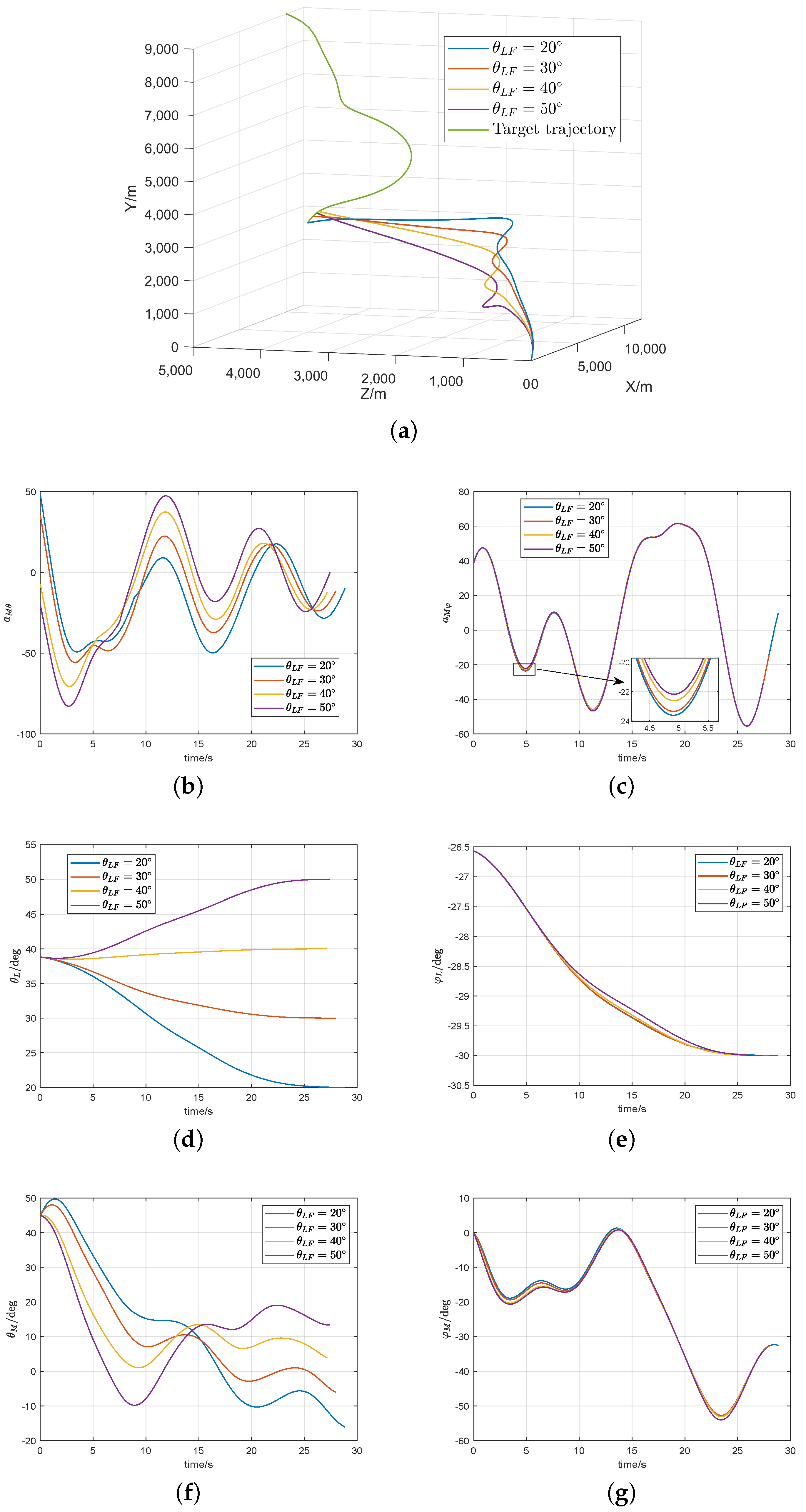
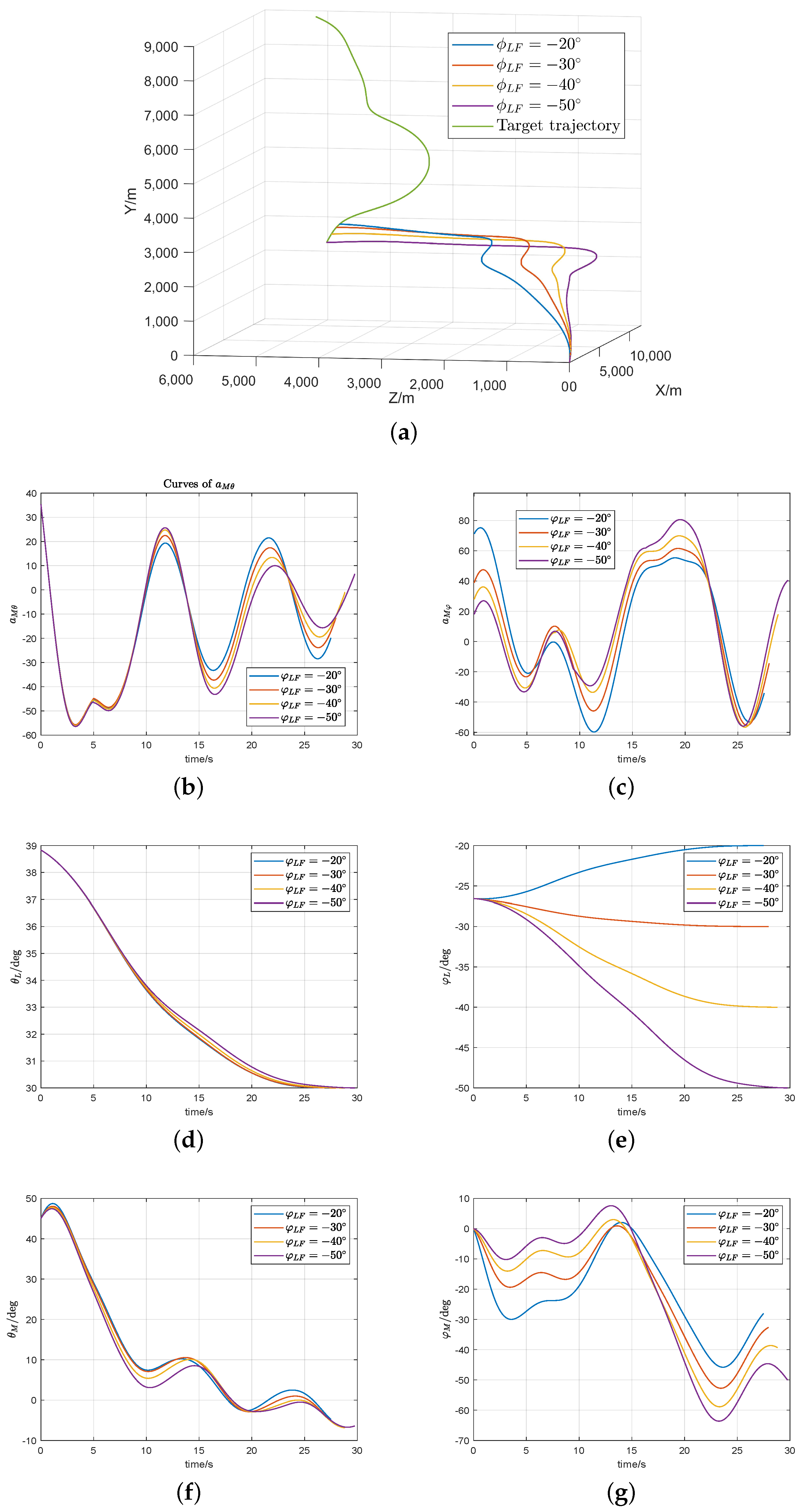
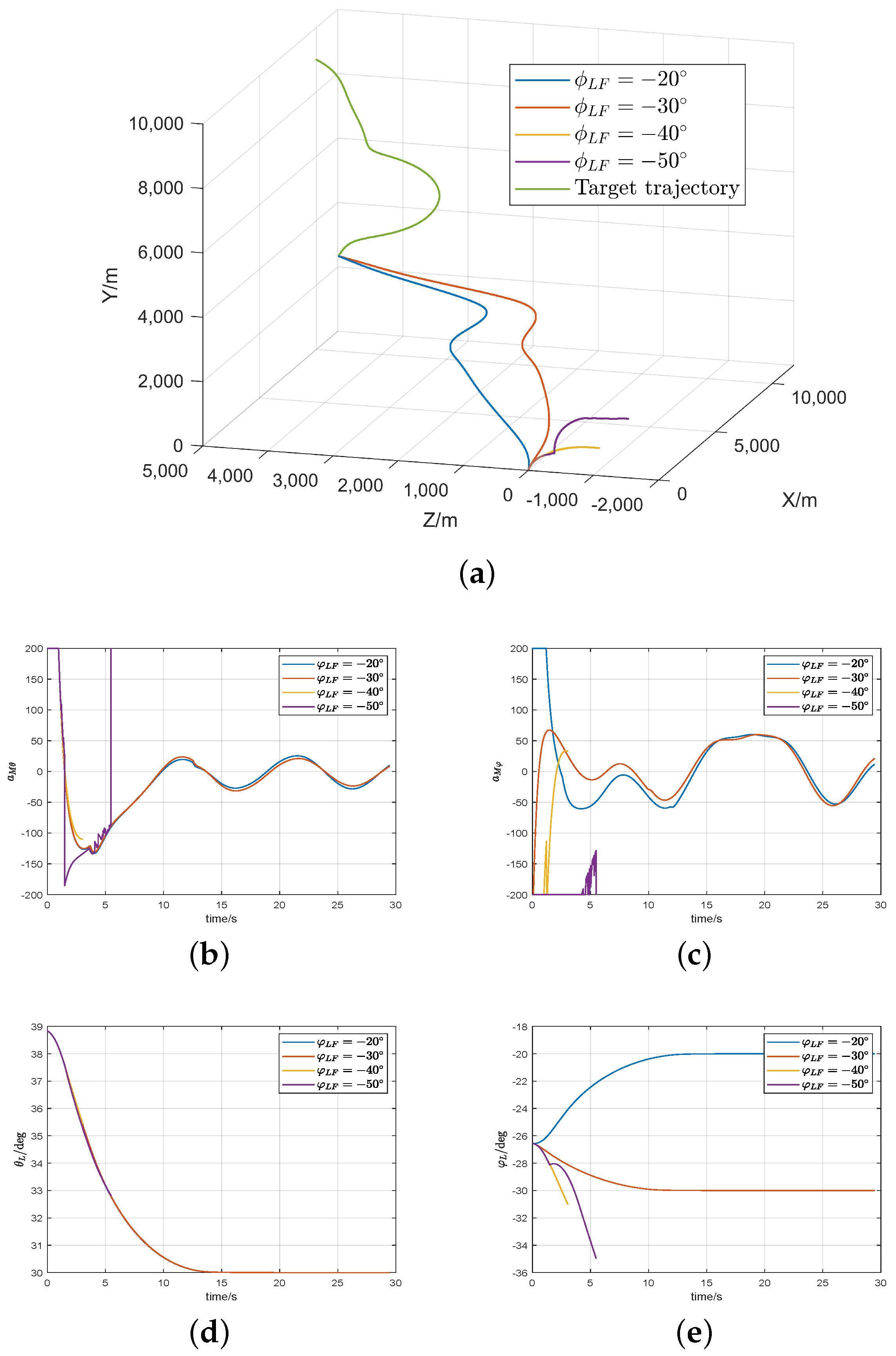
4. Simulation and Analysis

In this section, we conducted various simulations by adjusting the desired LOS angles and altering the target’s maneuvering patterns to different extents, fully verifying the superiority of the proposed guidance law. The initial conditions of the missile and target are shown in

Table 1. Initial simulation conditions.

Parameters	Value
Missile position (m)	(0,0,0)
Target position (m)	(10,000,9000,5000)
Missile speed (m/s)	500
Target speed (m/s)	300
Missile flight path angle (${\theta }_M,{\phi }_M$)	(45,0)
Target flight path angle (${\theta }_M,{\phi }_M$)	(−30,120)

.

The upper bound on the acceleration of the missile is $a_{Mmax}=200\mathrm{m}/{\mathrm{s}}^2$, and the parameters of the designed TBGFTTSM guidance law (40) were set as follows: m = 2, $\kappa$ = 300, c = 15, and $\alpha =0.8$. The parameters of the GSTESO were selected as $\omega =13$.

First, we conducted simulations of our proposed guidance law against a target performing sinusoidal maneuvers, considering different terminal angle constraints. The target acceleration rates were set as $a_{Ty}=60sin\left(0.5t\right)\mathrm{m}/{\mathrm{s}}^2$ and $a_{Tz}=60sin\left(0.5t\right)\mathrm{m}/{\mathrm{s}}^2$. The desired LOS angles are the following conditions:

Case 1: ${\theta }_{Lf}={20}^{\circ },{30}^{\circ },{40}^{\circ },{50}^{\circ }$ when ${\phi }_{Lf}=-{30}^{\circ }$.

Case 2: ${\phi }_{Lf}=-{20}^{\circ },-{30}^{\circ },-{40}^{\circ },-{50}^{\circ }$ when ${\theta }_{Lf}={30}^{\circ }$.

The simulation results are shown in Figure 2 and Figure 3, and the Miss distance and LOS angle errors are shown in

Table 2. Comparative statistics of simulation results for the two guidance laws in Case 1.

	Method	${\mathit{\theta }}_{\mathit{Lf}}={20}^{\circ }$	${\mathit{\theta }}_{\mathit{Lf}}={30}^{\circ }$	${\mathit{\theta }}_{\mathit{Lf}}={40}^{\circ }$	${\mathit{\theta }}_{\mathit{Lf}}={50}^{\circ }$
Miss distance (m)	TBGFTTSM FNTSMGL	0.2779 0.8495	0.2245 0.9794	0.4320 0.8365	0.2066 0.6139
Error of ${\theta }_L$ (°)	TBGFTTSM FNTSMGL	$\mathbf{4.47}\times {\mathbf{10}}^{-\mathbf{8}}$ $2.50\times {10}^{-5}$	$\mathbf{3.17}\times {\mathbf{10}}^{-\mathbf{7}}$ $5.33\times {10}^{-5}$	$\mathbf{1.46}\times {\mathbf{10}}^{-\mathbf{7}}$ $4.22\times {10}^{-5}$	$\mathbf{3.23}\times {\mathbf{10}}^{-\mathbf{7}}$ $5.87\times {10}^{-5}$
Interception time (s)	TBGFTTSM FNTSMGL	28.84 32.69	27.97 29.47	27.42 26.83	27.17 27.66

and

Table 3. Comparative statistics of simulation results for the two guidance laws in Case 2.

	Method	${\mathit{\phi }}_{\mathit{Lf}}=-{20}^{\circ }$	${\mathit{\phi }}_{\mathit{Lf}}=-{30}^{\circ }$	${\mathit{\phi }}_{\mathit{Lf}}=-{40}^{\circ }$	${\mathit{\phi }}_{\mathit{Lf}}=-{50}^{\circ }$
Miss distance (m)	TBGFTTSM FNTSMGL	0.4203 0.9267	0.2245 0.9794	0.1275 13230	0.2876 11707
Error of ${\theta }_L$ (°)	TBGFTTSM FNTSMGL	$-\mathbf{1.06}\times {\mathbf{10}}^{-\mathbf{7}}$ $1.10\times {10}^{-4}$	$-\mathbf{6.13}\times {\mathbf{10}}^{-\mathbf{8}}$ $1.08\times {10}^{-4}$	$-\mathbf{2}.\mathbf{98}\times {\mathbf{10}}^{-\mathbf{7}}$ 8.98	$\mathbf{6}.\mathbf{82}\times {\mathbf{10}}^{-\mathbf{7}}$ 15.05
Interception time (s)	TBGFTTSM FNTSMGL	27.49 29.46	27.97 29.47	28.81 3.05	29.76 5.48

. The proposed guidance law can make the terminal LOS Angle convergence small enough and the normal overload curve smooth without chattering and saturation.

To further compare the performance of the proposed guidance law, we conducted comparisons with the fast nonsingular terminal sliding mode guidance law (FNTSMGL) mentioned in Reference [32]. The expression for this guidance law is defined as follows:

$$\begin{array}{c}{\mathit{s}}_{\mathbf{2}}={\mathit{x}}_{\mathbf{2}}+{\alpha }_1{\mathit{x}}_{\mathbf{1}}+{\alpha }_1{\beta }_1\left({\mathit{x}}_{\mathbf{1}}\right)\hfill \\ {\beta }_1\left({\mathit{x}}_{\mathbf{1}}\right)=\left\{\begin{array}{cc}{\left|{\mathit{x}}_{\mathbf{1}}\right|}^{\gamma }\mathrm{sign}({\mathit{x}}_{\mathbf{1}})& \mathrm{if} \left|{\mathit{x}}_{\mathbf{1}}\right|\ge {\eta }_2\\ b_1{\mathit{x}}_{\mathbf{1}}+b_2{\left|{\mathit{x}}_{\mathbf{1}}\right|}^2\mathrm{sign}(x_1)& \mathrm{if} \left|{\mathit{x}}_{\mathbf{1}}\right|<{\eta }_2\end{array}\right.\hfill \end{array}$$

(51)

where $b_1=(2-\gamma ){\eta }_2^{\gamma -1},b_2=(\gamma -1){\eta }_2^{\gamma -2}$, $\gamma =0.6,{\eta }_2=0.08,{\alpha }_1=0.8$. The FNTSMGL’s expression is

$$\begin{array}{c}\mathit{u}=-{\mathit{B}}^{-1}(\mathit{F}+{\alpha }_1{\mathit{x}}_{\mathbf{2}}+{\alpha }_1{\dot{\beta }}_1\left({\mathit{x}}_{\mathbf{1}}\right)-\overline{\mathit{B}}{\widehat{\mathit{d}}}_{\mathit{T}}-l_1\overline{\mathit{B}}{s}_2-l_2\overline{\mathit{B}}{\left|{\mathit{s}}_{\mathbf{2}}\right|}^{\gamma }\mathrm{sign}\left({\mathit{s}}_{\mathbf{2}}\right))\hfill \\ \overline{\mathit{B}}=\mathit{B}\left[\begin{array}{cc}\mathbf{1}& \mathbf{0}\\ \mathbf{0}& \mathbf{-}\mathbf{1}\end{array}\right]\hfill \end{array}$$

(52)

where $\mathit{B}$ and $\mathit{F}$ are consistent with those in Equation (6).

We selected the same two scenarios to compare with the FNTSMGL.

Figure 4 and Figure 5 and Table 2 and Table 3 illustrate that FNTSMGL is highly susceptible to overload saturation in the initial stage of guidance. Moreover, Figure 4 highlights a significant chattering phenomenon in the guidance commands. And our guidance law’s miss distance is much smaller than the FNTSMGL; even Figure 5 demonstrates a severe miss distance for ${\theta }_{Lf}={30}^{\circ }$ for ${\phi }_{Lf}=-{40}^{\circ }$ and $-{50}^{\circ }$, indicating a substantial deviation from the target.

Figure 6 shows the comparison of the three kinds of observers, in which the Fractional Power Extended State Observer (FPESO) is an observer mentioned in references [32,33,34], and its expression is defined as follows:

$$\begin{array}{c}\left\{\begin{array}{c}\dot{\widehat{\mathit{Z}}}=\mathit{H}-{\lambda }_1\left({\mathit{e}}_{\mathbf{1}}\right)+{\widehat{\mathit{d}}}_T\hfill \\ {\dot{\widehat{\mathit{d}}}}_{\mathit{T}}=-{\lambda }_{2}fal({\mathit{e}}_{\mathbf{1}},{\vartheta }_1,\eta )\hfill \end{array}\right.\hfill \\ fal({\mathit{e}}_{\mathbf{1}},{\vartheta }_1,\eta )=\left\{\begin{array}{cc}{\left|{\mathit{e}}_{\mathbf{1}}\right|}^{{\vartheta }_1}\mathrm{sign}({\mathit{e}}_{\mathbf{1}})& \mathrm{if} \left|{\mathit{e}}_{\mathbf{1}}\right|\ge \eta \\ {\displaystyle \frac{{\mathit{e}}_{\mathbf{1}}}{{\eta }^{1-{\vartheta }_1}}}& \mathrm{otherwise}\end{array}\right.\hfill \end{array}$$

(53)

where ${\lambda }_1=80,{\lambda }_2=800,{\vartheta }_1=0.5,\eta =0.08$.

From Figure 6, it is evident that both the GSTESO and FPESO outperformed the LESO in terms of performance. Particularly noticeable in Figure 6a is that the GSTESO exhibits smaller initial observation errors compared to the FPESO, enabling it to capture the true values more rapidly.

Similarly, we increased the sinusoidal maneuver frequency of the target and introduced two new maneuver types for further testing. Firstly, the frequency was increased fourfold, i.e., $a_{Ty}=60sin\left(2t\right)\mathrm{m}/{\mathrm{s}}^2$ and $a_{Tz}=60sin\left(2t\right)\mathrm{m}/{\mathrm{s}}^2$.

As shown in Figure 7, when the frequency increased, the FPESO failed to accurately estimate the target acceleration. In contrast, our observer continued to perform excellently.

However, in actual guidance processes, the information measured by the seeker may contain noise. Therefore, we incorporated Gaussian noise into the acquisition of the LOS angle rate, with a standard deviation of $\sigma =0.005$ deg/s. The expected LOS angle were set as ${\theta }_{Lf}={30}^{\circ }$ for ${\phi }_{Lf}=-{30}^{\circ }$, and $a_{Ty}=60sin\left(0.5t\right)\mathrm{m}/{\mathrm{s}}^2$, $a_{Tz}=60sin\left(0.5t\right)\mathrm{m}/{\mathrm{s}}^2$.

From Figure 8a,b, we can see that the impact of noise on the GSTESO was slightly less than that on the LESO, but significantly less than on the FPESO. Similarly, for the guidance command, Figure 8c,d illustrate that the GSTESO was smoother than the FPESO and similar to the LESO, without producing excessively large guidance commands at the interception moment like the other two, and it did not produce excessively large guidance commands at the interception moment like the others did. Therefore, Figure 8 indicates that the GSTESO benefits from better measure noise tolerance.

Finally, we introduced a constant maneuvering method for comparison in the simulation for Case 3: $a_{Ty}=40\mathrm{m}/{\mathrm{s}}^2$, and $a_{Tz}=40\mathrm{m}/{\mathrm{s}}^2$.

From Figure 9b,c, it is evident that when faced with simple constant maneuvers, the FNTSMGL still reached overload saturation in the initial phase, whereas our guidance law remained smooth. Figure 9f,g show that the GSTESO could still quickly approach the true values, which is a satisfactory performance.

5. Conclusions

For targets with unknown acceleration, this paper designed a three-dimensional terminal sliding mode guidance law with terminal angle constraints, ensuring finite-time convergence. This sliding mode function is built upon the TBG function, ensuring that the sliding mode system converges to zero at the interception time. Compared to conventional terminal sliding mode guidance laws, the proposed guidance law mitigates initial-phase overload saturation and chattering phenomena in the sliding mode system, resulting in smoother overload commands and enhanced robustness in the control system. In addition, we introduce a novel observer, GSTESO, which possesses stronger robustness and superior estimation capabilities for unknown disturbances compared to the traditional LESO. The finite-time convergence of the closed-loop guidance system has been proven using the Lyapunov stability theory. Comparative simulations with FNTSM guidance laws LESO, and FPESO confirm the aforementioned advantages of our proposed guidance law. In the future, we will conduct research on integrated guidance design and potentially incorporate artificial intelligence techniques such as reinforcement learning, similar to what has been done in references [41,42,43].

References

1. Han, T.; Hu, Q.; Shin, H.-S.; Tsourdos, A.; Xin, M. Sensor-based robust incremental three-dimensional guidance law with terminal angle constraint. J. Guid. Control Dyn. 2021, 44, 2016–2030. [Google Scholar] [CrossRef]
2. Li, K.B.; Su, W.S.; Chen, L. Performance analysis of realistic true proportional navigation against maneuvering targets using Lyapunov-like approach. Aerosp. Sci. Technol. 2017, 69, 333–341. [Google Scholar] [CrossRef]
3. Zhang, W.; Fu, S.; Li, W.; Xia, Q. An impact angle constraint integral sliding mode guidance law for maneuvering targets interception. J. Syst. Eng. Electron. 2020, 31, 168–184. [Google Scholar] [CrossRef]
4. Shima, T.; Golan, O.M. Head pursuit guidance. J. Guid. Control Dyn. 2007, 30, 437–1444. [Google Scholar] [CrossRef]
5. Wei, J.H.; Sun, Y.L.; Zhang, J. Integral sliding mode variable structure guidance law with landing angle constrain of the guided projectile. J. Ordnance Equip. Eng. 2019, 40, 103–105. (In Chinese) [Google Scholar]
6. Zhou, H.; Wang, X.; Bai, B.; Cui, N. Reentry guidance with constrained impact for hypersonic weapon by novel particle swarm optimization. Aerosp. Sci. Technol. 2018, 78, 205–213. [Google Scholar] [CrossRef]
7. Zhang, Y.A.; Ma, G.X.; Wu, H.L. A biased proportional navigation guidance law with large impact angle constraint and the time-to-go estimation. Proc. Inst. Mech. Eng. Part G J. Aerosp. Eng. 2014, 228, 1725–1734. [Google Scholar] [CrossRef]
8. Ma, S.; Wang, X.; Wang, Z.; Yang, J. BPNG law with arbitrary initial lead angle and terminal impact angle constraint and time-to-go estimation. Acta Armamentarii 2019, 40, 68. [Google Scholar]
9. Behnamgol, V.; Vali, A.R.; Mohammadi, A. A new adaptive finite time nonlinear guidance law to intercept maneuvering targets. Aerosp. Sci. Technol. 2017, 68, 416–421. [Google Scholar] [CrossRef]
10. Taub, I.; Shima, T. Intercept angle missile guidance under time varying acceleration bounds. J. Guid. Control Dyn. 2013, 36, 686–699. [Google Scholar] [CrossRef]
11. Li, H.; She, H. Trajectory shaping guidance law based on ideal line-of-sight. Acta Armamentarii 2014, 35, 1200. [Google Scholar]
12. Zhao, J.; Zhou, J. Strictly convergent nonsingular terminal sliding mode guidance law with impact angle constraints. Optik 2016, 127, 10971–10980. [Google Scholar] [CrossRef]
13. Yu, J.; Xu, Q.; Zhi, Y. A TSM control scheme of integrated guidance autopilot design for UAV. In Proceedings of the 3rd IEEE International Conference on Computer Research and Development, Shanghai, China, 11–13 March 2011; Volume 4, pp. 431–435. [Google Scholar]
14. Zhang, Y.; Sun, M.; Chen, Z. Finite-time convergent guidance law with impact angle constraint based on sliding-mode control. Nonlinear Dyn. 2012, 70, 619–625. [Google Scholar] [CrossRef]
15. Kumar, S.R.; Rao, S.; Ghose, D. Nonsingular terminal sliding mode guidance with impact angle constraints. J. Guid. Control Dyn. 2014, 37, 1114–1130. [Google Scholar] [CrossRef]
16. Feng, Y.; Bao, S.; Yu, X. Design method of non-singular terminal sliding mode control systems. Control Decis. 2002, 17, 194–198. (In Chinese) [Google Scholar]
17. Xiong, S.; Wang, W.; Liu, X.; Wang, S.; Chen, Z. Guidance law against maneuvering targets with intercept angle constraint. ISA Trans. 2014, 53, 1332–1342. [Google Scholar] [CrossRef]
18. Zhang, X.; Liu, M.; Li, Y. Nonsingular terminal sliding-mode-based guidance law design with impact angle constraints. Iran. J. Sci. Technol. Trans. Electr. Eng. 2019, 43, 47–54. [Google Scholar] [CrossRef]
19. Kumar, S.R.; Rao, S.; Ghose, D. Sliding-mode guidance and control for all-aspect interceptors with terminal angle constraints. J. Guid. Control Dyn. 2012, 35, 1230–1246. [Google Scholar] [CrossRef]
20. Song, J.; Song, S.; Zhou, H. Adaptive nonsingular fast terminal sliding mode guidance law with impact angle constraints. Int. J. Control Autom. Syst. 2016, 14, 99–114. [Google Scholar] [CrossRef]
21. Yujie, S.I.; Shenmin, S. Three-dimensional adaptive finite-time guidance law for intercepting maneuvering targets. Chin. J. Aeronaut. 2017, 30, 1985–2003. [Google Scholar]
22. Song, Q.Z.; Meng, X.Y. Design and simulation of guidance law with angular constraint based on non-singular terminal sliding mode. Phys. Procedia 2012, 25, 1197–1204. [Google Scholar]
23. He, S.M.; Lin, D.F. Adaptive nonsingular sliding mode based guidance law with terminal angular constraint. Int. J. Aeronaut. Space Sci. 2014, 15, 146–152. [Google Scholar] [CrossRef]
24. Xiong, S.F.; Wang, W.H.; Song, S.Y. Extended state observer based impact angleconstrained guidance law for maneuvering target interception. Proc. Inst. Mech. Eng. Part G J. Aerosp. Eng. 2015, 229, 2589–2607. [Google Scholar] [CrossRef]
25. Ning, B.; Han, Q.-L.; Zuo, Z. Practical fixed-time consensus for integrator-type multi-agent systems: A time base generator approach. Automatica 2019, 105, 406–414. [Google Scholar] [CrossRef]
26. Becerra, H.M.; Vazquez, C.R.; Arechavaleta, G.; Delfin, J. Predefined-time convergence control for high-order integrator systems using time base generators. IEEE Trans. Control Syst. Technol. 2018, 26, 1866–1873. [Google Scholar] [CrossRef]
27. Ning, B.; Han, Q.-L.; Zuo, Z. Bipartite consensus tracking for second-order multiagent systems: A time-varying function-based preset-time approach. IEEE Trans. Autom. Control 2020, 66, 2739–2745. [Google Scholar] [CrossRef]
28. Parra-Vega, V. Second order sliding mode control for robot arms with time base generators for finite-time tracking. Dyn. Control 2001, 11, 175–186. [Google Scholar] [CrossRef]
29. Zhao, Y.; Sheng, Y.; Liu, X. Impact angle constrained guidance for all-aspect interception with function-based finite-time sliding mode control. Nonlinear Dyn. 2016, 85, 1791–1804. [Google Scholar] [CrossRef]
30. Ji, H.; Liu, X.; Song, Z.; Zhao, Y. Time-varying sliding mode guidance scheme for maneuvering target interception with impact angle constraint. J. Frankl. Inst. 2018, 355, 9192–9208. [Google Scholar] [CrossRef]
31. Bai, Y.; Zhang, G.; Wang, Q.; Ding, D.; Li, B.; Wang, G.; Xu, D. High-gain nonlinear active disturbance rejection control strategy for traction permanent magnet motor drives. IEEE Trans. Power Electron. 2022, 37, 13135–13146. [Google Scholar] [CrossRef]
32. Wang, X.; Lu, H.; Huang, X.; Zuo, Z. Three-dimensional terminal angle constraint finite-time dual-layer guidance law with autopilot dynamics. Aerosp. Sci. Technol. 2021, 116, 106818. [Google Scholar] [CrossRef]
33. Zhao, Z.L.; Guo, B.Z. A nonlinear extended state observer based on fractional power functions. Automatica 2017, 81, 286–296. [Google Scholar] [CrossRef]
34. Zhao, Z.L.; Guo, B.Z. A novel extended state observer for output tracking of MIMO systems with mismatched uncertainty. IEEE Trans. Autom. Control 2017, 63, 211–218. [Google Scholar] [CrossRef]
35. Sheikhbahaei, R.; Khankalantary, S. Three-dimensional continuous-time integrated guidance and control design using model predictive control. Proc. Inst. Mech. Eng. Part G J. Aerosp. Eng. 2023, 237, 503–515. [Google Scholar] [CrossRef]
36. Zhao, L.; Gu, S.; Zhang, J.; Li, S. Finite-time trajectory tracking control for rodless pneumatic cylinder systems with disturbances. IEEE Trans. Ind. Electron. 2021, 69, 4137–4147. [Google Scholar] [CrossRef]
37. Lin, D.; Ji, Y.; Wang, W.; Wang, Y.; Wang, H.; Zhang, F. Three-dimensional impact angle-constrained adaptive guidance law considering autopilot lag and input saturation. Int. J. Robust Nonlinear Control 2020, 30, 3653–3671. [Google Scholar] [CrossRef]
38. Han, L.; Mao, J.; Cao, P.; Gan, Y.; Li, S. Toward sensorless interaction force estimation for industrial robots using high-order finite-time observers. IEEE Trans. Ind. Electron. 2021, 69, 7275–7284. [Google Scholar] [CrossRef]
39. Johnson, C.R. Hadamard products of matrices. Linear Multilinear Algebra 1974, 1, 295–307. [Google Scholar] [CrossRef]
40. Liu, S.; Leiva, V.; Zhuang, D.; Ma, T.; Figueroa-Zúñiga, J.I. Matrix differential calculus with applications in the multivariate linear model and its diagnostics. J. Multivar. Anal. 2022, 188, 104849. [Google Scholar] [CrossRef]
41. Chen, W.; Hu, Y.; Gao, C.; An, R. Trajectory tracking guidance of interceptor via prescribed performance integral sliding mode with neural network disturbance observer. Def. Technol. 2024, 32, 412–429. [Google Scholar] [CrossRef]
42. Qiu, X.; Lai, P.; Gao, C.; Jing, W. Recorded recurrent deep reinforcement learning guidance laws for intercepting endoatmospheric maneuvering missiles. Def. Technol. 2024, 31, 457–470. [Google Scholar] [CrossRef]
43. Hu, Z.; Xiao, L.; Guan, J.; Yi, W.; Yin, H. Intercept Guidance of Maneuvering Targets with Deep Reinforcement Learning. Int. J. Aerosp. Eng. 2023, 2023, 7924190. [Google Scholar] [CrossRef]
Figure 1. Relative motion model ( a M is perpendicular to V; a T is perpendicular to V T ).
Aerospace 12 00252 g001
Figure 2. Simulation results for Case 1: (a) trajectories of missile and target; (b,c) missile acceleration commands; (d,e) LOS angle; (f,g) trajectory deviation angle.
Aerospace 12 00252 g002
Figure 3. Simulation results for Case 2: (a) trajectories of missile and target; (b,c) missile acceleration commands; (d,e) LOS angle; (f,g) trajectory deviation angle.
Aerospace 12 00252 g003
Figure 4. Simulation results for FNTSMGL in Case 1: (a) trajectories of missile and target; (b,c) missile acceleration commands; (d,e) LOS angle.
Aerospace 12 00252 g004
Figure 5. Simulation results for FNTSMGL in Case 2: (a) trajectories of missile and target; (b,c) missile acceleration commands; (d,e) LOS angle.
Aerospace 12 00252 g005
Figure 6. Simulation results for three observers: (a) observed value and a M θ ; (b) observed value and a M φ .
Aerospace 12 00252 g006
Figure 7. Simulation results for three observers about a T y = 60 sin ( 2 t ) m / s 2 and a T z = 60 sin ( 2 t ) m / s 2 : (a) observed value and a M θ ; (b) observed value and a M φ .
Aerospace 12 00252 g007
Figure 8. Simulation results for three observers with noise: (a) observed value about θ L ; (b) observed value about φ L ; (c,d) a M under two observer-based guidance laws with noise.
Aerospace 12 00252 g008
Figure 9. Simulation results for FNTSMGL in Case 3: (a) trajectories of missile and target; (b,c) missile acceleration commands; (d,e) LOS angle; (f,g) response of GSTESO.
Aerospace 12 00252 g009aAerospace 12 00252 g009b