Experimental Evaluation of Multi- and Single-Drone Systems with 1D LiDAR Sensors for Stockpile Volume Estimation

Abstract

This study examines the application of low-cost 1D LiDAR sensors in drone-based stockpile volume estimation, with a focus on indoor environments. Three approaches were experimentally investigated: (i) a multi-drone system equipped with static, downward-facing 1D LiDAR sensors combined with an adaptive formation control algorithm; (ii) a single drone with a static, downward-facing 1D LiDAR following a zigzag trajectory; and (iii) a single drone with an actuated 1D LiDAR in an oscillatory fashion to enhance scanning coverage while following a shorter trajectory. The adaptive formation control algorithm, newly developed in this study, synchronises the drones’ waypoint arrivals and facilitates smooth transitions between dynamic formation shapes. Real-world experiments conducted in a motion-tracking indoor facility confirmed the effectiveness of all three approaches in accurately completing scanning tasks, as per intended waypoints allocation. A trapezoidal prism stockpile was scanned, and the volume estimation accuracy of each approach was compared. The multi-drone system achieved an average volumetric error of 1.3%, similar to the single drone with a static sensor, but with less than half the flight time. Meanwhile, the actuated LiDAR system required shorter paths but experienced a higher volumetric error of 4.4%, primarily due to surface reconstruction outliers and common LiDAR bias when scanning at non-vertical angles.

1. Introduction

In recent years, the landscape of geospatial analysis and environmental management has witnessed a transformative shift, driven by the rapid advancements in autonomous unmanned aerial vehicles (UAVs), commonly known as drones. These flying platforms not only allow novel aerospace endeavours [1,2,3,4,5,6,7,8,9], but also have entered various sectors including agriculture [10], forestry [11], and waste management [12], offering innovative solutions to longstanding challenges. Notably, drones have emerged as an effective means of stockpile volume estimation [13,14,15,16,17], a critical activity in industries such as mining [18,19], construction [20,21], and agriculture [10].

The domain of stockpile volume estimation has typically relied on established traditional methods like Terrestrial Laser Scanning (TLS) and Global Navigation Satellite Systems (GNSSs), as industry standards. In fact, TLS has become a prime choice in industry due to its straightforward operation and the sub-centimetre accuracy it can achieve. However, it is often viewed as an expensive approach, especially when surveying large and complex surfaces. This is because it necessitates frequent repositioning of the sensors to minimise occlusion thereby ensuring sufficient data collection, a process that potentially poses personnel risks in hard-to-reach or dangerous environments. On the other hand, GNSS surveying involves the collection of singular points around and over the area of interest, and the accuracy of the modelled surfaces is typically enhanced as more points are collected. However, it requires surveyors to navigate and climb stockpiles to position the GNSS receiver(s) over the measurement points, a procedure that is dependent on the suitability of the inspection environment. Despite the costs associated with both methods that make them less ideal for frequent surveys or smaller operations, they have retained their position as industry standards. For more details on these methods, the reader is referred to the review work [13].

Recognising the previous challenges of danger and cost, there has been a significant shift towards integrating UAV technology into stockpile volume estimation tasks. This approach builds on the potential advantages that UAVs can offer including efficiency, safety, and accuracy. In fact, over the past decade, drone photogrammetry has asserted itself as a reliable and efficient method for stockpile volume estimation in outdoor environments. This technique has been validated through numerous studies, showcasing acceptable accuracy and offering significant improvements over traditional methods [14,22,23,24,25]. Notably, most studies have reported volumetric errors in the range of $\approx 0–3\%$ when compared to results from TLS, GNSS, or actual known volumes [13]. However, the drone solution does not come without its challenges: the accuracy of volume estimation using drone photogrammetry can be significantly influenced by various factors, including the quality of captured images [26], the grid size utilised in 3D surface generation [27], ground control point (GCP) placement, and the flight altitude of the drone [28].

Despite the significant progress in stockpile volume estimation within outdoor/open environments, the domain of indoor stockpile volume estimation remains relatively underexplored whilst presenting several unique challenges. In particular, current methods often struggle in confined spaces, where issues such as poor visibility, dust, and uneven terrain increase the complexity of the stockpile inspection and volume estimation process. In these circumstances, Light Detection and Ranging (LiDAR) technology emerges as a better choice over image-based methods. In fact, LiDAR sensors (which employ a laser to measure distances and create detailed 3D models) have found applications across diverse fields including agriculture [29] and mining [30], and recent studies have started to apply them for the stockpile volume estimation application, exploring various platforms ranging from aerial [31] to rail-mounted [32] systems. In fact, LiDAR emerges as a better choice over image-based methods, particularly in dusty and dark environments where visibility issues can severely impact the effectiveness of photogrammetric methods [33], as is often the case in indoor environments.

In this study, we demonstrate indoor stockpile scanning with 1D LiDAR sensors while using a new adaptable multi-drone formation control to achieve the desired formation. This multi-drone approach merges the efficiencies of using individual drones into a cohesive, collaborative unit, optimising the coverage of the designated area while ensuring cost-effectiveness, fault tolerance, and reliability. Moreover, implementing a multi-agent drone system allows for the deployment of micro drones, which can inspect areas with minimal environmental impact due to their smaller size. This feature is particularly advantageous if a drone is lost or collides with an object, as the smaller batteries reduce the risk of significant damage or explosions. Here, we consider and experimentally assess previously proposed approaches, including indoor stockpile scanning with a single drone equipped with an actuated 1D LiDAR [34], a concept that has so far only been validated through computer simulations, as well as the typical approach of utilising a single drone with a vertical 1D LiDAR navigating a zigzag path pattern [17]. We show that by using 1D LiDAR scanners, we can achieve acceptable accuracy while maintaining low cost and weight.

The current study presents the first experimental assessment of the different possible 1D LiDAR drone-based approaches to the application at hand and hence offers the scientific community as well as practitioners valuable insights. Scientifically, this work develops a novel adaptive multi-drone formation control and path planning algorithm suitable for micro drones, offers an informative comparative analysis based on experimental assessment for the different drone-based scanning approaches under similar conditions, and investigates the accuracy of the estimated volume from each method. For practitioners, this paper experimentally demonstrates the implementation of newly developed scanning techniques for indoor stockpile volume estimation, evaluates and compares the different low-cost LiDAR-based approaches, and provides detailed methodologies and results that practitioners can implement and adapt to their own operations. To put more focus on the novel aspects of the current work, this study represents the first experimental evaluation of various drone-based scanning methods in a controlled environment, enhancing the reliability of comparisons. This research uniquely investigates small and multi-drone approaches for stockpile volume estimation. Unlike previous studies that focus on outdoor settings using heavier and costlier 2D and 3D LiDAR systems [31,35,36], this work showcases how lightweight 1D LiDAR sensors can achieve acceptable coverage whilst retaining cost-effectiveness. In fact, the methods demonstrated in this research effectively compete with the traditional, more expensive systems, marking a useful contribution to the field. Moreover, while a single drone equipped with a gimballed or 3D LiDAR might provide a robust solution, such systems are often heavy and require larger drones, which pose safety concerns in indoor environments. As highlighted earlier, micro drones typically cannot carry such payloads or sustain long-duration missions due to battery limitations. By leveraging a multi-drone system with lightweight 1D LiDAR sensors, our approach ensures complete coverage of large indoor environments while maintaining cost-effectiveness and safety. In addition to providing redundancy and operational flexibility, this method minimizes the risks associated with larger, more complex systems, making it a practical and scalable solution for indoor stockpile volume estimation.

While safety concerns regarding drones in industrial indoor environments are valid, their benefits in confined space inspections and stockpile measurements are significant. A drone named Elios 3 [37], for example, has been successfully deployed in hazardous settings like cement plants, improving safety, efficiency, and accuracy where manual methods are impractical. Modern drones also incorporate safety features like protective cages, aligning with our approach. Just as drone-based outdoor mapping evolved into an industry standard, indoor applications are following a similar trend. While commercial solutions exist, they remain costly, and our research seeks to explore a more affordable alternative, making drone-based indoor stockpile measurement a practical and necessary innovation rather than a passing trend.

The subsequent sections of this paper are structured as follows: Section 2 presents the 1D LiDAR drone-based approaches considered for indoor stockpile volume estimation missions, particularly emphasising the multi-drone solution, including formation control and path planning. This is followed by Section 3, which demonstrates the experimental work involved, detailing the setup, the point cloud generation process, the single-point LiDAR scanner, the reference stockpile configuration, and the data collection methodology. In Section 4, we detail the study’s findings, including the analysis of the performance of the proposed approaches. Finally, Section 5, summarises the conclusions and future work recommended from our investigation.

2. 1D LiDAR Drone-Borne Approaches for Stockpile Volume Estimation

2.1. Overview

Building upon insights gathered from our previous studies [17,34,38], we recognise that a solo or a multi-drone system equipped with a single 1D LiDAR sensor can, with the aid of an external localisation system, achieve an acceptable level of accuracy in volume estimation that is comparable to estimates obtained from the more sophisticated and more expensive 2D/3D LiDAR sensors. Leveraging the lightweight characteristics of 1D LiDAR sensors, they can be integrated into micro drones, hence not only enabling better feasibility but also significantly enhancing safety within geometrically constrained indoor environments as opposed to deploying larger drones. That said, it should be noted that the use of micro drones also brings across the challenge of restricted battery capacity for comprehensive coverage.

The approaches examined in this study vary based on different factors. The first factor considered in this study is the number of platforms, i.e., compare the performance indexes when multi-drone and single-drone approaches are employed. The second factor is the trajectory shape and how it affects the coverage performance while ensuring the best comparable setting for each approach. The third factor is the type of 1D LiDAR used, specifically whether the 1D LiDAR is static and facing downward toward the ground or actuated/oscillating, and how this affects the accuracy of the reconstructed stockpile. The following sub-sections will introduce the employment of multi-drone agents with static 1D LiDAR, discuss scanning using a single drone equipped with an actuated 1D LiDAR, and highlight the use of a single drone with a static 1D LiDAR.

2.2. Multi-Drone Agents with Static 1D LiDAR Sensors

In the first approach considered here, we propose a dynamic formation control algorithm characterised by robustness in formation shapes and waypoints tracking. The core idea of this developed algorithm is to synchronise the arrival time of the multiple drones at their corresponding locations, ensuring a coordinated and simultaneous arrival. The algorithm starts with computing the path length for each drone from its current position to its next desired position at the next waypoint and identifies the longest path length. This evaluation of the longest path length, together with the knowledge of the maximum velocity permitted, enables an estimation of travel duration that would be used to synchronise the speed of all drones to ensure they simultaneously reach the desired formation shape at the next waypoint. In other words, the drone with the longest distance to its next desired position will move at maximum speed, while the one with the shortest distance will move at minimum speed, and both would have the same travel duration.

The target position for each drone is determined by combining the desired waypoint with the desired formation shape at that waypoint. In the initial phase of the dynamic formation control algorithm, the task is to determine the target positions ${\mathit{P}}^{\mathrm{target}}\in {\mathbb{R}}^{\mathbb{3}}$ (where ${\mathbb{R}}^3$ represents three-dimensional space) for each drone $i$ at every waypoint ${\mathit{W}}_k\in {\mathbb{R}}^{\mathbb{3}}$ using the desired formation shape ${\mathit{H}}_k\in {\mathbb{R}}^{\mathbb{3}}$. As such, mathematically, the target position for each drone $i$ can be represented as:

$${\mathit{P}}_i^{\mathrm{target}}={\mathit{H}}_{k,i}+{\mathit{W}}_k,$$

(1)

where ${\mathit{H}}_{k,i}$ is the $i^{th}$ drone position in the formation topology associated with the waypoint ${\mathit{W}}_k$. The formation topologies are characterised by a set of relative values to the first drone with $i=1$. Then, the Euclidean distance or path length $d$ between the initial position ${\mathit{P}}^{\mathrm{initial}}$ and the target position ${\mathit{P}}^{\mathrm{target}}$ for each drone $i$ in a multi-dimensional space is calculated as:

$$d_i={‖{\mathit{P}}_i^{\mathrm{target}}-{\mathit{P}}_i^{\mathrm{initial}}‖}_2,$$

(2)

where $‖ .‖$ is the 2-norm or Euclidean norm, and ${\mathit{P}}_i^{\mathrm{target}}$ and ${\mathit{P}}_i^{\mathrm{i}\mathrm{n}\mathrm{i}\mathrm{t}\mathrm{i}\mathrm{a}\mathrm{l}}$ represent the target and initial positions of the $i$^th drone, respectively. The maximum path length, $d_{\max }\in \mathbb{R}$, which we use to harmonise the speed of all drones, is then determined as:

$$d_{\max }=\max (d_1,{ d}_2, \cdots ,{ d}_m),$$

(3)

where $m$ is the number of drones within the swarm. The travel duration, $T$, required for all drones to reach their next target position while forming the desired shape is then given by:

$$T={\displaystyle \frac{d_{\max }}{v_{\max }}} ,$$

(4)

where $v_{\max }$ is the maximum desired velocity, set by the user. Subsequently, the position of each drone ${\mathit{P}}_i$ at any given time $t$ during the transition can be modelled as:

$${\mathit{P}}_i\left(t\right)={\mathit{P}}_i^{\mathrm{initial}}+\left({\displaystyle \frac{t}{T}}\right)·\left({\mathit{P}}_i^{\mathrm{target}}-{\mathit{P}}_i^{\mathrm{initial}}\right) .$$

(5)

Next, we present a numerical demonstration to illustrate the efficiency and robustness of the developed dynamic/adaptive formation control algorithm. In this demonstration, we consider a scenario involving three drones (hence, $m=3$) navigating through three waypoints defined in the 3D coordinate space: ${\mathit{W}}_1=\left\{\mathrm{0,5},0\right\}$, ${\mathit{W}}_2=\left\{5,5,0\right\}$, and ${\mathit{W}}_3=\{5,0,0\}$. Initially, all drones are positioned at the origin. The formation topologies are defined as:

$${\mathit{H}}_{i=1:3}^k=\left[\begin{array}{c}{\mathit{H}}_1^k\\ {\mathit{H}}_2^k\\ {\mathit{H}}_3^k\end{array}\right],$$

(6)

and, for our current numerical example, can be written as:

$${\mathit{H}}_{i=1:3}^{k=1}=\left[\begin{array}{ccc}0& 0& 0\\ 1& -1& 0\\ 2& -2& 0\end{array}\right], {\mathit{H}}_{i=1:3}^{k=2}=\left[\begin{array}{ccc}0& 0& 0\\ -1& -1& 0\\ -2& -2& 0\end{array}\right], {\mathit{H}}_{i=1:3}^{k=3}=\left[\begin{array}{ccc}0& 0& 0\\ -1& 0& 0\\ -2& 0& 0\end{array}\right].$$

(7)

Each row in $\mathit{H}$ presents the 3D relative position of a drone, with the first row describing the reference drone’s position. Moreover, the Z-values are set to zero to facilitate a 2D representation, avoiding potential confusion that might arise from a 3D demonstration. Note that, here, we have set the maximum velocity to $v_{\mathrm{m}\mathrm{a}\mathrm{x}}=0.1$ m/s, with path updates occurring at a frequency of 10 Hz. This maximum velocity was chosen because the tests are typically conducted in a small indoor area using micro drones, and the lower maximum speed hence ensures precise control and manoeuvrability within the confined space, minimising the risk of collisions. Moreover, the path update frequency of 10 Hz was selected based on real-world testing, as it provided stable and reliable data transfer for controlling the drones by sending the desired positions at a rate that ensures smooth movement.

To assess the algorithm’s performance, we introduce a metric, $P_i^{\mathrm{error}}\left(t\right)$, which calculates the difference between the $i^{th}$ drone current and target positions at any time instant $t$. Hence, it is defined as:

$$P_i^{\mathrm{error}}\left(t\right)={‖{\mathit{P}}_i^{\mathrm{target}}-{\mathit{P}}_i\left(t\right)‖}_2.$$

(8)

Furthermore, we define another metric, $F^{\mathrm{error}}\left(t\right)$, to assess the formation shape over time. This metric compares the current inter-drone distances with the distances dictated by the desired formation, where the current distances vector, ${\mathit{F}}^{\mathrm{current}}\left(t\right)\in {\mathbb{R}}^{\mathbb{3}}$, and the target distance vector, ${\mathit{F}}^{\mathrm{target}}\in {\mathbb{R}}^{\mathbb{3}}$, are computed as follows:

$$P_i^{\mathrm{error}}\left(t\right)={‖{\mathit{P}}_i^{\mathrm{target}}-{\mathit{P}}_i\left(t\right)‖}_2,$$

(9)

$${\mathit{F}}^{\mathrm{target}}=\left[{\mathit{H}}_{i=2}^k-{\mathit{H}}_{i=1}^k{,\mathit{H}}_{i=3}^k-{\mathit{H}}_{i=2}^k{,\mathit{H}}_{i=1}^k-{\mathit{H}}_{i=3}^k\right] .$$

(10)

As such, the formation shape error, $F^{\mathrm{error}}\left(t\right)$, is then computed as the mean absolute difference between ${\mathit{F}}^{\mathrm{current}}\left(t\right)$ and ${\mathit{F}}^{\mathrm{target}}$, and is given by:

$$F^{\mathrm{error}}\left(t\right)={\displaystyle \frac{1}{m}}\sum \left|{\mathit{F}}^{\mathrm{current}}\left(t\right)-{\mathit{F}}^{\mathrm{target}}\right|,$$

(11)

where $\left| .\right|$ denotes the absolute value. Finally, to demonstrate that the developed formation algorithm ensures consistency and smooth transitions between different formation shapes, we evaluate the relative distance, $d_i^{\mathrm{relative}}\left(t\right)\in \mathbb{R}$, between each drone’s current position, ${\mathit{P}}_i\left(t\right)$, and the desired position of drone 1 at time $t$ in the planned path by the algorithm, using:

$$d_i^{\mathrm{relative}}\left(t\right)={‖{\mathit{P}}_i\left(t\right)-{\mathit{P}}_1\left(t\right)‖}_2.$$

(12)

The numerical demonstration results are shown in Figure 1. Figure 1a shows the journey of the three drones/agents, initiating from the origin and gradually adopting the target formation shape en route to the first waypoint. Subsequently, they manoeuvre to the next waypoint, seamlessly transitioning into the subsequent formation shape. As such, this figure serves as a visual demonstration of the algorithm’s ability to enable linear transitions between different formation shapes while navigating from one waypoint to another, effectively demonstrating the dynamic formation shape-changing capability of the algorithm. Figure 1b shows the $P^{\mathrm{error}}$ metric for each drone, demonstrating the positional error over time and highlighting the synchronisation in the arrivals at the waypoints. Complementing this, Figure 1c presents the formation error metric $F^{\mathrm{error}}$, showcasing a marked reduction as the drones approach the next waypoints. Finally, Figure 1d illustrates the smooth variation in the $d_i^{\mathrm{relative}}$ metric, confirming the formation consistency and ensuring smooth transitions between different formation shapes.

The demonstration in Figure 1 showcased that the developed algorithm allows for smooth transitions between different formation shapes, minimising the time required for formation adjustments and ensuring a seamless and fluid movement of the swarm. Here, it should be noted that the algorithm proposed in this study is designed to be highly adaptable and independent of specific factors such as the stockpile geometry, workspace conditions, and drone performance. Moreover, the proposed approach extends beyond the current study as the proposed formation control lays the groundwork for possible future enhancements, such as incorporating obstacle avoidance systems that allow one drone to detect and communicate to the entire formation, updating their paths accordingly. Finally, in cases where a drone is lost or fails, the formation control algorithm can adapt the topology in real time, redistributing the remaining drones to ensure continued optimal coverage.

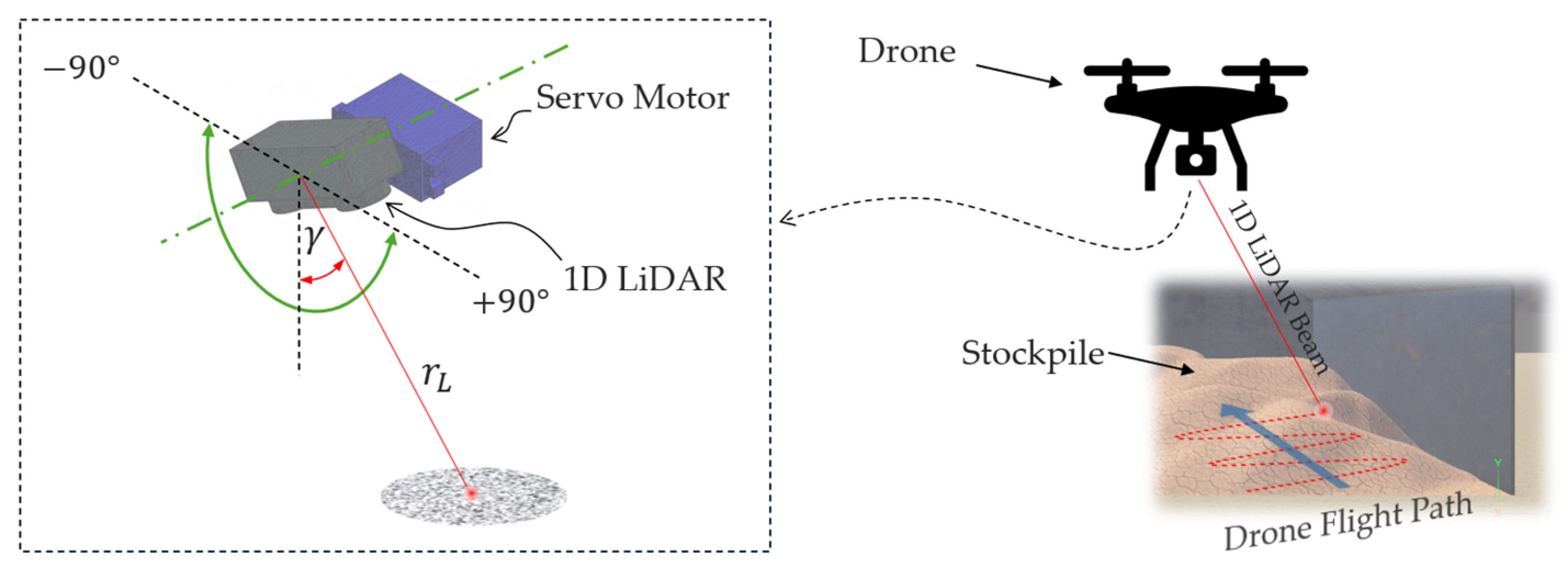
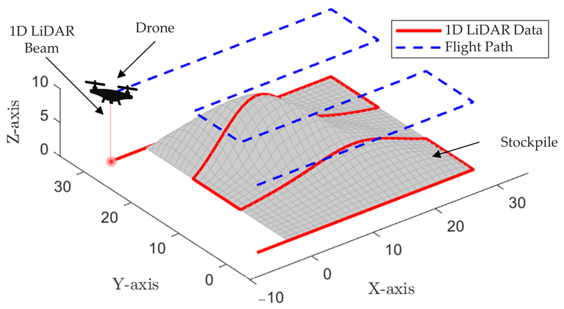
2.3. Single Drone with an Actuated 1D LiDAR Sensor

To compare the new multi-drone approach with previously demonstrated methods, we consider the 1D-actuated LiDAR approach developed by Alsayed and Nabawy [34]. This approach was extensively tested through simulations but had not been experimentally evaluated. As such, in this paper, we will assess and test this method experimentally. In brief, the approach utilises a micro servo motor fitted on a small drone to actuate the 1D LiDAR in an oscillatory fashion about one axis, as illustrated in Figure 2. The servo motor oscillation is within ±90° in a plane perpendicular to the drone’s forward motion. Unlike the multi-drone approach, which requires coverage of many desired points to ensure acceptable stockpile reconstruction quality, this approach benefits from the actuation of the LiDAR to significantly enhance the scanning coverage. Consequently, only four waypoints, located at the corners of the desired area to be scanned, are deemed sufficient for the drone to follow. For a full explanation of the approach, the reader is referred to [34] for details.

2.4. Single Drone with Static 1D LiDAR Sensor

The third approach considered in this paper is the most traditional drone-based approach. It was first developed and presented to address the stockpile volume estimation application in [17]. This approach employs the same scanning method as the multi-agent approach, utilising a single-point static LiDAR facing the ground. However, unlike the multi-drone approach, where multiple drones cover the area of interest within a single round, this approach requires the drone to follow a zigzag pattern path to ensure sufficient coverage of the area to be scanned. This is mainly due to the use of a single drone and the static nature of the LiDAR sensor, which lacks the enhanced scanning coverage provided by the actuated LiDAR. However, on the positive side, this approach offers a low-cost solution for stockpile volume estimation within confined spaces. Figure 3 shows a visual illustration of the approach, depicting a drone with a 1D LiDAR facing the ground to collect data.

2.5. Point Cloud Generation and Registration

Once a surveying mission is finished, to create a representation of the surveyed area, the data harvested through the Time-of-Flight (ToF) sensor (1D LiDAR) is processed via transformation. This stage, known as point cloud registration, involves converting data from the drone’s individual local coordinate frame, $L$, to a single global reference frame, $G$. This mathematical transformation of the point cloud data is given by:

$$\mathit{P}{\mathit{C}}_G=\mathit{R}\times {\mathit{P}}_L+\mathit{T},$$

(13)

where $\mathit{P}{\mathit{C}}_G\in {\mathbb{R}}^{\mathbb{3}\times 1}$ denotes the registered point cloud represented within the ground frame; $\mathit{R}$ $\in {\mathbb{R}}^{\mathbb{3}\times 3}$ is a rotation matrix from the local coordinate frame, $L$, to the global reference frame, $G;\mathit{T}\in {\mathbb{R}}^{\mathbb{3}\times 1}$ is the translation vector that represents the drone/LiDAR position in the global frame; and ${\mathit{P}}_L\in {\mathbb{R}}^{\mathbb{3}\times 1}$ denotes the measured range in the drone/LiDAR 3D coordinate local frame, defined as ${\mathit{P}}_L=\left[0,0,-r_L\right]$ when employing a static 1D LiDAR, and as ${\mathit{P}}_L=[0,{-r}_L \cos (\gamma ), {-r}_L \sin (\gamma \left)\right]$, where $\gamma$ represents the angular displacement measured from the servo motor’s vertical position when considering an actuated 1D LiDAR. Here, $r_L$ is the measurement derived from the onboard rangefinder, indicating the distance beneath the drone, hence the negative sign, which accounts for the downward orientation of the rangefinder.

The rotation matrix $\mathit{R}$ was constructed utilising the drone’s dynamics during navigation (the drone’s roll, pitch, and yaw angles) gathered from the data of the motion tracking system (for a full definition of the rotation matrix, the reader is referred to our previous works [17,34]). Consequently, each point ${\mathit{P}}_L$ is mapped to its corresponding global position using the drone’s global position in the translation vector $\mathit{T}$, which is extracted from the data acquired through the motion tracking system.

To generate a stockpile surface from the point cloud ($\mathit{P}{\mathit{C}}_G$), a MATLAB script was developed. This script creates a mesh grid based on the scanned area $X$ by $Y$, and uses cubic interpolation via the ’griddata’ function to create a surface passing through the point cloud. To determine the volume beneath this 3D surface, the trapezoidal rule was applied. Hence, the volume is calculated using the following formula:

$$V_{\mathrm{s}\mathrm{t}\mathrm{o}\mathrm{c}\mathrm{k}\mathrm{p}\mathrm{i}\mathrm{l}\mathrm{e}}=\sum _{A=1}^{\alpha -1}\sum _{B=1}^{\beta -1}{\displaystyle \frac{1}{4}}\mathsf{\Delta }X\mathsf{\Delta }Y\left(Z_{AB}+Z_{A\left(B+1\right)}+Z_{\left(A+1\right)B}+Z_{\left(A+1\right)\left(B+1\right)}\right),$$

(14)

where $V_{\mathrm{stockpile}}$ represents the total volume and $\Delta X$ and $\Delta Y$ are the grid sizes in the $X$ and $Y$ directions, respectively. The term $Z_{ij}$ represents the height value at the grid cell ($A$, $B$). The double summation is performed over all $A$ and $B$ indices, with $A$ ranging from 1 to $\alpha$ and $B$ ranging from $1$ to $\beta$, where $\alpha$ and $\beta$ are the maximum indices in the $X$ and $Y$ directions, respectively. This covers all grid cells within a defined area. Note that $\Delta X$ and $\Delta Y$ were set to 0.05 m following a sensitivity analysis, which demonstrated that using smaller grid sizes does not affect the accuracy of the obtained results.

It is important to mention that LiDAR data can suffer issues such as noise and bias errors. However, this study only employs 1D LiDAR sensors, which are generally less affected by noise and bias compared to 2D and 3D systems, due to their simpler design [39]. Additionally, LiDAR measurements can be influenced by the material properties of the scanned surfaces—such as reflectivity and texture—which may further affect accuracy. To mitigate these effects, calibration and pretests were performed to eliminate and correct any potential bias arising from material characteristics. Notably, for the case of the actuated 1D LiDAR approach, tests were also conducted with the drone positioned stationery to check the preciseness of the data collection process. During these tests, the servo motor oscillated, demonstrating the generation of a robust dataset with high correlation across the oscillation cycles. Furthermore, to eliminate any potential source for bias, preliminary flights of all drone platforms were performed over a flat surface. These flights enabled the comparison of the LiDAR readings to the motion tracking system altitude readings, hence ensuring the elimination of any potential biases. We did observe some residual noise in the generated point clouds, particularly in the actuated approach when using the servo motor; therefore, we applied MATLAB’s point cloud denoise function (pcdenoise) from the Computer Vision Toolbox in MATLAB R2023b to further enhance the results.

3. Experimental Work

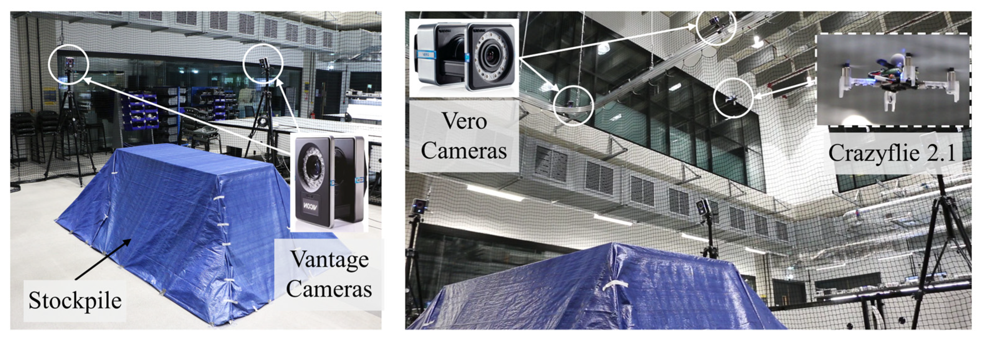
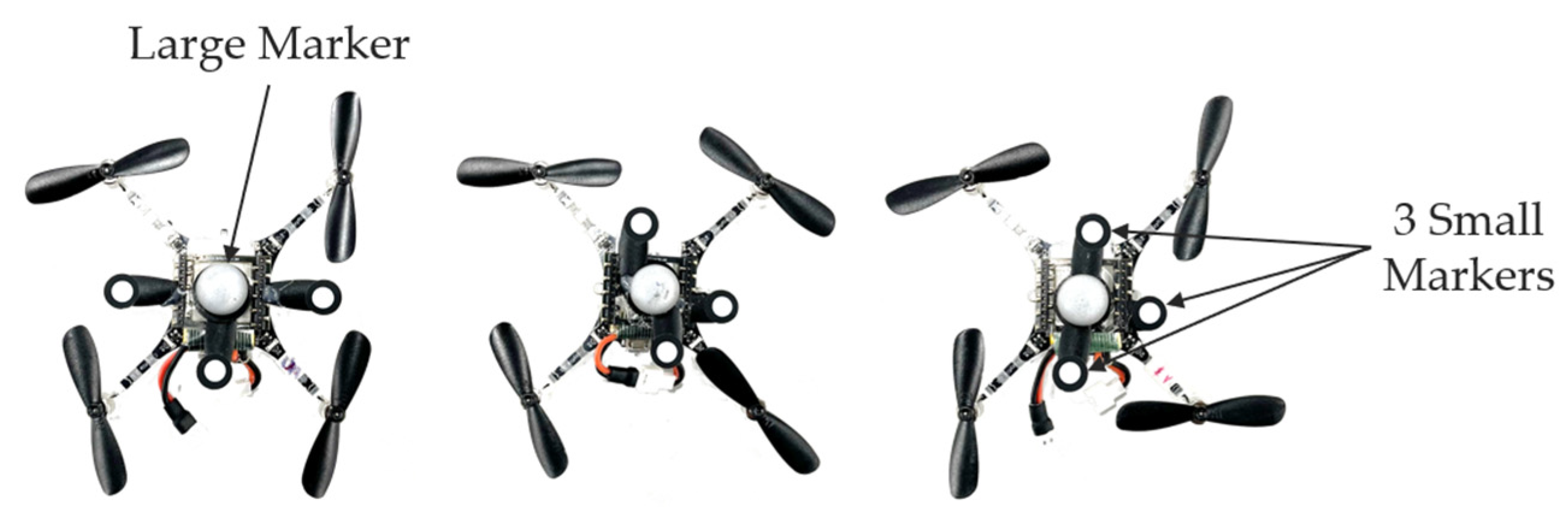
3.1. Setup for Multi-Drone Agents and Single-Drone with Static 1D LiDAR Sensors

To compare the performance of the discussed three approaches in Section 2, we conducted an experimental investigation in a netted drone flight test enclosure at the University of Manchester’s School of Engineering (Figure 4). Within this enclosure, an advanced VICON motion tracking system, known for its precision in 3D tracking (Vicon Motion Systems Ltd, Oxford, UK [40]), was installed. This system utilised 18 cameras positioned at different heights to capture data, and these captured data were processed using a Vicon-supplied PC through its proprietary software, Tracker 3.10.

For the experiments, we employed Crazyflie 2.1 drones (Bitcraze, Malmö, Sweden [41]), known for their lightweight (27 g) and compact, open-source design, Figure 5. These drones can enable a maximum flight duration of approximately 7 min. Hence, at a flight speed of 1 m/s, the drone can cover a distance of over 400 m within this time frame, which is more than sufficient for the experimental tests conducted. However, the drone can easily be replaced with one that has a larger battery capacity if the task requires extended flight time. The drones were equipped with a flow deck for enhanced stability, which also uses an integrated 1D LiDAR sensor to collect surface data beneath the drone [42]. Note that the experimental tests conducted by Kilberg et al. demonstrated that this integrated LiDAR provides highly accurate results, with plots comparing the ground truth to the sensor data [43]. These data, hence, serve as the foundational element in scanning ground structures and stockpiles. Therefore, a 3D surface can be generated, and the volume underneath the surface can be estimated. Operations were directed from a ground station laptop, which communicated with the multiple drones via a radio dongle and accessed real-time drone positioning data through a Robot Operating System (ROS) package, “vicon_bridge [44]”, facilitating the interface with the Vicon system, Figure 6.

For our tests, a custom-developed Python 3.10 code (provided in Supplementary Material) was written utilising the Crazyflie Python library [45] and operated in the following sequence:

• Initialisation of dedicated log files for each drone, cataloguing timestamp, position and orientation (sourced from the VICON system), desired positions, and depth range;
• ROS node activation to launch VICON data reception, which is simultaneously recorded in the log file via a distinct thread;
• Establishing connectivity with drones and updating the drones’ position estimator with their current positions from the VICON system;
• Execution of a closed-loop function, operating at 10 Hz, which constantly feeds the desired trajectory from the formation control to the drone’s desired position function in the Crazyflie Python library. Concurrently, it updates the drone position estimator using the VICON data.

It is important to highlight that initially, the drone’s Z-position (altitude) did not update within the Python code described above due to issues with the Kalman filter. The Kalman filter fuses data from the multiple drone sensors to determine its precise location. However, in this case, the filter gave excessive weight to the depth sensor readings, rather than the VICON data for altitude adjustments. Such weighting led to compromised stability, causing erratic altitude shifts. In many instances, these unpredictable variations resulted in crashes, especially when the drone flew over objects and edges that represent sudden changes in the depth distance beneath it. To mitigate this issue, we modified the firmware of the Crazyflie drone to exclude the rangefinder’s influence on altitude adjustments. This ensured that the rangefinder’s data were not incorporated into the position estimation process within the Kalman filter.

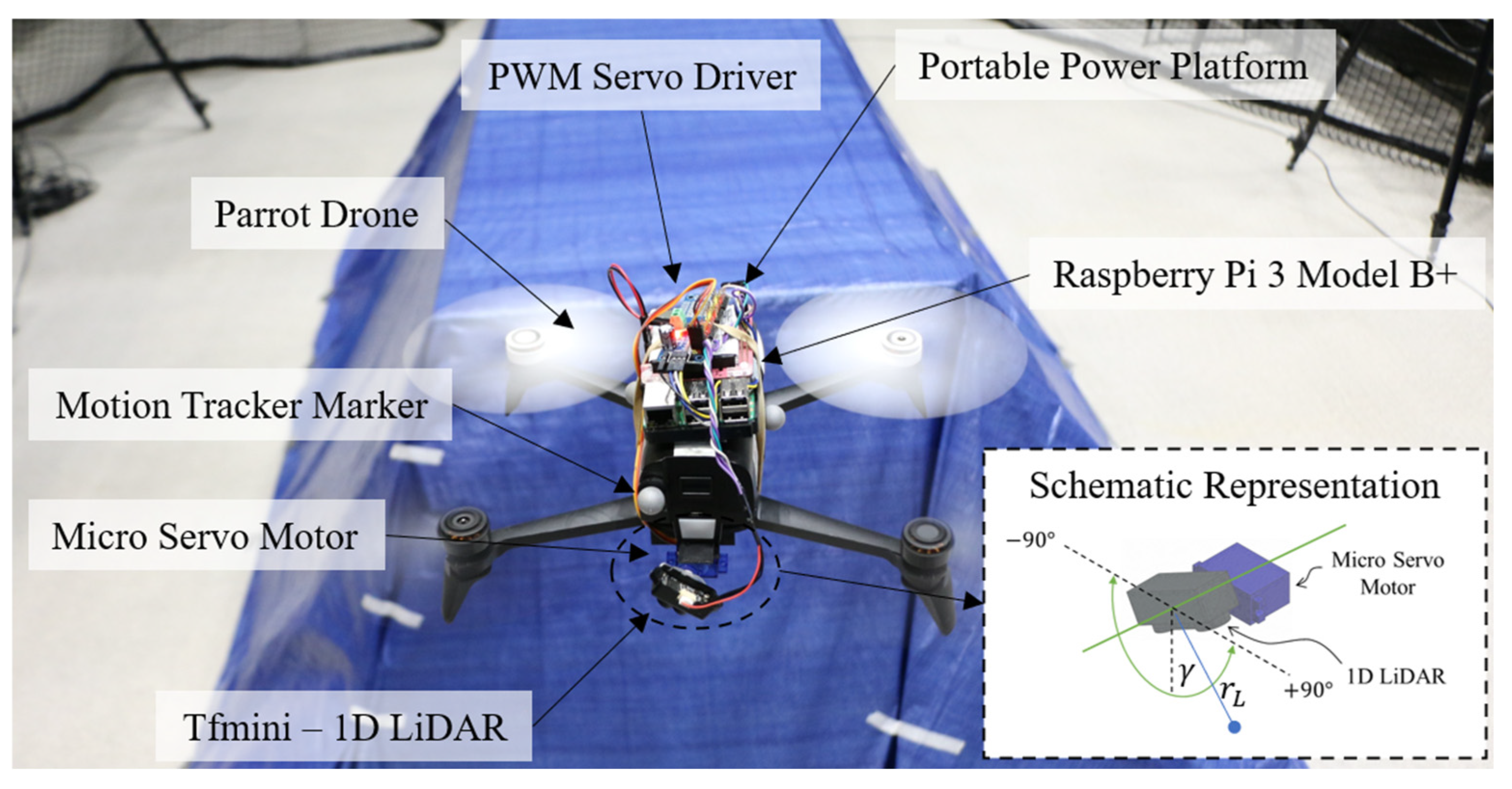
3.2. Setup for the Single Drone with the Actuated 1D LiDAR Sensor

In this section, we explain the setup developed to realise the approach employing a single drone with an actuated 1D LiDAR sensor (Figure 7). Note that given the small size and limited payload capacity of the Crazyflie micro drone, carrying the fully actuated 1D LiDAR setup onboard was not feasible. Therefore, the actuated approach was tested on a different drone named Parrot, and the main system components are as follows:

• TFMini LiDAR Sensor (Benewake, Beijing, China): To measure distances ranging from 30 cm to 12 m;
• Servo Motor SG90 (Tower Pro, Taipei, Taiwan): A lightweight motor, offering about 180 degrees oscillation (90 degrees in either direction) to actuate the TFMini LiDAR sensor;
• PWM Servo Motor Driver (AZDelivery, Deggendorf, Germany): To ensure smooth and efficient servo motor operation;
• Raspberry Pi 3 Model B+ (Raspberry Pi Foundation, Cambridge, UK): Serves as a central control unit, managing the motion of the servo motor, running the LiDAR sensor, and handling the acquisition and storage of the servo angle and LiDAR data;
• PiJuice HAT (PiSupply, London, UK): A portable power platform powering both the Raspberry Pi unit and the sensor array;
• Parrot Bebop 2 Drone (Parrot, Paris, France): the aerial vehicle carrying the payload, equipped with four markers for monitoring its positional and orientational data using the VICON system.

In our experiment, we programmed the drone’s flight mission to navigate towards specific waypoints located at the corners of the designated area, utilising a custom Python script that leveraged the capabilities of the pyparrot.Bebop library [46]. This Python script was integrated with the ROS communication framework to track and log the drone’s real-time position and orientation. The LiDAR distance measurements and corresponding servo motor angles were all recorded and stored in the Raspberry Pi system for later point cloud registration.

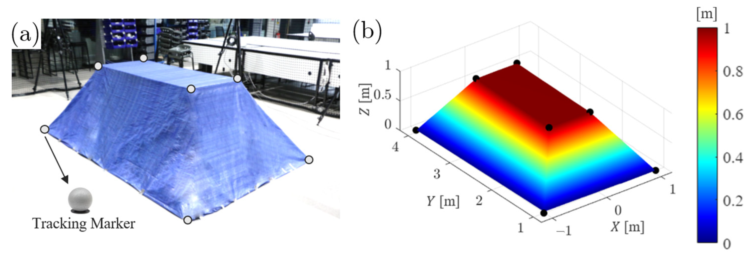
3.3. Reference Stockpile

The stockpile used in the current work as a demonstrative sample for evaluating our scanning approaches is the trapezoidal prism stockpile shown in Figure 8a. This shape has been chosen so that the actual volume can be determined easily using a precise measurement method, providing a basis for comparison and validation. Moreover, this stockpile shape is representative of stockpile shapes being typically considered in the literature [14,47]. We marked the shape’s corners with markers, as shown in Figure 8a, and acquired measurements directly from the motion tracking system. This is besides using additional testing with a 1D LiDAR mounted on a stick to collect dense data for the stockpile. The reconstructed surface is presented in Figure 8b, where the stockpile volume evaluation was 3 m³.

3.4. Data Collection

For the multi-drone experiments conducted, our reference stockpile was scanned using either two or three drones in formation leveraging the multi-agent adaptive formation control system. Figure 9 illustrates the scanning direction, desired waypoints, ${\mathit{W}}_k$, and formation shapes, ${\mathit{H}}_k$, at each waypoint. While the trajectory adopted here is not optimized for specific objective(s), it provides a uniform full coverage of the desired area without overlapping, similar to laying out a grid with a specific distance $s$, ensuring that all grid intersections are covered. The waypoints were placed at the corners of the area, while the formation shapes were designed to be a function of the drone number $m$ and the width of the area, denoted as $W$ in the figure. The formation shapes, as shown in the figure, are defined as follows:

$${\mathit{H}}_{1,i}=\left[s·(i-1),0)\right] \mathrm{for} i\in \left\{1,2,\dots ,m\right\},$$

(15)

$${\mathit{H}}_{2,i}=\left[s·(i-1),-s·(i-1)\right] \mathrm{for} i\in \left\{1,2,\dots ,m\right\},$$

(16)

$${\mathit{H}}_{3,i}=\left[-s·(i-1),-s·(i-1)\right] \mathrm{for} i\in \left\{1,2,\dots ,m\right\},$$

(17)

$${\mathit{H}}_{4,i}=\left[-s·(i-1),0)\right] \mathrm{for} i\in \left\{1,2,\dots ,m\right\},$$

(18)

$$s={\displaystyle \raisebox{1ex}{$W$}\!\left/ \!\raisebox{-1ex}{$(2m-1)$}\right.}$$

(19)

For the single-drone approach with a static 1D LiDAR, the drone was programmed to traverse a zigzag path over the stockpiles, almost covering the same grid with the specified distance $s$. This decision was intentional to ensure that the single-drone approach is using the closest possible trajectory to the multi-drone approach, hence ensuring a fair comparative analysis. While this trajectory choice is expected to lead to similar coverage when generating the point clouds from both approaches, this will also have consequences on other mission metrics, e.g., mission duration, which will be discussed later. Figure 10a and Figure 10c show the desired trajectories for using swarms of two and three drones, respectively, while Figure 10b,d show the closest possible comparable trajectories when applying a single drone using zigzag paths. That said, for the single-drone approach with the actuated 1D LiDAR, only four points at the corners of the area are set as waypoints (Figure 10e) due to the superior scanning coverage, obtained from actuation, when compared to the other approaches.

In conducting this data collection exercise, we chose two distinct altitudes for the drone flights: 1.5 m and 2 m. This decision was informed by the peak height of the stockpile, which was just below 1 m (i.e., 0.92 m). Lastly, and as explained previously, we ensured safety and precision during the indoor scans by capping the maximum drone speed to 0.1 m/s. This precaution ensured safe and controlled scanning within the confined indoor environment, minimising potential risks while optimising data accuracy. While the drones are set to fly in straight lines, at low speeds or due to wind disturbances, some oscillations and trim variations are expected. To address this, the 3D transformation matrix described in Section 2.5 registers the LiDAR data from the drone frame to the ground frame by incorporating the drone’s position and orientation in space. This approach compensates for any deviations from ideal rectilinear motion.

4. Results and Discussion

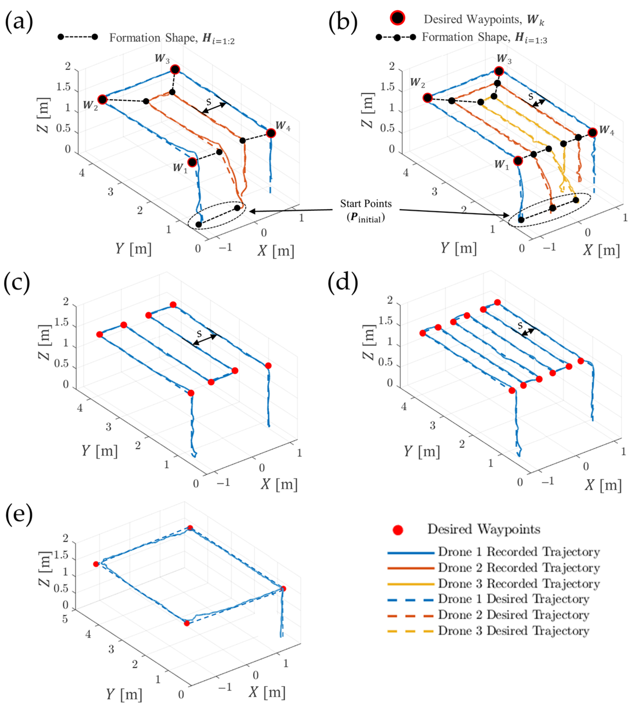
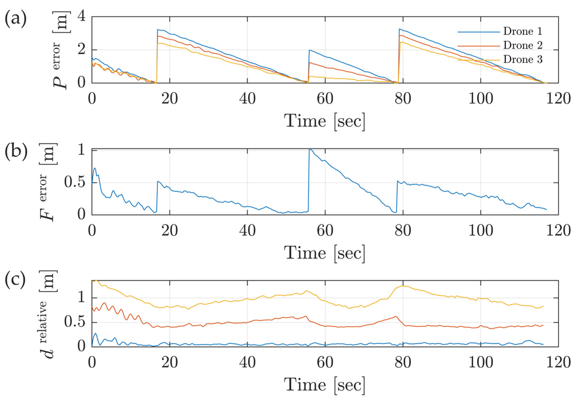
4.1. Flight Test Performance

In this subsection, we present the actual flight trajectories achieved, demonstrating the successful execution of the flight missions. Figure 11 illustrates the desired and recorded real 3D flight paths, confirming that the tracking system, communication setup, and control codes functioned as required. These drones initiated their flight with a take-off, performed the scanning mission at an altitude of 1.5 m, and completed the process with a successful landing. To demonstrate the new adaptive formation control algorithm proposed in this paper, Supplementary Videos (Videos S1 and S2) are provided, demonstrating two/three drones whilst conducting their scanning missions.

Due to the complexity of flying multiple drones in a simultaneous fashion, three distinct metrics were employed to assess the formation performance (as discussed previously): the positional error metric $\left(P_i^{\mathrm{error}}\left(t\right)\right)$, which measures the difference between drone $i$’s current and target positions at time $t$; the formation error metric ($F^{\mathrm{error}}\left(t\right)$), which evaluates the formation shape over time by comparing the current inter-drone distances with those of the desired formation at the next waypoint; and the relative distance ($d^{\mathrm{relative}}(t)$), between each drone’s current position ($P_i\left(t\right)$) and the desired position of drone 1 at a time $t$ within the planned trajectory. Figure 12 presents these metrics for the case shown in Figure 11b, exhibiting a notable pattern in the first two metrics where a surge in formation error—occurring during transitions in formation shape—gradually tapers as the drones advance towards the waypoint. This pattern of spike-and-decay in the error graph indicates the system’s ability to minimise both trajectory and formation errors simultaneously. Moreover, the third metric ($d^{\mathrm{relative}}\left(t\right)$) shows consistency and smooth transitions between different formation shapes.

Figure 13 shows the positional error $\left(P_i^{\mathrm{error}}\right(t\left)\right)$ for the single-drone approaches, demonstrating the difference between the drone’s current position and the next desired waypoint. Note that Figure 13a represents the case shown in Figure 11d for a single drone following a zigzag path, whereas Figure 13b represents the case shown in Figure 11e for a single drone equipped with the actuated 1D LiDAR.

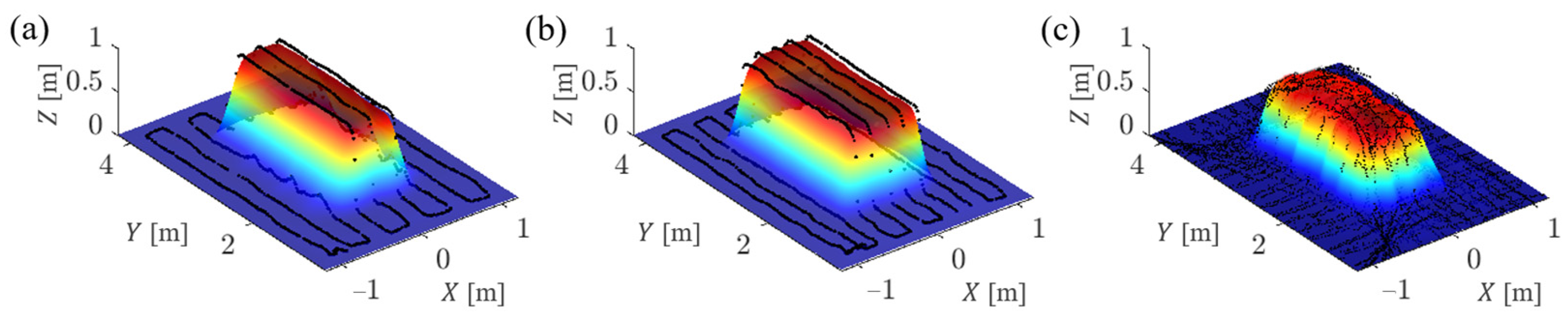
4.2. Point Cloud Registration and Stockpile Reconstruction

The visualisation of the point cloud registration and the 3D reconstructions are shown in Figure 14 for the reference stockpile shown in Figure 8a obtained through the various approaches considered: (a) two drones in formation, (b) three drones in formation, (c) a single drone navigating a conventional zigzag path, (d) a single drone following a denser zigzag path, and (e) a single drone equipped with the actuated 1D LiDAR system. The black scatters in the figure illustrate the point clouds ($\mathit{P}{\mathit{C}}_G$) obtained from the LiDAR data transformed into the global frame, and the 3D reconstructed surfaces are obtained from these registered point clouds. As expected, the employed drones with static 1D LiDAR, either operating alone or in formation, generated comparable point clouds, as indicated by the reconstructed surfaces in Figure 14a–d. The employed drones with static 1D LiDAR, either operating alone or in formation, generated comparable point clouds. That said, the employment of a drone equipped with an actuated LiDAR not only increased the density of the data captured but also fostered a comprehensive visualisation of the point cloud.

Next, we explore the volume estimation error. The estimated volumes obtained from the different drone approaches investigated, measured in cubic meters (m³), and their respective deviation errors as percentages from the evaluated reference volume are presented in

Table 1. Comparison of the reconstructed volumes and error values compared to the reference volume from the stockpiles mapping approaches considered in this study.

Methods	Altitude at 1.5 m		Altitude at 2.0 m
	Volume [m3]	Error [%]	Volume [m3]	Error [%]
Multi-Drone (2 Drones)	3.03	1.0	3.08	2.7
Multi-Drone (3 Drones)	3.01	0.3	3.04	1.3
Single Drone (Zigzag Path)	3.05	1.7	3.08	2.7
Single Drone (Finer Zigzag Path)	2.98	−0.7	3.03	1.0
Single Drone (Actuated 1D LiDAR)	3.11	3.7	3.15	5.0
Reference Volume [m3]	3.0

. The deviation percentage error is calculated from:

$$\mathrm{Error} [\%]={\displaystyle \frac{\mathrm{Estimated} \mathrm{Volume}-\mathrm{Reference} \mathrm{Volume}}{\mathrm{Reference} \mathrm{Volume}}}\times 100$$

(20)

The results illustrate that the approaches leveraging a formation of two or three drones, or a single drone following zigzag paths, can generate a promising average volumetric error margin of 1.6%. That said, the conducted tests using the two drones, and the first zigzag path led to a slightly higher estimated volume, hence a larger error, in comparison with the conducted tests using three drones and the second zigzag path. It is expected that employing a finer trajectory and/or increasing the number of drone agents within the formation will allow better coverage and increase the density of the point clouds registered. This, in turn, is expected to improve the estimation of the volume, particularly when considering more irregular stockpile shapes. That said, there can be a limit to the improvement achieved as a much denser point cloud does not always guarantee better outcomes. This is, in fact, demonstrated here from the servo-actuated 1D LiDAR approach, which displayed the highest volumetric error rate of 4.7%. This is mainly due to the generation of a point cloud with a significant number of outlier points and common LiDAR bias when scanning at non-vertical angles [48], as illustrated in Figure 14e, which led to the overestimated volume, and the highest volumetric error percentage.

Our findings also reveal that increasing the altitude from 1.5 m to 2.0 m led to an increase in the estimated volume. This slight inflation is mainly attributed to object detection occurring further away from the centre of the Field of View (FOV), as illustrated in Figure 15. Therefore, future implementation of a narrower FOV sensor could potentially enhance the accuracy. That said, for larger objects, the effect of false recorded ranges shown in Figure 15 becomes less significant compared to the object size. Additionally, there is a tendency for increased volumetric errors when estimating the volumes of smaller piles, as discussed in [13].

4.3. Comparative Analysis with a Second Object: Rectangular Prism Stockpile

In addition to the previously scanned stockpile, an additional scanning mission was conducted on a second reference object with a rectangular prism shape, as shown in Figure 16a. This object was chosen to provide a contrasting geometry to the trapezoidal prism tested earlier. Given its smaller size and sharper edges, this experiment aimed to assess the impact of scanning such challenging objects on our method which relies on a low-cost 1D LiDAR and inherently produces less detailed point clouds. Similar to the first object, the corners were marked with tracking markers, and ground-truth measurements were acquired directly from the motion-tracking system. The reconstructed surface of the rectangular prism stockpile is presented in Figure 16b, with an evaluated volume of 1.33 m³.

For this stockpile, it was not feasible to use the multi-drone approach due to the relatively small size of the object, as it has a top-projected area of 1.8 m × 0.8 m. Instead, the following single-drone approaches were tested: (a) a drone following a zigzag path with a 0.25 m line gap, (b) a drone following a denser zigzag path with a 0.20 m line gap, and (c) a drone equipped with an actuated 1D LiDAR system. All tests were conducted at a 1.5 m altitude, and the point cloud registration and 3D reconstructions obtained through each approach are illustrated in Figure 17.

The estimated volumes obtained from the different single-drone approaches investigated along with their respective volumetric errors were 1.64 m³ for the zigzag path (23% volumetric error), 1.87 m³ for the denser zigzag path (40% volumetric error), and 1.71 m³ for the actuated 1D LiDAR system (28% volumetric error). Remarkably, the approaches that provide a more refined reconstruction of the shape also resulted in higher volumetric error. These higher estimated volumetric errors are likely due to the challenges associated with reconstructing the sharp edges of the rectangular box shape, which can potentially add extra volume, and the tendency for increased volumetric errors when estimating the volumes of smaller piles, as discussed earlier. Moreover, the FOV of the ToF sensor leads to object detection occurring further away from the centre, as shown in Figure 18. The amount of outliers around the sharp edges is relatively large compared to the object size, which could lead to a smaller volumetric error when scanning larger objects. This aligns with previous studies [49,50,51], which have shown that LiDAR-based volume estimations are more prone to errors when scanning smaller objects with sharp edges due to point cloud sparsity and interpolation challenges.

4.4. Comparative Analysis of the Proposed Approaches

There is a close resemblance between the stockpile volume estimation figures obtained from the multi-drone scanning and those from the single drone when following analogous zigzag trajectories. This is expected as the same drone and sensor, and almost the same trajectory, were used in these experiments. In fact, the small difference in the shape of the trajectory (between the multi- and single-drone experiments; see Figure 10) is the main cause for the small difference in the obtained stockpile volume estimates. That said, when comparing these approaches, there are other metrics to consider including the mission duration and cost. As shown in Figure 10, when illustrating the desired trajectories for each approach, in the multi-drone system, the longest distance was for drone 1 measuring 8 m (hence, for our set maximum velocity value, this means a flight duration of around 80 s). This distance remained consistent whether two or three drones were used. However, when applying the single drone with zigzag trajectories, the trajectory distance increased to 14 m (around 140 s), and further to 20 m (around 200 s) when using a finer zigzag path. When using the single drone with the actuated 1D LiDAR, the desired distance was 10 m (around 100 s). Clearly, the multi-drone approach leads to shorter mission durations, compared to the single-drone approaches which need longer trajectories and hence flight time to complete the mission. Note that the Crazyflie 2.1 drone has around seven minutes of maximum flight time. Therefore, in other scenarios, this may dictate the need for a larger battery and hence a larger drone to complete the mission.

On the other hand, the initial investment cost in a multi-drone approach is higher, with the cost increasing as the number of agents increases. In the case of this work, a single Crazyflie 2.1 with the flow deck costs around GBP 220, while the Parrot drone with the actuated 1D LiDAR system costs around GBP 500 (prices based on 2023 UK market figures). Note that the number of agents within a system will depend on the targeted scanning accuracy required for a given area to be inspected. That said, if the system is intended for frequent use, then this initial investment becomes more justified. However, it is infeasible to estimate the exact time required to amortise this initial investment, as it depends on factors such as usage frequency, operational costs, and specific inspection demands. Finally, the multi-drone approach also offers the unique benefit of redundancy, i.e., if one agent fails to complete the mission, then the other drones can be reconfigured to accomplish the scanning mission. This is attractive for scanning missions in unknown spaces, particularly where the chances of collision with various obstacles are high.

All in all, the choice to use any of the approaches presented is a user decision based on several factors, including location, time, and cost constraints. To facilitate this decision,

Table 2. Comparison of the advantages and disadvantages of the three main existing stockpile mapping techniques.

Approaches	Advantages	Disadvantages
Multi-drone agents with static 1D LiDAR	Fast scanning	High initial cost
	Applicable using micro drones	Coordination complexity
	Provides redundancy	Point cloud resolution relies on the number of agents
Single drone with static 1D LiDAR	Low initial cost	Slow scanning
	Applicable using micro drones	May require larger battery or mid-operation replacement
	Ease of operation	Point cloud resolution relies on the number of trajectory waypoints
Single drone with an actuated 1D LiDAR	Fast scanning	Data outliers and noise
	Enriched point cloud	Mechanical complexity
	Enhanced scanning of angles

presents a comparative analysis highlighting the main advantages and disadvantages of the three tested stockpile volume estimation methods presented in this paper.

5. Final Comments

5.1. Outcomes

In this study, we aimed to assess and compare the accuracy and efficacy of employing different drone-based approaches that employ low-cost 1D-LiDAR scanning sensors for point cloud registration and stockpile reconstruction. Our key accomplishments can be outlined as follows:

• A new adaptive formation control approach was developed for drone formation and trajectory tracking, ensuring smooth transitions between formation shapes by dynamically adjusting the drones’ velocities;
• Experimental tests were performed to scan an example stockpile within an indoor environment using multi-drone systems consisting of Crazyflie micro drones, demonstrating successful deployment of the proposed formation algorithm in a real experimental test, achieving an average deviation of 0.23% between the desired and actual paths of each drone within the formation;
• In comparison, the stockpile was also scanned using a solitary drone with either a static or actuated 1D LiDAR (with the latter approach being previously proposed based on simulation assessments, but we experimentally demonstrate its efficacy in this work);
• Successful approach integration was achieved through the development of Python codes to control the drones, seamlessly merging the data of the motion tracking system through ROS communication, and the developed codes have been provided in Supplementary Materials, Code S1;
• In terms of volumetric estimation of the reference trapezoidal prism stockpile considered in this study, whilst using the Crazyflie micro drones, a formation of two or three drones, or a single drone following closely similar zigzag paths, generated similar results with a promising average volumetric error margin of 1.3%. On the other hand, the servo-actuated 1D LiDAR approach showed a higher volumetric average error rate of 4.4% due to the significant number of outlier points and common LiDAR bias when scanning at non-vertical angles;
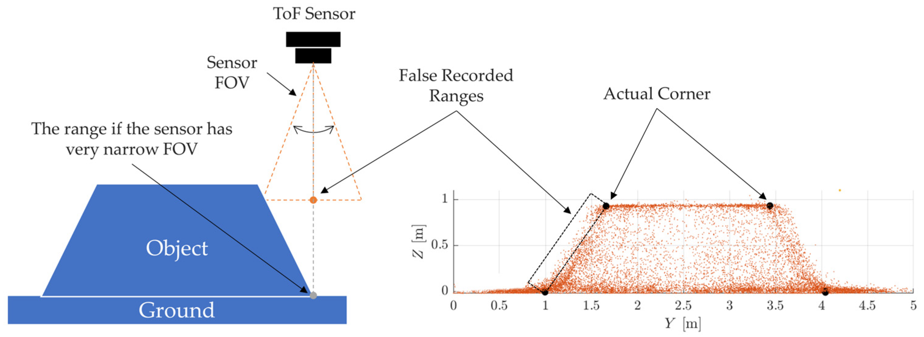
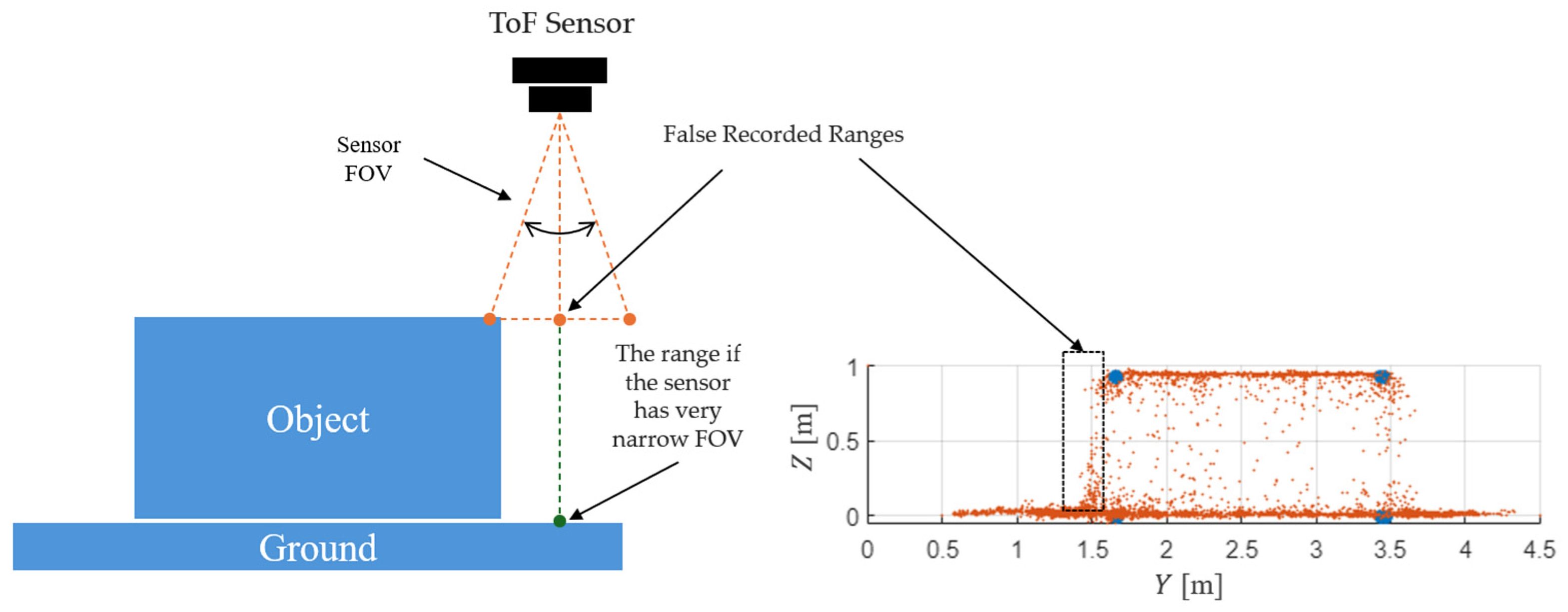
• For the second scanned shape, a smaller rectangular prism, the volumetric error increased dramatically due to challenges in reconstructing sharp edges and the impact of the ToF sensor’s FOV on object detection;
• In terms of flight time, the multi-drone approach and the single drone with the actuated 1D LiDAR approach significantly reduce mission duration compared to a single drone with a static sensor following a zigzag pattern trajectory. While deploying multiple drones increases the initial investment cost, it provides redundancy to the system and is beneficial in scenarios where a larger area needs to be scanned, which a single drone is expected not to be able to fully cover due to battery limitations. Meanwhile, the single drone with the actuated 1D LiDAR approach seems to offer a balance between flight time and cost. However, it has some limitations, such as mechanical complexity, data outliers, and noise, which lead to an increase in the estimated volumetric error.

5.2. Future Work

Future research directions that we believe will further refine the current methodologies and expand the scope of this research include the following:

• Develop an automated approach for waypoints and formation topologies selection to provide an optimised coverage of the desired area;
• Investigate adaptive path optimization techniques for the multi-agent system, particularly for larger stockpile areas, to improve efficiency while maintaining coordinated flight and uniform coverage;
• Test the proposed multi-drone approach in conjunction with the dynamic formation strategy in large stockpile storages, where active collision avoidance would be essential;
• Integrate a leader–follower multi-agent system, providing the leader drone with enhanced capabilities, such as obstacle detection, and facilitating real-time information sharing with follower drones to further optimise operations;
• Integrate narrow FOV sensors within micro drones, as this would promise more accurate data acquisition by minimising errors and enhancing the fine details reconstruction.

References

1. Hassanalian, M.; Rice, D.; Abdelkefi, A. Evolution of Space Drones for Planetary Exploration: A Review. Progress Aerosp. Sci. 2018, 97, 61–105. [Google Scholar] [CrossRef]
2. Bayomi, N.; Fernandez, J.E.; Bayomi, N.; Fernandez, J.E. Eyes in the Sky: Drones Applications in the Built Environment under Climate Change Challenges. Drones 2023, 7, 637. [Google Scholar] [CrossRef]
3. Zhang, J.; Zhao, N.; Qu, F. Bio-Inspired Flapping Wing Robots with Foldable or Deformable Wings: A Review. Bioinspir Biomim. 2022, 18, 011002. [Google Scholar] [CrossRef]
4. Ducard, G.J.J.; Allenspach, M. Review of Designs and Flight Control Techniques of Hybrid and Convertible VTOL UAVs. Aerosp. Sci. Technol. 2021, 118, 107035. [Google Scholar] [CrossRef]
5. Phan, H.V.; Park, H.C. Insect-Inspired, Tailless, Hover-Capable Flapping-Wing Robots: Recent Progress, Challenges, and Future Directions. Progress Aerosp. Sci. 2019, 111, 100573. [Google Scholar] [CrossRef]
6. Shearwood, T.R.; Nabawy, M.R.A.; Crowther, W.J.; Warsop, C. A Novel Control Allocation Method for Yaw Control of Tailless Aircraft. Aerospace 2020, 7, 150. [Google Scholar] [CrossRef]
7. Shearwood, T.R.; Nabawy, M.R.; Crowther, W.J.; Warsop, C. Directional Control of Finless Flying Wing Vehicles—An Assessment of Opportunities for Fluidic Actuation. In Proceedings of the AIAA Aviation 2019 Forum; American Institute of Aeronautics and Astronautics: Reston, Virginia, 2019. [Google Scholar]
8. Shearwood, T.R.; Nabawy, M.R.A.; Crowther, W.J.; Warsop, C. Coordinated Roll Control of Conformal Finless Flying Wing Aircraft. IEEE Access 2023, 11, 61401–61411. [Google Scholar] [CrossRef]
9. Lanteigne, E.; Alsayed, A.; Robillard, D.; Recoskie, S.G. Modeling and Control of an Unmanned Airship with Sliding Ballast. J. Intell. Robot. Syst. 2017, 88, 285–297. [Google Scholar] [CrossRef]
10. Näsi, R.; Mikkola, H.; Honkavaara, E.; Koivumäki, N.; Oliveira, R.A.; Peltonen-Sainio, P.; Keijälä, N.-S.; Änäkkälä, M.; Arkkola, L.; Alakukku, L. Can Basic Soil Quality Indicators and Topography Explain the Spatial Variability in Agricultural Fields Observed from Drone Orthomosaics? Agronomy 2023, 13, 669. [Google Scholar] [CrossRef]
11. Korpela, I.; Polvivaara, A.; Hovi, A.; Junttila, S.; Holopainen, M. Influence of Phenology on Waveform Features in Deciduous and Coniferous Trees in Airborne LiDAR. Remote Sens. Environ. 2023, 293, 113618. [Google Scholar] [CrossRef]
12. Sliusar, N.; Filkin, T.; Huber-Humer, M.; Ritzkowski, M. Drone Technology in Municipal Solid Waste Management and Landfilling: A Comprehensive Review. Waste Manag. 2022, 139, 1–16. [Google Scholar] [CrossRef] [PubMed]
13. Alsayed, A.; Nabawy, M.R.A. Stockpile Volume Estimation in Open and Confined Environments: A Review. Drones 2023, 7, 537. [Google Scholar] [CrossRef]
14. Tucci, G.; Gebbia, A.; Conti, A.; Fiorini, L.; Lubello, C. Monitoring and Computation of the Volumes of Stockpiles of Bulk Material by Means of UAV Photogrammetric Surveying. Remote Sens. 2019, 11, 1471. [Google Scholar] [CrossRef]
15. Ajayi, O.G.; Ajulo, J. Investigating the Applicability of Unmanned Aerial Vehicles (UAV) Photogrammetry for the Estimation of the Volume of Stockpiles. Quaest. Geogr. 2021, 40, 25–38. [Google Scholar] [CrossRef]
16. Tamin, M.A.; Darwin, N.; Majid, Z.; Mohd Ariff, M.F.; Idris, K.M.; Manan Samad, A. Volume Estimation of Stockpile Using Unmanned Aerial Vehicle. In Proceedings of the 2019 9th IEEE International Conference on Control System, Computing and Engineering (ICCSCE), Penang, Malaysia, 29 November–1 December 2019; pp. 49–54. [Google Scholar]
17. Alsayed, A.; Yunusa-Kaltungo, A.; Quinn, M.K.; Arvin, F.; Nabawy, M.R.A. Drone-Assisted Confined Space Inspection and Stockpile Volume Estimation. Remote Sens. 2021, 13, 3356. [Google Scholar] [CrossRef]
18. Dang, T.; Tranzatto, M.; Khattak, S.; Mascarich, F.; Alexis, K.; Hutter, M. Graph-Based Subterranean Exploration Path Planning Using Aerial and Legged Robots. J. Field Robot. 2020, 37, 1363–1388. [Google Scholar] [CrossRef]
19. Cao, D.; Zhang, B.; Zhang, X.; Yin, L.; Man, X. Optimization Methods on Dynamic Monitoring of Mineral Reserves for Open Pit Mine Based on UAV Oblique Photogrammetry. Measurement 2023, 207, 112364. [Google Scholar] [CrossRef]
20. Bircher, A.; Kamel, M.; Alexis, K.; Oleynikova, H.; Siegwart, R. Receding Horizon Path Planning for 3D Exploration and Surface Inspection. Auton. Robot. 2018, 42, 291–306. [Google Scholar] [CrossRef]
21. Yin, H.; Tan, C.; Zhang, W.; Cao, C.; Xu, X.; Wang, J.; Chen, J. Rapid Compaction Monitoring and Quality Control of Embankment Dam Construction Based on UAV Photogrammetry Technology: A Case Study. Remote Sens. 2023, 15, 1083. [Google Scholar] [CrossRef]
22. Salagean, T.; Suba, E.; Pop, I.D.; Matei, F.; Deak, J. Determining Stockpile Volumes Using Photogrammetric Methods. Sci. Papers Ser. E Land Reclam. Earth Obs. Surv. Environ. Eng. 2019, 8, 114–119. [Google Scholar]
23. Rhodes, R.K. UAS as an Inventory Tool: A Photogrammetric Approach to Volume Estimation; University of Arkansas: Fayetteville, AR, USA, 2017. [Google Scholar]
24. Eisenbeiss, H. UAV Photogrammetry. Ph.D. Thesis, Institut für Geodesie und Photogrammetrie, Zürich, Switzerland, 2009. [Google Scholar]
25. Kokamägi, K.; Türk, K.; Liba, N. UAV Photogrammetry for Volume Calculations. Agron. Res. 2020, 18, 2087–2102. [Google Scholar] [CrossRef]
26. Vacca, G. UAV Photogrammetry for Volume Calculations. A Case Study of an Open Sand Quarry. In Computational Science and Its Applications—ICCSA 2022 Workshops; Springer: Cham, Switzerland, 2022; Volume 13382, pp. 505–518. [Google Scholar] [CrossRef]
27. Cho, S.I.; Lim, J.H.; Lim, S.B.; Yun, H.C. A Study on DEM-Based Automatic Calculation of Earthwork Volume for BIM Application. J. Korean Soc. Surv. Geod. Photogramm. Cartogr. 2020, 38, 131–140. [Google Scholar] [CrossRef]
28. Rohizan, M.H.; Ibrahim, A.H.; Abidin, C.Z.C.; Ridwan, F.M.; Ishak, R. Application of Photogrammetry Technique for Quarry Stockpile Estimation. IOP Conf. Ser. Earth Environ. Sci. 2021, 920, 012040. [Google Scholar] [CrossRef]
29. Zhang, L.; Grift, T.E. A LIDAR-Based Crop Height Measurement System for Miscanthus Giganteus. Comput. Electron. Agric. 2012, 85, 70–76. [Google Scholar] [CrossRef]
30. Carabassa, V.; Montero, P.; Alcañiz, J.M.; Padró, J.-C. Soil Erosion Monitoring in Quarry Restoration Using Drones. Minerals 2021, 11, 949. [Google Scholar] [CrossRef]
31. Forte, M.; Neto, P.; Thé, G.; Nogueira, F. Altitude Correction of an UAV Assisted by Point Cloud Registration of LiDAR Scans. In Proceedings of the 18th International Conference on Informatics in Control, Automation and Robotics, Virstual, 6–8 July 2021; SCITEPRESS—Science and Technology Publications: Setúbal, Portugal, 2021; pp. 485–492. [Google Scholar]
32. Bayar, G. Increasing Measurement Accuracy of a Chickpea Pile Weight Estimation Tool Using Moore-Neighbor Tracing Algorithm in Sphericity Calculation. J. Food Meas. Charact. 2021, 15, 296–308. [Google Scholar] [CrossRef]
33. Phillips, T.G.; Guenther, N.; McAree, P.R. When the Dust Settles: The Four Behaviors of LiDAR in the Presence of Fine Airborne Particulates. J. Field Robot 2017, 34, 985–1009. [Google Scholar] [CrossRef]
34. Alsayed, A.; Nabawy, M.R.A. Indoor Stockpile Reconstruction Using Drone-Borne Actuated Single-Point LiDARs. Drones 2022, 6, 386. [Google Scholar] [CrossRef]
35. Amaglo, W.Y. Volume Calculation Based on LiDAR Data. Master's Thesis, Royal Institute of Technology, Stockholm, Sweden, 2021. [Google Scholar]
36. Zhang, W.; Yang, D. Lidar-Based Fast 3D Stockpile Modeling. In Proceedings of the 2019 International Conference on Intelligent Computing, Automation and Systems (ICICAS), Chongqing, China, 6–8 December 2019; pp. 703–707. [Google Scholar]
37. Flyability Elios 3—Digitizing the Inaccessible. Available online: https://www.flyability.com/elios-3 (accessed on 22 August 2022).
38. Alsayed, A.; Nabawy, M.R.; Arvin, F. Autonomous Aerial Mapping Using a Swarm of Unmanned Aerial Vehicles. In Proceedings of the AIAA AVIATION 2022 Forum; American Institute of Aeronautics and Astronautics: Reston, Virginia, 2022. [Google Scholar]
39. Raj, T.; Hashim, F.H.; Huddin, A.B.; Ibrahim, M.F.; Hussain, A. A Survey on LiDAR Scanning Mechanisms. Electronics 2020, 9, 741. [Google Scholar] [CrossRef]
40. Vicon|Award Winning Motion Capture Systems. Available online: https://www.vicon.com/ (accessed on 12 September 2023).
41. Home|Bitcraze. Available online: https://www.bitcraze.io/ (accessed on 12 September 2023).
42. Flow Deck v2|Bitcraze. Available online: https://www.bitcraze.io/products/flow-deck-v2/ (accessed on 9 July 2024).
43. Kilberg, B.G.; Campos, F.M.R.; Schindler, C.B.; Pister, K.S.J. Quadrotor-Based Lighthouse Localization with Time-Synchronized Wireless Sensor Nodes and Bearing-Only Measurements. Sensors 2020, 20, 3888. [Google Scholar] [CrossRef]
44. Vicon_Bridge—ROS Wiki. Available online: http://wiki.ros.org/vicon_bridge (accessed on 12 September 2023).
45. GitHub—Bitcraze/Crazyflie-Lib-Python: Python Library to Communicate with Crazyflie. Available online: https://github.com/bitcraze/crazyflie-lib-python/tree/master (accessed on 12 September 2023).
46. Pyparrot Documentation. Available online: https://pyparrot.readthedocs.io/en/latest/index.html (accessed on 12 September 2023).
47. He, H.; Chen, T.; Zeng, H.; Huang, S. Ground Control Point-Free Unmanned Aerial Vehicle-Based Photogrammetry for Volume Estimation of Stockpiles Carried on Barges. Sensors 2019, 19, 3534. [Google Scholar] [CrossRef] [PubMed]
48. Aziz, F.N.; Zakarijah, M. TF-Mini LiDAR Sensor Performance Analysis for Distance Measurement. J. Nas. Tek. Elektro Dan Teknol. Inf. 2022, 11, EN-192–EN-198. [Google Scholar]
49. Petras, V.; Petrasova, A.; McCarter, J.B.; Mitasova, H.; Meentemeyer, R.K. Point Density Variations in Airborne Lidar Point Clouds. Sensors 2023, 23, 1593. [Google Scholar] [CrossRef]
50. Alaba, S.Y.; Ball, J.E. A Survey on Deep-Learning-Based LiDAR 3D Object Detection for Autonomous Driving. Sensors 2022, 22, 9577. [Google Scholar] [CrossRef]
51. You, J.; Kim, Y.-K. Up-Sampling Method for Low-Resolution LiDAR Point Cloud to Enhance 3D Object Detection in an Autonomous Driving Environment. Sensors 2022, 23, 322. [Google Scholar] [CrossRef]
Figure 1. (a) Paths of the three drones starting from origin, illustrating formation transitions between waypoints. (b) Position error, P error , over time for each drone, showing synchronised arrivals at waypoints. (c) Reduction in formation error, F error , as the drones get nearer to the waypoints. (d) Relative position, d i relative , between each drone’s current position and the desired position of drone 1 over time, demonstrating the algorithm’s ability to maintain consistent formations during transitions.
Aerospace 12 00189 g001
Figure 2. A schematic illustration of the actuated 1D LiDAR approach.
Aerospace 12 00189 g002
Figure 3. A schematic illustration of a single drone with a static 1D LiDAR following a zigzag trajectory.
Aerospace 12 00189 g003
Figure 4. Views of the netted drone flight test enclosure. Highlighted are the advanced VICON motion tracking system components. The inset image also showcases the Crazyflie 2.1 drone in action while above the blue stockpile.
Aerospace 12 00189 g004
Figure 5. Crazyflie 2.1 drones equipped with four, one large and three smaller, markers for accurate tracking during the experiments.
Aerospace 12 00189 g005
Figure 6. A schematic setup showcasing the connectivity between the VICON cameras, the main PC, and the ground station laptop facilitating real-time tracking and communication with the drones.
Aerospace 12 00189 g006
Figure 7. Illustration of the actuated 1D LiDAR setup, showcasing the integration of a Raspberry Pi and TFMini LiDAR sensor mounted on a servo motor, all attached to a Parrot Bebop 2 drone, equipped with markers for motion tracking. The figure includes a schematic representation for clearer visualisation of the actuated 1D LiDAR system.
Aerospace 12 00189 g007
Figure 8. (a) The reference stockpile used for scanning demonstrations of the proposed approaches, highlighting the corner points hosting the markers to determine the actual volume. (b) Visualisation of the 3D reconstruction of the reference stockpile shape with the shape’s corners being represented as black dots. The colour gradient indicates height variations.
Aerospace 12 00189 g008
Figure 9. Desired waypoints W k , denoted as red circles, and the corresponding formation shapes H k , showcasing the cooperation of waypoints and formation shapes in ensuring comprehensive, non-overlapping coverage of all the desired area.
Aerospace 12 00189 g009
Figure 10. Desired trajectories for each applied approach. (a) The desired trajectories for the multi-agent system with two drones, and (b) a comparative trajectory to (a) when using a single drone. (c) The desired trajectories for the multi-agent system with three drones, and (d) a comparative trajectory to (c) when using a single drone. (e) The trajectory for a single drone with an actuated 1D LiDAR. The points A1–A4, B1–B4, and C1–C4 represent the waypoints for Drone 1, Drone 2, and Drone 3, respectively.
Aerospace 12 00189 g010
Figure 11. Illustration of the 3D desired and actual recorded trajectories for (a) two and (b) three drones trajectories in formation, (c) a zigzag trajectory of a single drone loosely similar to the two drones in formation, (d) a finer zigzag trajectory of a single drone analogous to that of three drones in formation, and (e) the recorded simple trajectory for the single drone equipped with the actuated 1D LiDAR. The mission includes phases of take-off, scanning at a 1.5 m altitude, and landing. Moreover, (a,b) demonstrate the predefined formation shapes ( H k ) at desired waypoints ( W k ). The distances s in (a,b) are obtained using Equation (18), and then used to design the zigzag path shown in (c,d).
Aerospace 12 00189 g011
Figure 12. Performance metrics for the formation system based on experimental measurements, illustrating the simultaneous reduction in both trajectory error ( P error ) and formation error ( F error ) as shown in (a,b), respectively; and consistency between different formation shapes as shown by the metric d   relative in (c).
Aerospace 12 00189 g012
Figure 13. Performance of the system’s ability to minimise trajectory error for the single-drone approaches with (a) a static LiDAR shown in Figure 11d, and (b) actuated 1D LiDAR shown in Figure 11e.
Aerospace 12 00189 g013
Figure 14. Illustration of the registered point clouds ( P C G ), shown in black scatters, and the 3D reconstructed shapes, shown in colour gradient, for the stockpile displayed in Figure 8a, while employing (a) two drones in formation, (b) three drones in formation, (c) a single drone navigating a zigzag path, (d) a single drone following a denser zigzag path, and (e) a solitary drone equipped with the actuated 1D LiDAR system. The colour gradient indicates varying heights.
Aerospace 12 00189 g014
Figure 15. A schematic representation highlighting potential inaccuracies in point cloud collection owing to having a wider FOV sensor, which tends to capture the closest data point. The point cloud shown in this figure was obtained using additional testing with a 1D LiDAR mounted on a stick to collect dense data.
Aerospace 12 00189 g015
Figure 16. (a) Second reference stockpile used for scanning demonstrations. (b) Visualisation of the 3D reconstruction of the reference stockpile shape with the shape’s corners being represented as black dots. The colour gradient indicates height variations.
Aerospace 12 00189 g016
Figure 17. Illustration of the registered point clouds ( P C G ), shown in black scatters, and the 3D reconstructed shapes, shown in colour gradient, for the stockpile displayed in Figure 16, while employing (a) a single drone navigating a zigzag path, (b) a single drone following a denser zigzag path, and (c) a solitary drone equipped with the actuated 1D LiDAR system. The colour gradient indicates varying heights.
Aerospace 12 00189 g017
Figure 18. A schematic representation highlighting potential inaccuracies in point cloud collection due to the use of a wider FOV sensor, which makes it difficult to reconstruct sharp edges, leading to an increase in the estimated volume. The blue dots show the actual shape corners from the side view.
Aerospace 12 00189 g018