Numerical Predictions of Low-Reynolds-Number Propeller Aeroacoustics: Comparison of Methods at Different Fidelity Levels ^†

Abstract

Low-Reynolds-number propeller systems have been widely used in aeronautical applications, such as unmanned aerial vehicles (UAV) and electric propulsion systems. However, the aerodynamic sound of the propeller systems is often significant and can lead to aircraft noise problems. Therefore, effective predictions of propeller noise are important for designing aircraft, and the different phases in aircraft design require specific prediction approaches. This paper aimed to perform a comparison study on numerical methods at different fidelity levels for predicting the aerodynamic noise of low-Reynolds-number propellers. The Ffowcs-Williams and Hawkings (FWH), Hanson, and Gutin methods were assessed as, respectively, high-, medium-, and low-fidelity noise models. And a coarse-grid large eddy simulation was performed to model the propeller aerodynamics and to inform the three noise models. A popular propeller configuration, which has been used in previous experimental and numerical studies on propeller noise, was employed. This configuration consisted of a two-bladed propeller mounted on a cylindrical nacelle. The propeller had a diameter of $D=9^{″}$ and a pitch-to-diameter ratio of $P/D=1$, and was operated in a forward-flight condition with a chord-based Reynolds number of $Re=4.8\times {10}^4$, a tip Mach number of $M=0.231$, and an advance ratio of $J=0.485$. The results were validated against existing experimental measurements. The propeller flow was characterized by significant tip vortices, weak separation over the leading edges of the blade suction sides, and small-scale vortical structures from the blade trailing edges. The far-field noise was characterized by tonal noise, as well as broadband noise. The mechanism of the noise generation and propagation were clarified. The capacities of the three noise modeling methods for predicting such propeller noise were evaluated and compared.

1. Introduction

Today’s aeronautical society is required to develop advanced aircraft configurations and technologies which lower overall emissions. Propeller propulsion systems have emerged as a promising technology for reducing the fuel consumption and emissions of future passenger aircraft as compared to conventional turbofan engines [1]. The advantage is owing to the high propulsive efficiency of propeller propulsion systems at moderate flight speeds [2], as well as their compatible implementations in trending electric aircraft [3]. Despite the potential benefits of propeller propulsion systems, aerodynamically generated noise remains a significant concern for this technology. Without noise-shielding nacelles, propeller-driven aircraft faces difficulties in meeting certification noise requirements [2]. Our focus is on the numerical prediction of the aerodynamic noise of low-Reynolds-number propellers, which are used on small-scale and low-speed aircraft.

The generation mechanism of propeller aerodynamic noise was theoretically reviewed in previous research [4], revealing that tonal noise with a discrete frequency is generated by air volume displacement, due to the rotational motion of propeller blades (i.e., thickness noise) and the phase displacement of blade aerodynamic loading (i.e., loading noise). On the other hand, noise with broadband frequency is generated by the fluctuating surface pressure resulting from turbulent flow over blades (i.e., trailing-edge noise) and quadruple noise sources, due to the turbulence itself (i.e., turbulence noise). Based on understanding of the generation mechanism, many models have been developed for predicting the aerodynamic noise of propellers and rotors [5,6,7]. Most conventional models are applied with deterministic noise sources [8], where the aerodynamics of propellers need to be known in advance. A semi-empirical model developed by Gutin [9] provides a simplified method for estimating propeller noise, considering factors such as thrust, power consumption, diameter, blade count, and tip Mach number. Gutin’s approach primarily focuses on the sound pressure produced by the propeller as a single source at the hub, and incorporates noise attenuation at higher harmonics using Bessel functions [9]. The good accuracy of Gutin’s method was reported at the first harmonic level for helicopters and propeller driven aircraft in static or low-forward-speed (below 40 knots) conditions [10]. However, broadband noise is considered to be insignificant and is neglected in this model, because the broadband noise induced by fluctuating pressure is not significant for propeller blades at low angles of attack, and the quadruple noise is also weak at low helical tip Mach numbers ($M<0.9$) [11]. Based on the same assumptions, Hanson proposed a model which focuses on the lift, drag, and volume displacement of each blade element and incorporates key parameters from Gutin’s work [12]. Hanson’s method computes sound pressure in the frequency domain through integration along the propeller radius using far-field equations, considering the Doppler effect, geometry effects (e.g., sweep and lean), and aeroacoustic non-compactness noise sources [13]. The good accuracy of Hanson’s method was reported as within 0.2 dB for the near- and the far-field of a 6-bladed propeller at a flight Mach number of 0.46 and a propeller tip rotational Mach number of 0.677 [14]. With advances in computational aeroacoustics (CAA), higher-fidelity modeling of the three-dimensional flow and noise generation of propellers with complicate geometries has been enabled [15]. Most CAA methods are performed in a hybrid way, where the propeller flow field is first solved, often by computational fluid dynamics (CFD), and then the acoustic field is computed by the methods of acoustic analogy, e.g., the Ffowcs-Williams and Hawkings (FWH) method [16]. Huang et al. performed large eddy simulations (LES) and the FWH method to predict the far-field noise, including the broadband noise, of a propeller–wing configuration and achieved a good agreement, within 1.42 dB [17]. In addition, the acoustic solution of flow passing propellers can be obtained simultaneously with a flow solution using direct aeroacoustic simulations, which solve the governing equations of compressible flow using high-accuracy algorithms [18,19].

For aircraft design, models at different fidelity levels are required [2]. For example, lower-fidelity and fast-predictive models are demanded for conceptional design. In contrast, higher-fidelity models are demanded for detailed design. Although multi-fidelity noise models for modeling propeller noise have been evaluated and compared in previous studies [20,21], similar comparison studies have not been conducted for low-Reynolds-number propellers. These propellers are generally operated at Reynolds numbers of $Re={10}^4-{10}^5$ and Mach numbers of $M\le 0.3$ [22]. The Reynolds number is defined based on the rotational velocity $V_{75}$ and the chord length $c_{75}$ at the 75% blade station, and the Mach number is defined based on the propeller tip velocity $V_{100}$ as

$$Re=V_{75}{c}_{75}/{\nu }_0,M=V_{100}/a_0$$

(1)

where ${\nu }_0$ denotes freestream kinetic viscosity and $a_0$ is sound speed. In contrast, the Reynolds number regime of traditional rotorcraft is higher and at $Re\ge {10}^6$ [22]. Previous research has shown that low-Reynolds-number propellers have different flow structures from traditional propellers and, hence, different noise generation mechanisms [22]. Therefore, it is worth investigating multi-fidelity methods as applied to modeling low-Reynolds-number propeller noise, to give perspectives for aircraft design.

A multi-fidelity framework for modeling aircraft noise has been developed in our recent works. In a previous paper [23], we demonstrated some successful implementations of modeling low-Reynolds-number propeller noise using three noise models at different fidelity levels. Noticeable differences were observed in the results of the three models [23]. In this paper, we aimed to extend the study by comprehensively comparing the capacities of three multi-fidelity noise models for predicting low-Reynolds-number propeller aeroacoustics. A benchmark propeller configuration was used as the demonstration case. This paper is outlined as follows. In Section 2, the numerical methods of the flow and noise modeling are described, followed by the numerical setup of the propeller configuration. Section 3 presents the numerical results, and Section 4 further discusses the aeroacoustic mechanism and the effect on the capacities of the three models. Finally, the conclusions are provided in Section 5.

2. Numerical Methods and Problem Setup

This section describes the numerical methods for flow and noise modeling. Afterwards, a low-Reynolds-number propeller configuration is presented as a demonstration case.

2.1. Flow and Multi-Fidelity Noise Modeling

The generation of aerodynamic noise from propellers has been well described by compressible Navier–Stokes equations, together with the state equation of an ideal gas [24]. The governing equations can be written in Cartesian coordinates as

$$\begin{array}{cc}\hfill {\displaystyle \frac{\partial \rho }{\partial t}}+\nabla ·\left(\rho \mathit{U}\right)& =S_m,\hfill \\ \hfill {\displaystyle \frac{\partial \left(\rho u_{x_i}\right)}{\partial t}}+\nabla ·\left(\rho u_{x_i}\mathit{U}\right)& ={\displaystyle \frac{\partial p}{\partial x_i}}+\nabla ·{\tau }_{x_i}+F_{x_i},\hfill \\ \hfill {\displaystyle \frac{\partial \left(\rho E\right)}{\partial t}}+\nabla ·\left(\rho E\mathit{U}\right)& =q-\nabla ·\rho \mathit{U}+\nabla ·\left(\tau \mathit{U}\right)+S_Q\hfill \end{array}$$

(2)

where $\rho$, p, E, and q denote, repetitively, the density, pressure, total energy, and heat flux of the flow. $\mathit{U}$ is the velocity vector, consisting of components $u_i$, where i refers to the i-th dimension of Cartesian spatial coordinates. $S_m$ and $S_Q$ are associated, respectively, with the source terms of mass and heat. And $F_x$, $F_y$, and $F_z$ represent the source terms of body forces aligned with coordinate directions.

For engineering applications, the calculations of flow and acoustic field are often separated to reduce computational costs [16]. Namely, the hydrodynamic and acoustic components of aeroacoustics are decoupled. The hydrodynamic part is obtained by flow modeling, and then the acoustic part is calculated by noise models based on the flow results. This paper focuses on this method and emphasizes the modeling of the noise part. Three noise models at different fidelity levels are assessed, which are the FWH method as the high-fidelity method, Hanson’s method as the medium-fidelity method, and Gutin’s methods as the low-fidelity method. The flow results informing these three noise modeling methods were obtained using the same flow simulation, which employed coarse-grid large eddy simulations (LES).

2.1.1. Flow Modeling

Coarse-grid LES was performed here to investigate the flow features and to obtain flow results to inform the noise models. The simulation was conducted using a general-purpose CFD code, ANSYS Fluent (v231). The same approach was applied in previous numerical studies on propeller noise and showed a good efficiency for modeling propeller flow by resolving the turbulent kinetic energy of the dominate flow structures [17,25]. The code was run using a density-based solver to compute compressible flow with Mach number effects. The WALE subgrid model was selected as the subgrid model for the present LES, and second-order schemes were used.

2.1.2. High-Fidelity Noise Modeling Using Ffowcs-Williams and Hawkings Method

The FWH method is a type of acoustic analogy that derives the governing equations for aeroacoustic sources and their far-field propagation by transforming Equation (2) into a wave equation form. This method is well-suited for modeling propeller noise, as it accounts for the presence and motion of sliding surfaces [26]. The FWH equation is given by the following expression:

$${\displaystyle \frac{{\partial }^2\rho }{\partial t^2}}-c_0^2{\nabla }^2\rho ={\displaystyle \frac{{\partial }^2}{\partial x_i\partial x_j}}\left(T_{ij}H\right)-{\displaystyle \frac{\partial }{\partial x_i}}\left(\rho u_i{u}_j\delta \right)+{\displaystyle \frac{\partial }{\partial t}}\left(\rho u_n\delta \right)$$

(3)

where $T_{ij}$ denotes the Lighthill stress tensor, H represents the Heaviside function (which is 0 for interior domains and 1 for exterior domains), and $u_n$ indicates the flow velocity normal to the surface. The three terms on the right-hand side correspond to acoustic sources arising from turbulence shear stress, momentum fluctuations, and volume fluctuations, respectively. The far-field acoustic field is evaluated by surface integrals of the FWH equation, using the free-space Green’s function.

For low-Mach-number conditions ($M<0.3$), the contribution from turbulence shear stress is minimal, with the momentum and volumetric fluctuations generated by solid surfaces being the primary sources of sound [11]. As a result, only solid surfaces (e.g., the surfaces of the propeller configuration) are considered in the FWH surface integrals for low-Mach-number cases. In this study, the FWH method was implemented using ANSYS Fluent (v231).

2.1.3. Medium-Fidelity Noise Modeling Using Henson’s Method

Hanson’s method focuses on the tonal component of propeller noise, while neglecting broadband noise [13]. The tonal component arises from the rotational motion of the propeller blades. The primary sources of this noise are thickness noise and loading noise. Therefore, the noise harmonic is calculated as the sum of two components: one related to the force dipole (the loading component) and the other to volume displacement. These components are derived from surface integrals of the propeller’s volume and aerodynamic loading along the radial and chordwise directions.

The calculation uses steady lift and drag coefficients, $\overline{C_L}\left(r\right)$ and $\overline{C_D}\left(r\right)$, at various radial stations along the propeller blade. Since $\overline{C_L}$ and $\overline{C_D}$ vary with the radial position, the relationships between $\overline{C_L}$, $\overline{C_D}$, $\overline{T}$, and $\overline{Q}$ can be approximated and expressed as follows:

$$\begin{array}{cc}\hfill \overline{T}& =N\times {\int }_0^R{\displaystyle \frac{1}{2}}{\rho }_{\infty }{U}^2\overline{C_L}·c\mathrm{d}r,\hfill \\ \hfill \overline{Q}& =N\times {\int }_0^R{\displaystyle \frac{1}{2}}{\rho }_{\infty }{U}^2\overline{C_D}·c·r\mathrm{d}r\hfill \end{array}$$

(4)

where N is the blade number and r denotes the distance from the radial station to the propeller center. U and c represent, respectively, the local velocity and chord length at the radial stations, both of which are functions of r. The local velocity is given by $U=\sqrt{U_{\infty }^2+n^2{r}^2}$, where n is the rotational frequency in revolutions per second. In this study, Hanson’s method was implemented using the ESDU code for Hanson’s method [14].

2.1.4. Low-Fidelity Noise Modeling Using Gutin’s Method

Gutin’s method directly links noise to the steady and fluctuating lift and drag forces on the propeller [9]. It assumes that the aerodynamic loading on the blades is concentrated at a single point on each blade, providing a straightforward approach for estimating the peak harmonic sound pressure levels from isolated rotors and propellers. The sound pressure level of the first harmonic of the blade passing frequency is estimated as follows:

$${\mathrm{SPL}}_{\mathrm{BPF}}=I_1+I_2+I_3+I_4++I_5$$

(5)

where $I_1$ to $I_5$ represent the five components of the first harmonic sound pressure level, expressed in terms of non-dimensional parameters. The values of these components are based on a dataset obtained from previous static measurements, primarily from rigs, where the effect of ground reflection has been eliminated. The first harmonic sound pressure level is estimated by the arithmetic sum of these components. Similarly, the sound pressure levels of higher harmonics, ${\mathrm{SPL}}_{m\mathrm{BPF}}$ ($m=2,3,\dots$), are estimated using the following relationship:

$${\mathrm{SPL}}_{m\mathrm{BPF}}=I_1+I_6+I_7$$

(6)

where $I_6$ and $I_7$ are corrections that must be added to the first harmonic sound pressure level, in order to estimate the higher harmonic sound pressure levels. It is important to note that the results from Gutin’s method are valid only within a limited angular range, specifically ${90}^{\circ }\le \theta \le {120}^{\circ }$ about the propeller axis. In this study, Gutin’s method was implemented using the ESDU code for Gutin’s method [10]. The calculations use the propeller’s steady thrust, $\overline{T}$, and power, $\overline{P}$. The power, $\overline{P}$, is computed using the torque results, $\overline{Q}$, from the flow modeling, as $\overline{P}=n\overline{Q}$.

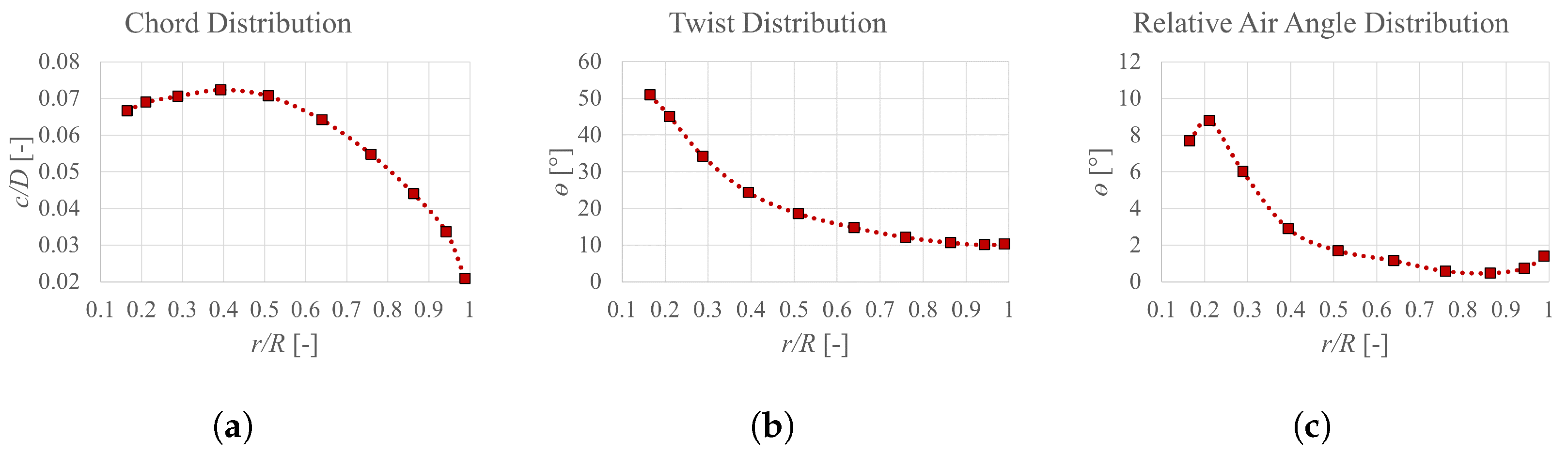
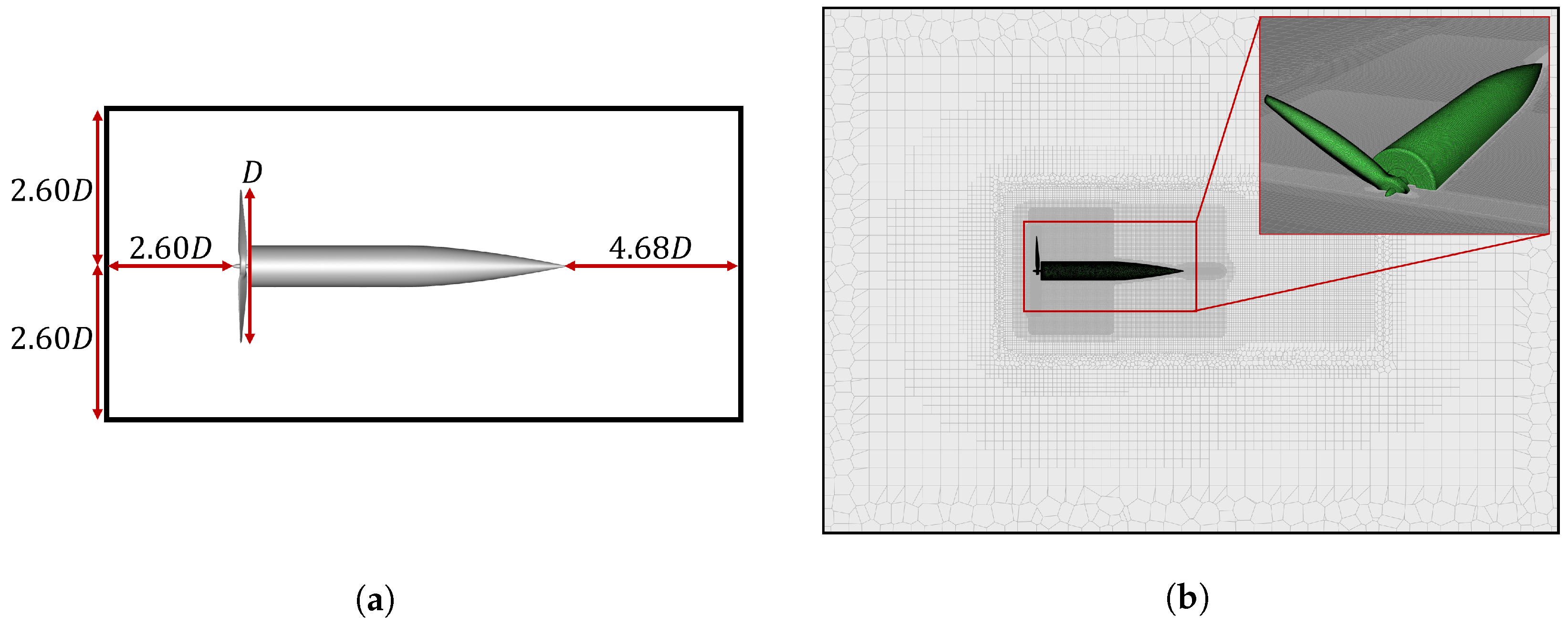
2.2. Demonstration Case Setup

In this paper, a low-Reynolds-number propeller was used as a demonstration case. This propeller was a benchmark configuration that has been widely employed in previous numerical and experimental studies on propeller noise modeling and reduction [17,19,27,28]. As shown in Figure 1, the propeller configuration consisted of a counter-clockwise two-bladed propeller mounted at the front of a cylindrical nacelle. The same propeller dimensions and installation setup have been used in previous research [19,27]. The propeller presented a diameter of $D=9^{″}$ with a pitch-to-diameter ratio of $P/D=1$, and the two blades were characterized by the cross-sections of Clark-Y airfoil. Figure 2 shows the distributions of blade characteristics along the radium R. In addition, the cylindrical nacelle presented dimensions of $L=400$ mm in length and $d=65$ mm in diameter. The tail part of the nacelle is streamlined to prevent the effect of massive wake.

In the present simulations, the propeller was operated at sea level with a rotating speed of 6500 rev/min and a forward-flight speed of 12 m/s, corresponding to an advance ratio of $J=0.485$. Previous experiment measurements [27] showed that the same propeller configuration produced the largest mean thrust coefficient around this advance ratio. The Reynolds number of the propeller flow was $Re=4.8\times {10}^4$ and the Mach number was $M=0.231$. In this flow condition, the flow was characterized by turbulence and weak compressibility, as expected, and the relative air angle at various blade positions was determined to be ${0.465}^{\circ }$ to ${8.794}^{\circ }$ (as shown in Figure 2c). The following assumptions were made based on the characteristics of the Clark-Y airfoil and the small relative angles to the freestream: the time-averaged lift coefficients $\overline{C_L}$ of the propeller blade cross-sections were approximately proportional to the relative angle, and the time-averaged drag coefficients $\overline{C_D}$ were approximately constant. Despite these aerodynamic coefficients being obtainable from flow modeling, this approximation was used when performing Hanson’s method to reduce computational costs.

Numerical Setup in Flow Modeling

Figure 3 shows the numerical setup of the LES calculation. The propeller configuration was placed in a computation domain featuring a square cylinder, which presented a length of $9.21D$ in the streamwise direction and are a length of $5.20D$ in the spanwise and transverse directions. Three-dimensional Cartesian coordinates were used to define the domain space, with the x, y, and z-axis aligned with the streamwise, spanwise, and transverse directions, respectively. The origin of the coordinate system was positioned at the center of the nacelle, $0.90D$ downstream from the propeller. A far-field pressure boundary condition was applied to both the upstream and downstream boundaries to produce a freestream at 12 m/s. A non-slip wall boundary condition was applied to the surfaces of the propeller configuration, and a pressure outlet boundary condition was set for the remaining boundaries. To prevent numerical errors due to acoustic reflections, a general non-reflective boundary condition (NRBC) using Riemann’s method was applied at the outer boundaries.

The computational domain was meshed using poly-hex cells. Figure 3b presents the cell distribution in the computational domain, as well as close to the propeller. The mesh size over the propeller surfaces was set as $y^{+}=1$ and ${\Delta }_{x,z}^{+}=36-200$ in a dimensionless wall unit. And the meshes in the propeller wake were refined, which had a size of $0.007D$ in the wake $x/D\le 1$ and $0.014D$ for $x/D\le 2$. For time marching, the solution was advanced with a physical time step of $1\times {10}^{-5}$ s, corresponding to ${0.39}^{\circ }$ of the propeller rotating angle. The simulation reached time-stationary after 13 propeller revolutions. Then, the simulation was further run for 4 revolutions to collect data for analysis. Although the present cell count and the time step were relatively coarser than those of a wall-resolved LES, it was efficient for resolving energy-containing eddies, so that most of the turbulent kinetic energy was resolved and the computational cost was reduced.

3. Results

3.1. Propeller Aerodynamics

Figure 4 provides a perspective view of the flow field of the propeller configuration using the distribution of the instantaneous vorticity magnitude on the iso-surfaces of the normalized Q-criterion $Q=0.3$ and in the mid-plane $y=0$ m. The propeller flow was characterized by dominant flow structures of significant tip vortices, which were generated at the blade tips, and small-sale vortices, which were detached from the blade trailing edges. These two vortical structures moved downstream with the main flow, to form propeller wake, as well as being less structural. In addition, small-scale vortical structures were observed as being formed over the nacelle surfaces and interacting with the tip vortices further downstream.

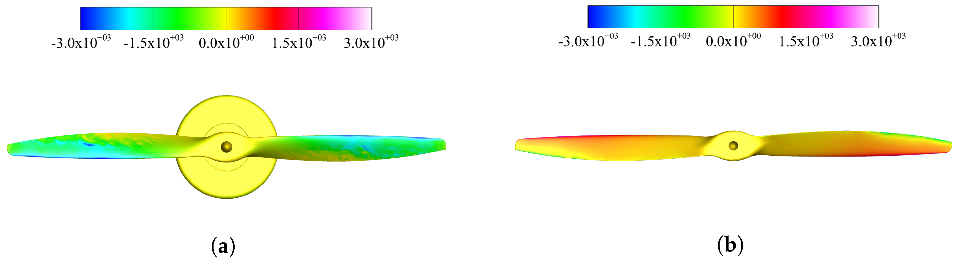
3.1.1. Aerodynamic Loading

The aerodynamic loading on the propeller surfaces was obtained through LES calculations and validated against experimental measurements [27]. The integral of the aerodynamic force in the streamwise direction was defined as the propeller thrust T, and the integral of the moment of the force about the x-axis was defined as the propeller torque Q.

Table 1. Time-averaged values of propeller thrust and torque.

	Present (LES)	Experiment *	Difference
$\overline{T}$ [N]	2.9205	2.8197	$+3.57\%$
$\overline{Q}$ [N·m]	0.0964	0.0976	$-1.23\%$

* Experimental results are cited from [27].

presents the results for time-averaged thrust, $\overline{T}$, and torque, $\overline{Q}$, and compares them with existing experimental measurements [27]. The averaged values were calculated using algebraic averaging, with a sampling frequency of $5\times {10}^4$ Hz and a sampling time covering two rotational cycles. The differences between the LES and experimental results were minimal (no more than $3.57\%$), indicating that the present LES effectively modeled the propeller’s aerodynamic loading. Therefore, the aerodynamic inputs for Hanson’s and Gutin’s models were verified.

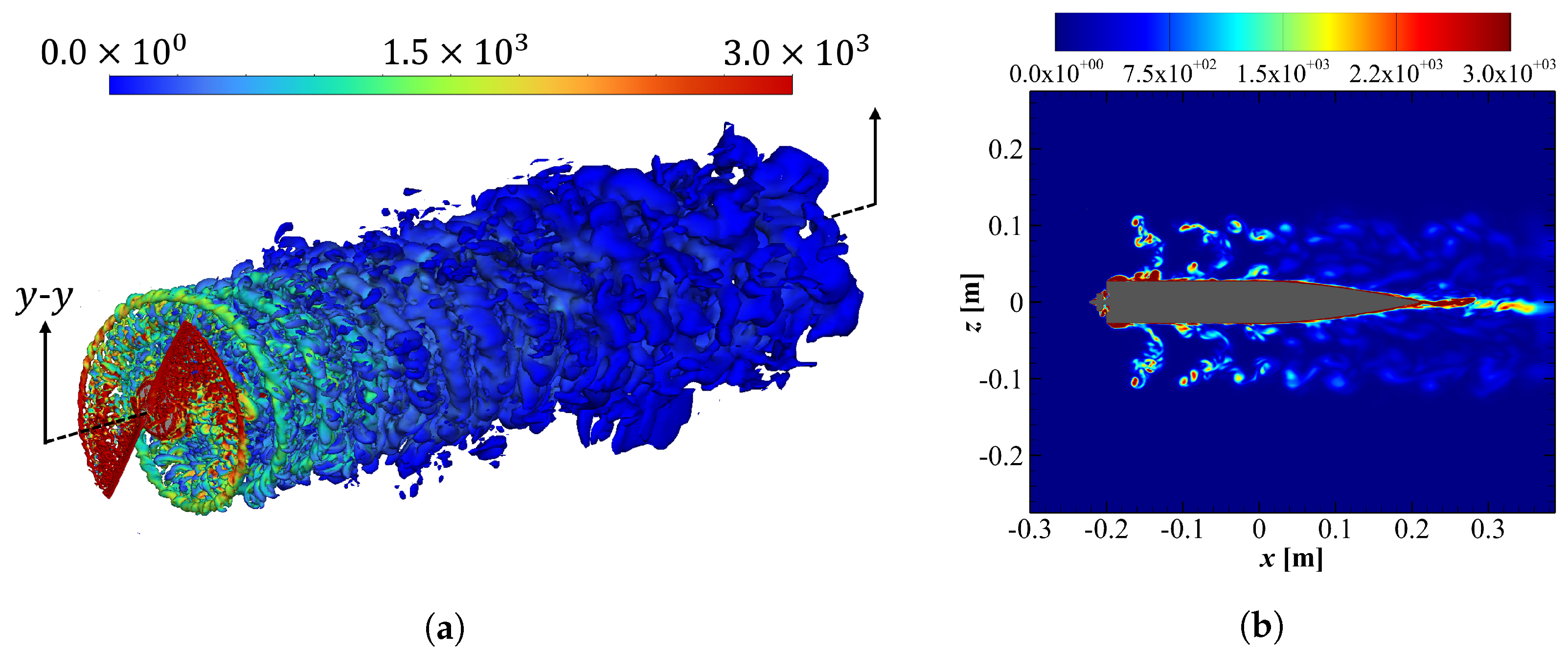
3.1.2. Flow Features

Figure 5 shows the instantaneous velocity distributions in the mid-plane $y=0$ m, where u, v, and w denote the velocity components in the streamwise, transverse, and spanwise directions, respectively. The u-field presented the highest velocity magnitudes among the three components. A significant jet flow was induced by the propeller motion, associated with the thrust generation. On the contrary, the w-field presented the lowest velocity magnitudes, indicating the flow had relatively weak radial velocity as compared with the axial and the rotational velocities. In addition, the v-field presented velocity magnitudes in the jet flow region with opposite signs about the rotating axis. Strong rotational velocity was observed in the tip vortices which surrounded the jet flow.

Figure 6 presents the distribution of instantaneous pressure, p, on the front and the rear sides of the blade surfaces. Lower and higher pressure magnitudes were, respectively, generated on the front (suction) and the rear (pressure) sides, which resulted in a positive propeller thrust. On the front sides of blades, the lowest pressure magnitudes occurred at the leading edges of the blades, spanning between the middle and the outboard sections, and additional lower pressure magnitudes were observed as pressure footprints in the middle of the blade surfaces. These patterns indicate that the flow over the front side separated at the blade leading edges due to an inverse pressure gradient, generated vortical structures, and reattached again on the blades [29,30]. Similar separating and reattaching flow have previously been observed in the flow of low-Reynolds-number propellers, and the mechanism was attributed to the separation and transition of laminar boundary layers over propeller blades [22]. This separation and the induced vortices brought significant fluctuations to the boundary layers on the propeller blades and, as a result, intensified the unsteadiness in the boundary layers and the generation of small-scale vortices at the blade trailing edges [30]. On the rear sides of the blades, the highest pressure magnitudes occurred at the leading edges between the middle and the outboard blade sections. In addition, relatively low pressure magnitudes were observed at the trailing edges, which probably resulted from the small-scale vortices on the front sides passing over the trailing edges.

3.2. Far-Field Noise

The far-field noise obtained from the three models was measured by a microphone array. As shown in Figure 7, the microphones were placed in an arch shape in a polar direction, ranging from $\theta =0^{\circ }$ to ${180}^{\circ }$. The same microphone setup was used in previous studies [17,19,27,28]. The radium of the arch was 1.75 m (equal to $7.66D$) from the propeller center, considered to be sufficiently far for recording acoustic signals at far-field. The angular interval between neighboring microphones was prescribed to be $\Delta \theta =5^{\circ }$, leading to 37 microphones in total.

3.2.1. Tonal Noise

The tonal component of propeller noise is associated with propeller rotational motion. Therefore, it is dominated by tones at the blade passing frequency ($\mathrm{BPF}=216.67$ Hz) and its positive integer multiple. The magnitude of tonal noise is described by sound pressure level (SPL), which is defined as follows:

$$\mathrm{SPL}=10\times {\log }_{10}(p_a^2/p_0^2)\left[\mathrm{dB}\right]$$

(7)

where $p_a$ denotes sound pressure and $p_0=2\times {10}^{-5}$ [pa] is the reference sound pressure. Figure 8 presents the spectra of the blade-passing tones measured in the directions of $\theta ={90}^{\circ }$ and ${120}^{\circ }$, and makes comparisons with the experimental measurements [27]. The selection of these two directions was based on the limitations of Gutin’s method. The first harmonic of the blade-passing tone appeared to be the dominant component of the tonal noise, while the higher harmonics of the BPF showed relatively lower SPL. All three methods managed to predict the first harmonic. The FWH method provided the best prediction of the first harmonic, whilst showing overestimation of the SPL of the higher harmonics. This overestimation probably resulted from the use of a shorter sampling time. In contrast, Hanson’s method performed the best in predicting the higher harmonics, even with a slight underestimation of the harmonics higher than the third. Gutin’s method also offered a good prediction for the first harmonic, despite having lower accuracy for the higher harmonics.

Figure 9 presents the SPL directivity of the first two blade-passing harmonics. The first harmonic presented a dipole shape, with the direcitvity at approximately $\theta ={120}^{\circ }$, while the second harmonic had less pattern features of directivity. The FWH method demonstrated a good capability for predicting the first harmonic. However, for the second harmonic, the FWH method provided reasonable accuracy only for $\theta <{120}^{\circ }$, with slight underestimation as $\theta$ exceeded ${120}^{\circ }$. In contrast, Hanson’s method showed a relatively good agreement with the experimental measurements, with minor overestimation around $\theta ={75}^{\circ }$ for the first harmonic and around $\theta ={60}^{\circ }$ for the second harmonic. On the other hand, Gutin’s method did not yield reliable directivity results. Only the first harmonic results were reasonable, as they fell within the method’s valid directional range (${90}^{\circ }\le \theta \le {120}^{\circ }$).

3.2.2. Broadband Noise

Only the results from the FWH method are presented to investigate broadband noise, as Hanson’s and Gution’s method do not consider broadband noise. Figure 10 presents the power spectral density (PSD) spectra of sound pressure at $\theta ={90}^{\circ }$ and ${60}^{\circ }$. The PSD spectra were calculated using the direct fast Fourier transform (FFT) with a sampling frequency of $5\times {10}^4$ Hz and a sampling time corresponding to four propeller revolutions. The FWH results were comparable with the experimental measurements at $f<2\times {10}^3$ Hz but showed increasing overestimation at $f>2\times {10}^3$ Hz. The overestimation at high frequency ranges may have resulted from unsolved energy in small eddies. Clear frequency peaks occurred at the blade passing frequency, and relatively significant broadband components were observed. This indicates that the broadband noise contributed considerable power to the propeller noise and may not be ignored in this case. Furthermore, the spectral magnitude of BPF was greater at $\theta ={90}^{\circ }$, while the magnitudes of the broadband components were relatively greater at $\theta ={60}^{\circ }$. This is aligned with the directivity plots in Figure 9 and suggests the broadband noise had greater intensity in the streamwise direction.

3.2.3. Overall Noise

The magnitude of overall propeller noise is described using overall sound pressure level (OASPL), which is calculated by the integration of sound power over a defined frequency range.

$$\mathrm{OASPL}=10\times {\log }_{10}({\int }_{f_1}^{f_2}{p}_a^2\left(f\right)\mathrm{d}f/p_0^2)\left[\mathrm{dB}\right]$$

(8)

where $f_1$ and $f_2$ define the frequency range of integration. The OASPL results from the FWH method were computed using the frequency range from 0.33 to 50 times BPF, which was the same as used for treating the experimental results [27]. For the results from Hanson’s and Gutin’s methods, the OASPL was computed by integrating the first 10 harmonics of the blade passing tone.

Figure 11 presents the OASPL directivity of the overall noise, showing that the three models achieved different overall noise features. The FWH result agreed most closely with the experimental results, showing the highest OASPL magnitudes at streamwise directions and no predominant directivity. On the contrary, the Hanson method result captured the OASPL magnitudes in the vertical direction ${60}^{\circ }<\theta <{120}^{\circ }$ but underestimated the magnitudes in the rest of the regions, especially for the streamwise direction. The OASPL directivity of the Hanson method result presented a dipole in the vertical direction, with similar patterns as for the tonal noise directivity in Figure 9. The difference of the Hanson method result was possibly due to the omission of broadband noise, which was significant in this case and particularly intensive in the streamwise directions. For the Gutin method results, the OASPL magnitudes at ${90}^{\circ }<\theta <{120}^{\circ }$ were relatively comparable to the experimental results.

4. Discussion

4.1. On the Mechanism of Noise Generation and Radiation

The propeller flow was characterized by significant tip vortices, weak separation over the blade suction sides, and unsteady boundary layers over the blade surfaces. Similar flow features were reported in previous studies on low-Reynolds-number propellers [22]. Tonal and broadband noise were observed in the far-field noise. The mechanism of the noise generation and radiation can be explained using existing propeller aeroacoustic theories and associated with the flow features [15,31].

The tonal noise was associated with the rotating motion of the propeller and consisted of thickness noise and loading noise. The thickness noise sources were generated by the displacement of the blade volumes and, hence, were monopole sources. For an isolated propeller parallel to the mainstream, the loading noise is approximately the steady loading noise. Steady loading noise sources are generated by the displacement of steady loadings on the blades and, therefore, are dipole sources. For subsonic flow, the tonal noise modes cannot propagate in the axial direction [15]. This coincides with the tonal noise in the present case being stronger in the transverse direction. On the other hand, the broadband noise was attributed to trailing edge noise. Trailing edge noise is generated when unsteady boundary layers pass blunt trailing edges and is a significant noise source with broadband frequencies at low Mach numbers [31]. Trailing edge noise is radiated vertical to the trailing edge, which coincides that the broadband noise in the present case being stronger in the streamwise direction, as the propeller blades had a small pitch [31].

4.2. On the Capacities of the Three Noise Modeling Methods

The capacities of the three noise models for predicting this kind of propeller noise are discussed regarding their application, accuracy, and computational costs:

-

Gutin’s method: Gutin’s method presented considerable accuracy in predicting the magnitudes of the first BPF harmonic in the vertical direction, with difference of 1.55–4.08 dB. The accuracy decreased as the harmonic order increased. This method can be used to roughly estimate the OASPL noise in the vertical direction for cases with similar aeroacoustic features as this work. Gutin’s method is computationally efficient, owing to the tabular calculation and simple inputs required [2]. It uses the propeller blade number, diameter, blade area, and flight speeds to describe the problem setup, and the steady and integral values of the propeller thrust and power as aerodynamics inputs [10]. Therefore, Gutin’s method would be ideal for aircraft conceptional design, where the blade characteristics are not identified, and performed together with low-fidelity flow modeling [2].

-

Hanson’s method: Hanson’s method shows good accuracy in predicting tonal noise, in terms of the magnitudes of the blade passing harmonics and the SPL directivity. This method can be used to estimate the OASPL noise in the vertical direction (with a difference of around 2.84 dB) for cases with similar aeroacoustic features to this work, but not in the streamwise direction, where broadband noise dominates. Hanson’s method requires more inputs for computation than Gutin’s method. Additional inputs include propeller blade profiles and relative air angles for the problem setup, as well as the distributions of drag and the lift coefficients as the aerodynamic inputs [14].

-

The FWH method: The FWH method presents good accuracy in predicting both tonal noise and broadband noise. The overestimation of sound pressure at high-frequency components and high-order BPF harmonics may be corrected using a finer mesh and longer sampling times. In general, this method is suitable for cases where the broadband noise is significant with respect to the overall propeller noise. On the other hand, the FWH method is much more computationally intensive, four- and three-orders, respectively, higher than Gutin’s and Hanson’s methods. It needs to be performed together with high-fidelity flow modeling. Spacial and temporal flow solutions are required as the aerodynamics inputs, the amount of which are proportional to the mesh number of the FWH integral surfaces and the sampling time step number [16].

A tabular summary of the capacities of the three noise models is shown in

Table 2. Capacity of three acoustic models for modeling propeller noise.

Acoustic Model	BPF Tone	Higher Harmonics	Broadband Noise	Noise Directivity	Computational Time Factor
Gutin’s	Good	Poor	n/a	n/a	1
Hanson’s	Good	Good	n/a	Poor	$O\left({10}^1\right)$
FWH	Good	Fair	Good	Good	$O\left({10}^4\right)$

.

5. Conclusions

In this paper, a comparison study of three multi-fidelity noise models was conducted for predicting the aeroacoustics of a benchmark low-Reynolds-number propeller $Re=4.8\times {10}^4$. The Ffowcs-Williams and Hawkings (FWH), Hanson, and Gutin methods were assessed as, respectively, the high-, medium-, and low-fidelity noise models. A coarse-grid LES calculation was performed to investigate the propeller aerodynamics and to obtain the aerodynamic inputs for these three noise models.

The flow and noise features of the propeller were observed using coarse-grid LES and the FWH method. Then, the mechanisms of the aerodynamic noise generation and radiation were clarified using existing aeroacoustic theories. The propeller flow was characterized by significant tip vortices, weak separation over the blade suction sides, and unsteady boundary layers over the blade trailing edges. The far-field noise was dominated by the tonal components in the vertical direction and by the broadband components in the streamwise direction. The tonal noise was generated by thickness and loading noise sources, and broadband noise was generated mainly by the unsteady boundary layers as trailing-edge noise.

The FWH method showed the best accuracy in predicting the magnitudes and directivity of both the BPF noise and broadband noise. However, the calculation using the FWH method required more computational time, approximately three-orders higher, than the other two. On the contrary, Hanson’s method presented great efficiency in predicting the magnitudes and the directivity of the tonal noise. Gutin’s method was mainly capable of predicting BPF noise in the vertical direction. However, Gutin’s method had outstanding advantages in using the least computational time and for the input information of propeller geometry and aerodynamics. Although Hanson’s and Gutin’s methods do not account for broadband noise, they may still be applicable for estimating the OASPL of noise propagating in the transverse direction, as broadband noise mainly propagates in the streamwise direction.

Indeed, the characteristics of propeller noise differ in different physical situations. The test case in this paper had one of the aeroacoustic features that contributes to variations in the noise generation from low-Reynolds-number propellers, i.e., broadband noise generated by unsteady boundary layers over the propeller blades. Owning to a thorough understanding of the physical situation, the conclusions achieved in this paper can be applicable to a broad range of cases with similar flow and noise characteristics.

In future work, cases at higher Reynolds and Mach numbers, such as open rotor configurations, will be investigated. Furthermore, models for predicting broadband noise will be assessed to complement Hanson’s method, and lower-fidelity flow models will be included in this multi-fidelity framework.

References

1. Baledón, M.S.; Kosoy, N. “Problematizing” carbon emissions from international aviation and the role of alternative jet fuels in meeting ICAO’s mid-century aspirational goals. J. Air Transp. Manag. 2018, 71, 130–137. [Google Scholar] [CrossRef] [PubMed]
2. Guynn, M.D.; Berton, J.J.; Haller, W.J.; Hendricks, E.S.; Tong, M.T. Performance and Environmental Assessment of an Advanced Aircraft with Open Rotor Propulsion; Technical Report; NASA: Washington, DC, USA, 2012.
3. Silva, C.; Johnson, W.R.; Solis, E.; Patterson, M.D.; Antcliff, K.R. VTOL urban air mobility concept vehicles for technology development. In Proceedings of the 2018 Aviation Technology, Integration, and Operations Conference, Atlanta, GA, USA, 25–29 June 2018; p. 3847. [Google Scholar]
4. Kurtz, D.; Marte, J. A Review of Aerodynamic Noise from Propellers, Rotors, and Lift Fans; NASA: Washington, DC, USA, 1970.
5. Schlegel, R.; King, R.; Mull, H. Helicopter Rotor Noise Generation and Propagation; Citeseer: Alexandria, VA, USA, 1966. [Google Scholar]
6. Lowson, M.; Ollerhead, J. A theoretical study of helicopter rotor noise. J. Sound Vib. 1969, 9, 197–222. [Google Scholar] [CrossRef]
7. Wright, S. The acoustic spectrum of axial flow machines. J. Sound Vib. 1976, 45, 165–223. [Google Scholar] [CrossRef]
8. Farassat, F. Advanced Theoretical Treatment of Propeller Noise; Lecture Series; von Karman Institute for Fluid Dynamics: Sint-Genesius-Rode, Belgium, 1982; pp. 81–82. [Google Scholar]
9. Gutin, L. On the Sound Field of a Rotating Propeller; Physikalische Zeitschrit der Sowjetinion: Physical Magazine of the Soviet Union Volume 9 Number 1; NASA: Washington, DC, USA, 1948; Volume 9.
10. Aircraft Noise Committee. Estimation of the Maximum Discrete Frequency Noise from Isolated Rotors and Propellers; Technical Report; Tech Rep Aerounautical Series 76020; ESDU: London, UK, 2011.
11. Hanson, D.B.; Fink, M.R. The importance of quadrupole sources in prediction of transonic tip speed propeller noise. J. Sound Vib. 1979, 62, 19–38. [Google Scholar] [CrossRef]
12. Hanson, D.B. Helicoidal surface theory for harmonic noise of propellers in the far field. AIAA J. 1980, 18, 1213–1220. [Google Scholar] [CrossRef]
13. Hanson, D.B.; Parzych, D.J. Theory for Noise of Propellers in Angular Inflow with Parametric Studies and Experimental Verification; Technical Report; NASA: Washington, DC, USA, 1993.
14. Aircraft Noise Committee. Prediction of Near-Field and Far-Field Harmonic Noise from Subsonic Propellers with Non-Axial Inflow; Technical Report; Tech Rep Aerounautical Series 11005; ESDU: London, UK, 2018.
15. Peake, N.; Parry, A.B. Modern challenges facing turbomachinery aeroacoustics. Annu. Rev. Fluid Mech. 2012, 44, 227–248. [Google Scholar] [CrossRef]
16. Lele, S.K.; Nichols, J.W. A second golden age of aeroacoustics? Philos. Trans. R. Soc. A Math. Phys. Eng. Sci. 2014, 372, 20130321. [Google Scholar] [CrossRef] [PubMed]
17. Huang, G.; Sharma, S.; Ambrose, S.; Jefferson-Loveday, R. Numerical study on the aeroacoustics of a propeller-wing integration at various advance ratios. In Proceedings of the Turbo Expo: Power for Land, Sea, and Air; American Society of Mechanical Engineers: Houston, TX, USA, 2023; Volume 86939, p. V001T01A024. [Google Scholar]
18. Huang, D.; Yang, Z.; Leung, R.C.K. Implementation of direct acoustic simulation using ANSYS Fluent. In Proceedings of the INTER-NOISE and NOISE-CON Congress and Conference Proceedings, Washington, DC, USA, 1–5 August 2021; Institute of Noise Control Engineering: Wakefield, MA, USA, 2021; Volume 263, pp. 1243–1252. [Google Scholar]
19. Sharma, S.; Huang, G.; Ambrose, S.; Jefferson-Loveday, R. Numerical study on the aeroacoustics and interaction of two distributed-propulsion propellers in co-and counter-rotations. Proc. Mtgs. Acoust. 2022, 50, 030002. [Google Scholar]
20. Kotwicz Herniczek, M.T.; Feszty, D.; Meslioui, S.A.; Park, J.; Nitzsche, F. Evaluation of acoustic frequency methods for the prediction of propeller noise. AIAA J. 2019, 57, 2465–2478. [Google Scholar] [CrossRef]
21. Bergmann, O.; Möhren, F.; Braun, C.; Janser, F. Comparison of Various Aeroacoustic Propeller Noise Prediction Methodologies in Static Operations. In Proceedings of the AIAA SciTech 2022 Forum, San Diego, CA, USA, 3–7 January 2022; p. 2529. [Google Scholar]
22. Candeloro, P.; Ragni, D.; Pagliaroli, T. Small-scale rotor aeroacoustics for drone propulsion: A review of noise sources and control strategies. Fluids 2022, 7, 279. [Google Scholar] [CrossRef]
23. Huang, G.; Sharma, A.; Chen, X.; Riaz, A.; Jefferson-Loveday, R. Framework for Multi-Fidelity Assessment of Open Rotor Propeller Aeroacoustics. In Proceedings of the 30th AIAA/CEAS Aeroacoustics Conference (2024), Roma, Italy, 4–7 June 2024; p. 3098. [Google Scholar]
24. Lighthill, M.J. On sound generated aerodynamically I. General theory. Proc. R. Soc. Lond. Ser. A Math. Phys. Sci. 1952, 211, 564–587. [Google Scholar]
25. Huang, G.; Sharma, S.; Ambrose, S.; Jefferson-Loveday, R. Numerical Prediction of Aerodynamic Noise for a Propeller-wing Configuration and an Investigation of Pitch Effect. In Proceedings of the INTER-NOISE and NOISE-CON Congress and Conference Proceedings, Institute of Noise Control Engineering, Tokyo, Japan, 20–23 August 2023; Volume 268, pp. 7475–7486. [Google Scholar]
26. Ffowcs Williams, J.E.; Hawkings, D.L. Sound generation by turbulence and surfaces in arbitrary motion. Philos. Trans. R. Soc. Lond. Ser. A Math. Phys. Sci. 1969, 264, 321–342. [Google Scholar]
27. Jamaluddin, N.S.; Celik, A.; Baskaran, K.; Rezgui, D.; Azarpeyvand, M. Experimental characterisation of small-scaled propeller-wing interaction noise. In Proceedings of the 28th AIAA/CEAS Aeroacoustics 2022 Conference, Southampton, UK, 14–17 June 2022; p. 2973. [Google Scholar]
28. Turhan, B.; Kamliya Jawahar, H.; Bowen, L.; Rezgui, D.; Azarpeyvand, M. Aeroacoustic characteristics of distributed electric propulsion system in forward flight. In Proceedings of the AIAA AVIATION 2023 Forum, San Diego, CA, USA, 12–16 June 2023; p. 4490. [Google Scholar]
29. Lee, D.; Kawai, S.; Nonomura, T.; Anyoji, M.; Aono, H.; Oyama, A.; Asai, K.; Fujii, K. Mechanisms of surface pressure distribution within a laminar separation bubble at different Reynolds numbers. Phys. Fluids 2015, 27, 023602. [Google Scholar] [CrossRef]
30. Thompson, M.C. Effective transition of steady flow over a square leading-edge plate. J. Fluid Mech. 2012, 698, 335–357. [Google Scholar] [CrossRef]
31. Williams, J.F.; Hall, L. Aerodynamic sound generation by turbulent flow in the vicinity of a scattering half plane. J. Fluid Mech. 1970, 40, 657–670. [Google Scholar] [CrossRef]
Figure 1. Illustration of the benchmark propeller configuration operated at low Reynolds numbers.
Aerospace 12 00154 g001
Figure 2. Distributions of the blade characteristics along the radium: (a) chord c / D , (b) twist β , and (c) relative air angle α .
Aerospace 12 00154 g002
Figure 3. Demonstration of the numerical setup: (a) schematics of the square-cylinder computational domain (dimensions not to scale) and (b) the distribution of surface and volume meshes.
Aerospace 12 00154 g003
Figure 4. Distributions of vorticity magnitudes [m/s2] (a) on the iso-surfaces of the normalized Q-criterion Q = 0.3 and (b) in the mid-plane y = 0 m.
Aerospace 12 00154 g004
Figure 5. Distributions of instantaneous velocity components [m/s], (a) u, (b) v, and (c) w, in the mid-plane y = 0 m.
Aerospace 12 00154 g005
Figure 6. Distribution of instantaneous pressure p [pa] on the propeller surfaces: (a) the front side and (b) the rear side.
Aerospace 12 00154 g006
Figure 7. Schematics of the far-field microphone locations related to the propeller configuration, where red circles represent the microphones (dimensions not to scale).
Aerospace 12 00154 g007
Figure 8. Spectra of tonal noise at (a) θ = 90 and (b) θ = 120 . Experimental results cited from [27].
Aerospace 12 00154 g008
Figure 9. Directivity of blade passing tones in [dB]: (a) the first harmonic and (b) the second harmonic. Experimental results cited from [27].
Aerospace 12 00154 g009
Figure 10. Spectra of sound pressure PSD [dB/Hz] measured at (a) θ = 60 and (b) θ = 90 . Experimental results cited from [27].
Aerospace 12 00154 g010
Figure 11. Directivity of overall noise in OASPL [dB]. Experimental results cited from [27].
Aerospace 12 00154 g011