Nanosatellite Autonomous Navigation via Extreme Learning Machine Using Magnetometer Measurements

Abstract

This work presents an algorithm to perform autonomous navigation in spacecraft using onboard magnetometer data during GPS outages. An Extended Kalman Filter (EKF) exploiting magnetic field measurements is combined with a Single-Hidden-Layer Feedforward Neural Network (SLFN) trained via the Extreme Learning Machine to improve the accuracy of the state estimate. The SLFN is trained using GPS data when available and predicts the state correction to be applied to the EKF estimates. The CHAOS-7 magnetic field model is used to generate the magnetometer measurements, while a 13th-order IGRF model is exploited by the EKF. Tests on simulated data showed that the algorithm improved the state estimate provided by the EKF by a factor of 2.4 for a total of 51 days when trained on 5 days of GPS data.

1. Introduction

Spacecraft tracking is usually performed through ground-based tracking systems such as radar or optical station networks. The complexity introduced by these devices can be tackled by implementing autonomous navigation modules onboard spacecraft. This step is particularly crucial for small satellite missions, which generally have limited computational and power consumption resources available. An onboard GPS module is a common solution; however, it relies on the quality and the availability of the GPS signal for the accuracy of position and velocity estimates, thus making the satellite not completely autonomous. Furthermore, commercial GPS modules are subject to several limitations, such as military and/or government restrictions, intentional performance degradation, signal occlusion by the Earth during the initial acquisition phase, unwanted Doppler shifts, or component degradation [1].

For this reason, the use of data coming from sensors already available onboard, like magnetometers and/or Sun sensors, is attracting a lot of research effort [1,2,3,4]. Magnetometers, in particular, are low-cost sensors which can be exploited by Kalman Filters (KFs) [5,6,7] to perform autonomous orbit determination. This approach yields errors with accuracies ranging from hundreds of kilometers to sub-kilometers from the spacecraft’s position. The goodness of these estimates mainly depends on the accuracy of the magnetic field model used [8,9,10]. These results indicate that Kalman Filtering is a solid baseline for autonomous orbit determination, but the state estimation provided is still not reliable enough to be used in the absence of GPS signals. Following the recent exploit of Machine Learning (ML), many studies have been carried out to integrate Kalman Filtering with Artifical Intelligence (AI) frameworks, in particular by using Neural Networks (NNs). The reference [11] presents a detailed overview of ML-KF applications, paying particular attention to the different roles played by ML. Such roles include the following:

• Tuning and predicting KF parameters, such as error covariances;
• Predicting and compensating KF errors;
• Predicting and updating the state vector and/or measurements;
• Predicting pseudo-measurements to be fed to the KF.

In general, an hybrid approach shows better results than the application of standalone ML frameworks or Kalman Filtering. When dealing with non-linear dynamics or non-Gaussian noises, ML models provide a better outcome than Kalman Filtering which, in turn, offers better interpretability with respect to end-to-end ML approaches. For most architectures, in fact, the intermediate relations between the features are unknown and the ML module acts as a “black box” between the input and the output of the process. 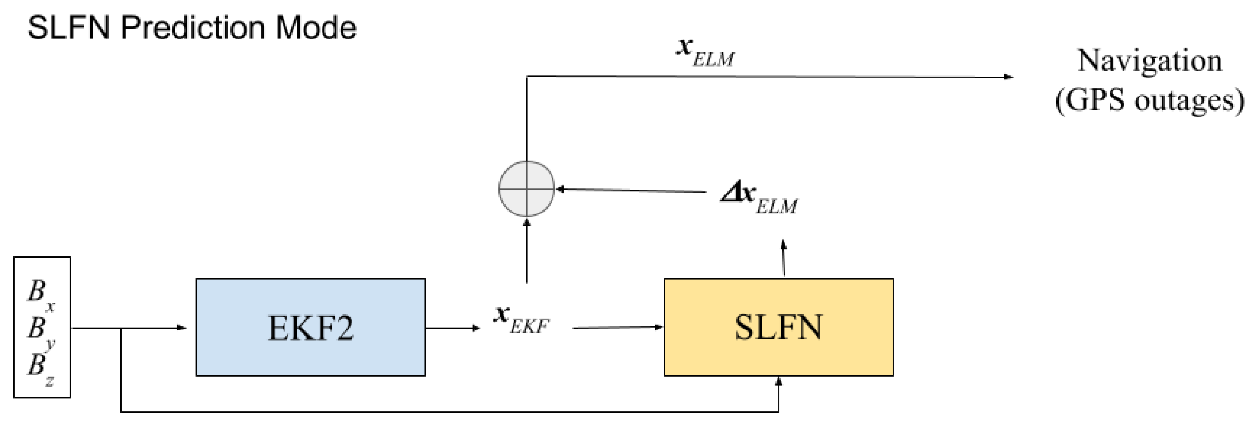In this work, the solidity and reliability of the Extended Kalman Filter (EKF) [12,13] is combined with a Neural Network trained via the Extreme Learning Machine [14,15] to further increase the accuracy of the state estimate. In particular, the algorithm collects GPS data as long as the GPS signal is available, while a magnetometer-based EKF provides a second, less accurate, state estimate. The error of the EKF estimate with respect to the GPS one is computed. When the GPS is no longer available, the Neural Network is trained using the EKF estimates as input values and the errors, with respect to the GPS, as target values.

This work also represents a feasibility study of improved autonomous magnetometer-based navigation during spacecraft’s safe mode when the GPS signal is unavailable due to safety reasons, system anomalies, a lack of communication, or hardware/software failures. In many situations, safe-mode navigation is performed via coarse orbit propagation from some initial conditions provided to the spacecraft by the ground station. This operation can be particularly demanding, especially when dealing with constellations of small satellites. Furthermore, communication with the ground station might be impossible under the given circumstances. On the contrary, sensor-based approaches such as the one described in this work do not require ground intervention. In particular, this approach represents an improvement over traditional EKF-based navigation using magnetometer data.

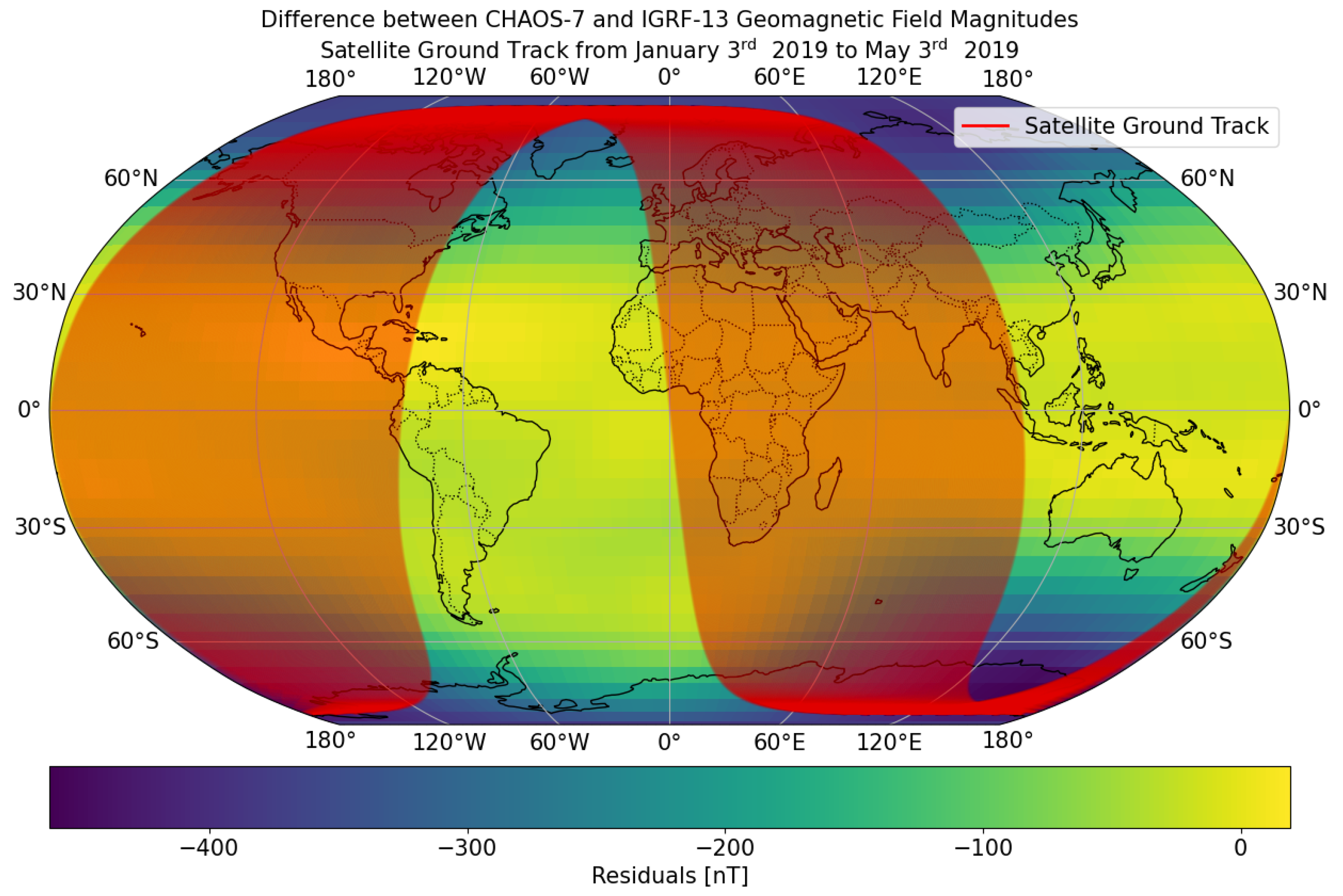
To meet onboard requirements such as limited power consumption and computational effort, the EKF employs an onboard IGRF magnetic field model to derive the state estimates, and it is aided by a Neural Network to overcome the model discrepancies with respect to the CHAOS-7 magnetic field. The overall process represents an accurate and lighter alternative to the direct implementation of the CHAOS-7 model in the EKF and a backup solution for the navigation of small satellites during GPS outages.

The algorithm was trained and tested on a simulated Sun-synchronous orbit considering J2, J3, third-body, and atmospheric-drag perturbations. The geomagnetic model used to provide the measurements was the CHAOS-7 magnetic field model [16], while the filter implemented a spherical harmonics expansion using the 13th-Generation International Geomagnetic Reference Field (IGRF) coefficients up to the 13th order [17]. This manuscript is organized as follows. Section 2 describes the main frameworks used in this work; Section 3 explains the parameter optimization process; Section 4 describes the dataset generation; and Section 5 presents the obtained results. Conclusions and future works on this topic are presented in Section 7 at the end of the manuscript.

2. Methodology

This section describes the two algorithms used in this work.

2.1. Extended Kalman Filter

The Extended Kalman Filter (EKF) [12,13] is a model-based, non-linear algorithm developed in the early 1960s [5]. The quality of its performance is strictly linked to the knowledge of the underlying dynamics and to the goodness of model assumptions. Here, the state vector ${\mathit{x}}_k$ in the k-th time step is represented by the position and the velocity of the spacecraft in an Earth-Centered Inertial (ECI) reference frame,

$${\mathit{x}}_k=[x,y,z,v_x,v_y,v_z],$$

(1)

while the observation vector ${\mathit{o}}_k$ is either given by the components of the geomagnetic field $B_x,B_y,B_z$,

$${\mathit{o}}_k^B=[B_x,B_y,B_z],$$

(2)

or by the GPS signal received by the spacecraft $GP{S}_x,GP{S}_y,GP{S}_z$,

$${\mathit{o}}_k^{GPS}=[GP{S}_x,GP{S}_y,GP{S}_z].$$

(3)

On the other hand, the observation vector is taken as a non-linear function, z, of the state plus a zero-mean random process, $\mathit{v}$:

$$\mathit{o}=z\left(\mathit{x}\right)+\mathit{v}$$

(4)

The time evolution of the state, instead, is a non-linear function, f, of the state plus another zero-mean random process, $\mathit{u}$:

$$\dot{\mathit{x}}=f\left(\mathit{x}\right)+\mathit{u}.$$

(5)

The new state estimate ${\widehat{\mathit{x}}}_k$ is given by the following equation according to the EKF theory:

$${\widehat{\mathit{x}}}_k={\overline{\mathit{x}}}_k+{\mathbf{K}}_k[{\mathit{o}}_k-z\left({\overline{\mathit{x}}}_k\right)],$$

(6)

where ${\overline{\mathit{x}}}_k$ is the state prediction, $\mathbf{K}$ indicates the Kalman gain matrix [18], and $[{\mathit{o}}_k-z\left({\overline{\mathit{x}}}_k\right)]$ is the residual: the difference between the actual measurement and the non-linear measurement prediction.

In the case of discrete measurements, Equation (4) can be rewritten as

$${\mathit{o}}_k=z\left({\mathit{x}}_k\right)+{\mathit{v}}_k.$$

(7)

To compute the Kalman gain matrix $\mathbf{K}$, a first-order approximation is used for the system dynamics matrix $\mathbf{F}$ and the measurement matrix $\mathbf{Z}$ since Equations (4) and (5) are non-linear. The relations between these matrices and the previous equations are

$${\mathbf{F}}_k={\displaystyle \frac{\partial f\left(\mathit{x}\right)}{\partial \mathit{x}}}{|}_{\mathit{x}={\widehat{\mathit{x}}}_k}$$

(8)

and

$${\mathbf{Z}}_k={\displaystyle \frac{\partial z\left(\mathit{x}\right)}{\partial \mathit{x}}}{|}_{\mathit{x}={\widehat{\mathit{x}}}_k}$$

(9)

The Kalman gain matrix can be computed from the Riccati equations, a set of recursive matrix equations given by [18]:

$$\begin{array}{c}{\mathbf{M}}_k={\mathsf{\Phi }}_{k-1}{\mathbf{P}}_{k-1}{\mathsf{\Phi }}_{k-1}^T+{\mathbf{Q}}_k\end{array}$$

(10)

$$\begin{array}{c}{\mathbf{K}}_k={\mathbf{M}}_k{\mathbf{Z}}_{k-1}^T{({\mathbf{Z}}_{k-1}{\mathbf{M}}_k{\mathbf{Z}}_{k-1}^T+{\mathit{R}}_k)}^{-1}\end{array}$$

(11)

$$\begin{array}{c}{\mathbf{P}}_k=(\mathbf{I}-{\mathbf{K}}_k{\mathbf{Z}}_{k-1}){\mathbf{M}}_k,\end{array}$$

(12)

where ${\mathsf{\Phi }}_{k-1}$ is the fundamental matrix and can be approximated by the first two terms of the Taylor-series expansion of $e^{{\mathbf{F}}_{k-1}{T}_s}$: ${\mathsf{\Phi }}_{\mathit{k}}\mathbf{\simeq }\mathit{I}+{\mathbf{F}}_{\mathit{k}\mathbf{-}\mathbf{1}}{\mathit{T}}_{\mathit{s}}$, with $T_s$ being the sampling time interval. The discrete process-noise matrix ${\mathbf{Q}}_k$ can be computed as

$${\mathbf{Q}}_{\mathit{k}}={\int }_0^{{\mathit{T}}_{\mathit{s}}}{\mathsf{\Phi }}_{\mathbf{k}\mathbf{-}\mathbf{1}}\left(\mathit{\tau }\right)\mathbf{Q}{\mathsf{\Phi }}_{\mathit{k}\mathbf{-}\mathbf{1}}^{\mathit{T}}\left(\mathit{\tau }\right)\mathit{d}\mathit{\tau },$$

(13)

where ${\mathsf{\Phi }}_{\mathit{k}\mathbf{-}\mathbf{1}}\left(\mathit{\tau }\right)=\mathbf{\simeq }\mathit{I}+{\mathbf{F}}_{\mathit{k}\mathbf{-}\mathbf{1}}\mathit{\tau }$.

Finally, the state prediction is given by

$${\overline{\mathit{x}}}_{\mathit{k}}={\mathsf{\Phi }}_{\mathit{k}\mathbf{-}\mathbf{1}}{\widehat{\mathit{x}}}_{\mathit{k}\mathbf{-}\mathbf{1}}\mathbf{.}$$

(14)

However, in the EKF, the state can be directly propagated forward by integrating the actual nonlinear differential equations in each sampling interval.

In this work, $f\left(\mathit{x}\right)$ is the state-dynamics function, including the $J_2$ perturbation, and $z\left(\mathit{x}\right)$ is the implemented pyIGRF [17] module to evaluate the magnetic field as a function of the position and time for the magnetometer-based EKFs, from which the matrix ${\mathbf{Z}}_B$ is computed numerically. On the other hand, the matrix $\mathbf{F}$ is obtained by deriving $f\left(\mathit{x}\right)$ analytically.

For the GPS-based EKF, the measurement function is

$${\mathbf{Z}}_{GPS}=\left[\begin{array}{cccccc}1& 0& 0& 0& 0& 0\\ 0& 1& 0& 0& 0& 0\\ 0& 0& 1& 0& 0& 0\end{array}\right],$$

(15)

which only maps the position into itself; therefore, the GPS-based EKF is a filter for the GPS noise.

2.2. Extreme Learning Machine

The Extreme Learning Machine (ELM) is a learning algorithm developed for Single-Hidden-Layer Feedforward Neural Networks (SLFNs) [14,15], known for its fast and lightweight nature. The main advantage of this learning algorithm is that if the activation function is infinitely differentiable in any interval, the input weights and biases can be sampled from any random distribution and kept fixed through the training procedure, still ensuring the convergence, as shown in [14]. In this way, the only parameters to be tuned are the output weights; therefore, the training process does not need an iterative tuning of the input weights and biases. The ideal number of hidden neurons, however, can be only determined empirically, as well as the amplitude of the distributions that the input weights and biases are sampled from. The absence of an iterative process drastically reduces the computational burden of the training phase, making the ELM an ideal solution when dealing with strict requirements in terms of hardware, as happens in the case of onboard applications. The architecture of an SLFN employing the ELM algorithm is shown in Figure 1.

Given an ELM-trained SLFN composed of M input neurons, L hidden neurons, J output neurons, an activation function, $g(·)$, and N training samples ($\mathbf{T}$, ${\mathbf{Y}}_{true}$), with $\mathbf{T}\in {\mathbb{R}}^{N\times M}$ and ${\mathbf{Y}}_{true}\in {\mathbb{R}}^{N\times J}$, the vector of the weights connecting the input neurons to the l-th hidden neuron can written as ${\mathit{w}}_l=[w_{1l},w_{2l},\dots ,w_{Ml}]$, and the weight connecting the l-th hidden neuron to the j-th output neuron is the quantity ${\beta }_{lj}$. Finally, let $b_l$ be the bias of the l-th hidden neuron. With these definitions, the j-th output with respect to the m-th input vector is expressed as

$$y_{mj}=\sum _{l=1}^L{\beta }_{lj}g({\mathbf{w}}_l·{\mathbf{t}}_m+b_l),$$

(16)

and, therefore, in matrix form, as

$$\mathit{y}=\mathbf{H}\mathit{\beta }$$

(17)

where $\mathbf{H}$ is the $N\times L$ matrix of the activation functions.

Let N be the number of training samples with target matrix ${\mathbf{Y}}_{true}$; the training process aims at finding the output weight matrix $\mathit{\beta }$ which minimizes the quantity $\left|\right|\mathbf{H}\mathit{\beta }-{\mathbf{Y}}_{true}\left|\right|$. Such an optimal matrix is given by the following smallest-norm least-square solution:

$$\widehat{\mathit{\beta }}={\mathbf{H}}^{†}{\mathbf{Y}}_{true},$$

(18)

where ${\mathbf{H}}^{†}$ is the Moore–Penrose generalized inverse matrix of $\mathbf{H}$.

3. Parameter Optimization

3.1. GPS-Based EKF Configuration

When available, the GPS data received by the satellite were processed by the first EKF, and a state vector, ${\mathit{x}}_{GPS}$, was returned. The EKF was run using the configuration shown in

Table 1. GPS-based Extended Kalman Filter configuration.

Parameter	Value
Measurement noise, ${\sigma }_{GPS}$	$0.033$ km
Initial position error, $\Delta x$	5 km $=3{\sigma }_x$
Initial velocity error, $\Delta v$	$0.5$ km/s $=3{\sigma }_v$
Process noise, $u_v$, $u_a$	0 km/s, ${10}^{-5}$ km/s2
Measurements noise matrix, ${\mathbf{R}}_{GPS}$	diag$\{{\sigma }_{GPS}^2,{\sigma }_{GPS}^2,{\sigma }_{GPS}^2\}$
Covariance matrix, $\mathbf{P}$	diag$\{{\sigma }_x^2,{\sigma }_x^2,{\sigma }_x^2,{\sigma }_v^2,{\sigma }_v^2,{\sigma }_v^2\}$
Process noise matrix, $\mathbf{Q}$	diag$\{w_v^2,w_v^2,w_v^2,w_a^2,w_a^2,w_a^2\}$
Measurement sampling time, $T_s^{GPS}$	1 s

.

The received GPS data ${\mathit{o}}_k^{GPS}=[GP{S}_x,GP{S}_y,GP{S}_z]$ were simulated by adding a zero-mean Gaussian noise, ${\mathit{GPS}}_{noise}$, with the standard deviation ${\sigma }_{GPS}$ to the real Cartesian position in the ECI of the spacecraft ${\mathit{r}}_{true}=[x_{true},y_{true},z_{true}]$ given by the propagated true orbit:

$${\mathit{o}}_k^{GPS}={\mathit{r}}_{true}+{\mathit{GPS}}_{noise}$$

(19)

3.2. Magnetometer-Based EKF Configuration

The magnetometer-based EKF was run using the configuration shown in

Table 2. Magnetometer-based Extended Kalman Filter configuration.

Parameter	Value
Measurement noise, ${\sigma }_B$	20 nT
Initial position error, $\Delta x$	5 km $=3{\sigma }_x$
Initial velocity error, $\Delta v$	$0.5$ km/s $=3{\sigma }_v$
Process noise, $u_v$, $u_a$	0 km/s, ${10}^{-5}$ km/s2
Model mismatch parameter, $\alpha$	1000 nT
Weight matrix, ${\mathbf{R}}_B$	diag$\{{\alpha }^2,{\alpha }^2,{\alpha }^2\}$
Covariance matrix, $\mathbf{P}$	diag$\{{\sigma }_x^2,{\sigma }_x^2,{\sigma }_x^2,{\sigma }_v^2,{\sigma }_v^2,{\sigma }_v^2\}$
Process noise matrix, $\mathbf{Q}$	diag$\{w_v^2,w_v^2,w_v^2,w_a^2,w_a^2,w_a^2\}$
Measurement sampling time, $T_s^B$	10 s

, where the best value for the measurement noise matrix ${\mathbf{R}}_B$ was determined in the following way.

In this work, the magnetometer measurements were simulated using the CHAOS-7 model described in Section 4.3.2 while the EKF computed the $\mathbf{Z}$ matrix using the IGRF magnetic field model (Section 4.3.1). The difference between the filter’s and measurements’ geomagnetic model was taken into account in the matrix ${\mathbf{R}}_B$ that was used as a weight matrix. Since complete knowledge of the noise process would require a perfect match between the two models, ${\mathbf{R}}_B$ was tuned by performing different runs with the EKF in order to find the best value to minimize the EKF errors. Figure 2 shows the results of different runs with different values in the model mismatch parameter $\alpha$ such as that ${\mathbf{R}}_B={\alpha }^2·{\mathbf{I}}_{3\times 3}$ in terms of the state mean and maximum Root Sum Squared Error (RSSE).

Similarly to the generation of the received GPS data, the magnetometer measurement vector ${\mathit{o}}_k^B=[B_x,B_y,B_z]$ was simulated by adding a zero-mean Gaussian noise, ${\mathit{B}}_{noise}$, with the standard deviation ${\sigma }_B=20$ nT to the magnetic field computed in the actual position of the spacecraft:

$${\mathit{o}}_k^B=\mathit{B}\left({\mathit{x}}_{true}\right)+{\mathit{B}}_{noise}.$$

(20)

The value of ${\sigma }_B$ was chosen according to the typical accuracy of onboard magnetometers [10,19,20,21].

3.3. Neural Network Configuration

This work used an SLFN trained via the ELM to improve the accuracy of the EKF state estimates. The SLFN had a width of $L=11$ hidden neurons and the activation function was a Fourier series expansion up to the $(L-1)/2=5$ order of ${\mathbf{w}}_l·{\mathbf{t}}_m+b_l$ with $1\le l\le L$ and $1\le m\le M$.

The input weights and biases of the SLFN were sampled from a uniform distribution between −0.0001 and 0.0001. The number of hidden neurons and the amplitude of the distribution were determined empirically.

Neural Network Training Process

The EKF state estimate was given by the six components of the vector ${\mathit{x}}_{EKF}$. The six components of the EKF error vector $\Delta {\mathit{x}}_{EKF}$ were evaluated with respect to the state estimate given by the GPS ${\mathit{x}}_{GPS}$:

$$\Delta {\mathit{x}}_{EKF}={\mathit{x}}_{GPS}-{\mathit{x}}_{EKF},$$

(21)

The EKF state vector ${\mathit{x}}_{EKF}$ and the magnetometer measurements ${\mathit{o}}_k^B$ were used as the input of the ELM-trained SLFN, while $\Delta {\mathit{x}}_{EKF}$ was the target value. The output of the SLFN was the quantity $\Delta {\mathit{x}}_{ELM}$.

The improved state estimate ${\mathit{x}}_{ELM}$ was

$${\mathit{x}}_{ELM}=\Delta {\mathit{x}}_{ELM}+{\mathit{x}}_{EKF},$$

(22)

with an error given by ${\mathit{x}}_{GPS}-{\mathit{x}}_{ELM}$. The training process scheme is shown in Figure 3.

Tests showed that the addition of the measurement vector ${\mathit{o}}^B$ to the inputs of the SLFN improved the stability of the prediction when the network was trained on a small portion of data. However, the SLFN exploiting only the EKF state vector as an input slightly improved the accuracy on the training set when trained on the same data.

4. Dataset Generation

4.1. Dynamics

In this study, the gravitational dynamics model embedded in the EKF is given by

$$\ddot{\mathit{r}}=-{\displaystyle \frac{\mu }{r^3}}\mathit{r}+\mathit{p},$$

(23)

where $\mu =\mathrm{398,600.4}{\mathrm{km}}^3{\mathrm{s}}^{-2}$ is the Earth’s standard gravitational parameter and $\mathit{p}$ is the $J_2$ perturbation acceleration in $\mathrm{km}·{\mathrm{s}}^{-2}$, expressed as

$$\mathit{p}={\displaystyle \frac{3}{2}}{\displaystyle \frac{J_2\mu R^2}{r^4}}\left[{\displaystyle \frac{x}{r}}\left(5{\displaystyle \frac{z^2}{r^2}}-1\right)\widehat{\mathbf{i}}+{\displaystyle \frac{y}{r}}\left(5{\displaystyle \frac{z^2}{r^2}}-1\right)\widehat{\mathbf{j}}+{\displaystyle \frac{z}{r}}\left(5{\displaystyle \frac{z^2}{r^2}}-3\right)\widehat{\mathbf{k}}\right].$$

(24)

In Equation (24), the value for the Earth’s oblateness factor is $J_2=0.00108263$ and the x-, y-, and z-coordinates are given in the ECI reference frame in km, whose directions are given by the unit vectors $\widehat{\mathbf{i}}$, $\widehat{\mathbf{j}}$, and $\widehat{\mathbf{k}}$; $R=6378.14$ km the is the Earth’s mean radius. While in the EKF model only the $J_2$ perturbation was included, the ground truth orbit was propagated by also considering the $J_3$ effect, atmospheric drag, and third-body attraction of the Sun and Moon. This was performed to increase the fidelity of the propagated orbit while keeping the implemented model of the EKF as simple as possible, in the same fashion as what was performed for the magnetic field modeling. Additionally, for the ground truth model, the acceleration due to the atmospheric drag ${\mathit{a}}_{drag}$ was modeled using the following equation.

$${\mathit{a}}_{drag}=-{\displaystyle \frac{1}{2}}\rho \left(h\right)v_{rel}\left({\displaystyle \frac{C_{d}A}{m}}\right){\mathit{v}}_{rel},$$

(25)

where ${\mathit{v}}_{rel}$ is the spacecraft’s velocity with respect to the atmosphere, $C_d$ is the dimensionless drag coefficient, $A/m$ is the area-to-mass ratio, and $\rho \left(h\right)$ is the air density at the altitude h, given by an exponential atmospheric model:

$$\rho \left(h\right)={\rho }_0{e}^{-h/h_0},$$

(26)

where ${\rho }_0$ and $h_0$ are the exponent density pre-factor and the atmospheric scale height, respectively.

Table 3. Atmospheric drag model parameters.

Parameter	Value
Exponent density pre-factor, ${\rho }_0$	$1.3\times {10}^9$ kg/km3
Atmospheric scale height, $h_0$	$8.5$ km
Area-to-mass ratio, $A/m$	$0.126$ m2/kg
Dimensionless drag coefficient, $C_d$	$2.2$

reports the values used in this work.

The dynamical model was developed in the Python environment using the Poliastro package [22].

4.2. Ground Truth Orbit

This work was performed using a Sun-synchronous orbit propagated for 120 days from 3 January 2019, and the initial orbital parameters are reported in

Table 4. Sun-synchronous simulated orbit’s initial orbital parameters.

Orbital Parameter	Initial Value
Semi-major axis, a	6945 km
Eccentricity, e	${10}^{-3}$
Inclination, i	$96.6$°
Right ascension of ascending node, $\mathsf{\Omega }$	$49.562$°
Argument of perigee, $\omega$	0°
True anomaly, $\nu$	$24.33$°
Epoch	3 January 2019

.

4.3. Geomagnetic Field Modeling

4.3.1. IGRF Model

The goal of this work was to test the behaviour of the EKF when the onboard implemented model of the geomagnetic field was lighter but less accurate than the model used to generate the collected measurements. For this reason, the EKF used a spherical harmonics expansion of the geomagnetic scalar potential V using the 13th-Generation International Geomagnetic Reference Field (IGRF) coefficients [17] up to the thirteenth order,

$$V(r,\theta ,\varphi ,t)=R\sum _{n=1}^N\sum _{m=0}^n{\left({\displaystyle \frac{R}{r}}\right)}^{n+1}[g_n^m\left(t\right)cos\left(m\varphi \right)+h_n^m\left(t\right)sin\left(m\varphi \right)]P_n^m(cos\theta ),$$

(27)

where we have the following:

• r is the distance from the Earth’s center in km;
• $\theta$ and $\varphi$ are the colatitude and longitude, respectively, in decimal degrees;
• t is the date and time expressed in decimal years;
• R is the Earth’s mean radius in km;
• $N=13$ is the order of truncation;
• $g_n^m$ and $h_n^m$ are the 13th-Generation IGRF coefficients, finalized in December 2019 by the International Association of Geomagnetism and Aeronomy (IAGA);
• $P_n^m$ are the Schmidt semi-normalized associated Legendre functions of the degree n and order m.

According to the model, in source-free regions above the surface of the Earth, the main field ${\mathit{B}}_{Earth}$ is given by the negative gradient of the scalar potential:

$${\mathit{B}}_{Earth}=-\nabla V.$$

(28)

4.3.2. CHAOS-7 Model

To simulate more accurate magnetometer measurements, the CHAOS-7 model was used. The CHAOS-7 model [16] is the most recent version of a series of time-dependent geomagnetic field models developed at the Technical University of Denmark (DTU) spanning from 1999 to 2020. This model exploits both satellite and ground observatory data and provides regular updates using the latest data available every 4 to 6 months. Satellite data were provided by the satellites Ørsted (from 1999 to 2013), CHAMP (from 2000 to 2010), SAC-C (from 2001 to 2004), and CryoSat-2 (from 2010 to 2014) and the three Swarm satellites (from 2014 to 2020). The model also used annual differences in the revised monthly means of ground observatory data (from 1999 to 2019) from 182 ground observatories (see Figure 4).

The model followed the source-free approximation of Equation (28), with the scalar potential being the sum of two terms:

$$V=V_{int}+V_{ext},$$

(29)

where $V_{int}$ includes the internal core and lithospheric sources while $V_{ext}$ consists of the magnetospheric-assumed external sources and their internal Earth-induced counterparts. A spherical harmonics expansion was used for both terms of V, with a maximum order of truncation of 70 for the internal field and 2 for the external field. The induced fields were computed using a Q-responses-based method assuming an Earth-conductivity model [23,24]. A more detailed description of the scalar potential modeling can be found in [16].

Depending on the latitude and longitude, the difference between the two geomagnetic field models varies up to 400 nT in polar regions. Figure 5 shows the difference between the two models at a fixed altitude of 567 km with a resolution of 5° and the ground track of the satellite over the entire duration of the simulation (from 3 January to 3 May 2019).

5. Results

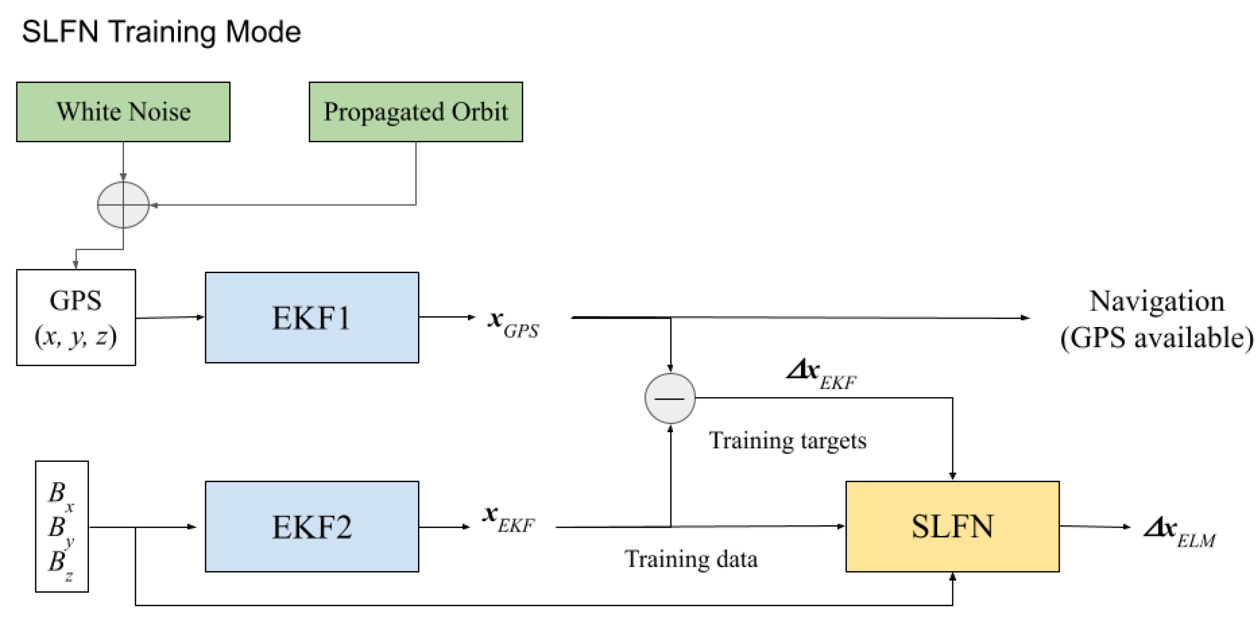
The algorithm was tested on the following scenario, assuming knowledge of the satellite’s attitude. This assumption was made to simulate the best possible performance of the EKF to further emphasize the improvement brought by the SLFN application. For six days, GPS data were available to the spacecraft as well as the state estimates provided by the magnetometer-based EKF. The first day of measurements was excluded from the training data in order to avoid data contamination due to the initial transitory phase of the EKF. The errors of each state estimate with respect to the state provided by the GPS-based EKF were sequentially computed and stored as training targets. After six days, the GPS was no longer available, the SLFN was trained using the stored data, and its prediction was used to perform orbit determination for the following 51 days of the run. The prediction scheme of the algorithm is shown in Figure 6.

The test was performed on the following hardware:

• CPU: AMD Ryzen Threadripper PRO 3975WX 32 Cores 3.50 GHz;
• RAM: 128 GB.

Table 5. ELM-trained SLFN and EKF performance comparison.

Algorithm	Average [Maximum] Position RSSE	Average [Maximum] Velocity RSSE
EKF (all)	$16.51$ [$31.83$] km	$2.07\times {10}^{-2}$ [$3.40\times {10}^{-2}$] km/s
SLFN (training)	$5.50$ [$13.20$] km	$6.32\times {10}^{-3}$ [$1.33\times {10}^{-2}$] km/s
SLFN (prediction)	$6.90$ [$19.70$] km	$8.76\times {10}^{-3}$ [$2.13\times {10}^{-2}$] km/s
	Standard Deviation (Position)	Standard Deviation (Velocity)
EKF (all)	$6.27$ km	$6.36\times {10}^{-3}$ km/s
SLFN (training)	$2.49$ km	$2.62\times {10}^{-3}$ km/s
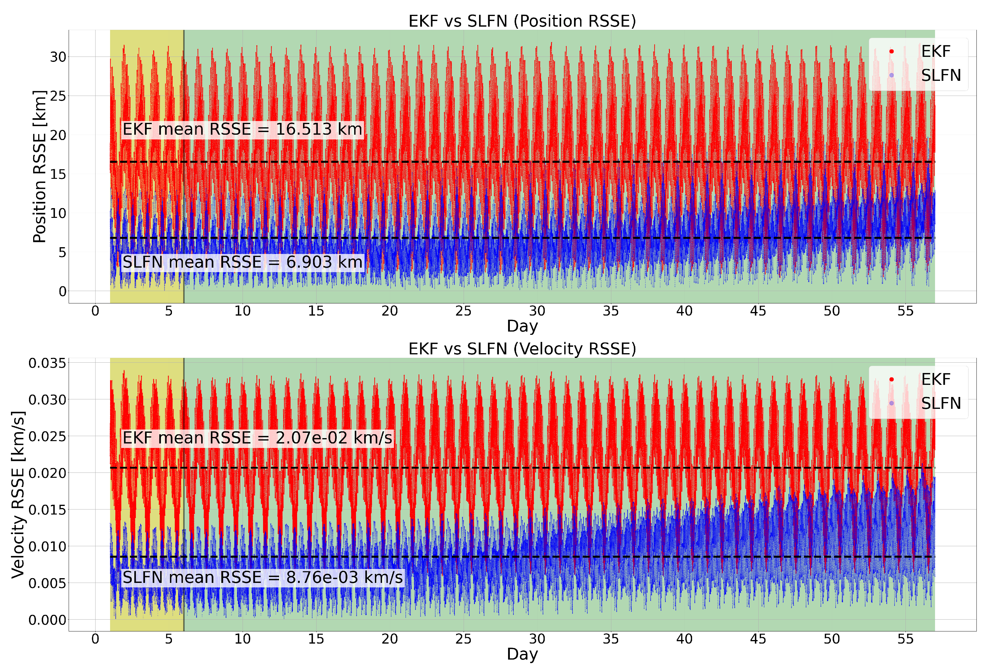
SLFN (prediction)	$3.04$ km	$3.72\times {10}^{-3}$ km/s

shows the comparison between the ELM-trained SLFN and the EKF in terms of the state RSSE and standard deviation. The training phase was carried out from the second to the sixth day, while the prediction phase went from the seventh days onwards. The error was computed with respect to the true propagated orbit. The prediction of the SLFN reduced the errors in the state estimate by a factor of 2.39 for the position and 2.36 for the velocity, with the respective mean RSSE decreasing from 16.51 km to 6.90 km and from $2.07\times {10}^{-2}$ km/s to $8.76\times {10}^{-3}$ km/s. Moreover, the sparseness of the RSSE was reduced by a factor of 2.06 for the position and 1.71 for the velocity. 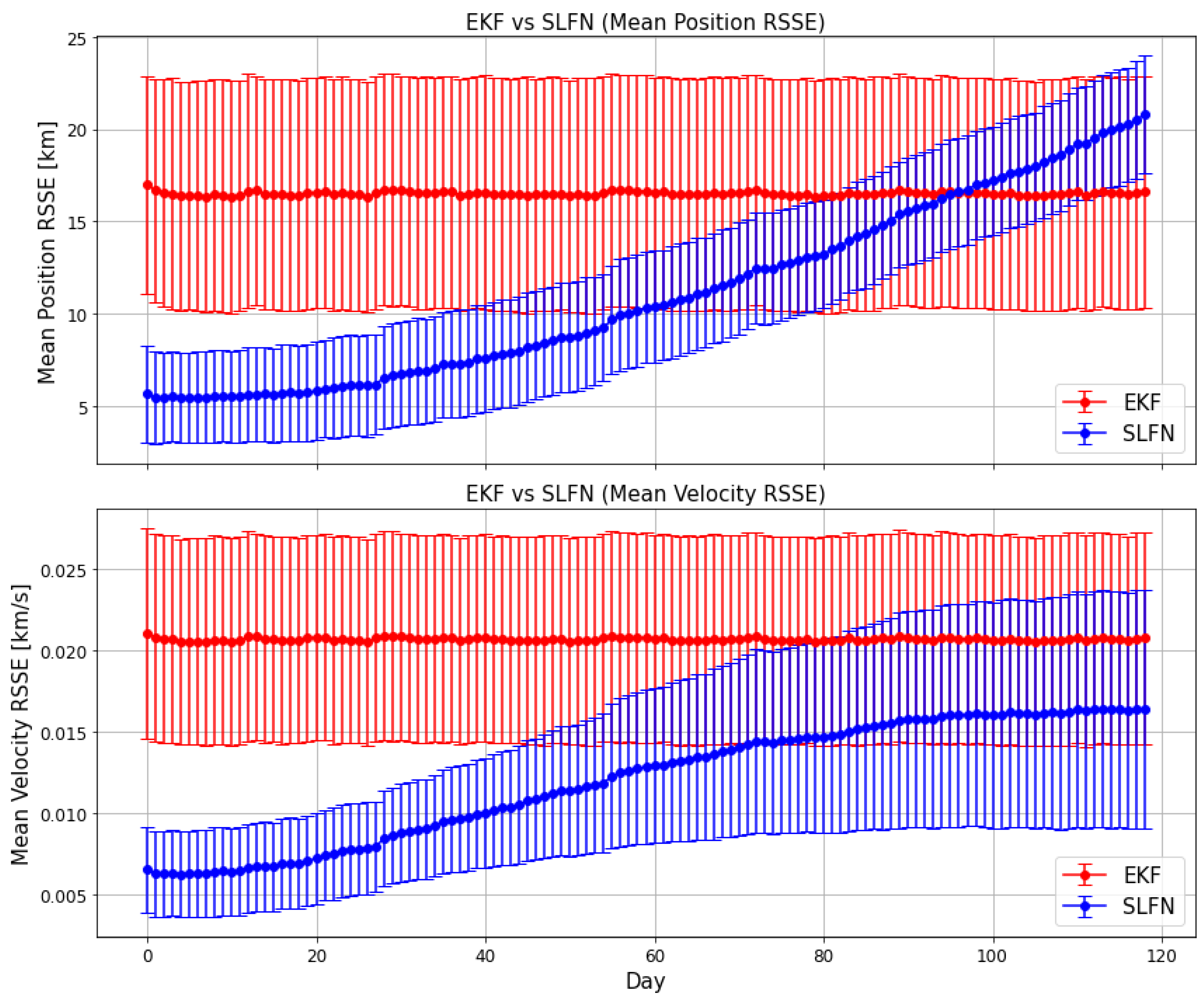Figure 7 shows the state RSSE over time. While the SLFN yielded a better state estimate than the EKF on average, the predictive capacity of the network started to decrease with time and could eventually lead to a divergence in the prediction. This was due to the fact that the SLFN was trained on an extremely small percentage of data and, in the long run, it struggled to handle never-seen-before data points given by the pseudo-periodic behavior of the orbit. This pseudo-periodic feature could also be seen in the RSSE as it showed a periodic trend itself, due to the difference between the real and simplified magnetic field models. A greater error in the state estimate corresponded to a region in which the discrepancy between the two models was deeper. An extended simulation of 120 days was carried out in order to study the behavior of the SLFN’s mean RSSE over time. Figure 8 shows the mean RSSE for both algorithms computed over each day of the simulation. While the position error clearly diverges, the velocity error stabilizes after approximately 100 days. Nonetheless, looking at the figure, it can be seen that the SLFN errors are inside the range determined by the EKF errors. Therefore, the SLFN approach yielded better or comparable results for up to 120 days. After this period, the SLFN did not represent an improvement over the EKF.

6. Discussion

The proposed algorithm reached kilometer- and meter-per-second-level accuracy in state estimation using a combined EKF-SLFN approach and the CHAOS-7 geomagnetic field model to simulate magnetometer measurements. The results obtained in this work, particularly in the performance of the EKF, were compared with the study conducted in [25], where a magnetometer-based EKF was applied to real flight data from four satellites with different altitudes and inclinations. This approach was justified by the discrepancy between the magnetic field models used in this work, which makes it closer to real data-based methods compared to the majority of cases where the onboard model and the measurement model are identical. Based on

Table 6. A comparison of the results between the EKF and SLFN in this work and the four case studies in [25] relative to the RXTE, ERBS, CGRO, and TOMS satellites.

Satellite	Inclination	Altitude	Avg. Position RSSE	Avg. Velocity RSSE
RXTE	23°	580 km	15 km	15 m/s
ERBS	57°	614 km	25 km	30 m/s
CGRO	28.5°	340 km	20 km	20 m/s
TOMS	97°	483 km	20 km	25 m/s
EKF (this work)	96.6°	567 km	17 km	21 m/s
SLFN (this work)	96.6°	567 km	6.90 km	8.76 m/s

, it can be observed that the accuracy of the EKF in this work, where magnetometer data were simulated using the CHAOS-7 model, is comparable to that achieved using real measurements. While this does not necessarily imply that the algorithm can be directly transferred to real data with the same level of accuracy, it highlights the validity of the CHAOS-7 model in simulating realistic magnetic field measurements.

7. Conclusions and Future Works

This work proposes an algorithm combining a magnetometer-based EKF with an ELM-trained SLFN to improve the accuracy of the EKF state estimate during GPS outages. A GPS-based EKF is used to provide ground truth values for the SLFN when GPS data are available, while the magnetometer-based EKF state estimate is used as the input of the SLFN. During GPS outages, the output of the SLFN is used to perform navigation. Magnetometer measurements are simulated using the CHAOS-7 geomagnetic field model. The SLFN was trained on GPS data with a five day-long availability window and tested on the following 51 days of GPS absence. Results for a simulated Sun-synchronous orbit showed an improvement of a factor of 2.4 in the spacecraft’s state estimate after the application of the SLFN, with the mean RSSE error decreasing from 16.51 km to 6.90 km for the position and from $2.07\times {10}^{-2}$ km/s to $8.76\times {10}^{-3}$ km/s for the velocity. Future steps in this direction involve the feasibility study of a direct onboard application of the presented algorithm. The main aspect to be considered is the memory required to store the training data that can exceed the capabilities small satellites. For this purpose, many subsequent trainings with small batches of data can be performed instead of a single, more demanding tuning of the output weights at the end of the GPS availability window. The Online Sequential Extreme Learning Machine (OS-ELM) [26,27] is a variant of the ELM specifically designed to update the output weights when a new batch of data is available in a sequential fashion. By performing so, the information relative to the previous batches can be deleted once the data are processed, significantly easing the computational stress on the algorithm. However, the optimal dimension of the batch must be determined empirically and meet the requirements in terms of both accuracy and computational burden. This issue can be tackled if the communication between the satellite and the ground station is available. The necessary data can be, in fact, transmitted to the ground station with a fixed frequency and then deleted from the satellite. The training of the network can be performed offline and the weights can be transmitted back to the satellite to be used if needed. Finally, this procedure permits the sequential updating of the weights if more GPS and EKF data are available, which could eventually solve the issue of a prediction losing precision and stability over time as a consequence of a single training performed on a small percentage of data at the beginning of the run. Another aspect to be taken into consideration is the required level of precision in the state estimate. Despite the improvement, the prediction may not be accurate enough for the requirements of the mission. This is mainly due to the baseline provided by the EKF estimate that has a mean RSSE of approximately 17 km and 21 m/s. A better baseline can be achieved by improving the geomagnetic model embedded in the EKF or, vice versa, simplifying the model used to simulate the magnetometer measurements. However, the former would inevitably increase the computational effort of the algorithm while the latter would not represent a realistic application in a real case. Furthermore, the main goal of this work was to test the behaviour of the EKF when the embedded model was a simplified version of the more accurate one used to generate the measurements. For this reason, future work will also investigate the use of an oversimplified model, such as a dipole approximation, onboard the EKF and its impact on the algorithms’s performance.

References

1. Pimienta-Penalver, A.; Linares, R.; Crassidis, J. Meeting orbit determination requirements for a small satellite mission. In Proceedings of the AAS/AIAA Space Flight Mechanics Meeting, Charleston, SC, USA, 29 January–2 February 2012. [Google Scholar]
2. Psiaki, M.L. Autonomous orbit and magnetic field determination using magnetometer and star sensor data. J. Guid. Control Dyn. 1995, 18, 584–592. [Google Scholar] [CrossRef]
3. Martel, F.; Pal, P.K.; Psiaki, M.L. Three-axis attitude determination via Kalman filtering of magnetometer data. In Proceedings of the NASA, Goddard Space Flight Center, Flight Mechanics (Estimation Theory Symposium 1988), Greenbelt, MD, USA, 10–11 May 1988. [Google Scholar]
4. Babcock, E. CubeSat Attitude Determination via Kalman Filtering of Magnetometer and Solar Cell Data. 2011. Available online: https://digitalcommons.usu.edu/smallsat/2011/all2011/56/ (accessed on 12 December 2022).
5. Kalman, R.E. A new approach to linear filtering and prediction problems. J. Basic Eng. 1960, 82, 35–45. [Google Scholar] [CrossRef]
6. Kalman, R.E.; Bucy, R.S. New results in linear filtering and prediction theory. J. Basic Eng. 1961, 83, 95–108. [Google Scholar] [CrossRef]
7. Kalman, R.E. New methods in Wiener filtering theory. In Proceedings of the First Symposium of Engineering Applications of Random Function Theory and Probability; Wiley: New York, NY, USA, 1963; pp. 270–388. [Google Scholar]
8. Psiaki, M.L.; Huang, L.; Fox, S.M. Ground tests of magnetometer-based autonomous navigation (MAGNAV) for low-earth-orbiting spacecraft. J. Guid. Control Dyn. 1993, 16, 206–214. [Google Scholar] [CrossRef]
9. Wiegand, M. Autonomous satellite navigation via Kalman filtering of magnetometer data. Acta Astronaut. 1996, 38, 395–403. [Google Scholar] [CrossRef]
10. Roh, K.M.; Park, S.Y.; Choi, K.H. Orbit determination using the geomagnetic field measurement via the unscented Kalman filter. J. Spacecr. Rockets 2007, 44, 246–253. [Google Scholar] [CrossRef]
11. Kim, S.; Petrunin, I.; Shin, H.S. A Review of Kalman Filter with Artificial Intelligence Techniques. In Proceedings of the 2022 Integrated Communication, Navigation and Surveillance Conference (ICNS), Dulles, VA, USA, 5–7 April 2022; pp. 1–12. [Google Scholar]
12. Gruber, M. An Approach to Target Tracking; MIT Lincoln Laboratory: Lexington, MA, USA, 1967. [Google Scholar]
13. Larson, R.E.; Dressler, R.M.; Ratner, R.S. Application of the Extended Kalman Filter to Ballistic Trajectory Estimation; Stanford Research Institute: Menlo Park, CA, USA, 1967. [Google Scholar]
14. Huang, G.B.; Chen, L.; Siew, C. Universal approximation using incremental constructive feedforward networks with random hidden nodes. IEEE Trans. Neural Netw. 2006, 14, 879–892. [Google Scholar] [CrossRef] [PubMed]
15. Huang, G.B.; Zhu, Q.Y.; Siew, C.K. Extreme learning machine: Theory and applications. Neurocomputing 2006, 70, 489–501. [Google Scholar] [CrossRef]
16. Finlay, C.C.; Kloss, C.; Olsen, N.; Hammer, M.D.; Tøffner-Clausen, L.; Grayver, A.; Kuvshinov, A. The CHAOS-7 geomagnetic field model and observed changes in the South Atlantic Anomaly. Earth Planets Space 2020, 72, 156. [Google Scholar] [CrossRef] [PubMed]
17. Alken, P.; Thébault, E.; Beggan, C.D.; Amit, H.; Aubert, J.; Baerenzung, J.; Bondar, T.; Brown, W.; Califf, S.; Chambodut, A.; et al. International geomagnetic reference field: The thirteenth generation. Earth Planets Space 2021, 73, 49. [Google Scholar] [CrossRef]
18. Zarchan, P.; Musoff, H.; Lu, F. Fundamentals of Kalman Filtering. A Practical Approach, 3rd ed.; AIAA: Reston, VA, USA, 2009. [Google Scholar]
19. Li, M.; Lei, Y.; Jiang, Q. An Attitude Control Scheme for Low Redundancy Micro-Nano Satellites without Gyroscopes. In Proceedings of the 2024 7th International Conference on Intelligent Robotics and Control Engineering (IRCE), Xi’an, China, 7–9 August 2024. [Google Scholar] [CrossRef]
20. Zhang, W.; Chen, Y.; Xue, G.; Lei, B.; Xia, Y.; Yu, X. On-Orbit Validation of OpenHarmony Real-Time Operating System Based on Dalian-1 Lianli Satellite. Space Sci. Technol. 2024. [Google Scholar] [CrossRef]
21. Akça, Ö.; Soken, H.E. Real-time Magnetometer Calibration and Misalignment Estimation for Small Satellites Using QUEST+ Kalman Filter Approach. In Proceedings of the 13th Nano-Satellite Symposium, Stellenbosch, South Africa, 25–29 November 2024. [Google Scholar]
22. Rodríguez, J.L.C. poliastro: A Python library for interactive astrodynamics. In Proceedings of the 21st Python in Science Conference, Austin, TX, USA, 11–17 July 2022. [Google Scholar]
23. Schmucker, U. Magnetic and electric fields due to electromagnetic induction by external sources. Landolt-Bornstein New-Ser. 1985, 5, 100–125. [Google Scholar]
24. Price, A. Electromagnetic induction within the earth. In International Geophysics; Elsevier: Amsterdam, The Netherlands, 1967; Volume 11, pp. 235–298. [Google Scholar]
25. Deutschmann, J.K.; Bar-Itzhack, I.Y. Evaluation of Attitude and Orbit Estimation Using Actual Earth Magnetic Field Data. J. Guid. Control Dyn. 2001, 24, 616–623. [Google Scholar] [CrossRef]
26. Ye, Y.; Squartini, S.; Piazza, F. Online sequential extreme learning machine in nonstationary environments. Neurocomputing 2013, 116, 94–101. [Google Scholar] [CrossRef]
27. Furfaro, R.; Barocco, R.; Linares, R.; Topputo, F.; Reddy, V.; Simo, J.; Le Corre, L. Modeling irregular small bodies gravity field via extreme learning machines and Bayesian optimization. Adv. Space Res. 2021, 67, 617–638. [Google Scholar] [CrossRef]
Figure 1. ELM Neural Network structure.
Aerospace 12 00117 g001
Figure 2. The tuning process of the measurement noise matrix R B = α 2 · I 3 × 3 . The position (left) and velocity (right) mean (blue) and maximum (red) RSSE of different EKF runs are shown against the corresponding value of R B . The best configuration is obtained for α = 1000 nT. Each EKF run has a duration of 100,000 s, corresponding to 10,000 iterations.
Aerospace 12 00117 g002
Figure 3. SLFN training process.
Aerospace 12 00117 g003
Figure 4. Locations of ground magnetic observatories providing data for derivation of CHAOS-7 from [16], published under license CC BY 4.0.
Aerospace 12 00117 g004
Figure 5. The geomagnetic field magnitude difference between the CHAOS-7 and IGRF-13 models at a fixed altitude of 567 km with a 5° resolution. The red line represents the satellite ground track from the beginning to the end of the simulation (from 3 January to 3 May 2019).
Aerospace 12 00117 g005
Figure 6. EKF-SLFN algorithm prediction scheme.
Aerospace 12 00117 g006
Figure 7. The EKF (red) and SLFN (blue) position (top) and velocity (bottom) RSSE over time. The yellow and green backgrounds distinguish between the training and prediction phases of the SLFN, respectively. The horizontal dashed lines correspond to the mean RSSE values over the whole run.
Aerospace 12 00117 g007
Figure 8. The daily EKF (red) and SLFN (blue) position (top) and velocity (bottom) mean RSSE over time, obtained from an extended 120-day simulation. Daily standard deviations are represented as error bars.
Aerospace 12 00117 g008