Digital Twin-Driven Design of an Ice Prediction Model

Abstract

This paper describes the development of an ice creation model to be used within the framework of a model-based systems engineering approach to predict the amount of ice growing on aircraft wings during flight. This model supports the preliminary design of the ice protection system, as well as the implementation of a control system, in real-time. When the aircraft meets a high concentration of super-cooled water in the atmosphere and a low temperature, the risk of ice formation on its external surfaces is significant. This causes a decrease in aerodynamic performance, with potential loss of control of the aircraft. To mitigate this effect, ice prevention and protection systems are crucial. The characteristics of the icing phenomena are first defined, then their effects on aircraft behavior during operation are evaluated. This allows us to develop a highly parametric predictive model of the actual icing conditions experienced by the aircraft during a given flight mission. To precisely predict the ice accretion and to design an ice protection system, estimating heat fluxes involving the aircraft’s wing surfaces and the external environment is required. To allow for this, this study also develops a thermal model that is specifically applied to the above-mentioned analysis. This model includes many factors characterizing the atmospheric conditions responsible for ice creation upon the aerodynamic surfaces, and it enables an accurate estimation and quantification of all the parameters necessary to design an appropriate ice protection system.

1. Introduction

Clouds with a high content of super-cooled water and low temperature are critical to aircraft flight, since the probability of ice formation on aerodynamic surfaces is very high. This phenomenon is a persistent challenge to aircraft safety because of its high potential to degrade aerodynamic performance and even affecting measurements during flight. When icing occurs on a wing, the change in airfoil shape decreases the lift and increases the drag, leading to potentially fatal accidents. Historical studies underscore the evolution of experimental and numerical research aimed at mitigating these risks, spanning from early icing physics experiments to sophisticated simulations that have been recently developed. In the 1970s, the development of numerical simulations for aircraft icing began [1]. Designing specific systems to either prevent or remove ice and to avoid flight problems associated with this phenomenon is necessary. Recent advances in aircraft safety emphasize the importance of accurately predicting ice formation. Unforeseen icing events have led to numerous flight incidents and accidents. Research has been conducted on airfoil aerodynamics under icing conditions, particularly over the period from 1978 to the present. This spans from the NASA (National Aeronautics and Space Administration) Lewis workshop, which initiated the modern research program on icing phenomena in aeronautics, to more recent developments following the ATR accident in 1994. A deeper analysis of aerodynamic performance in icing conditions has been performed by several researchers to properly predict aircraft safety [2].

Numerical simulations are widely used to perform these investigations [3]. Their cost-effectiveness ratio and capability of precisely modeling various systems of complex products have been effectively employed to predict and analyze the behavior and characteristics of ice formation. This also includes the possibility of simulating the influence that each system has on the others [4]. Thus, these kinds of models have the potential for a fairly accurate evaluation of ice accumulation. Several codes have been developed for simulating ice accretion, including LEWICE [5], CAPTA [6], TRAJICE2 [7], FENSAP-ICE [8], MULTIICE [9], and ICECREMO [10].

The first codes used to predict icing phenomena employed the Messinger [11] model. The ICECREMO code modeled the solidification of the run-back water film, which resulted in a wider applicability of this model to several icing conditions. More recently, Zhang et al. [12] included the effects of run-back water and the porosity of rime ice in the accretion process.

The model introduced in this paper aims to provide a simpler simulation and mathematical framework for analyzing these phenomena compared to some of the previously mentioned models. Despite its reduced complexity, our model is designed to deliver accurate predictions of ice accretion while ensuring compliance with the Certification Specifications for Large Aeroplanes (CS-25).

The framework developed in this work aims to support future extensions, specifically the integration of real-time data from sensors such as ice detection sensors (e.g., vibrating probes, optical or ultrasonic ice detectors), total air temperature (TAT) sensors, humidity sensors, angle of attack (AoA) sensors, Pitot-static sensors, infrared sensors, and others—aspects not addressed in this study due to its focus on digital models. The title refers to the digital twin-driven approach to the design of an ice prediction model, focusing on the development of a model that, through progressive iterations, aims to increasingly replicate the true physical behavior of the ice accretion phenomenon. The current model is merely a starting point. This predictive block represents a crucial initial step toward the development of a fully integrated digital twin, which will ultimately incorporate real-time sensor data to enhance the system’s predictive and diagnostic capabilities. Figure 1 below provides a block diagram to explain the logical functioning of the digital twin model.

The first section of this work investigates the physics and characteristics of icing phenomena related to in-flight aircrafts. The environmental conditions that lead to ice growth on the aerodynamic surfaces are included. The EASA (European Union Aviation Safety Agency) CS-25 Appendix C Certification [13] is then analyzed. This analysis allows us to draw a suitable workflow for a static ice thickness prediction. This model exploits input variables such as flight altitude, aircraft air speed, cloud extent, and the aircraft’s angle of attack. It provides an estimation of the icing formation experienced by the aircraft. The model is then used to investigate dynamic behavior, considering a demonstrative flight mission profile, with a random cloud distribution, aiming to evaluate the water impinging and ice thickness generated on the airframe during actual operation.

Before designing an anti-icing system, it is crucial to evaluate the local cooling phenomena occurring on the wing surfaces that lead to ice creation. This allows us to estimate the thermal contribution that the ice protection system must provide.

2. Icing Phenomenon and Cloud Characteristics

The creation of ice on aircraft surfaces, such as wings, ailerons, and engine intakes, occurs when the aircraft flies at an altitude where the temperature is either close or below the freezing point, and meets super-cooled water droplets. The extent and morphology of ice accumulation primarily depends on factors such as liquid water content, temperature, airspeed, droplet size, and surface roughness. Wind-tunnel and flight icing tests demonstrate that the presence of ice on unprotected aircraft components may give rise to several detrimental aerodynamic effects, thereby posing a significant safety concern. The most severe consequences include diminished maximum lift, heightened drag, reduced stall angle, alterations in pressure distribution, premature boundary layer transition, increased stall speed, and compromised controllability [14,15]. The ice accumulation on aircraft surfaces during flight is caused by cloud droplets retaining a liquid state despite sub-freezing temperatures. This phenomenon, also known as super-cooling, has a significant impact on the volume and characteristics of ice formation on aircraft elements. The most significant factors that can exert an influence on this process are reported in

Table 1. Factors influencing the increase or decrease of icing conditions.

	Factors Influencing Icing	Increase ↑ / Decrease ↓ Icing
Meteorological Characteristics	Low external air temperature	↑
	High amount of liquid water in the cloud	↑
	Increase of average size of the droplets	↑
	High airspeed	↑
	Increase of horizontal extent of supercooled cloud	↓
Aircraft Construction / Mission Type	Longer flight duration	↑
	Thicker wing profiles	↑
	Increase in the angle of incidence	↑
	Rougher surface finish	↑

.

Identifying the cloud type is fundamental for assessing icing phenomena. Clouds may be broadly classified into two types: stratiform (layer clouds) and cumuliform (clouds with vertical development), primarily based on altitude and horizontal extent, as shown in Figure 2.

In stratiform clouds, icing typically occurs at mid-to-low altitudes, i.e., below 3 km. These clouds are characterized by their stability and are approximately 2 km thick. High-level stratiform clouds (above 6 km), such as cirrus (Ci), cirrocumulus (Cc), and cirrostratus (Cs), are composed of ice crystals that can cause engine icing but generally do not lead to airframe icing. Flying through those clouds exposes the aircraft to prolonged icing conditions, which significantly influence the design of ice protection systems for some components, such as propellers and wings. Icing intensity in stratiform clouds varies from light to moderate, peaking in upper regions.

Cumuliform clouds, also known as convective clouds, play a significant role in the icing environment, because of their rapid growth, high liquid water content (LWC) and frequent supercooled state. They exhibit a vertical development with flat bases and occasionally flat tops, prevalent during fair weather conditions. They generally cover smaller areas, along the horizontal direction, when compared to stratiform clouds. Typically, those cloud formations span a relevant area, ranging from 3.7 to 11 km for an individual cloud. Icing intensity varies widely depending on cloud development stage, ranging from light in small cumulus clouds to severe in large cumulonimbus clouds. LWC can reach up to 2.5 g/m³, or even higher in tropical cumulonimbus clouds. Median droplet sizes typically range from 9 to 50 μm. Icing in these clouds results in clear ice or a mixture of clear and rime ice formations.

3. Predictive Model of Icing on Aircraft Wing

To develop a predictive model for assessing the icing conditions experienced by aircraft wings, the Appendix C in EASA CS-25 regulation is analyzed. This Appendix has been applied to extract icing-associated cloud parameters, such as LWC, MVD (Mean Volume Diameter) and environmental temperature, along with the relationships between these parameters.

3.1. Icing Maps Digitization

Within this regulation, a set of graphs is presented. Some depict continuous maximum icing conditions, associated with stratiform clouds, while others represent intermittent maximum icing conditions, i.e.,when the aircraft encounters cumuliform clouds. By utilizing software to digitize the graphs directly from their images, vectors can be extracted, each containing numerical data for MVD, LWC, and external temperature across all cloud types, including stratiform and cumuliform clouds with horizontal extensions ranging from 0.26 to 310 nmi. This process enables the generation of a 3D map (as shown in Figure 3) that includes all possible isotherms within the range of −30 °C to 0 °C, with a resolution of 0.25 °C. Such a fine temperature increment allows for a highly precise evaluation of LWC values corresponding to these isotherms.

This map enables the prediction of the LWC present in clouds encountered by the aircraft during a flight mission. This value is then used to calculate the water flux impacting the aircraft’s surfaces, providing an approximate estimate of the ice thickness that may form on them.

3.2. Calculation of Impinging Parameters

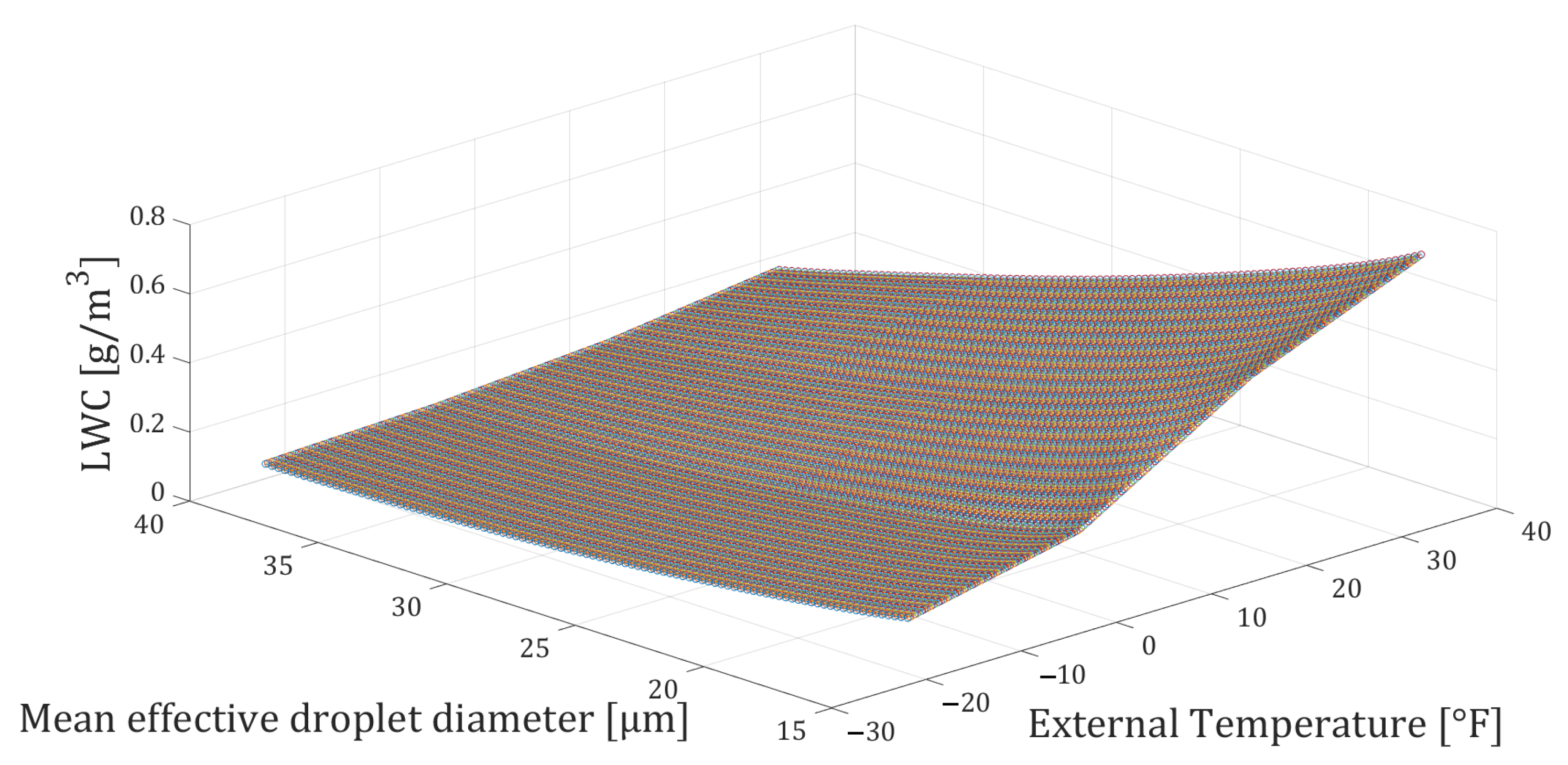
Supercooled clouds typically contain less than 1.0 g/m³ of liquid water in the air. This low concentration of water in the free-stream allows considering the particles present in that stream as they were uncoupled. Consequently, they have small impact upon the surrounding flow. When particles can be considered uncoupled, analyzing the overall flow as the sum of the individual contributions provided by each particle is possible. Moreover, the behavior of each particle can be studied separately by considering forces acting on it. Those contributions can be then summed to obtain a general identification of the whole flow.

In atmosphere, those droplets are typically less than 60 μm in diameter and can be approximated as spherical, because of their low Reynolds numbers. The trajectory of a single droplet approaching an object can be described by the following equation:

$$m{\displaystyle \frac{d^2\overrightarrow{x}}{d{t}^2}}=\overrightarrow{P}+\overrightarrow{M_a}+m\overrightarrow{g}+\overrightarrow{B}+\overrightarrow{D}$$

(1)

where m is the droplet mass, $d^2\overrightarrow{x}/d{t}^2$ is the droplet acceleration in approaching motion, and $\overrightarrow{P}$ and $\overrightarrow{M_a}$ are the pressure gradient and apparent mass, respectively (these terms are typically neglected because the density of the water droplet, i.e., the particle, is much greater than that of air, i.e., the fluid). In the above equation, $m\overrightarrow{g}$ represents the gravitational force, which can also be neglected due to the very small mass of supercooled water droplets. $\overrightarrow{B}$ denotes the Bassett (unsteady) “history” force: this term adjusts the drag factor for a sphere undergoing acceleration. The force $\overrightarrow{B}$ accounts for the modification in the flow pattern around the particle compared to the steady-state condition, capturing the influence of the particle’s motion history on the immediate force [15]. $\overrightarrow{D}$ is the drag force and the only factor that will be considered.

Equation (1) will then undergo a process to introduce non-dimensional parameters and incorporate the inertia K and the modified inertia $K_0$, as follows. Considering the vector $\overrightarrow{x}$, its components are x and y; their dimensionless values are defined as x* = x/c and y* = y/c, where c represents a characteristic length (in this application, the chord of the airfoil). The variables t and $V_{\infty }$ denote the time and free-stream airspeed, respectively. After appropriately reorganizing the equation, the following non-dimensional form is obtained:

$${\displaystyle \frac{d^2\overrightarrow{x^{*}}}{d{t}^2}}={\displaystyle \frac{1}{K}}{\displaystyle \frac{C_{D}Re}{24}}\left(\overrightarrow{u}-{\displaystyle \frac{d\overrightarrow{x^{*}}}{dt}}\right).$$

(2)

For simplicity, in subsequent equations, the asterisk will be omitted. As can be observed, the Reynolds number $Re$ and droplet inertia K are key parameters characterizing the trajectory equation.

The Reynolds number of the free-stream droplet is:

$$Re={\displaystyle \frac{{\rho }_a{V}_{\infty }\delta }{{\mu }_a}}$$

(3)

where ${\mu }_a$ is the air viscosity, and K is:

$$K={\displaystyle \frac{{\rho }_w{V}_{\infty }{\delta }^2}{18{\mu }_{a}c}}.$$

(4)

Applying the Langmuir and Blodgett theory [16], the variables $Re$ and K can be combined into a single parameter $K_0$, known as the modified inertia, which accounts for the influence of droplet size and, from a mathematical perspective, representing the Stokes number.

Furthermore, $K_0$ establishes a connection between droplet inertia and drag forces. When $K_0$ assumes small values, drag forces dominate, causing the droplet to align with the flow streamlines until it closely approaches the object impacted. When $K_0$ is sufficiently small (e.g., $K_0$ = 0.005), the droplet behaves as a flow tracer, following the fluid path. Conversely, higher values of $K_0$ indicate a predominance of droplet inertia, leading to a significant deviation from the flow streamlines as the droplet approaches the impacted object. When $K_0$ becomes notably large (e.g., $K_0$ = 1.0), the droplet trajectory becomes nearly linear, driven predominantly by its inertia. The mathematical expression of that parameter is:

$$K_0=18K\left[R{e}^{-{\displaystyle \frac{2}{3}}}-{\displaystyle \frac{\sqrt{6}}{Re}}arctan\left({\displaystyle \frac{R{e}^{\frac{1}{3}}}{\sqrt{6}}}\right)\right].$$

(5)

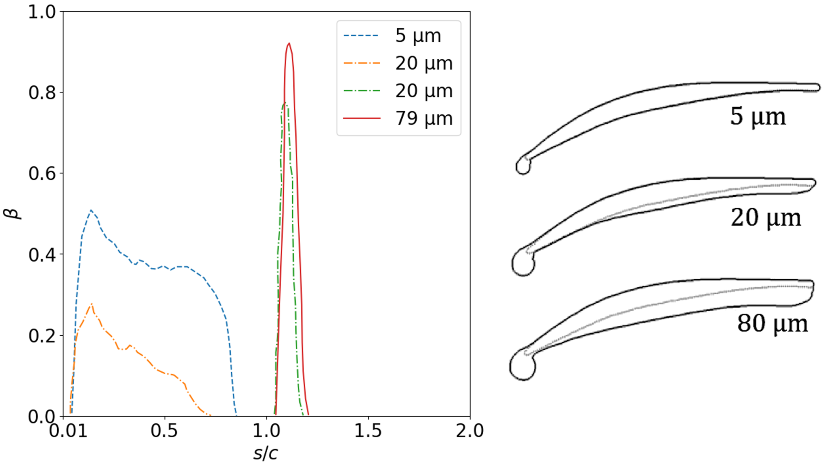
As the following results demonstrate, trajectories provide valuable insights into determining the mass flow rate of water impacting airfoils. The sensitivity of impact to droplet size is evident in Figure 4: on the left, the mass of water impacting the wing surface ($\beta$) peaks for larger droplet sizes, which is also observed on the right, where larger MVD results in larger ice formations. Peaks of enhanced impingement efficiency at the leading edge are particularly pronounced for larger droplet sizes (attributable to higher Stokes numbers). This phenomenon arises from the reduced inertia of smaller droplets, which causes them to follow the flow rather than collide with the wing surface. Conversely, scenarios with greater inertia lead to the development of larger ice formations, characterized by a more pronounced downward growth trajectory. This descent is further amplified by incoming droplets casting shadows on the region behind the leading edge [17].

As evident in Equations (3)–(5), calculating $Re$, K, and $K_0$ requires knowledge of certain atmospheric parameters related to altitude, such as temperature, density and viscosity of the air. To this end, data from the International Standard Atmosphere (ISA) have been utilized. ISA represents a static model of Earth’s atmospheric variations, including pressure, temperature, density, and viscosity across a broad range of altitudes. The ISA is endorsed as a global standard by the International Organization for Standardization (ISO) under ISO 2533:1975. The model starts at a base geo-potential altitude of 610 meters (2000 ft) below sea level, with standard temperature set at 19 °C [18], as shown in Figure 5.

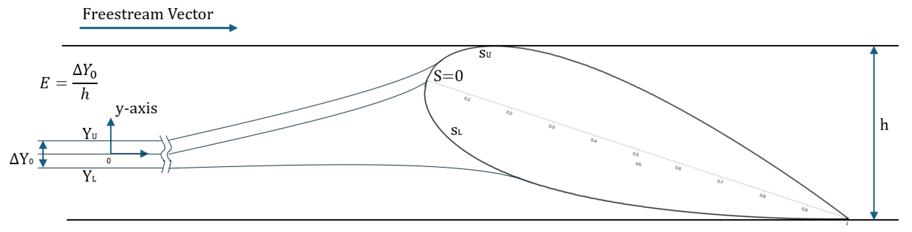
Another important parameter to analyse the trajectory of droplet is the total impingement (or collection) efficiency E, i.e., the ratio between the free-stream impingement width ${\Delta }_{Y0}$ and the projected frontal height h:

$$E={\displaystyle \frac{{\Delta }_{Y0}}{h}}$$

(6)

As described in Figure 6, E represents the fraction of liquid mass that crosses the Y axis within the frontal projection of the airfoil and subsequently impinges upon the airfoil surface. To make those values dimensionless, they are divided by the chord length. The non-dimensional parameter ${\Delta }_{Y0}$ visualizes a segment along the Y axis with a length equivalent to one chord, centered at the projected location of the airfoil leading edge. ${\Delta }_{Y0}$ represents the portion of liquid mass that crosses the Y axis within this segment and eventually interacts with the airfoil.

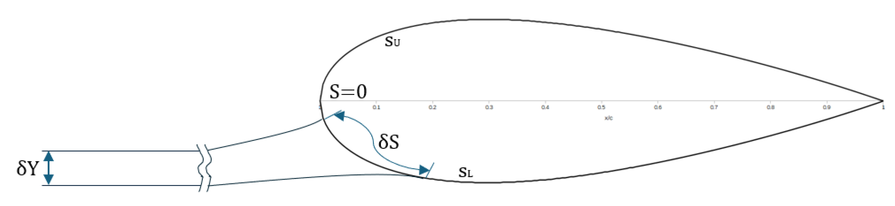
The last fundamental parameter is $\beta$, being the local (or collection) efficiency. It is calculated at a chosen point P along the airfoil. Considering point P as the location where two droplet paths intersect the airfoil surface, $\beta$ represents the concentration factor, i.e. the local impact efficiency on a small portion of the wing profile. As observed in Figure 7, it corresponds to the mass of water present between the two free-stream trajectories, denoted as ${\delta }_{Y0}$, that impacts the surface of the wing profile identified by ${\delta }_S$:

$$\beta =\underset{x\to 0}{lim}{\displaystyle \frac{{\delta }_{Y0}}{{\delta }_S}}={\displaystyle \frac{d_{Y0}}{d_S}}.$$

(7)

The maximum value assumed by $\beta$ on the airfoil surface is ${\beta }_{max}$. It is maximum for symmetrical surfaces and corresponds to the limit value for an infinitesimal part of the wing area concentrated in the stagnation point. The function of this parameter will be clarified in Section 4.2, where it will be extensively used.

To implement this model, the following assumptions have been introduced:

• Values of temperature, density, and air viscosity, according to ISA;
• Profile of wings selected is the NACA 0012 with the following characteristics: chord = 3 m, wingspan = 15 m, metal sheet thickness = 3 mm; NACA stands for National Advisory Committee for Aeronautics. The Profile 0012 has symmetrical airfoil with a thickness 12% of the chord value.
• The MVD is set at 20 μm, as suggested by the conventions in the scientific literature for evaluating ice accretion [13];
• Angle of attack of aircraft assumed equal to pitch angle.

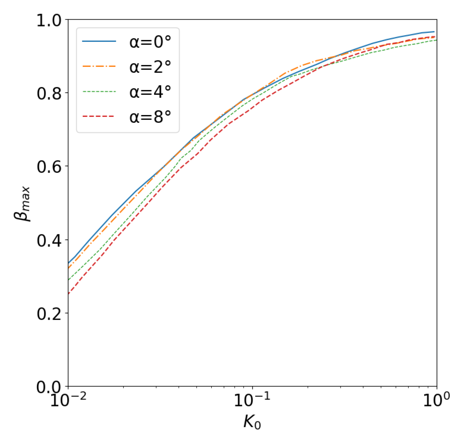
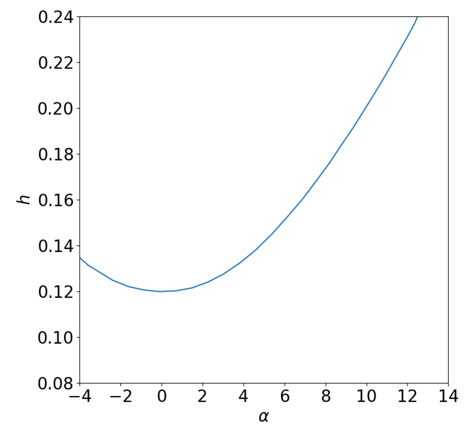
NACA has drawn several charts that allow for a highly accurate estimation of the E, ${\beta }_{max}$, and h values for different angles of attack $\alpha$ and the modified inertia parameter $K_0$. These values can be obtained through the use of Figure 8, Figure 9 and Figure 10, which have been digitized and subsequently interpolated to generate numerical maps, as was done with LWC in Section 3.1 [15,19,20,21,22,23,24].

3.3. Model for Ice Accretion Prediction

Once all relevant variables required for the quantitative analysis of the icing phenomenon have been obtained, it is possible to proceed with the modeling of the phenomenon. The first part of the model consists of a script developed in MATLAB^®, which, taking as inputs: flight altitude (in ft), aircraft velocity (in kt), cloud extent (in nmi), and aircraft angle of attack (in degrees), allows obtaining the following information for a specific moment during the flight mission:

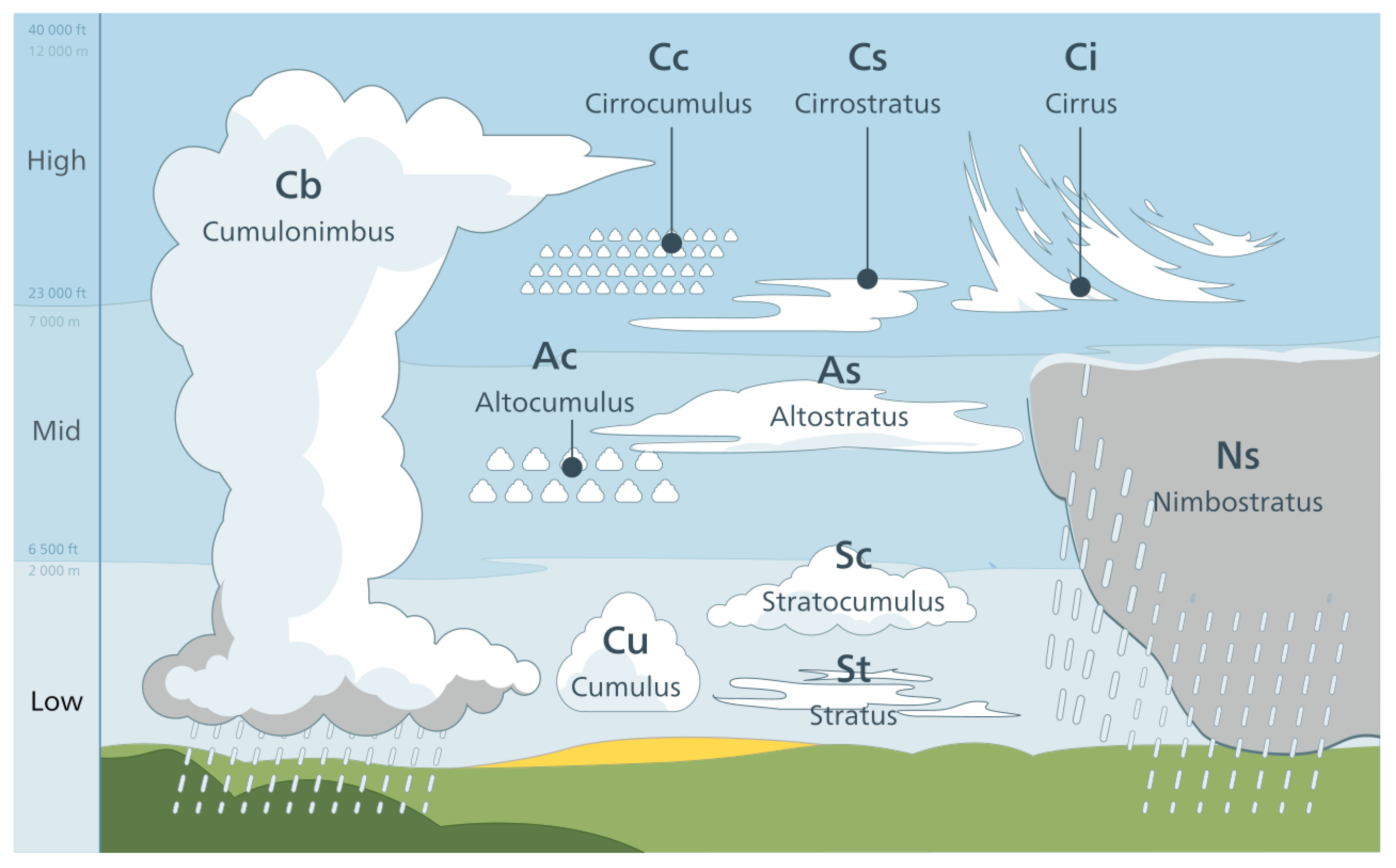
• Type of cloud encountered, based on the horizontal extent of the cloud encountered during the flight;
• Type of ice accretion, dependent on the cloud type: intermittent if a cumuliform cloud is encountered, otherwise continuous for stratiform clouds;
• The mass flow rate of water due to the LWC present in the cloud that collides with the wing surface, expressed in kg/s $·$ span;
• The thickness of ice accumulated on the wings, in mm.

To predict the ice thickness, the water impingement rate ṁ (kg/s $·$ span) is calculated as:

$$\dot{m}=1.568\times {10}^{-4}·V_{\infty }·LWC·E·h·c$$

(8)

where c is the wing chord (in ft), $V_{\infty }$ is the free stream velocity (in kt), h is the projection of wing height depending on the angle of attack (dimensionless when divided by the chord value) obtainable from Figure 10, E is the total impingement (or collection) efficiency (dimensionless), and LWC is the liquid water content (in g/m³). The ṁ value should be multiplied by the wing span extension (in m) to obtain the contribution to the entire airfoil.

To evaluate the thickness of the ice accretion, the accumulation parameter $A_C$ is calculated as:

$$A_C=1.0131\times {10}^{-4}{\displaystyle \frac{LWC·V_{\infty }·r}{{\rho }_{ice}·c}}$$

(9)

where r is the time of flying in cloud expressed in minutes, and ${\rho }_{ice}$ is the ice density assumed as rime ice = 0.8 g/cm³ [25].

Assuming that ice growth is orthogonal to surface, the maximum ice thickness (in mm) in chord is, as in [15]:

$$l_{max}=3.048\times {10}^2·A_C·{\beta }_{max}·c$$

(10)

It should be noted that the assumptions and results presented in this study are specifically valid for very small ice thicknesses. The applicability of these findings to larger ice accretions has not been verified and may require further investigation or modifications to the model.

In Figure 11 the algorithm that summarizes the functional steps of the proposed model is reported.

3.4. Validation of the Model

To validate the above described model, a comparison has been carried out with the experimental results published by the NASA Lewis Research Center (LeRC) and performed at the Icing Research Tunnel (IRT) [26]. To test our model, we provided the same input parameters that lead to ice formation as used in the NASA article, and the results were compared with the experimental data presented in the cited study.

The airfoil used in the NASA experiment is the NACA 0012, the same previously exploited; the chord is set to 21 in. In

Table 2. Experimental setup parameters of the NASA study.

Test Cases	$\mathit{\alpha }$ [deg]	Freestream Velocity ${\mathit{V}}_{\mathit{\infty }}$ [mph]	LWC [g/m3]	MVD [μm]	Exposure Time to Icing Conditions [Minutes]	Total Temperature [°C]
Case 1	4	150	1	20	6	−26
Case 2	4	230	0.55	20	7	−11
Case 3	4	230	1	30	6	−5
Case 4	4	150	1	20	6	−2

, the setup values of test cases proposed by the NASA study are reported, while in

Table 3. Results comparison between the NASA study and the proposed model. The values are dimensionless as they represent the maximum ice thickness relative to the chord length, x/c.

Case	Results of the NASA Study (Benchmark)	Results Obtained with the Proposed Model by Imposing the LWC from the NASA Study	Percentage Variation from the Benchmark	Results Obtained with the Proposed Model with Computed LWC	Percentage Variation from the Benchmark	Ice Shape
1	0.025	0.038	52%	0.0066	−73.6%	Rounded
2	0.025	0.041	64%	0.0252	0.8%	Rounded
3	0.025	0.0738	195.2%	0.0191	−23.6%	Horned
4	0.025	0.038	52%	0.0232	−7.2%	Horned/rounded

are shown the results obtained by the IRT alongside the proposed model’s.

The tests are conducted in two different ways, differing in the input value of LWC. In the first test, the LWC is provided as in the NASA study, while in the second method, the LWC is calculated according to the model based on Appendix C in EASA CS 25 described above.

In most cases, the ice thickness prediction performed by the model shows results comparable to the experimental ones. Particularly, better results are found for Cases 2, 3 and 4 in Table 3. Values obtained computing the LWC values according to the CS 25, are quite close to those found in the wind tunnel. The differences in the results are more pronounced when the LWC value, as considered in the icing conditions proposed in the NASA study, is imposed on our model.

Slight discrepancies have been observed between model predictions and experimental results, being related to some assumptions and simplifications, but the overall consistency of model predictions demonstrates robustness and reliability. Differences (as in Case 1) could be associated to the LWC calculated without defining the cloud extent, being only estimated through flight time and cruise speed. This might turn out into an inaccuracy in the identification of cloud type. Moreover, the EASA model replicates physical conditions upon statistical approach, but is incapable of replicating every atmospheric condition. In Case 1, with a MVD of 20 μm and a temperature of $-26$ °C, the CS 25 Appendix C provides a LWC of 0.4, considering stratiform clouds, while in the NASA experiments, the value is set to 1.

Another critical issue could be the time required to cross a cloud. In this model, when the aircraft encounters a cloud, it passes through it along its horizontal extension, and the crossing time is determined by its current speed. Crossing times may differ from those proposed in the NASA paper. Therefore, if LWC is imposed on the model without providing precise information on the cloud’s horizontal extension, the calculated crossing time may differ from those used in the NASA tests.

Ice thickness calculated by setting the value of LWC according to the proposed model, might be slightly overestimated, especially when cruise speed and temperature are increased and MVD is decreased (high altitudes are characterized by low temperatures and MVD). Humidity (represented by the MVD parameter) is high at middle-lower altitudes because temperatures are less severe. Furthermore, the equation enabling assessment of water impingement rate and maximum ice accretion thickness is an approximation. Firstly, it relies on free stream and statistical atmospheric parameters. Secondly, the impingement parameters are developed based on an uncontaminated surface. As ice accumulates, the resulting body’s shape evolves, impacting the flow dynamics and impingement parameters. For instance, under prolonged glaze conditions, a substantial glaze ice shape could indeed form, leading to insufficient approximations with some of the presented equations [15].

More precise outcomes are attainable only through the use of CFD (Computational Fluid Dynamics) analyses on surfaces exposed to icing. Nevertheless, the model here presented allows finding results comparable to experimental evidences. It requires significantly fewer computational and time resources compared to CFD simulations and proves effective in generating reasonably overestimated values.

Therefore, despite an evident approximation, the proposed model has been validated, and it may prove useful in the design of icing prevention systems. Such is particularly true during conceptual and preliminary system design, where the necessity to test multiple solutions requires fast and easily executable models and, in order to cover most operational scenarios, overestimated results can be advantageous.

4. Implementation of the Icing Prediction Model in Dynamic Conditions

In this section, ice formation on the aircraft surfaces is applied to a flight mission, characterized by various types and extents of cloud coverage that evolve continuously throughout the flight. The model is parametric and adaptable to different scenarios, allowing for easy replacement with new information regarding the flight mission and cloud types.

4.1. Cloudy Flight Mission

A first extension of the model depicted in Section 3.3 consists in incorporating the information about the mission profile. So, the model is exploited to predict ice thickness and water impingement on wings over the entire flight path. The external temperature, pressure, density and viscosity of the air are evaluated consistently with the ISA model.

Table 4. Table of flight mission parameters.

Flight Mission Completion [%]	Altitude [% w.r.t. Maximum Quota]	Angle of Attack [°]	Velocity [% w.r.t. Maximum Velocity]	Phase of Flight Mission
0	5	2.24	88	start climb
6	100	2.24	88	end climb
6	100	0	95	start cruise
75	100	0	95	end cruise
75	100	1.79	100	start descend
82	5	1.79	100	end descend
82	5	0	55	start loiter
100	5	0	55	end loiter

shows the dimensionless flight mission parameters assumed for the present work.

The cloud conditions and flight path are described in

Table 5. Table of cloud structures over flight mission.

Phase of Flight	Type of Cloud Encounter	Horizontal Extent [nmi]
Climb	cumuliform clouds	3
Cruise	stratiform cloud	100
Descent	cumuliform clouds	4
Loiter	stratiform cloud	40

and Figure 12. The cloud profile has been designed to set up a demonstration aiming at representing complex and challenging icing conditions. This approach allows for a better assessment of the ice protection system’s performance under difficult scenarios. To this end, the descent and climb phases—typically the most demanding in terms of aircraft performance—encounters with cumuliform clouds, which exhibit higher LWC values [27] creating more complex flight conditions, were prioritized. This choice ensures a more significant presence of icing, enabling the evaluation of an anti-icing system that is conservative and robust, accounting for even the most severe conditions.

4.2. The Mass Flow Rate of Water Impingement

To make the model more accurate, it is useful to improve the calculation of water flow impacting the airfoil profile by using a model that better fits the real behavior of droplet distribution in the cloud. A possible solution can be to resort to the Langmuir and Blodgett model [16].

The rate of water impact at any given point results from summing up the rates of impact for the volume of water encompassed within each droplet size. The mass flow rate of water impingement could be calculated at any point on the surface as:

$$M_a=V·\mathsf{\Sigma }\left(n·\beta \right)$$

(11)

where $\beta$ is the collection efficiency (concentration factor, seen in Equation (7)) for a particular value of the drop inertia K (see Equation (4)), and n is the concentration of liquid water contained in drops of a particular size.

According to Langmuir’s theory, the E-type drop-size distribution, reported in

Table 6. Table of statistical water distribution in cloud. s/c indicates the non-dimensionalization of the aircraft wing profile projected onto the wing chord; for instance, “2% of s/c” signifies that we are at the point on the surface corresponding to 2% of the wing chord length. A cruise condition is considered, where there is symmetry of water distribution on the wing.

E droplet distribution	0.23	0.44	0.65	1	1.45	2	2.71
n/LWC	0.05	0.1	0.2	0.3	0.2	0.1	0.05
n	$2.54\times {10}^{-7}$	$5.08\times {10}^{-7}$	$1.02\times {10}^{-6}$	$1.52\times {10}^{-6}$	$1.02\times {10}^{-6}$	$5.08\times {10}^{-7}$	$2.54\times {10}^{-7}$
s/c	$\beta$							$M_a$ [lbm/h$ft$]	$M_a$ [kg/s ft]
0	0.250	0.350	0.380	0.480	0.630	0.730	0.810	4.865845807	$6.13\times {10}^{-5}$
0.1	0.15	0.34	0.37	0.48	0.630	0.730	0.8	4.784268511	$6.03\times {10}^{-5}$
0.2	0	0.31	0.37	0.47	0.630	0.72	0.79	4.640308576	$5.85\times {10}^{-5}$
0.5	0	0.15	0.32	0.45	0.6	0.71	0.77	4.256415415	$5.36\times {10}^{-5}$
0.7	0	0	0.28	0.42	0.58	0.69	0.75	3.882119584	$4.89\times {10}^{-5}$
1	0	0	0.15	0.38	0.54	0.65	0.71	3.383058475	$4.26\times {10}^{-5}$
1.4	0	0	0	0.3	0.47	0.59	0.67	2.653661471	$3.34\times {10}^{-5}$
2	0	0	0	0.14	0.35	0.49	0.57	1.818693847	$2.29\times {10}^{-5}$
2.4	0	0	0	0	0.27	0.42	0.51	1.166075475	$1.47\times {10}^{-5}$
3	0	0	0	0	0.15	0.33	0.43	0.810974301	$1.02\times {10}^{-5}$
4	0	0	0	0	0	0.2	0.32	0.345503844	$4.35\times {10}^{-6}$
6.5	0	0	0	0	0	0	0.14	0.067181303	$8.46\times {10}^{-7}$
10.8	0	0	0	0	0	0	0	0	$0.00\times {10}^0$

, is assumed, which could lead to more substantial ice formation because it shows the highest amount of LWC and the largest MVD. Knowing the LWC value, it is possible to calculate n, starting from n/ LWC quotient and performing the inverse calculation.

As explained by Equation (11), to calculate $M_a$ it is necessary to sum the products of $\beta$ and n for any E distribution value of droplet in cloud and then, multiply it by the velocity. For example, the distribution of water impinging detected during the cruise phase of the flight mission considered in the previous section is reported in Table 6. In this phase of flight the LWC corresponds to 0.081 kg/m³ (equivalent to 5.08 $\times {10}^{-6}$ pounds/ft³) and the velocity is 1.889 $\times {10}^6$ ft/h.

As Table 6 shows, $M_a$ is distributed along the wing chord, and it is furthermore evaluated along a single section of the wing profile. To find the overall mass flow rate of water impingement, $M_S$, it is required to sum the contributions of each section. The NACA 0012 is symmetrical, therefore it is sufficient to find $M_a$ for only one of those sections, multiply by the wing length, and doubling the result, to consider the upper and lower parts of the airfoil.

As in Figure 13, the distribution of the water impinging rate is uneven along the surface. The highest water load is applied to leading edge, $s/c=0\%$, being the most exposed part to the fluid. This value is null at 10.8% of the chord length.

The water interception area is determined by the largest droplets present in the cloud. In case of E-type drop-size distribution, the largest drops are 2.71 times larger than the mean-effective diameter of the droplet (see Table 6 first row). Therefore, considering $MVD=25$ μm, the maximum drop diameter is 2.71 × 25 = 68 μm.

The maximum K value found during simulation in the previous section is around 0.47. Since it is the highest value, it induces the highest value of E as well, and a larger intensity of water impinging [28]. In Figure 14, $K=0.47$ corresponds to an efficiency of impingement E of 54%.

Considering Equation (6) it follows:

$$y_{0,limit}=Eh$$

(12)

and $h=y_{max}$ for the NACA 0012 airfoil corresponds to 12%. Code “0012” indicates a specific type of airfoil, with the following characteristics: the first two digits “00” stand for symmetrical, i.e., it has no camber, the last two digits “12” suggest that the maximum thickness of the airfoil occurs at 12% of the chord length.

Dividing both terms by the chord value c it follows:

$${\displaystyle \frac{y_{0,limit}}{c}}=E{\displaystyle \frac{h}{c}}$$

(13)

and

$${\displaystyle \frac{y_{0,limit}}{c}}=0.54\times {\displaystyle \frac{0.12}{2}}=0.032=3.2\%$$

(14)

Height h is also divided by 2, considering only the upper part of airfoil. Looking at the blue curve in Figure 15, the impingement area was found to be $10.8\%s/c$; beyond this value of $s/c$ no drops will occur.

The last deduction made for the NACA 0012 indicates that the area affected by the water impinging extends up to 10.8% of the chord length. Therefore, in the following sections, only this portion of airfoil surface will be examined, to study the icing phenomenon.

4.3. Results Obtained

Integrating the previously calculated $M_S$ with the cloudy flight mission of Figure 12, the water impingement along the entire flight path is found, as shown in Figure 16.

During the phases of cumuliform clouds crossing (as observed during climb and descent), there is a significant increase in water impingement, leading to an amplified ice accretion, as shown in Figure 17.

This effect is confirmed in Figure 18, which shows the cumulative ice growth without the intervention of any ice protection systems. Within the 0–5% of flight mission, the ice formation increases by approximately 4 cm, while during cruise (which accounts for about 60% of the whole mission) there is another increment of 4 cm, spread over a time span 11 times longer than the climbing phase. A similar trend is observed during the descent, which has a duration comparable to that of the climb, where the ice thickness increases by nearly 5.5 cm. This behavior can be explained by the fact that ascent and descent are typically characterized by atmospheric conditions with middle-lower temperatures (from $-10$ °C to 0 °C) and consequently clouds show higher humidity. This phenomenon is further emphasized by the presence of cumuliform clouds, which inherently have higher LWC compared to stratiform clouds. By configuring the flight mission in this manner, a worst-case scenario has been considered.

It is important to note that aircraft crosses cumuliform clouds quite fast, but humidity content is intense, whereas flying through stratiform clouds is longer-lasting, but they have lower LWC. Based on those results, it is crucial to understand how to adjust an ice protection system to withstand extreme environmental conditions.

5. Thermal Analysis of Wing Surfaces

Once a model to predict ice formation has been developed, for a precise sizing of the ice protection system it is fundamental to have a thermal model, enabling the prediction of heat exchanges occurring between the wing surface and the external environment. Thermal analysis is here performed to identify the amount of heat lost from wing surfaces during the same flight mission with clouds coverage previously discussed. To perform this analysis the knowledge of water impingement rate is fundamental (see Figure 16).

During flight in icing conditions, a wing experiences cooling due to convective heat transfer, water evaporation from its surface and the impact of water droplets, particularly in the droplet interception area (see Figure 19). Consequently, the amount of heat that is removed from the wing surface depends on the magnitude of convection, evaporation and conduction caused by water impingement rates. The unit heat q involved in the heat balance on a partially or completely wet surface, exposed to icing condition in terms of heat flux in W (see Figure 20), is evaluated as:

$$q=q_w+q_c+q_e$$

(15)

where $q_w$ is the heat exchanged due to warming of the intercepted water, $q_c$ is the heat exchanged due to forced convection, and $q_e$ is the heat exchanged due to the evaporation of the impinging water.

Furthermore, the heat flux q indicates the heating power that the ice preventing system must provide to counterbalance the heat losses from the wings surface.

5.1. Heat Exchanged Due to Warming the Intercepted Water

In case of flight, the impact process between the wing surface and moisture particles involves the exchange of dissipative forces such as friction, leading to a thermal flux that causes wing heating. The heat flux $q_w$ caused by such impact on the wing can be calculated as:

$$q_w=c_{pwater}{M}_a\left[t_s-\left(t_0+\Delta t_{kw}\right)\right]$$

(16)

where $c_{pwater}$ is the specific heat coefficient of water, $M_a$ is the flow of water impinging, $t_s$ is the temperature of the airfoil surface, $t_0$ is the temperature of the free-stream conditions. $\Delta t_{kw}$ is the kinetic temperature rise of water caused by stoppage of droplets as they strike the wing, being computed as:

$$\Delta t_{kw}={\displaystyle \frac{V^2}{2gJ{c}_{pwater}}}\approx 2°\mathrm{F}$$

(17)

where V is the free-stream velocity (in ft/s), g is the acceleration of gravity (equal to 32.2 ft/$s^2$), and J is the mechanical equivalent of heat (equal to 778 ft$·$lbs/BTU). Since in almost all cases $\Delta t_{kw}<2$ °F, for the following calculations it has been neglected.

Considering the same flight and environmental conditions shown in Figure 13, the corresponding graph of the heat flux $q_w$ caused by the water droplets impacting the wing can be seen in Figure 21. In this case as well, it is evident that heating is required for up to 10.8% of the surface relative to the chord, and the area most affected by the impingement phenomenon is at the point where s/c = 0%, with cooling gradually decreasing until it ceases at the 10.8% point.

In accordance to [30], a suitable design criterion for ensuring ice prevention is keeping the heated surfaces approximately 100 °C higher than the ambient air temperature during flight. Consequently, for the scope of this analysis, it is imposed a minimum temperature increase of about 100 °C across all points of the wing and aerodynamic surfaces located between 0 and 10.8 % of the chord length.

Considering the heat exchange due to the intercepted water over the entire flight mission, we obtain the result shown in Figure 22.

5.2. Heat Exchanged Due to Forced Convection

When a wing moves through the air, its surface temperature becomes higher than that of surrounding ambient temperature, because of frictional forces applied by the air.

The heat transfer rate per unit area from the surface of a body in an airflow caused by convective heat transfer is:

$$q_c=h\left(t_s-t_{0k}\right)$$

(18)

where h is the convective heat-transfer coefficient, which can be evaluated by measurements in clear air (in BTU/h °F ft²) and obtained from Figure 23, and $t_{0k}=t_0+\Delta t_k$ is the clear-air kinetic-temperature. $\Delta t_k$ represents the required increase in temperature for the surfaces to reach the desired temperature $t_S$.

Transition from laminar to turbulent flow over the airfoil surfaces was assumed to occur at the point of laminar separation. In all instances, the separation point was located considerably downstream of the heated region. The literature suggests that the boundary layer remains laminar over the heated areas [30]. Therefore, if one considers only the surface between 0 and 10.8% of the chord, $t_{0k}$ can be calculated according to the following [28]:

$$t_{0k}=t_0+{\displaystyle \frac{V^2}{2gJ{c}_{pwater}}}·\left[1-{\displaystyle \frac{U^2}{V^2}}·\left(1-P{r}^{1/2}\right)\right]·{\displaystyle \frac{{\alpha }_s}{{\alpha }_d}}$$

(19)

where U is the local velocity just outside the boundary layer (in ft/s), $Pr$ is the Prandtl number, ${\alpha }_s/{\alpha }_d$ is the ratio of the wet- to dry-adiabatic lapse rates, which can be obtained from Figure 24, and $U^2/V^2·\left(1-P{r}^{1/2}\right)$ is the recovery factor for NACA 0012 airfoil which can be evaluated from Figure 25.

Figure 26 describes the convective heat transfer value $q_c$ evaluated on the entire flight mission. In this case, the trend differs from the other heat fluxes, as it is not correlated with the LWC parameter, but rather with the friction forces applied by the air flow on the airfoil.

5.3. Heat Exchanged Due to Evaporation of Impinging Water

The amount of heat coming from a wet surface as a result of the evaporation of water impinging can be expressed as:

$$q_e=h\left(X-1\right)\left(t_S-t_{0k}\right)$$

(20)

where $t_s$ is the surface temperature, $t_{0k}$ is the clear-air kinetic temperature, and X is the evaporation factor.

The evaporation factor applies exclusively when the surface is entirely wet. In case of partial wetness, the value of X should be adjusted based on the extent of the wet area, and it can be evaluated as:

$$X=1+3.75\left({\displaystyle \frac{e_s-e_{0k}}{t_S-t_{0k}}}\right)·{\displaystyle \frac{P_{SL}}{P_l}}$$

(21)

where $P_{SL}$ is the standard sea-level pressure (assumed to be 760 mmHg), $P_l$ is the local static pressure (obtained from the ISA model, in mmHg), and e is the saturation vapor pressure with respect to water, computed with the Antoine’s equation [31]:

$$log\left(e\right)=A-\left({\displaystyle \frac{B}{T}}+C\right)\left[\mathrm{mmHg}\right]$$

(22)

where $A=8.07131$, $B=1730.73$ and $C=233.426$.

In Figure 27 the trend of $q_e$ evaluated on the entire flight mission can be seen.

5.4. Total Heat Flux Experienced by Airfoil

By summing all the previously calculated contributions in accordance with Equation (15), the curve in Figure 28 is obtained, which shows the total heat flux between the wing surface and the external environment as the aircraft completes an entire flight mission and encounters a cloud condition. This information is crucial for understanding the thermal power that an ice prevention system must provide to be effective. It is evident that such system must be capable of providing at least $1.2\times {10}^5$ W of power, during peak conditions. This value appears to be consistent with those obtained by the literature on preliminary sizing of ice prevention systems, as in [32].

The calculation method is structured as follows. Firstly, the airfoil is divided in two or three hot zones (a, b and c) as shown in Figure 29.

Each of these three zones must provide the heat value specified in

Table 7. Heat provided from the three different zones a, b, and c of Figure 29.

Surface Thermal Energy Fluxes [kcal/m2h]
$q_a$	$q_b$	$q_c$
$1.4\times {10}^4$	$1.06\times {10}^4$	$2\times {10}^3$

to ensure the system’s effectiveness.

For a preliminary investigation, it is considered an aero-thermal anti-icing system composed by only the $a+2b$ zones shown in Figure 29. To calculate the heat contributions, Equation (23) is used. The surfaces a and b are directly measured on a CAD model of the wing described in Section 3.2 and are listed in

Table 8. Surface of the zones considered.

Surface of a/2 Sector - ${\mathit{S}}_{\mathit{a}}/2$ [m2]	Surface of b Sector - ${\mathit{S}}_{\mathit{b}}$ [m2]
$2.24$	$3.42$

.

The heat required by the aero-thermal system is:

$$q=q_a·S_a+2q_b·S_b=1.31\mathrm{kcal}/\mathrm{h}=1.4\times {10}^5\mathrm{W}$$

(23)

That result appears comparable to the outcome of $1.2\times {10}^5$ W measured from the graph in Figure 28. In this case as well, the mathematical model for thermal analysis proposed proves to be a highly valuable tool, as it allows for the calculation of the thermal power consumption required by the ice prevention system, with minimal computational effort and by parametrically inputting both cloud information and flight mission profiles.

6. Conclusions

This paper presents a comprehensive and systematic investigation of the icing phenomenon and the development of a prediction model of the ice formation on aircraft wings during a flight mission. The model aims to provide fast and reliable predictions of the icing phenomenon on aircraft aerodynamic surfaces, enabling the refinement of models usually exploited in the Model-Based Systems Engineering approach, currently employed by industry for aeronautical product development. It includes an analysis of the thermal disruption caused by such phenomenon on aircraft wings, enabling a dynamic simulation of the phenomenon during a reference flight mission and a preliminary sizing of the ice protection system. Inevitably, it exhibits both advantages and disadvantages.

A main advantage is that results are comparable to those present in the literature, while utilizing low computational resources and minimum computational time and effort to be executed, unlike complex CFD analysis or experimental setups. By converse, due to the approximations used in the model, the obtained results tend to be less accurate. For instance, in the literature, the Messinger model investigating the ice accretion from water impingement provides more reliable and realistic outcomes, despite its higher demanding effort.

Moreover, the size of the proposed ice prediction model allows a direct implementation in the avionics of an aircraft, within the control system of the ice protection devices. A real-time simulation could be performed by inputting cloud coverage information obtained from meteorological data during a mission or slightly in advance of the expected flight path. The goal is to optimize the activation or deactivation of anti-icing systems, calculating in real time the amount of heat they must provide to minimize energy waste. That benefit is due to quantification of the thermal flux affecting the wing performed by the proposed model, contributing to the overall assessment of the wing cooling phenomena.

In this type of analysis, reduced computational power required to process the model is crucial. The model has been validated, despite its difficulties in achieving very precise predictions, as they are based on some statistical assumptions about droplets distribution in clouds and empirical measurements conducted by NACA scientists. It is also true that this study analyses only the NACA 0012 airfoil profile, while a real generalization should be performed by extending to other available profiles. Nevertheless, a clear contribution of this study consists in introducing a design approach based on models more detailed than look-up tables used in the past to integrate the atmospheric environment within the whole aircraft system. It aims at enhancing the efficiency of the whole design process, and enabling digital transformation in this specific domain.

It is important to note that while the proposed model offers valuable insights and a simplified approach for early-stage design, it does not aim to replace more accurate and computationally intensive methods, such as CFD analysis. The model is designed for quick approximations and offers practical utility in contexts where computational speed and low resource consumption are prioritized. Consequently, its precision is limited, and results should be used primarily for conceptual and preliminary design phases rather than for operational performance assessments. Further work and validation are needed to refine the model for broader applicability across different aircraft wing profiles and more complex flight scenarios, while reducing simplifications and enhancing its realism, particularly in the context of digital twin design.