Extended Necessary Conditions for Multi-Arc Aerospace Trajectory Optimization

Abstract

A variety of aerospace trajectory optimization problems are subject to either discontinuities or constraints at intermediate times, which define multiple arcs with distinctive governing equations. This work addresses multi-arc optimal control problems, with special interest regarding aerospace trajectories, and specifically focuses on the multipoint corner conditions that belong to the complete set of necessary conditions for an extremal, in the context of a general formulation. This includes intermediate times and states in the objective functional, together with unknown time-independent parameters. This study shows that 16 cases can occur for the multipoint corner conditions and groups them into three classes. Explicit, closed-form solutions of the multipoint corner relations are identified in each class, if certain conditions are met. In an indirect solution approach, these explicit expressions can be employed sequentially, thus reducing the number of unknowns of multi-arc problems to the same number of single-arc optimal control problems. This is extremely useful in the presence of a large number of arcs. Two challenging aerospace trajectory optimization problems are analyzed as illustrative examples, i.e., (i) the minimum-fuel ascent path of a multistage launch vehicle and (ii) minimum-time low-thrust orbit transfers with eclipse constraints on the available thrust.

1. Introduction

Multi-arc optimal control problems regard dynamical systems governed by differential equations and subject to either discontinuities or constraints at several intermediate times. These discontinuities and constraints can involve the state variables, the control variables, and some time-independent unknown parameters.

The existence of interior points, termed corners, at which discontinuities occur leads to obtaining broken extremals as the optimal solutions for a variety of optimal control problems. The Weierstrass-Erdmann conditions, arising in the calculus of variations, must hold at corners of an optimal solution, in conjunction with all the remaining necessary conditions for optimality [1,2,3,4,5,6,7]. A classic example is represented by the minimum-time light path through two different media, which fulfills Snell’s refraction law [8,9]. In fact, the latter can be obtained as the optimal solution of a minimization problem, in agreement with the Fermat’s principle of least time. In general, broken extremals represent a subject of current research in optimal control theory [10], with focus on the related second-order sufficient conditions as well [11,12,13]. Problems that involve multiple arcs are also referred to as either hybrid optimal control problems, by Garavello and Piccoli [14], or multiprocesses, by Vinter and Clarke [15]. The latter contribution presents a theory of necessary conditions for optimal multiprocesses, including an extended Pontryagin principle. Closely related to this, Dmitruk and Kaganovich [16] derived the necessary conditions that generalize the Pontryagin principle for hybrid systems with a specified number of arcs, whereas Bressan and Hong [17] addressed the rather general class of optimal control problems defined on a stratified domain, composed of finitely many submanifolds of different dimensions, with different dynamics in each manifold.

The usefulness and relevance of the Weierstrass–Erdmann conditions in aerospace applications was recognized by a number of researchers. Bhattacacharya and Bhattacharjee [18] worked on the corner conditions to adapt them to a space navigation problem. For trajectories of powered rockets, Miele [19] identified three types of arcs along extremal solutions, i.e., (i) zero-thrust arcs, (ii) maximum-thrust arcs, and (iii) variable-thrust arcs. He analyzed discontinuous solutions, while considering the Weierstrass–Erdmann corner conditions. In their contributions, Clarke and Vinter [15,20] also describe some applications of the theory of multiprocesses, with special focus on the Fermat’s principle (leading to Snell’s law of refraction), motion of a robotic arm, and a problem on renewable resources. They also mention [15] the identification of the optimal ascent path of a multistage launch vehicle as an application of the theory of optimal multiprocesses.

In a general formulation of multi-arc optimal control problems, the derivation of the first-order necessary conditions for optimality leads to identifying a set of corner relations to enforce at the junction times between two subsequent subarcs. In their general form, these additional conditions do not lead to a closed-form solution for the jump relations of the costate variables at the junction times [21]. However, the author showed that distinct (and coexisting) representations for the state can be profitably used, in conjunction with implicit costate transformation, for the purpose of obtaining an explicit, closed-form sequential solution of the jump relations for the costate [22,23]. In the context of indirect solution approaches, this allows for identifying a parameter set that retains the reduced size of the typical set associated with a single-arc optimization problem.

Building up on prior formulations [15], this work is intended to revisit multi-arc optimal control problems. A general form of corner conditions, which applies to a variety of dynamical systems, are being addressed, using the basic principles of the calculus of variations. This research aims at formulating transitions between different arcs in a rather general way, with the inclusion of time-independent parameters and intermediate times in the objective functional, which reflects in the corner conditions being derived. Moreover, this research aims at investigating and classifying the latter relations, while identifying some sufficient conditions that allow for their explicit sequential solution, which can simplify the implementation of an indirect-type numerical solution methodology, especially if the number of arcs is large. This represents a significant extension and generalization of the preceding analysis by the same author, more focused on specific applications [22,23]. In short, the study that follows has the following major objectives:

(a)

derive the complete set of multipoint conditions at corners, in the context of a general formulation of multi-arc optimal control problems, with implicit-form relations for the state at corners and unknown time-independent parameters, accompanied by the inclusion of state and intermediate times in the objective functional to minimize;

(b)

provide a systematic classification of the multipoint corner conditions;

(c)

analyze all classes of corner conditions, to identify explicit solutions for each class;

(d)

show that explicit solutions of the multipoint corner conditions are achievable for two important and challenging aerospace trajectory optimization problems;

(e)

illustrate numerical results regarding the challenging minimum-time orbit transfer problem with eclipse arcs.

This paper is organized as follows. Section 2 presents the general formulation of multi-arc optimal control problems, while Section 3 addresses the derivation of the complete set of necessary conditions for optimality, including multipoint corner conditions. These are classified, and their closed-form solution is obtained, if certain conditions are met. Section 4 and Section 5 are focused on two trajectory optimization problems that take advantage from the closed-form, explicit solution of the multipoint corner conditions, i.e., (i) the minimum-fuel ascent path of a multistage launch vehicle and (ii) minimum-time low-thrust orbit transfers with eclipse constraints on the available thrust. Section 6 summarizes the main achievements of this research and contains concluding considerations.

2. Formulation of the Multi-Arc Optimal Control Problem

Multi-arc optimal control problems regard dynamical systems governed by differential equations and subject to either discontinuities or constraints at several intermediate times $\left\{t_1,\dots ,t_{N-1}\right\}$, with N denoting the number of arcs.

The time-varying $\left(n\times 1\right)$-state-vector $x^{\left(k\right)}$ and $\left(m\times 1\right)$-control-vector $u^{\left(k\right)}$ are defined over each arc k and respectively identify the instantaneous dynamical behavior of the system and the control action; $x^{\left(k\right)}$ is an absolute continuous vector function, while each component of $u^{\left(k\right)}$, denoted with $u_j^{\left(k\right)}$ belongs to $U_j^{\left(k\right)}$, which is a Borel measurable set $\left(j=1,\dots ,m;k=1,\dots ,N\right)$. In each arc k, the time evolution is governed by a set of n ordinary differential equations, written in vector form as

$${\dot{x}}^{\left(k\right)}=f_k\left(x^{\left(k\right)},u^{\left(k\right)},p,t\right),t_{k-1}\le t\le t_k\left(k=1,\dots ,N\right),$$

(1)

where t is the actual time, which plays the role of independent variable, whereas p represents a $\left(p\times 1\right)$-vector of time-independent unknown parameters. Each component $p_j$ of p also belongs to a measurable Borel set, denoted with $P_j$. The preceding equations are assumed to hold almost everywhere in the respective closed interval of $ℝ$,  $\left[t_{k-1},t_k\right]$. Moreover, the additional hypotheses introduced by Clarke and Vinter [15] to state and prove the Pontryagin principle for optimal multiprocesses are also assumed to hold. It is worth noting that in the aerospace applications of interest the control variables are piecewise continuous, bounded functions of time, which is a property subsumed by the previously mentioned measurability assumption.

In each arc k, the initial and final state vector are denoted with $x_{ini}^{\left(k\right)}$ and $x_{fin}^{\left(k\right)}$, respectively. Some (problem-dependent) boundary conditions hold, in the general form.

$$\zeta \left(x_0,x_f,p,t_0,t_f\right)=\mathbf{0},$$

(2)

where $\zeta$ denotes a $\left(q\times 1\right)$-column vector, which depends on the initial and final times $t_0$ and $t_f\left(\equiv t_N\right)$, as well as on the initial and final state $x_0\left(\equiv x_{ini}^{\left(1\right)}\right)$ and $x_f\left(\equiv x_{fin}^{\left(N\right)}\right)$. The latter relation is accompanied by $n\left(N-1\right),$ scalar (implicit-form) state matching equations at each intermediate time $t_j\left(j=1,\dots ,N-1\right)$, written as

$${\chi }_j\left(x_{fin}^{\left(j\right)},x_{ini}^{\left(j+1\right)},t_j,p\right)=\mathbf{0}\left(j=1,\dots ,N-1\right).$$

(3)

Symbol ${\chi }_j$ denotes a $\left(n\times 1\right)$-vector such that the Jacobian matrices $\left(\partial {\chi }_j/\partial x_{fin}^{\left(j\right)}\right)$ and $\left(\partial {\chi }_j/\partial x_{ini}^{\left(j+1\right)}\right)$ are nonsingular in specific open sets in the state space that contains $x_{fin}^{\left(j\right)}$ and $x_{ini}^{\left(j+1\right)}$. This property ensures the existence of a bijective relation between $x_{ini}^{\left(j+1\right)}$ and $x_{fin}^{\left(j\right)}$, which allows obtaining the former from the latter one. Moreover, at each intermediate time $t_j\left(j=1,\dots ,N-1\right)$, three cases can occur:

(a)

$t_j$ is specified, or

(b)

$t_j$ is unspecified and no additional condition at $t_j$ exists, or

(c)

$t_j$ is unspecified and the following scalar equality constraint holds:

$${\psi }_j\left(x_{fin}^{\left(j\right)},x_{ini}^{\left(j+1\right)},t_j,p\right)=0.$$

(4)

However, case (a) can be reduced to case (c), letting ${\psi }_j=t_j-{\overline{t}}_j$, where ${\overline{t}}_j$ denotes a specified value, while case (b) is equivalent to case (c) if ${\psi }_j$ is identically set to 0. This means that case (c) includes the remaining ones and Equation (4) represents a general form for the additional junction condition.

The solution of the multi-arc optimal control problem consists in identifying the optimal parameter set p, the control vector time histories ${\mathit{u}}^{\left(k\right)}\left(t\right)\left(k=1,\dots ,N\right)$, the state vector time histories $x^{\left(k\right)}\left(t\right)\left(k=1,\dots ,N\right)$ and all the remaining unknown quantities (among ${\left\{x_0,x_f,p,t_0,t_f,x_{fin}^{\left(j\right)},x_{ini}^{\left(j+1\right)},t_j\right\}}_{j=1,\dots ,N-1}$), which minimize the objective functional (in the Bolza form)

$$J=\varphi \left(x_0,x_f,t_0,t_f,p,{\left\{x_{fin}^{\left(j\right)},x_{ini}^{\left(j+1\right)},t_j\right\}}_{j=1,\dots ,N-1}\right)+{\displaystyle \sum _{k=1}^N{\displaystyle \underset{t_{k-1}}{\overset{t_k}{\int }}{L}_k\left(x^{\left(k\right)},u^{\left(k\right)},p,t\right)dt}},$$

(5)

where one can recognize the Mayer term, corresponding to $\varphi$, and the remaining part, written as summation of Lagrange terms.

3. First-Order Necessary Conditions for Optimality

This work is specifically focused on the derivation of the extended necessary conditions for optimality, accompanied by a thorough analysis and classification of the different types of corner relations that can occur, with the final intent of identifying some conditions that allow for considerable simplifications in the numerical solution process.

As a first step, the necessary conditions for optimality are derived, leveraging well-consolidated techniques that arise from the calculus of variations. With regard to the dynamical system governed by Equations (1)–(3), with objective functional (5), a set of Hamiltonian functions $H^{\left(k\right)}\left(k=1,\dots ,N\right)$ and an auxiliary function $\Phi$ are introduced as

$$H^{\left(k\right)}=L_k+{\lambda }^{\left(k\right)T}{f}_k\mathrm{and}\Phi =\varphi +{\sigma }^T\zeta +{\displaystyle \sum _{j=1}^{N-1}\left({\upsilon }_j^T{\chi }_j+{\xi }_j{\psi }_j\right)},$$

(6)

where ${\lambda }^{\left(k\right)}\left(t\right)$ denotes a set of time-varying adjoint $\left(n\times 1\right)$-vectors conjugate to the governing Equation (1), whereas $\sigma$, ${\upsilon }_j$ and ${\xi }_j$ represent time-independent adjoint vectors associated with Equations (2), (3), and (4), respectively, with the dimension corresponding to the respective equality constraint. Using Equations (5) and (6), the extended objective functional $\overline{J}$ is defined as

$$\overline{J}=\Phi +{\displaystyle \sum _{k=1}^N{\displaystyle \underset{t_{k-1}}{\overset{t_k}{\int }}\left[H^{\left(k\right)}-{\lambda }^{\left(k\right)T}{\dot{x}}^{\left(k\right)}\right]dt}},$$

(7)

The first differential of function $\Phi$ is

$$\begin{array}{l}d\Phi ={\displaystyle \frac{\partial \Phi }{\partial x_0}}d{x}_0+{\displaystyle \frac{\partial \Phi }{\partial x_f}}d{x}_f+{\displaystyle \frac{\partial \Phi }{\partial t_0}}d{t}_0+{\displaystyle \frac{\partial \Phi }{\partial t_f}}d{t}_f+{\displaystyle \frac{\partial \Phi }{\partial p}}dp+{\displaystyle \frac{\partial \Phi }{\partial \sigma }}d\sigma \\ +{\displaystyle \sum _{j=1}^{N-1}\left(\frac{\partial \Phi }{\partial x_{fin}^{\left(j\right)}}d{x}_{fin}^{\left(j\right)}+\frac{\partial \Phi }{\partial x_{ini}^{\left(j+1\right)}}d{x}_{ini}^{\left(j+1\right)}+\frac{\partial \Phi }{\partial t_j}d{t}_j+\frac{\partial \Phi }{\partial {\upsilon }_j}d{\upsilon }_j+\frac{\partial \Phi }{\partial {\xi }_j}d{\xi }_j\right)},\end{array}$$

(8)

where the terms $\partial \Phi /\partial \sigma \left(={\zeta }^T\right)$, $\partial \Phi /\partial {\upsilon }_j\left(={\chi }_j^T\right)$, and $\partial \Phi /\partial {\xi }_j\left(={\psi }_j\right)$ vanish due to Equations (2) and (3). The preceding and following relations refer to weak extremals, under the assumption that the number of arcs N does not change. Then, the differential of the remaining terms of Equation (7) is derived, using the general relation for the differential of an integral [5],

$$\begin{array}{l}d\left\{{\displaystyle \sum _{k=1}^N{\displaystyle \underset{t_{k-1}}{\overset{t_k}{\int }}\left[H^{\left(k\right)}-{\lambda }^{\left(k\right)T}{\dot{x}}^{\left(k\right)}\right]dt}}\right\}={\displaystyle \sum _{j=1}^{N-1}\left[H_{fin}^{\left(j\right)}d{t}_j-H_{ini}^{\left(j+1\right)}d{t}_j-{\lambda }_{fin}^{\left(j\right)T}{\dot{x}}_{fin}^{\left(j\right)}d{t}_j+{\lambda }_{ini}^{\left(j+1\right)T}{\dot{x}}_{ini}^{\left(j+1\right)}d{t}_j\right]}\\ +H_{f}d{t}_f-H_{0}d{t}_0-{\mathit{\lambda }}_f^T{\dot{x}}_{f}d{t}_f+{\lambda }_0^T{\dot{x}}_{0}d{t}_0+{\displaystyle \sum _{k=1}^N{\displaystyle \underset{t_{k-1}}{\overset{t_k}{\int }}\left[\frac{\partial H^{\left(k\right)}}{\partial {\lambda }^{\left(k\right)}}\delta {\lambda }^{\left(k\right)}-{\dot{x}}^{\left(k\right)T}\delta {\lambda }^{\left(k\right)}\right]dt}}\\ +{\displaystyle \sum _{k=1}^N{\displaystyle \underset{t_{k-1}}{\overset{t_k}{\int }}\left[\frac{\partial H^{\left(k\right)}}{\partial x^{\left(k\right)}}\delta x^{\left(k\right)}+\frac{\partial H^{\left(k\right)}}{\partial u^{\left(k\right)}}\delta u^{\left(k\right)}-{\lambda }^{\left(k\right)T}\delta {\dot{x}}^{\left(k\right)}+\frac{\partial H^{\left(k\right)}}{\partial p}\delta p\right]dt}}\end{array}$$

(9)

where the symbol $\delta$ denotes the variation, i.e., the time-fixed differential [5]. In Equation (9), the following term is integrated by parts:

$$\begin{array}{ll}{\displaystyle \sum _{k=1}^N{\displaystyle \underset{t_{k-1}}{\overset{t_k}{\int }}\left[-{\lambda }^{\left(k\right)T}\delta {\dot{x}}^{\left(k\right)}\right]dt}}& ={\displaystyle \sum _{k=1}^N{\displaystyle \underset{t_{k-1}}{\overset{t_k}{\int }}\left[{\dot{\lambda }}^{\left(k\right)T}\delta x^{\left(k\right)}\right]dt}}-{\displaystyle \sum _{j=1}^{N-1}{\lambda }_{fin}^{\left(j\right)T}\delta x_{fin}^{\left(j\right)}}\\ & -{\lambda }_f^T\delta x_f+{\lambda }_0^T\delta x_0+{\displaystyle \sum _{j=1}^{N-1}{\lambda }_{ini}^{\left(j+1\right)T}\delta x_{ini}^{\left(j+1\right)}}\end{array}.$$

(10)

The relation $d\eta =\delta \eta +\dot{\eta }dt$ (where $\eta$ represents a generic variable) [5] is used in Equation (10), and then the resulting expression is inserted into Equation (9), to yield

$$\begin{array}{l}d\left\{{\displaystyle \sum _{k=1}^N{\displaystyle \underset{t_{k-1}}{\overset{t_k}{\int }}\left[H^{\left(k\right)}-{\lambda }^{\left(k\right)T}{\dot{x}}^{\left(k\right)}\right]dt}}\right\}={\displaystyle \sum _{j=1}^{N-1}\left[H_{fin}^{\left(j\right)}d{t}_j-H_{ini}^{\left(j+1\right)}d{t}_j-{\lambda }_{fin}^{\left(j\right)T}d{x}_{fin}^{\left(j\right)}+{\lambda }_{ini}^{\left(j+1\right)T}d{x}_{ini}^{\left(j+1\right)}\right]}\\ +H_{f}d{t}_f-H_{0}d{t}_0+{\displaystyle \sum _{k=1}^N{\displaystyle \underset{t_{k-1}}{\overset{t_k}{\int }}\left[\frac{\partial H^{\left(k\right)}}{\partial x^{\left(k\right)}}\delta x^{\left(k\right)}+\frac{\partial H^{\left(k\right)}}{\partial u^{\left(k\right)}}\delta u^{\left(k\right)}+{\dot{\lambda }}^{\left(k\right)T}\delta x^{\left(k\right)}+\frac{\partial H^{\left(k\right)}}{\partial p}dp\right]dt}}\\ -{\lambda }_f^T\delta x_f+{\lambda }_0^T\delta x_0+{\displaystyle \sum _{k=1}^N{\displaystyle \underset{t_{k-1}}{\overset{t_k}{\int }}\left[\frac{\partial H^{\left(k\right)}}{\partial {\lambda }^{\left(k\right)}}\delta {\lambda }^{\left(k\right)}-{\dot{x}}^{\left(k\right)T}\delta {\lambda }^{\left(k\right)}\right]dt}}.\end{array}$$

(11)

However, the last term in the second row of Equation (9) vanishes, because, due to Equation (1),

$$\left[{\displaystyle \frac{\partial H^{\left(k\right)}}{\partial {\lambda }^{\left(k\right)}}}-{\dot{x}}^{\left(k\right)T}\right]\delta {\lambda }^{\left(k\right)}=\left[f_k^T-{\dot{x}}^{\left(k\right)T}\right]\delta {\lambda }^{\left(k\right)}=0.$$

(12)

Combination of Equations (8) and (11) leads to

$$\begin{array}{l}d\overline{J}={\displaystyle \sum _{j=1}^{N-1}\left[\left(\frac{\partial \Phi }{\partial t_j}+H_{fin}^{\left(j\right)}-H_{ini}^{\left(j+1\right)}\right)d{t}_j+\left(\frac{\partial \Phi }{\partial x_{fin}^{\left(j\right)}}-{\lambda }_{fin}^{\left(j\right)T}\right)d{x}_{fin}^{\left(j\right)}+\left(\frac{\partial \Phi }{\partial x_{ini}^{\left(j+1\right)}}+{\lambda }_{ini}^{\left(j+1\right)T}\right)d{x}_{ini}^{\left(j+1\right)}\right]}\\ +\left({\displaystyle \frac{\partial \Phi }{\partial t_f}}+H_f\right)d{t}_f+\left({\displaystyle \frac{\partial \Phi }{\partial t_0}}-H_0\right)d{t}_0+\left({\displaystyle \frac{\partial \Phi }{\partial x_0}}+{\lambda }_0^T\right)d{x}_0+\left({\displaystyle \frac{\partial \Phi }{\partial x_f}}-{\lambda }_f^T\right)d{x}_f\\ +{\displaystyle \sum _{k=1}^N{\displaystyle \underset{t_{k-1}}{\overset{t_k}{\int }}\left[\left(\frac{\partial H^{\left(k\right)}}{\partial x^{\left(k\right)}}+{\dot{\lambda }}^{\left(k\right)T}\right)\delta x^{\left(k\right)}+\frac{\partial H^{\left(k\right)}}{\partial u^{\left(k\right)}}\delta u^{\left(k\right)}\right]dt}}+\left\{{\displaystyle \sum _{k=1}^N{\displaystyle \underset{t_{k-1}}{\overset{t_k}{\int }}\frac{\partial H^{\left(k\right)}}{\partial p}dt}}+{\displaystyle \frac{\partial \Phi }{\partial p}}\right\}dp.\end{array}$$

(13)

The first differential $d\overline{J}$ must vanish at an optimal solution, regardless of the first differentials and variations, namely ${\left\{d{t}_j,d{x}_{fin}^{\left(j\right)},d{x}_{ini}^{\left(j+1\right)}\right\}}_{j=1,\dots ,N-1}$, $d{t}_f$, $d{t}_0$, $d{x}_0$, $d{x}_f$, ${\left\{\delta x^{\left(k\right)},\delta u^{\left(k\right)}\right\}}_{k=1,\dots ,N}$, and $dp$. This leads to the complete set of first-order necessary conditions for optimality,

$$H_0={\displaystyle \frac{\partial \Phi }{\partial t_0}}\mathrm{and}{H}_f=-{\displaystyle \frac{\partial \Phi }{\partial t_f}},$$

(14)

$${\lambda }_0=-{\left({\displaystyle \frac{\partial \Phi }{\partial x_0}}\right)}^T\mathrm{and}{\lambda }_f={\left({\displaystyle \frac{\partial \Phi }{\partial x_f}}\right)}^T,$$

(15)

$${\dot{\lambda }}^{\left(k\right)}=-{\left({\displaystyle \frac{\partial H^{\left(k\right)}}{\partial x^{\left(k\right)}}}\right)}^T,$$

(16)

$${\left({\displaystyle \frac{\partial H^{\left(k\right)}}{\partial u^{\left(k\right)}}}\right)}^T=\mathbf{0},$$

(17)

$${\displaystyle \sum _{k=1}^N{\displaystyle \underset{t_{k-1}}{\overset{t_k}{\int }}{\left(\frac{\partial H^{\left(k\right)}}{\partial p}\right)}^{T}dt}}+{\left({\displaystyle \frac{\partial \Phi }{\partial p}}\right)}^T=\mathbf{0},$$

(18)

accompanied by the multipoint corner conditions

$$H_{ini}^{\left(j+1\right)}-H_{fin}^{\left(j\right)}={\displaystyle \frac{\partial \Phi }{\partial t_j}}\Rightarrow H_{ini}^{\left(j+1\right)}-H_{fin}^{\left(j\right)}={\displaystyle \frac{\partial \varphi }{\partial t_j}}+{\left({\displaystyle \frac{\partial {\chi }_j}{\partial t_j}}\right)}^T{\upsilon }_j+{\displaystyle \frac{\partial {\psi }_j}{\partial t_j}}{\xi }_j,$$

(19)

$${\lambda }_{fin}^{\left(j\right)}={\left({\displaystyle \frac{\partial \Phi }{\partial x_{fin}^{\left(j\right)}}}\right)}^T\Rightarrow {\lambda }_{fin}^{\left(j\right)}={\left({\displaystyle \frac{\partial \varphi }{\partial x_{fin}^{\left(j\right)}}}\right)}^T+{\left({\displaystyle \frac{\partial {\chi }_j}{\partial x_{fin}^{\left(j\right)}}}\right)}^T{\upsilon }_j+{\left({\displaystyle \frac{\partial {\psi }_j}{\partial x_{fin}^{\left(j\right)}}}\right)}^T{\xi }_j,$$

(20)

$${\lambda }_{ini}^{\left(j+1\right)}=-{\left({\displaystyle \frac{\partial \Phi }{\partial x_{ini}^{\left(j+1\right)}}}\right)}^T\Rightarrow {\lambda }_{ini}^{\left(j+1\right)}=-{\left({\displaystyle \frac{\partial \varphi }{\partial x_{ini}^{\left(j+1\right)}}}\right)}^T-{\left({\displaystyle \frac{\partial {\chi }_j}{\partial x_{ini}^{\left(j+1\right)}}}\right)}^T{\upsilon }_j-{\left({\displaystyle \frac{\partial {\psi }_j}{\partial x_{ini}^{\left(j+1\right)}}}\right)}^T{\xi }_j,$$

(21)

where subscripts ini and fin refer to the initial and final value of the respective variable in each arc. Equation (17), which implies stationarity of $H^{\left(k\right)}$ with respect to $u^{\left(k\right)}$, can be replaced by the Pontryagin minimum principle [7],

$$u_{*}^{\left(k\right)}=\arg \underset{u^{\left(k\right)}}{\min }{H}^{\left(k\right)},$$

(22)

where subscript * denotes the optimal value of the corresponding variable. The latter relation is more general than Equation (17) as it is also applicable to the class of measurable (essentially bounded) controls contained in a compact set, unlike Equation (17). Equation (16) is the adjoint equation for the costate variables, accompanied by the related boundary conditions (15) and by the multipoint conditions (20) and (21). Moreover, Equations (14) and (19) hold for the Hamiltonian functions, evaluated at times $\left\{t_0,t_1,\dots ,t_{N-1},t_N\equiv t_f\right\}$. It is worth remarking that Equations (14)–(18) are formally identical to the necessary conditions that hold for ordinary (single-arc) optimization problems (with minor adjustments due to the presence of multiple arcs), while Equations (19)–(21) represent additional relations, i.e., the multipoint corner conditions. They are thoroughly investigated in the following subsection.

3.1. Classification of Multipoint Corner Conditions

Multi-arc optimal control problems can be formulated for a variety of dynamical systems, and aerospace trajectories are a remarkable example. The related necessary conditions include a large number of further relations—other than the ordinary necessary conditions of single-arc optimal control problems [5]—i.e., the multipoint corner conditions (19)–(21). They correspond to additional $2n\left(N-1\right)+\left(N-1\right)$ scalar equality constraints. These must be enforced in an indirect numerical solution process, usually needed for problems of practical interest, not amenable to an analytical solution. However, some general simplifying conditions can be identified that allow for the sequential solution of the multipoint corner conditions. This implies that the unknowns of an indirect technique reduce to the same quantities to be found for a single-arc optimal control problem. To identify these simplifying conditions, a preliminary classification of the multipoint corner relations is introduced.

In general, vectors ${\chi }_j$ and scalars ${\psi }_j$ ($j=1,\dots ,N-1$) are associated with each intermediate (transition) time $t_j$ and are problem-dependent. Omitting superscripts (j) hence forward, the Jacobian matrices $\left(\partial {\chi }_j/\partial x_{fin}\right)$ and $\left(\partial {\chi }_j/\partial x_{ini}\right)$ are nonsingular (in specific open sets), as previously remarked. Instead, the following 4 quantities can vanish at time $t_j$: (i) $\left(\partial {\psi }_j/\partial x_{ini}\right)$, (ii) $\left(\partial {\psi }_j/\partial x_{fin}\right)$, (iii) $\left(\partial {\psi }_j/\partial t_j\right)$, and (iv) $\left(\partial {\chi }_j/\partial t_j\right)$. However, the case ${\left(\partial {\psi }_j/\partial x_{fin}\right)}^T\ne 0$ can be reduced to the case $\left({\left(\partial {\psi }_j/\partial x_{fin}\right)}^T=0\mathrm{and}{\left(\partial {\psi }_j/\partial x_{ini}\right)}^T\ne 0\right)$ using the implicit function theorem [24], as shown in Appendix A, and this leads to some simplification (cf. Section 3.2). Overall, 16 cases can occur, in relation to points (i) through (iv). They can be divided into three distinct classes: class A, class B, and class C (cf. Table 1).

Table 1. Classes of multipoint corner conditions.

${\left(\frac{\partial {\psi }_{\mathit{j}}}{\partial {\mathit{x}}_{ini}}\right)}^T=\mathbf{0}$	${\left(\frac{\partial {\psi }_j}{\partial {\mathit{x}}_{fin}}\right)}^T=\mathbf{0}$	$\frac{\partial {\psi }_j}{\partial t_j}=0$	$\frac{\partial {\mathit{\chi }}_j}{\partial t_j}=\mathbf{0}$	Class
No	No	No	No	A
No	No	No	Yes	A
No	No	Yes	No	A
No	No	Yes	Yes	B
No	Yes	No	No	A
No	Yes	No	Yes	A
No	Yes	Yes	No	A
No	Yes	Yes	Yes	B
Yes	No	No	No	A
Yes	No	No	Yes	A
Yes	No	Yes	No	A
Yes	No	Yes	Yes	B
Yes	Yes	No	No	C
Yes	Yes	No	Yes	C
Yes	Yes	Yes	No	C
Yes	Yes	Yes	Yes	C

A simple algorithm can be introduced, for the purpose of classifying the multipoint corner conditions, in relation to each specific problem.

• Step 1. If ${\left(\partial {\psi }_j/\partial x_{ini}\right)}^T=\mathbf{0}$ and ${\left(\partial {\psi }_j/\partial x_{fin}\right)}^T=\mathbf{0}\Rightarrow$ class C, otherwise jump to step 2.
• Step 2. If $\left(\partial {\psi }_j/\partial t_j\right)=0$ and $\left(\partial {\chi }_j/\partial t_j\right)=\mathbf{0}\Rightarrow$ class B, otherwise jump to step 3.
• Step 3. Two cases can occur:

  (a)

  if ${\left(\partial {\psi }_j/\partial x_{fin}\right)}^T\ne 0\Rightarrow$ use the steps in Appendix A to obtain ${\left(\partial {\psi }_j/\partial x_{fin}\right)}^T=0\Rightarrow$ class A.

  (b)

  if ${\left(\partial {\psi }_j/\partial x_{fin}\right)}^T=0\Rightarrow$ class A.

For some problems, the equality ${\xi }_j=0$ can be obtained, and this case reduces to that of Step 1, i.e., the multipoint condition is of class C. Similarly, if ${\psi }_j$ is identically zero, the multipoint condition is of class C.

3.2. Corner Conditions of Class A

Class A corresponds to the occurrence of two conditions, i.e., $\left({\left(\partial {\psi }_j/\partial x_{fin}\right)}^T=\mathbf{0}\mathrm{and}{\left(\partial {\psi }_j/\partial x_{ini}\right)}^T\ne \mathbf{0}\right)$. Because $\left(\partial {\chi }_j/\partial x_{fin}\right)$ is nonsingular and ${\left(\partial {\psi }_j/\partial x_{ini}\right)}^T\ne \mathbf{0}$, from Equation (21), ${\upsilon }_j$ is found in terms of ${\xi }_j$

$${\upsilon }_j=-{\left({\displaystyle \frac{\partial {\chi }_j}{\partial x_{ini}}}\right)}^{-T}\left[{\lambda }_{ini}+{\left({\displaystyle \frac{\partial \varphi }{\partial x_{ini}}}\right)}^T+{\left({\displaystyle \frac{\partial {\psi }_j}{\partial x_{ini}}}\right)}^T{\xi }_j\right].$$

(23)

Then, this expression is inserted into Equation (19), and ${\xi }_j$ is obtained:

$${\xi }_j={\displaystyle \frac{H_{ini}-H_{fin}-\frac{\partial \varphi }{\partial t_j}+{\left(\frac{\partial {\chi }_j}{\partial t_j}\right)}^T{\left(\frac{\partial {\chi }_j}{\partial x_{ini}}\right)}^{-T}\left[{\lambda }_{ini}+{\left(\frac{\partial \varphi }{\partial x_{ini}}\right)}^T\right]}{\frac{\partial {\psi }_j}{\partial t_j}-{\left(\frac{\partial {\chi }_j}{\partial t_j}\right)}^T{\left(\frac{\partial {\chi }_j}{\partial x_{ini}}\right)}^{-T}{\left(\frac{\partial {\psi }_j}{\partial x_{ini}}\right)}^T}}$$

(24)

and ${\upsilon }_j$ becomes

$${\upsilon }_j=-{\left({\displaystyle \frac{\partial {\chi }_j}{\partial x_{ini}}}\right)}^{-T}\left\{{\lambda }_{ini}+{\left({\displaystyle \frac{\partial \varphi }{\partial x_{ini}}}\right)}^T+{\left({\displaystyle \frac{\partial {\psi }_j}{\partial x_{ini}}}\right)}^T{\displaystyle \frac{H_{ini}-H_{fin}-\frac{\partial \varphi }{\partial t_j}+{\left(\frac{\partial {\chi }_j}{\partial t_j}\right)}^T{\left(\frac{\partial {\chi }_j}{\partial x_{ini}}\right)}^{-T}\left[{\lambda }_{ini}+{\left(\frac{\partial \varphi }{\partial x_{ini}}\right)}^T\right]}{\frac{\partial {\psi }_j}{\partial t_j}-{\left(\frac{\partial {\chi }_j}{\partial t_j}\right)}^T{\left(\frac{\partial {\chi }_j}{\partial x_{ini}}\right)}^{-T}{\left(\frac{\partial {\psi }_j}{\partial x_{ini}}\right)}^T}}\right\}.$$

(25)

Insertion of Equations (24) and (25) into Equation (20) leads to

$$\begin{array}{l}\left[{\displaystyle \frac{\partial {\psi }_j}{\partial t_j}}-{\left({\displaystyle \frac{\partial {\chi }_j}{\partial t_j}}\right)}^T{\left({\displaystyle \frac{\partial {\chi }_j}{\partial x_{ini}}}\right)}^{-T}{\left({\displaystyle \frac{\partial {\psi }_j}{\partial x_{ini}}}\right)}^T\right]\left\{{\left({\displaystyle \frac{\partial {\chi }_j}{\partial x_{fin}}}\right)}^{-T}\left[{\lambda }_{fin}-{\left({\displaystyle \frac{\partial \varphi }{\partial x_{fin}}}\right)}^T\right]+{\left({\displaystyle \frac{\partial {\chi }_j}{\partial x_{ini}}}\right)}^{-T}\left[{\lambda }_{ini}+{\left({\displaystyle \frac{\partial \varphi }{\partial x_{ini}}}\right)}^T\right]\right\}\\ +{\left({\displaystyle \frac{\partial {\chi }_j}{\partial x_{ini}}}\right)}^{-T}{\left({\displaystyle \frac{\partial {\psi }_j}{\partial x_{ini}}}\right)}^T\left\{H_{ini}-H_{fin}-{\displaystyle \frac{\partial \varphi }{\partial t_j}}+{\left({\displaystyle \frac{\partial {\chi }_j}{\partial t_j}}\right)}^T{\left({\displaystyle \frac{\partial {\chi }_j}{\partial x_{ini}}}\right)}^{-T}\left[{\lambda }_{ini}+{\left({\displaystyle \frac{\partial \varphi }{\partial x_{ini}}}\right)}^T\right]\right\}=\mathbf{0}.\end{array}$$

(26)

The preceding relation (26) can be used to obtain ${\lambda }_{ini}$ from ${\lambda }_{fin}$. However, in the indirect solution process, the Pontryagin principle (22) is used to express the control variables in terms of state and costate vectors. This circumstance implies that, in general, the term $H_{ini}$ in Equation (26) is nonlinear in ${\lambda }_{ini}$, and this prevents one from obtaining a closed-form sequential solution for ${\lambda }_{ini}$ in terms of ${\lambda }_{fin}$. Conversely, if $H_{ini}$ linearly depends on ${\lambda }_{ini}$, then the latter can be obtained as a function of ${\lambda }_{fin}$ in closed form. However, a less restrictive condition is desirable, which leads to a closed-form solution for ${\lambda }_{ini}$ in terms of ${\lambda }_{fin}$.

Proposition 1 

(Class A. Closed-form solution for ${\lambda }_{ini}$). Let ${\lambda }_{ini}$ be written as ${\lambda }_{ini}={\left[\begin{array}{cc}{\lambda }_{ini,L}^T& {\lambda }_{ini,NL}^T\end{array}\right]}^T$ , where the two partitions ${\lambda }_{ini,L}$ and ${\lambda }_{ini,NL}$ are such that $H_{ini}=h_L^T\left(x_{ini},p,t_j\right){\lambda }_{ini,L}+h_{NL}\left(x_{ini},p,t_j,{\lambda }_{ini,NL}\right)$ , with $h_{NL}\left(x_{ini},p,t_j,{\lambda }_{ini,NL}\right)$ denoting a general nonlinear function in its arguments. Let $x_{ini}$ be written as $x_{ini}={\left[\begin{array}{cc}{x}_{ini,L}^T& x_{ini,NL}^T\end{array}\right]}^T$ , with $x_{ini,L}$ and $x_{ini,NL}$ associated with ${\lambda }_{ini,L}$ and ${\lambda }_{ini,NL}$ , respectively. If ${\left(\partial {\psi }_j/\partial x_{ini,NL}\right)}^T=\mathbf{0}$ , then a closed-form solution for ${\lambda }_{ini}$ exists, and it is

$${\lambda }_{ini,NL}=-{\left({\displaystyle \frac{\partial \varphi }{\partial x_{ini,NL}}}\right)}^T-k_1^{-1}{\left\{{\left({\displaystyle \frac{\partial {\chi }_j}{\partial x_{ini}}}\right)}^T{\left({\displaystyle \frac{\partial {\chi }_j}{\partial x_{fin}}}\right)}^{-T}\left[{\lambda }_{fin}-{\left({\displaystyle \frac{\partial \varphi }{\partial x_{fin}}}\right)}^T\right]\right\}}_{NL},$$

(27)

$$\begin{array}{l}{\lambda }_{ini,L}=-{\left[k_1\mathrm{I}-{\left({\displaystyle \frac{\partial {\psi }_j}{\partial x_{ini,L}}}\right)}^T\left(h_L^T+g_L^T\right)\right]}^{-1}{\left\{k_1{\left({\displaystyle \frac{\partial \varphi }{\partial x_{ini,L}}}\right)}^T+\left[{\left({\displaystyle \frac{\partial {\chi }_j}{\partial x_{ini}}}\right)}^T{\left({\displaystyle \frac{\partial {\chi }_j}{\partial x_{fin}}}\right)}^{-T}\left[{\lambda }_{fin}-{\left({\displaystyle \frac{\partial \varphi }{\partial x_{fin}}}\right)}^T\right]\right]\right.}_L\\ \left.+{\left({\displaystyle \frac{\partial {\psi }_j}{\partial x_{ini,L}}}\right)}^T\left[h_{NL}-H_{fin}-{\displaystyle \frac{\partial \varphi }{\partial t_j}}+g_{NL}^T{\lambda }_{ini,NL}+g^T{\left({\displaystyle \frac{\partial \varphi }{\partial x_{ini}}}\right)}^T\right]\right\},\end{array}$$

(28)

where subscripts L and NL denote the two partitions of a column vector corresponding to partitions ${\lambda }_{ini,L}$ and ${\lambda }_{ini,NL}$ of vector ${\lambda }_{ini}$ , respectively, I represents the identity matrix (with proper dimension), while the scalar $k_1$ is nonzero for class A and is given by

$$k_1={\displaystyle \frac{\partial {\psi }_j}{\partial t_j}}-{\left({\displaystyle \frac{\partial {\chi }_j}{\partial t_j}}\right)}^T{\left({\displaystyle \frac{\partial {\chi }_j}{\partial x_{fin}}}\right)}^{-T}{\left({\displaystyle \frac{\partial {\psi }_j}{\partial x_{fin}}}\right)}^T,$$

(29)

whereas the column vectors $g,g_L,\mathit{and}{g}_{NL}$ are defined as

$$g=\left[\begin{array}{c}{g}_L\\ g_{NL}\end{array}\right]={\left({\displaystyle \frac{\partial {\chi }_j}{\partial x_{ini}}}\right)}^{-1}\left({\displaystyle \frac{\partial {\chi }_j}{\partial t_j}}\right),$$

(30)

i.e.,  $g_L\mathit{and}{g}_{NL}$ represent the partitions of g corresponding to ${\lambda }_{ini,L}$ and ${\lambda }_{ini,NL}$.

Proof. 

Using the expression of $H_{ini}$ in terms of $h_L$ and $h_{NL}$, together with the definitions of $k_1$, $g,g_L,\mathrm{and}{g}_{NL}$, Equation (26) can be rewritten as

$$\begin{array}{l}{k}_1\left\{{\left({\displaystyle \frac{\partial {\chi }_j}{\partial x_{fin}}}\right)}^{-T}\left[{\lambda }_{fin}-{\left({\displaystyle \frac{\partial \varphi }{\partial x_{fin}}}\right)}^T\right]+{\left({\displaystyle \frac{\partial {\chi }_j}{\partial x_{ini}}}\right)}^{-T}\left[[_{{\lambda }_{ini,L}}^{{\lambda }_{ini,NL}}],+,{\left({\displaystyle \frac{\partial \varphi }{\partial x_{ini}}}\right)}^T\right]\right\}\\ +{\left({\displaystyle \frac{\partial {\chi }_j}{\partial x_{ini}}}\right)}^{-T}{\left({\displaystyle \frac{\partial {\psi }_j}{\partial x_{ini}}}\right)}^T\left\{h_L^T{\lambda }_{ini,L}+h_{NL}-H_{fin}-{\displaystyle \frac{\partial \varphi }{\partial t_j}}+\left[g_L^T\hspace{0.25em}{g}_{NL}^T\right]\left[\left[\begin{array}{c}{\lambda }_{ini,L}\\ {\lambda }_{ini,NL}\end{array}\right]+{\left({\displaystyle \frac{\partial \varphi }{\partial x_{ini}}}\right)}^T\right]\right\}=\mathbf{0}.\end{array}$$

(31)

The preceding relation can be pre-multiplied by the nonzero quantity ${\left(\partial {\chi }_j/\partial x_{ini}\right)}^T$,

$$\begin{array}{l}{k}_1\left\{{\left({\displaystyle \frac{\partial {\chi }_j}{\partial x_{ini}}}\right)}^T{\left({\displaystyle \frac{\partial {\chi }_j}{\partial x_{fin}}}\right)}^{-T}\left[{\lambda }_{fin}-{\left({\displaystyle \frac{\partial \varphi }{\partial x_{fin}}}\right)}^T\right]+\left[\left[\begin{array}{c}{\lambda }_{ini,L}\\ {\lambda }_{ini,NL}\end{array}\right]+{\left({\displaystyle \frac{\partial \varphi }{\partial x_{ini}}}\right)}^T\right]\right\}\\ +{\left({\displaystyle \frac{\partial {\psi }_j}{\partial x_{ini}}}\right)}^T\left\{h_L^T{\lambda }_{ini,L}+h_{NL}-H_{fin}-{\displaystyle \frac{\partial \varphi }{\partial t_j}}+\left[g_L^T\hspace{0.25em}{g}_{NL}^T\right]\left[\left[\begin{array}{c}{\lambda }_{ini,L}\\ {\lambda }_{ini,NL}\end{array}\right]+{\left({\displaystyle \frac{\partial \varphi }{\partial x_{ini}}}\right)}^T\right]\right\}=\mathbf{0}.\end{array}$$

(32)

Then, the following vector quantities in Equation (32) are rewritten in terms of their respective partitions,

$${\left({\displaystyle \frac{\partial {\chi }_j}{\partial x_{ini}}}\right)}^T{\left({\displaystyle \frac{\partial {\chi }_j}{\partial x_{fin}}}\right)}^{-T}\left[{\lambda }_{fin}-{\left({\displaystyle \frac{\partial \varphi }{\partial x_{fin}}}\right)}^T\right]=\left[\begin{array}{c}{\left\{{\left({\displaystyle \frac{\partial {\chi }_j}{\partial x_{ini}}}\right)}^T{\left({\displaystyle \frac{\partial {\chi }_j}{\partial x_{fin}}}\right)}^{-T}\left[{\lambda }_{fin}-{\left({\displaystyle \frac{\partial \varphi }{\partial x_{fin}}}\right)}^T\right]\right\}}_L\\ {\left\{{\left({\displaystyle \frac{\partial {\chi }_j}{\partial x_{ini}}}\right)}^T{\left({\displaystyle \frac{\partial {\chi }_j}{\partial x_{fin}}}\right)}^{-T}\left[{\lambda }_{fin}-{\left({\displaystyle \frac{\partial \varphi }{\partial x_{fin}}}\right)}^T\right]\right\}}_{NL}\end{array}\right]$$

(33)

$${\left({\displaystyle \frac{\partial {\psi }_j}{\partial x_{ini}}}\right)}^T=\left[\begin{array}{c}{\left({\displaystyle \frac{\partial {\psi }_j}{\partial x_{ini,L}}}\right)}^T\\ {\left({\displaystyle \frac{\partial {\psi }_j}{\partial x_{ini,NL}}}\right)}^T\end{array}\right]=\left[\begin{array}{c}{\left({\displaystyle \frac{\partial {\psi }_j}{\partial x_{ini,L}}}\right)}^T\\ \mathbf{0}\end{array}\right]$$

(34)

where the last step uses the assumed condition ${\left(\partial {\psi }_j/\partial x_{ini,NL}\right)}^T=\mathbf{0}$. The insertion of Equations (33) and (34) Into Equation (32) leads to obtaining two separate relations associated with the two partitions of ${\lambda }_{ini}$. In particular, the lower partition, associated with ${\lambda }_{ini,NL}$, reduces to Equation (27), while the upper partition yields Equation (28). $\square$

Proposition 1 establishes the condition for the closed-form sequential solution of the multipoint conditions for class A, which allows calculating ${\lambda }_{ini}$ from ${\lambda }_{fin}$. In fact, at time $t_j$, as a first step ${\lambda }_{ini,NL}$ is obtained through Equation (27). Second, ${\lambda }_{ini,L}$ is found by means of Equation (28). In short, Equations (27) and (28) represent the closed- form jump relations for the costate at time $t_j$. Finally, ${\xi }_j$ and ${\upsilon }_j$ are obtained using Equations (24) and (25), respectively. It is worth remarking that ${\lambda }_{ini,L}$ and ${\lambda }_{ini,NL}$, are $\left(n_L\times 1\right)$- and $\left(n_{NL}\times 1\right)$-vectors, respectively (as well as the corresponding vectors $g_L$ and $g_{NL}$), with $n_L+n_{NL}=n$ and dimensions ($n_L$ and $n_{NL}$) depending on the specific application.

3.3. Corner Conditions of Class B

Class B is investigated in this subsection, with the intent of properly combining the multipoint corner conditions, starting from their general form of Equations (19)–(21). Because $\left(\partial {\psi }_j/\partial t_j\right)=0$ and $\left(\partial {\chi }_j/\partial t_j\right)=\mathbf{0}$ for class B, Equation (19) reduces to

$$H_{ini}-H_{fin}-{\displaystyle \frac{\partial \varphi }{\partial t_j}}=0.$$

(35)

Moreover, in light of Proposition A1 (cf. Appendix A), the additional condition ${\left(\partial {\psi }_j/\partial x_{fin}\right)}^T=\mathbf{0}$ is assumed, with no loss of generality. Existence of a closed-form solution for ${\lambda }_{ini}$ is addressed in the following

Proposition 2 

(Class B. Closed-form solution for ${\lambda }_{ini}$). Let ${\lambda }_{ini}$ be written as ${\lambda }_{ini}={\left[\begin{array}{cc}{\lambda }_{ini,L}^T& {\lambda }_{ini,NL}^T\end{array}\right]}^T$ , where the two partitions ${\lambda }_{ini,L}$ and ${\lambda }_{ini,NL}$ are such that $H_{ini}=h_L^T\left(x_{ini},p,t_j\right){\lambda }_{ini,L}+h_{NL}\left(x_{ini},p,t_j,{\lambda }_{ini,NL}\right)$ , with $h_{NL}\left(x_{ini},p,t_j,{\lambda }_{ini,NL}\right)$ denoting a general nonlinear function in its arguments. Let $x_{ini}$ be written as $x_{ini}={\left[\begin{array}{cc}{x}_{ini,L}^T& x_{ini,NL}^T\end{array}\right]}^T$ , with $x_{ini,L}$ and $x_{ini,NL}$ associated with ${\lambda }_{ini,L}$ and ${\lambda }_{ini,NL}$ , respectively. If ${\left(\partial {\psi }_j/\partial x_{ini,NL}\right)}^T=\mathbf{0}$ , then a closed-form solution for ${\lambda }_{ini}$ exists, and it is

$${\lambda }_{ini,NL}=-{\left({\displaystyle \frac{\partial \varphi }{\partial x_{ini,NL}}}\right)}^T-{\left\{{\left({\displaystyle \frac{\partial {\chi }_j}{\partial x_{ini}}}\right)}^T{\left({\displaystyle \frac{\partial {\chi }_j}{\partial x_{fin}}}\right)}^{-T}\left[{\lambda }_{fin}-{\left({\displaystyle \frac{\partial \varphi }{\partial x_{fin}}}\right)}^T\right]\right\}}_{NL},$$

(36)

$$\begin{array}{l}{\lambda }_{ini,L}={\left\{{\left[h_L^T{\left({\displaystyle \frac{\partial {\psi }_j}{\partial x_{ini,L}}}\right)}^T\right]}^{-1}{\left({\displaystyle \frac{\partial {\psi }_j}{\partial x_{ini,L}}}\right)}^T{h}_L^T-\mathbf{I}\right\}}^{-1}\left\{{\left({\displaystyle \frac{\partial \varphi }{\partial x_{ini,L}}}\right)}^T+{\left\{{\left({\displaystyle \frac{\partial {\chi }_j}{\partial x_{ini}}}\right)}^T{\left({\displaystyle \frac{\partial {\chi }_j}{\partial x_{fin}}}\right)}^{-T}\left[{\lambda }_{fin}-{\left({\displaystyle \frac{\partial \varphi }{\partial x_{fin}}}\right)}^T\right]\right\}}_L\right\}\\ -{\left[h_L^T{\left({\displaystyle \frac{\partial {\psi }_j}{\partial x_{ini,L}}}\right)}^T\right]}^{-1}{\left({\displaystyle \frac{\partial {\psi }_j}{\partial x_{ini,L}}}\right)}^T\left(h_{NL}-H_{fin}-{\displaystyle \frac{\partial \varphi }{\partial t_j}}\right).\end{array}$$

(37)

where subscripts L and NL denote the two partitions of a column vector corresponding to partitions ${\lambda }_{ini,L}$ and ${\lambda }_{ini,NL}$ of vector ${\lambda }_{ini}$ , respectively, whereas I represents the identity matrix (with proper dimension).

Proof. 

As a first step, from Equation (20), ${\upsilon }_j$ is obtained,

$${\upsilon }_j={\left({\displaystyle \frac{\partial {\chi }_j}{\partial x_{fin}}}\right)}^{-T}\left[{\lambda }_{fin}-{\left({\displaystyle \frac{\partial \varphi }{\partial x_{fin}}}\right)}^T\right].$$

(38)

The preceding expression is inserted into Equation (21) to yield

$${\lambda }_{ini}=-{\left({\displaystyle \frac{\partial \varphi }{\partial x_{ini}}}\right)}^T-{\left({\displaystyle \frac{\partial {\chi }_j}{\partial x_{ini}}}\right)}^T{\left({\displaystyle \frac{\partial {\chi }_j}{\partial x_{fin}}}\right)}^{-T}\left[{\lambda }_{fin}-{\left({\displaystyle \frac{\partial \varphi }{\partial x_{fin}}}\right)}^T\right]-{\left({\displaystyle \frac{\partial {\psi }_j}{\partial x_{ini}}}\right)}^T{\xi }_j.$$

(39)

Then, the partitions introduced in Equations (33) and (34) are useful again, together with

$${\left({\displaystyle \frac{\partial \varphi }{\partial x_{ini}}}\right)}^T=\left[\begin{array}{c}{\left({\displaystyle \frac{\partial \varphi }{\partial x_{ini,L}}}\right)}^T\\ {\left({\displaystyle \frac{\partial \varphi }{\partial x_{ini,NL}}}\right)}^T\end{array}\right]$$

(40)

and they are inserted into Equation (39), leading to Equation (36) and the following relations for ${\lambda }_{ini,L}$:

$${\lambda }_{ini,L}=-{\left({\displaystyle \frac{\partial \varphi }{\partial x_{ini,L}}}\right)}^T-{\left\{{\left({\displaystyle \frac{\partial {\chi }_j}{\partial x_{ini}}}\right)}^T{\left({\displaystyle \frac{\partial {\chi }_j}{\partial x_{fin}}}\right)}^{-T}\left[{\lambda }_{fin}-{\left({\displaystyle \frac{\partial \varphi }{\partial x_{fin}}}\right)}^T\right]\right\}}_L-{\left({\displaystyle \frac{\partial {\psi }_j}{\partial x_{ini,L}}}\right)}^T{\xi }_j$$

(41)

Equation (41) is combined with Equation (35), ith $H_{ini}=h_L^T{\lambda }_{ini,L}+h_{NL}$, and ${\xi }_j$ is obtained,

$${\xi }_j={\left[h_L^T{\left({\displaystyle \frac{\partial {\psi }_j}{\partial x_{ini,L}}}\right)}^T\right]}^{-1}\left\{-h_L^T{\left({\displaystyle \frac{\partial \varphi }{\partial x_{ini,L}}}\right)}^T-h_L^T{\left\{{\left({\displaystyle \frac{\partial {\chi }_j}{\partial x_{ini}}}\right)}^T{\left({\displaystyle \frac{\partial {\chi }_j}{\partial x_{fin}}}\right)}^{-T}\left[{\lambda }_{fin}-{\left({\displaystyle \frac{\partial \varphi }{\partial x_{fin}}}\right)}^T\right]\right\}}_L+h_{NL}-H_{fin}-{\displaystyle \frac{\partial \varphi }{\partial t_j}}\right\}.$$

(42)

Insertion of the latter expression into Equation (41) leads to Equation (37). $\square$

Proposition 2 establishes the condition for the closed-form sequential solution of the multipoint conditions for class B, which allows calculating ${\lambda }_{ini}$ from ${\lambda }_{fin}$. In fact, at time $t_j$, as a first step ${\lambda }_{ini,NL}$ is obtained through Equation (36). Second, ${\lambda }_{ini,L}$ is found by means of Equation (37). In short, Equations (36) and (37) represent closed-form jump relations for the costate at time $t_j$. Finally, ${\xi }_j$ and ${\upsilon }_j$ are obtained using Equations (42) and (38), respectively.

3.4. Corner Conditions of Class C

Class C is investigated in this subsection, with the intent of properly combining the multipoint corner conditions, starting from their general form of Equations (19)–(21). Because ${\left(\partial {\psi }_j/\partial x_{ini}\right)}^T=\mathbf{0}$ and ${\left(\partial {\psi }_j/\partial x_{fin}\right)}^T=\mathbf{0}$ for class C, Equations (20) and (21) reduce to

$${\lambda }_{fin}={\left({\displaystyle \frac{\partial \varphi }{\partial x_{fin}}}\right)}^T+{\left({\displaystyle \frac{\partial {\chi }_j}{\partial x_{fin}}}\right)}^T{\upsilon }_j\mathbf{,}$$

(43)

$${\lambda }_{ini}=-{\left({\displaystyle \frac{\partial \varphi }{\partial x_{ini}}}\right)}^T-{\left({\displaystyle \frac{\partial {\chi }_j}{\partial x_{ini}}}\right)}^T{\upsilon }_j$$

(44)

Proposition 3 

(Class C. Closed-form solution for ${\lambda }_{ini}$ ). A closed-form solution for ${\lambda }_{ini}$ exists, and is

$${\lambda }_{ini}=-{\left({\displaystyle \frac{\partial \varphi }{\partial x_{ini}}}\right)}^T-{\left({\displaystyle \frac{\partial {\chi }_j}{\partial x_{ini}}}\right)}^T{\left({\displaystyle \frac{\partial {\chi }_j}{\partial x_{fin}}}\right)}^{-T}\left[{\lambda }_{fin}-{\left({\displaystyle \frac{\partial \varphi }{\partial x_{fin}}}\right)}^T\right],$$

(45)

Proof. 

Vector ${\upsilon }_j$ is obtained from both Equations (43) and (44), and the related expressions must be equal, which yields

$${\left({\displaystyle \frac{\partial {\chi }_j}{\partial x_{ini}}}\right)}^{-T}\left[{\lambda }_{ini}+{\left({\displaystyle \frac{\partial \varphi }{\partial x_{ini}}}\right)}^T\right]+{\left({\displaystyle \frac{\partial {\chi }_j}{\partial x_{fin}}}\right)}^{-T}\left[{\lambda }_{fin}-{\left({\displaystyle \frac{\partial \varphi }{\partial x_{fin}}}\right)}^T\right]=\mathbf{0}.$$

(46)

Equation (45) follows from Equation (46) and represents the closed-form jump relation for the costate at time $t_j$. $\square$

Proposition 3 establishes that the corner conditions of class C are always amenable to a closed-form solution for ${\lambda }_{ini}$ in terms of ${\lambda }_{fin}$. The remaining unknowns, i.e., ${\upsilon }_j$ and ${\xi }_j$, can be found using Equation (43) (or, equivalently, Equation (44)) for ${\upsilon }_j$, followed by Equation (19) for ${\xi }_j$.

It is worth remarking that Equation (46) includes implicit costate transformation [23] as a special case, which occurs if also ${\left(\partial \varphi /\partial x_{ini}\right)}^T=\mathbf{0}$ and ${\left(\partial \varphi /\partial x_{fin}\right)}^T=\mathbf{0}$ (in addition to ${\left(\partial {\psi }_j/\partial x_{ini}\right)}^T=\mathbf{0}$ and ${\left(\partial {\psi }_j/\partial x_{fin}\right)}^T=\mathbf{0}$). This allows relating the adjoint variables associated with two distinct representations for the state, at any arbitrary time $t_j$, at which ${\psi }_j=0$ identically. The latter identity makes the value of ${\xi }_j$ irrelevant, thus useless in the numerical solution process. Another special case that belongs to class C is encountered if time $t_j$ is a specified time at which the state vector transitions from $x_{fin}$ to $x_{ini}$. In this case, $\left(\partial {\psi }_j/\partial t_j\right)=1$ in Equation (19) (cf. Section 3).

4. Application 1: Ascent Trajectory of a Multistage Launch Vehicle

Multistage launch vehicles are used to inject spacecraft and probes into their operational orbits, because staging allows for a considerable increase in the final mass at orbit insertion [25]. Different subrockets are defined in relation to the release of the stages that compose the launch vehicle. In particular, subrocket i coincides with the rocket configuration after release of stage $\left(i-1\right)$ and until the separation of stage i takes place.

In this section, the aerospace vehicle is modeled as a point mass, and the ascent path is three-dimensional. As a result, the state is identified by the spacecraft position and velocity vectors r and v, where r is taken from the center of the planet, while $\mathbf{v}=d\mathbf{r}/dt$.

After liftoff and in early phases, the ascent path crosses the planetary atmosphere, whereas the last arcs leading to orbit injection are exoatmospheric. Under the assumption that the launch vehicle includes three stages, the ascent trajectory is conveniently split into four arcs:

(1)

atmospheric powered arc of subrocket 1, in $\left[t_0,t_1\right]$,

(2)

atmospheric powered arc of subrocket 2, in $\left[t_1,t_2\right]$,

(3)

exoatmospheric coast arc of subrocket 3, in $\left[t_2,t_3\right]$ and

(4)

exoatmospheric powered arc of subrocket 3, in $\left[t_3,t_4\right]$.

These four arcs are associated with the typical ascent path of a launch vehicle. Time $t_0$ corresponds to the end of an initial, short, vertical ascent arc, which is mandatory immediately after liftoff, for safety reasons, i.e., to avoid collisions with the launch tower while vertically directing exhaust gas (from the propulsion system). Arc 2 starts well inside the atmosphere and ends at altitudes where the atmospheric density is negligible, and the ascent path becomes exoatmospheric as a result. Propulsion is off in the coast arc 3, while it is ignited in arc 4. Thrust implies propellant ejection, and the vehicle mass in arc k, ${\tilde{m}}_k$, decreases as a result, with rate ${\dot{\tilde{m}}}_k=-\left(T_k/c_k^{\left(ex\right)}\right)$, with $T_k$ and $c_k^{\left(ex\right)}$ denoting the thrust magnitude and the effective exhaust velocity of the propulsion system in arc k, respectively. If the maximum (constant) thrust magnitude is used (in all powered arcs), then the mass time history is

$${\tilde{m}}_k={\tilde{m}}_{k,ini}-{\displaystyle \frac{T_k^{\left(max\right)}}{c_k^{\left(ex\right)}}}\left(t-t_{k-1}\right),k=1,\dots ,4$$

(47)

where ${\tilde{m}}_{k,ini}$ is the rocket mass at $t_{k-1}$, while $T_3^{\left(max\right)}=0$ because arc 3 is unpowered. Other than $t_0$, times $t_1$ and $t_2$ are also specified, and correspond to complete depletion of the propellant mass for stages 1 and 2. Instead, time $t_3$ is unspecified, and is found as an outcome of trajectory optimization.

4.1. Equations of Motion

Atmospheric flight is conveniently described in spherical coordinates, making reference to the vehicle position and relative velocity vectors, r and ${\mathbf{v}}_R$. If ${\mathbf{\omega }}_E$ denotes the angular velocity vector of the planet and v the inertial velocity, then ${\mathbf{v}}_R$ is defined as ${\mathbf{v}}_R:=\mathbf{v}-{\mathbf{\omega }}_E\times \mathbf{r}$, and represents the vehicle velocity relative to the atmosphere, under the assumption that this rotates together with the planet. 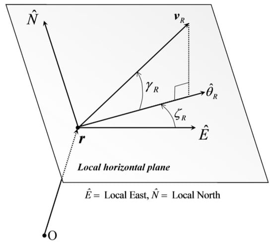The instantaneous position r is identified by three variables, i.e., (a) radius r $\left(=\left|\mathbf{r}\right|\right)$, (b) geographical longitude ${\lambda }_g$, and (c) latitude $\phi$. The relative velocity ${\mathbf{v}}_R$ is associated with (a) its magnitude $v_R$, (b) the relative flight path angle ${\gamma }_R$, and (c) the relative heading angle ${\zeta }_R$. The latter quantities identify the direction of ${\mathbf{v}}_R$ in the local horizontal plane, which is orthogonal to r and contains the local East and North unit vectors, denoted with $\widehat{E}\mathrm{and}\widehat{N}$ in Figure 1

Figure 1. Relative velocity and related angles in the local horizontal frame.

The kinematics equations govern the time evolution of r, ${\lambda }_g$, and $\phi$ [26,27],

$$\dot{r}=v_R\sin {\gamma }_R\hspace{1em}{\dot{\lambda }}_g={\displaystyle \frac{v_R\cos {\gamma }_R\cos {\zeta }_R}{r\cos \phi }}\hspace{1em}\dot{\phi }={\displaystyle \frac{v_R\cos {\gamma }_R\sin {\zeta }_R}{r}}$$

(48)

The aerospace vehicle is subject both to external actions (i.e., the gravitational force G and the aerodynamics force A) and to propulsive thrust T. Due to the relatively short time of flight, only the main harmonic of geopotential is considered, and the gravitational acceleration obeys the inverse square law as a result. Moreover, in general, the aerodynamic interaction includes three terms, i.e., (i) lift L, (ii) drag D, and (iii) side force Q. However, usually the latter is modest if compared to lift and drag; thus, it is neglected hence forward. The magnitudes of the aerodynamics accelerations, $\left(L/\tilde{m}\right)$ and $\left(D/\tilde{m}\right)$, depend on $v_R$ and r,

$${\displaystyle \frac{L}{\tilde{m}}}={\displaystyle \frac{1}{2}}{c}_L\left(M,\alpha \right){\displaystyle \frac{S}{\tilde{m}}}{\rho }_A\left(r\right)v_R^2\mathrm{and}{\displaystyle \frac{D}{\tilde{m}}}={\displaystyle \frac{1}{2}}{c}_D\left(M,\alpha \right){\displaystyle \frac{S}{\tilde{m}}}{\rho }_A\left(r\right)v_R^2$$

(49)

where $c_L$ and $c_D$ are respectively the dimensionless lift and drag coefficients, which depend on the Mach number M and the angle of attack $\alpha$ [26,27], whereas S is the aerodynamic surface and ${\rho }_A$ denotes the atmospheric density, which is a function of the instantaneous radius r. Let $\mu$ denote the gravitational parameter of the planet. The dynamics equations of atmospheric flight are written under the assumption that the thrust is always aligned with the rocket longitudinal axis, and are given by

$$\begin{array}{l}{\dot{\gamma }}_R=\left(-{\displaystyle \frac{\mu }{r^2{v}_R}}+{\displaystyle \frac{v_R}{r}}\right)\cos {\gamma }_R+{\displaystyle \frac{1}{v_R}}\left({\displaystyle \frac{L}{\tilde{m}}}+{\displaystyle \frac{T}{\tilde{m}}}\sin \alpha \right)\cos \sigma +2{\omega }_E\cos \phi \cos {\zeta }_R\\ +{\displaystyle \frac{{\omega }_E^{2}r}{v_R}}\cos \phi \left(\cos \phi \cos {\gamma }_R+\sin \phi \sin {\gamma }_R\sin {\zeta }_R\right)\end{array}$$

(50)

$${\dot{v}}_R=-{\displaystyle \frac{\mu }{r^2}}\sin {\gamma }_R-{\displaystyle \frac{D}{\tilde{m}}}+{\displaystyle \frac{T}{\tilde{m}}}\cos \alpha +{\omega }_E^{2}r\cos \phi \left(\cos \phi \sin {\gamma }_R-\sin \phi \cos {\gamma }_R\sin {\zeta }_R\right)$$

(51)

$$\begin{array}{l}{\dot{\zeta }}_R=-{\displaystyle \frac{v_R}{r}}\tan \phi \cos {\gamma }_R\cos {\zeta }_R-{\displaystyle \frac{\sin \sigma }{v_R\cos {\gamma }_R}}\left({\displaystyle \frac{L}{\tilde{m}}}+{\displaystyle \frac{T}{\tilde{m}}}\sin \alpha \right)+2{\omega }_E\cos \phi \tan {\gamma }_R\sin {\zeta }_R\\ \hspace{1em} -{\displaystyle \frac{{\omega }_E^{2}r}{v_R\cos {\gamma }_R}}\sin \phi \cos \phi \cos {\zeta }_R-2{\omega }_E\sin \phi \end{array}$$

(52)

where $\sigma$ denotes the bank angle, $\left(L/\tilde{m}\right)$, $\left(D/\tilde{m}\right)$, and $\tilde{m}$ are given by Equations (47) and (49), and $T=T_k^{\left(max\right)}$. Angle $\sigma$, together with the angle of attack, identifies the thrust direction needed to properly steer the launch vehicle during ascent. In short, the state and control vectors, x and u, are given by $x={\left[\begin{array}{cccccc}r& {\lambda }_g& \phi & {\gamma }_R& v_R& {\zeta }_R\end{array}\right]}^T$ and $u={\left[\begin{array}{cc}\alpha & \sigma \end{array}\right]}^T$.

Exoatmospheric flight is also conveniently described in spherical coordinates, making reference to the vehicle position and inertial velocity vectors, r and v. The instantaneous position r is identified by three variables, i.e., (a) radius r $\left(=\left|\mathbf{r}\right|\right)$, (b) absolute longitude ${\lambda }_a$, and (c) latitude $\phi$. Velocity v is associated with (a) its magnitude $v$, (b) the flight path angle $\gamma$, and (c) the heading angle $\zeta$. The latter quantities identify the direction of v in the local horizontal plane, in the same way as the direction of ${\mathbf{v}}_R$ is identified by ${\gamma }_R$ and ${\zeta }_R$ (cf. Figure 1). In spaceflight, the thrust direction can be expressed through two angles, ${\alpha }_T$ and ${\beta }_T$, and the equations of motion are

$$\dot{r}=v\sin \gamma \hspace{1em}{\dot{\lambda }}_a={\displaystyle \frac{v\cos \gamma \cos \zeta }{r\cos \phi }}\hspace{1em}\dot{\phi }={\displaystyle \frac{v\cos \gamma \sin \zeta }{r}}$$

(53)

$$\dot{\gamma }=\left(-{\displaystyle \frac{\mu }{r^{2}v}}+{\displaystyle \frac{v}{r}}\right)\cos \gamma +{\displaystyle \frac{T}{\tilde{m}v}}\cos {\beta }_T\sin {\alpha }_T$$

(54)

$$\dot{v}=-{\displaystyle \frac{\mu }{r^2}}\sin \gamma +{\displaystyle \frac{T}{\tilde{m}}}\cos {\alpha }_T\cos {\beta }_T$$

(55)

$$\dot{\zeta }=-{\displaystyle \frac{v}{r}}\tan \phi \cos \gamma \cos \zeta +{\displaystyle \frac{T}{\tilde{m}}}{\displaystyle \frac{\sin {\beta }_T}{v\cos \gamma }}$$

(56)

In short, the state and control vectors, x and u, are given by $x={\left[\begin{array}{cccccc}r& {\lambda }_a& \phi & \gamma & v& \zeta \end{array}\right]}^T$ and $u={\left[\begin{array}{cc}{\alpha }_T& {\beta }_T\end{array}\right]}^T$.

These two distinct sets of state and control variables are useful in different arcs. In fact, the governing Equations (48) and (50)–(52) and the respective state and control vectors can be employed for arcs 1 and 2, while Equations (53)–(56) and the respective state and control vectors are conveniently used in arcs 3 and 4, which precede orbit injection.

4.2. Formulation of the Problem

At time $t_0$, which is specified and is set to 0 without any loss of generality, the launch vehicle ends its initial vertical path, immediately after liftoff, and arc 1 begins. The initial conditions are all specified, i.e.,

$$x_0-x_{sp}=\mathbf{0}$$

(57)

where subscript sp denotes a specified value. The final orbit is assumed to have prescribed semimajor axis $a_{sp}$, eccentricity $e_{sp}$, and inclination $i_{sp}$. The desired right ascension of the ascending node can be achieved by choosing the initial Greenwich sidereal time at $t_0$, as shown in Ref. [28]

At time $t_1$, the first stage is released, and the second stage is ignited. If $t_{BO1}$ denotes the burnout time of stage 1 (starting from time $t_0$), then

$${\psi }_1=t_1-t_{BO1}$$

(58)

Moreover, all the state variables are continuous across $t_1$, and this means that the matching relation (3) is

$${\chi }_1=x_{ini}^{\left(2\right)}-x_{fin}^{\left(1\right)}$$

(59)

At time $t_2$, the second stage is released, and subrocket 3 starts traveling a ballistic (unpowered) arc. If $t_{BO2}$ denotes the burnout time of stage 2, then

$${\psi }_2=t_2-\left(t_{BO1}+t_{BO2}\right)$$

(60)

Two different sets of state and control variables are used in arcs 2 and 3, therefore matching relations must be identified that relate $\left(r,{\lambda }_g,\phi ,{\gamma }_R,v_R,{\zeta }_R\right)$ to $\left(r,{\lambda }_a,\phi ,\gamma ,v,\zeta \right)$. First, both radius and latitude have the same definition in arcs 2 and 3, and this means that

$$x_{1,ini}^{\left(3\right)}-x_{1,fin}^{\left(2\right)}=0\mathrm{and}{x}_{3,ini}^{\left(3\right)}-x_{3,fin}^{\left(2\right)}=0$$

(61)

The geographical and absolute longitude are related through the Greenwich sidereal time at $t_2$,

$$x_{2,ini}^{\left(3\right)}-\left[x_{2,fin}^{\left(2\right)}+{\theta }_{G0}+{\omega }_E\left(t_{BO1}+t_{BO2}\right)\right]=0$$

(62)

where ${\omega }_E$ denotes the Earth rotation rate, while ${\theta }_{G0}$ represents the Greenwich sidereal time at $t_0$. To obtain the remaining relations involving $\left({\gamma }_R,v_R,{\zeta }_R\right)$ and $\left(\gamma ,v,\zeta \right)$, the definition of ${\mathbf{v}}_R$ is projected onto the local horizontal plane, to yield

$$x_{5,ini}^{\left(3\right)}\sin x_{4,ini}^{\left(3\right)}-x_{5,fin}^{\left(2\right)}\sin x_{4,fin}^{\left(2\right)}=0$$

(63)

$$x_{5,ini}^{\left(3\right)}\cos x_{4,ini}^{\left(3\right)}\cos x_{6,ini}^{\left(3\right)}-x_{5,fin}^{\left(2\right)}\cos x_{4,fin}^{\left(2\right)}\cos x_{6,fin}^{\left(2\right)}-{\omega }_E{x}_{1,fin}^{\left(2\right)}\cos x_{3,fin}^{\left(2\right)}=0$$

(64)

$$x_{5,ini}^{\left(3\right)}\cos x_{4,ini}^{\left(3\right)}\sin x_{6,ini}^{\left(3\right)}-x_{5,fin}^{\left(2\right)}\cos x_{4,fin}^{\left(2\right)}\sin x_{6,fin}^{\left(2\right)}=0$$

(65)

where $x_{1,fin}^{\left(2\right)}=r\left(t_2\right)$, $x_{3,fin}^{\left(2\right)}=\phi \left(t_2\right)$, $x_{4,fin}^{\left(2\right)}={\gamma }_R\left(t_2\right)$, $x_{4,ini}^{\left(3\right)}=\gamma \left(t_2\right)$, $x_{5,fin}^{\left(2\right)}=v_R\left(t_2\right)$, $x_{5,ini}^{\left(3\right)}=v\left(t_2\right)$, $x_{6,fin}^{\left(2\right)}={\zeta }_R\left(t_2\right)$, and $x_{6,ini}^{\left(3\right)}=\zeta \left(t_2\right)$. The preceding relations (61)–(65) are written as implicit state transformation, in the form ${\chi }_2\left(x_{ini}^{\left(3\right)},x_{fin}^{\left(2\right)}\right)=\mathbf{0}$. This mapping establishes a bijective relation between the two state representations, in the open set defined by the following inequalities: (a) $r>0$, (b) $\phi \ne \pm \pi /2$, (c) $v_R>0$, (d) $v>0$. Inequality (a) means that the launch vehicle does not reach the center of the main attracting body, (b) implies that the rocket must not fly over the North Pole or South Pole, whereas (c) and (d) mean that the magnitude of both the relative and the inertial velocity must not vanish. It is apparent that the open set at hand, in which the governing Equations (48) and (50)–(56) are nonsingular, virtually includes all the ascent paths of practical interest.

At time $t_3$, the third stage is ignited. All the state variables are continuous across $t_3$, and this means that the matching relation (3) is

$${\chi }_3=x_{ini}^{\left(4\right)}-x_{fin}^{\left(3\right)}$$

(66)

Because $t_3$ is unspecified and no further condition holds at $t_3$, ${\psi }_3$ is identically zero (cf. Section 2).

At time $t_f$, the upper stage must reach proper final conditions that correspond to insertion into the desired orbit. The vis viva equation for energy [25] leads to obtaining the semimajor axis a in terms of final position and velocity,

$$a_{sp}={\displaystyle \frac{\mu x_{1,f}}{2\mu -x_{1,f}{x}_{5,f}^2}}\Rightarrow a_{sp}{x}_{5,f}^2{x}_{1,f}+\mu x_{1,f}-2\mu a_{sp}=0$$

(67)

Moreover, the relation on the specific angular momentum [25], combined with Equation (67), provides the second final condition,

$${\mu }^2{x}_{1,f}\left(1-e_{sp}^2\right)-\left(2\mu -x_{1,f}{x}_{5,f}^2\right){\left(x_{1,f}{x}_{5,f}\cos x_{4,f}\right)}^2=0$$

(68)

Finally, the orbit inclination is directly related to the latitude and heading angle; therefore, the following relation must hold [25]:

$$\cos x_{3,f}\cos x_{6,f}-\cos i_{sp}=0$$

(69)

Equations (57) and (67)–(69) are all incorporated as components of $\zeta$ (cf. Equation (2)).

The optimal ascent path of the multistage launch vehicle minimizes propellant consumption of the upper stage, through selection of time $t_3$ and of the thrust direction time history, associated with either angles $\left(\alpha ,\sigma \right)$ (in arcs 1 and 2) or angles $\left({\alpha }_T,{\beta }_T\right)$ (in arcs 3 and 4). Because stage 3 employs maximum thrust during its powered phase (i.e., arc 4), minimizing propellant consumption is equivalent to minimizing the ignition time. This circumstance implies that the objective function to minimize is

$$J\equiv \varphi =t_f-t_3$$

(70)

4.3. Necessary Conditions

The minimum-fuel ascent path obeys the governing (state) equations in their respective arcs (cf. Section 4.1) and must satisfy

(a)

the boundary conditions at $t_0$ and $t_f$, collected in vector $\zeta$ (cf. Equation (2)),

(b)

the junction conditions (58)–(66), and

(c)

the necessary conditions (14)–(16) and (19)–(22) (while Equation (18) is unnecessary for the case at hand, because no parameter vector p is introduced).

This subsection only focuses on the multipoint conditions (19)–(21), for the purpose of showing that they can be solved sequentially. At all intermediate times $t_1$, $t_2$, $t_3$, ${\psi }_j$ is independent of $x_{ini}^{\left(j+1\right)}\mathrm{and}{x}_{fin}^{\left(j\right)}$, thus the multipoint conditions are of class C. Moreover, because $\varphi$ is independent of $x_{ini}^{\left(j+1\right)}\mathrm{and}{x}_{fin}^{\left(j\right)}$ as well, the implicit costate transformation (45) reduces to

$${\lambda }_{ini}^{\left(j+1\right)}=-{\left({\displaystyle \frac{\partial {\chi }_j}{\partial x_{ini}^{\left(j+1\right)}}}\right)}^T{\left({\displaystyle \frac{\partial {\chi }_j}{\partial x_{fin}^{\left(j\right)}}}\right)}^{-T}{\lambda }_{fin}^{\left(j\right)}.$$

(71)

More specifically, at time $t_1$, Equation (59), combined with Equation (71), leads to ${\lambda }_{ini}^{\left(2\right)}={\lambda }_{fin}^{\left(1\right)}$, i.e., the costate is continuous across $t_1$. The remaining unknowns, i.e., ${\upsilon }_1$ and ${\xi }_1$, can be found using Equation (43) for ${\upsilon }_1$, followed by Equation (19) for ${\xi }_1$ Because of Equation (58), at $t_1$ Equation (19) yields

$${\xi }_1=H_{ini}^{\left(2\right)}-H_{fin}^{\left(1\right)}.$$

(72)

At time $t_2$, Equation (71) provides the jump relation for the costate, which is not continuous because of the form of ${\chi }_2\left(x_{ini}^{\left(3\right)},x_{fin}^{\left(2\right)}\right)$, which incorporates Equations (61)–(65). The remaining unknown, i.e., ${\upsilon }_3$ can be found using Equation (43) for ${\upsilon }_2$, followed by Equation (19) for ${\xi }_2$. Because of Equation (60), at $t_2$, Equation (19) yields

$${\xi }_2=H_{ini}^{\left(3\right)}-H_{fin}^{\left(2\right)}.$$

(73)

At time $t_3$, Equation (66), combined with Equation (71) leads to ${\lambda }_{ini}^{\left(4\right)}={\lambda }_{fin}^{\left(3\right)}$, i.e., the costate is continuous across $t_3$. The remaining unknown, i.e., ${\upsilon }_3$ can be found using Equation (43), whereas ${\xi }_3$ is irrelevant because ${\psi }_3=0$. Because of Equation (70), at $t_3$, Equation (19) yields

$$H_{ini}^{\left(4\right)}-H_{fin}^{\left(3\right)}=-1$$

(74)

The preceding steps show that the multipoint corner conditions can be solved sequentially for the problem at hand, while the remaining necessary conditions coincide with those associated with single-arc optimal control problems.

5. Application 2: Low-Thrust Orbit Transfer with Eclipsing

This section focuses on low-thrust orbit transfers about a single attracting body, under the assumption that the latter has spherical mass distribution. This implies that the gravitational acceleration obeys the inverse square law. If compared to chemical propulsion, low-thrust systems allow for considerable reduction in the propellant mass needed to complete orbit transfers, at the price of considerably increasing the time of flight. Moreover, low-thrust technology relies on the availability of electrical power to operate. Consequently, low-thrust systems are switched off along eclipse arcs, in which the celestial body of interest shadows the spacecraft. Because low-thrust transfers are usually very long, minimum-time solutions are sought, under the assumption that thrusting is available only in illuminated (light) arcs. The underlying trajectory optimization problem is very challenging, because the control authority (i.e., thrusting) is state-dependent.

Extensive literature exists on low-thrust orbit transfers with eclipsing, using regularization or averaging [29,30,31,32,33]. Recently, the author formulated the problem at hand as a multi-arc trajectory optimization problem [21], composed of an unspecified number of thrust and coast arcs, separated by light-shadow transitions. In this section, the general approach presented in Section 2 and Section 3 is applied to formulating a low-thrust Earth orbit transfer with eclipse constraints, for the purpose of demonstrating that the multipoint corner conditions are solvable sequentially.

Based on the analysis—relying on the Pontryagin minimum principle—contained in previous work [21], thrust is maximum along light arcs, while it is switched off along eclipse arcs, as already remarked. This allows for writing the thrust acceleration in arc k as a function of time, under the assumption that the effective exhaust velocity is constant,

$${\displaystyle \frac{T_k}{{\tilde{m}}_k}}={\displaystyle \frac{T_k{c}^{\left(ex\right)}}{c^{\left(ex\right)}{\tilde{m}}_{k,ini}-T_k\left(t-t_{k-1}\right)}}$$

(75)

where symbols $T_k$ and ${\tilde{m}}_k$ denote thrust and mass, with $T_k=T^{\left(max\right)}$ (in light arcs) or $T_k=0$ (in eclipse arcs), whereas $c^{\left(ex\right)}$ is the (constant) effective exhaust velocity of the propulsion system and t represents the actual time.

5.1. State Representations

The spacecraft is modeled as a point mass, and its state is identified through two distinct representations, i.e., (a) spherical coordinates and (b) modified equinoctial elements (MEE). The use of the latter variables is related to two favorable circumstances [21]: (i) using MEE, 9 out of 14 components of state and costate are constant along coast arcs, and (ii) the initial values of the adjoint variables associated with MEE exhibit reduced sensitivity with respect to the corresponding variables associated with spherical coordinates [21,34,35]. However, the latter remain very useful in the derivation of closed-form jump relations at light–shadow transitions.

Spherical coordinates are closely related to the spacecraft position r and velocity v. Three variables identify position, i.e., (a) radius r $\left(=\left|\mathbf{r}\right|\right)$, (b) absolute longitude ${\lambda }_a$, and (c) latitude $\phi$. Velocity is conveniently described in terms of its radial, East, and North components (in the local horizontal plane), denoted with $v_r$, $v_E$, and $v_N$, respectively. The preceding six variables are collected in $y={\left[\begin{array}{cccccc}{y}_1& y_2& y_3& y_4& y_5& y_6\end{array}\right]}^T={\left[\begin{array}{cccccc}r& {\lambda }_a& \phi & v_r& v_E& v_N\end{array}\right]}^T$. The related state equations are reported in Ref. [23] and omitted in this work, for the sake of conciseness. They also involve two control variables, i.e., the thrust angles, which identify the instantaneous thrust direction in the local horizontal frame (cf. Figure 1).

Low-thrust transfers can also be described using osculating orbit elements, i.e., semimajor axis a, eccentricity e, inclination i, right ascension of the ascending node $\Omega$, argument of perigee $\omega$, and true anomaly f [25]. However, because some orbit elements are not defined for circular or equatorial orbit (and also when an elliptic orbit transitions to a hyperbola), MEE were introduced [36,37] and are defined as

$$\begin{array}{lll}{z}_1=a\left(1-e^2\right)& z_2=e\cos \left(\Omega +\omega \right)& z_3=e\sin \left(\Omega +\omega \right)\\ z_4=\tan {\displaystyle \frac{i}{2}}\cos \Omega & z_5=\tan {\displaystyle \frac{i}{2}}\sin \Omega & z_6=\Omega +\omega +f\end{array}.$$

(76)

These components form the state vector z. Their governing equations [26,36] are omitted for the sake of brevity. They also involve two control variables, i.e., the two thrust angles $\left(u_1,u_2\right)$ in the local vertical local horizontal (LVLH) frame. This reference system is associated with the right-hand sequence of unit vectors $\left(\widehat{r},\widehat{\theta },\widehat{h}\right)$, with $\widehat{r}$ aligned with the spacecraft position (taken from the center of mass of the attracting body) and $\widehat{h}$ pointing toward the angular momentum.

MEE and spherical coordinates are related through the following six relations [23], which define the left-hand sides of the implicit state transformation $\eta \left(y,z\right)=0$

$$\begin{array}{ll}{\eta }_1& =z_1\left[\left(z_4^2-z_5^2+1\right)\cos z_6+2z_4{z}_5\sin z_6\right]\\ & -\left(1+z_2\cos z_6+z_3\sin z_6\right)\left(z_4^2+z_5^2+1\right)y_1\cos y_2\cos y_3\end{array}$$

(77)

$$\begin{array}{ll}{\eta }_2& =z_1\left[\left(z_4^2-z_5^2+1\right)\sin z_6+2z_4{z}_5\cos z_6\right]\\ & -\left(1+z_2\cos z_6+z_3\sin z_6\right)\left(z_4^2+z_5^2+1\right)y_1\sin y_2\cos y_3\end{array}$$

(78)

$${\eta }_3=2z_1\left(z_4\sin z_6-z_5\cos z_6\right)-\left(1+z_2\cos z_6+z_3\sin z_6\right)\left(z_4^2+z_5^2+1\right)y_1\sin y_3$$

(79)

$$\begin{array}{ll}{\eta }_4& =-\sqrt{\mu }\left[\left(z_3+\sin z_6\right)\left(1+z_4^2-z_5^2\right)-2z_4{z}_5\left(z_2+\cos z_6\right)\right]\\ & -\sqrt{z_1}\left(z_4^2+z_5^2+1\right)\left(y_4\cos y_3\cos y_2-y_5\sin y_2-y_6\sin y_3\cos y_2\right)\end{array}$$

(80)

$$\begin{array}{ll}{\eta }_5& =-\sqrt{\mu }\left[\left(z_3+\cos z_6\right)\left(1+z_5^2-z_4^2\right)-2z_4{z}_5\left(z_3+\sin z_6\right)\right]\\ & -\sqrt{z_1}\left(z_4^2+z_5^2+1\right)\left(y_4\cos y_3\sin y_2+y_5\cos y_2-y_6\sin y_3\sin y_2\right)\end{array}$$

(81)

$${\eta }_6=2\sqrt{\mu }\left(z_4\cos z_6+z_5\sin z_6+z_2{z}_4+z_3{z}_5\right)-\sqrt{z_1}\left(z_4^2+z_5^2+1\right)\left(y_4\sin y_3+y_6\cos y_3\right).$$

(82)

The transformation at hand is defined over the open subset identified by the following inequalities:

$$z_1>0,\hspace{1em}{z}_2\cos x_6+z_3\sin z_6+1>0,\hspace{1em}{y}_1>0,\hspace{1em}-{\displaystyle \frac{\pi }{2}}<y_3<{\displaystyle \frac{\pi }{2}}$$

(83)

The first inequality rules out rectilinear trajectories, the second one corresponds to finite distance from the attracting body [26], $y_1>0$ implies that the spacecraft does not reach the center of the attracting body, and the last inequality is related to the definition of latitude (and implies that the spacecraft does not travel over the poles). It is apparent that Equation (83) defines two open sets (for z and y), which virtually include all the space trajectories of practical interest. The implicit state transformation at hand represents an isomorphic mapping between spherical coordinates and MEE in the open set defined by Equation (83). The Jacobian matrices $\partial \eta /\partial y$ and $\partial \eta /\partial z$ are straightforward to obtain from Equations (77)–(82) and are nonsingular, due to the isomorphic (bijective) nature of the state transformation in the open sets identified by Equation (83).

5.2. Spacecraft Eclipsing

The main attracting body, i.e., Earth hence forward, shadows the spacecraft multiple times during the orbit transfer. The eclipse condition can be derived in terms of either spherical coordinates or MEE, under two very reasonable simplifying assumptions: (i) the Earth describes a circular orbit about the Sun, and (ii) the shadow is cylindrical. Assumption (i) represents a very good approximation because of the modest eccentricity of the Earth orbit. Approximation (ii) is very frequently used due to the large distance that separates Earth and the Sun. In this subsection, several analytical developments are omitted for the sake of brevity and can be found in Ref. [23].

Using spherical coordinates, the spacecraft is eclipsed if

$$y_1\cos y_3\cos y_2\cos {\theta }_S+y_1\cos y_3\sin y_2\sin {\theta }_S\cos \epsilon +y_1\sin y_3\sin {\theta }_S\sin \epsilon +\sqrt{y_1^2-R_E^2}\le 0$$

(84)

where $R_E$ is the Earth radius, $\epsilon$ is the ecliptic obliquity, whereas ${\theta }_S$ is the ecliptic longitude, which identifies the instantaneous position of the Sun. If ${\theta }_{S0}$ denotes the value of ${\theta }_S$ at the initial time $t_0$ (set to 0) and ${\omega }_S\left(=2\pi /T_S;T_S=1\mathrm{year}\right)$ is the (constant) angular rate of the Sun in its motion relative to Earth, then ${\theta }_S={\omega }_{S}t+{\theta }_{S0}$. The lleft-hand side of Equation (84) is incorporated into the e equality $S_y\left(y_1,y_2,y_3,{\theta }_S\right)=0$, which identifies light–shadow transitions.

Using MEE, the spacecraft is eclipsed if

$$\begin{array}{l}{z}_1\left\{\left[\left(z_4^2-z_5^2+1\right){\mathrm{c}}_{z_6}+2z_4{z}_5{s}_{z_6}\right]{\mathrm{c}}_{{\theta }_S}+\left[\left(z_5^2-z_4^2+1\right)s_{z_6}+2z_4{z}_5{\mathrm{c}}_{z_6}\right]{\mathrm{s}}_{{\theta }_S}{\mathrm{c}}_{\epsilon }+2\left(z_4{s}_{z_6}-z_5{\mathrm{c}}_{z_6}\right){\mathrm{s}}_{{\theta }_S}{\mathrm{s}}_{\epsilon }\right\}\\ +\left(z_4^2+z_5^2+1\right)\sqrt{z_1^2-R_E^2{\left(1+z_2{\mathrm{c}}_{z_6}+z_3{\mathrm{s}}_{z_6}\right)}^2}\le 0\end{array}$$

(85)

where ${\mathrm{c}}_{\vartheta }:=\cos \vartheta$ and $s_{\vartheta }:=\sin \vartheta$ ($\vartheta$ denotes a generic angle). The left-hand side of Equation (85) is incorporated into the equality $S_z\left(z_1,z_2,z_3,z_4,z_5,z_6,{\theta }_S\right)=0$, which identifies light/shadow transitions. It is worth noting that $S_z$ depends on all the components of z, unlike $S_y$, which is a function of only 3 components of y.

5.3. Formulation of the Problem

The initial and final orbits are identified through the specified values of some MEE. In transfer problems, the true anomaly is not prescribed at the initial and final time, whereas the remaining elements can be either specified or not. Regardless of the specific case, the boundary conditions are expressed in the form of Equation (2), where x coincides with z.

Because thrust is available only when the spacecraft is illuminated, the entire transfer path is composed of an unspecified number of light and eclipse arcs. The problem is formulated as a multi-arc trajectory optimization problem, with the thrust acceleration magnitude given by Equation (75). In arc k, thrust is conveniently projected onto the LVLH-frame, through angles $\left(u_1,u_2\right)$, which form the control vector u $\left(={\left[\begin{array}{cc}{u}_1& u_2\end{array}\right]}^T\right)$,

$$a_{r,k}={\displaystyle \frac{T_k}{{\tilde{m}}_k}}\cos u_{2,k}\sin u_{1,k}\hspace{1em}{a}_{\theta ,k}={\displaystyle \frac{T_k}{{\tilde{m}}_k}}\cos u_{2,k}\cos u_{1,k}\hspace{1em}{a}_{h,k}={\displaystyle \frac{T_k}{{\tilde{m}}_k}}\sin u_{2,k}$$

(86)

Light–shadow transitions correspond to vanishing of the left-hand side of Equation (85). However, in the following, the use of Equation (84) in place of Equation (85) will be shown to be advantageous.

The minimum-time orbit transfer is sought, through selection of the unknown values of MEE of the initial and final orbit and the identification of the optimal thrust direction time history. Hence, the objective function to minimize is

$$J\equiv \varphi =t_f$$

(87)

5.4. Necessary Conditions

The minimum-time transfer path obeys the governing (state) equations in their respective arcs and must satisfy

(a)

the boundary conditions at $t_0$ and $t_f$, collected in vector $\zeta$(cf. Equation (2)),

(b)

the junction conditions (58)–(66), and

(c)

the necessary conditions (14)–(16) and (19)–(22) (while Equation (18) is unnecessary for the case at hand, because no parameter vector p is introduced).

As a preliminary step, the minimum principle (22) is applied, with reference to both state representations, associated with y (spherical coordinates) and z (MEE). The respective adjoint variables are denoted with ${\lambda }_y$ and ${\lambda }_z$, respectively. Then, the expressions of the control variables written in terms of state (y or z) and costate (${\lambda }_y$ or ${\lambda }_z$) are inserted into the Hamiltonian function, thus identifying the partitions of ${\lambda }_y$ and ${\lambda }_z$, i.e., ${\lambda }_y={\left[\begin{array}{cc}{\lambda }_{y,L}^T& {\lambda }_{y,NL}^T\end{array}\right]}^T$ and ${\lambda }_z={\left[\begin{array}{cc}{\lambda }_{z,L}^T& {\lambda }_{z,NL}^T\end{array}\right]}^T$.

If spherical coordinates are employed, then the Hamiltonian function assumes the form [23]

$$H_y^{\left(k\right)}=H_{y,0}^{\left(k\right)}-{\displaystyle \frac{T_k}{{\tilde{m}}_k}}\sqrt{{\left({\lambda }_{y,4}^{\left(k\right)}\right)}^2+{\left({\lambda }_{y,5}^{\left(k\right)}\right)}^2+{\left({\lambda }_{y,6}^{\left(k\right)}\right)}^2},t_{k-1}\le t\le t_k$$

(88)

where ${\lambda }_{y,i}^{\left(k\right)}$ represents component i of the adjoint vector ${\lambda }_y^{\left(k\right)}$, whereas symbol $H_{y,0}^{\left(k\right)}$ denotes a function independent of ${\lambda }_y^{\left(k\right)}$. Therefore, it is apparent that

$${\lambda }_{y,NL}={\left[\begin{array}{ccc}{\lambda }_{y,4}& {\lambda }_{y,5}& {\lambda }_{y,6}\end{array}\right]}^T\mathrm{and}{y}_{NL}={\left[\begin{array}{ccc}{y}_4& y_5& y_6\end{array}\right]}^T$$

(89)

Moreover, Equation (88) can be evaluated at $t_{k-1}\equiv t_j\left(k=2,\dots ,N\right)$, letting $y=x_{ini}^{\left(k\right)}\equiv x_{ini}^{\left(j+1\right)}$ and ${\lambda }_y={\lambda }_{ini}^{\left(k\right)}\equiv {\lambda }_{ini}^{\left(j+1\right)}$, and one recognizes

$$h_L=\mathbf{0}\mathrm{and}{h}_{NL}=H_{y,0}^{\left(k\right)}-{\displaystyle \frac{T_j}{{\tilde{m}}_j}}\sqrt{{\left({\lambda }_{4,ini}^{\left(j+1\right)}\right)}^2+{\left({\lambda }_{5,ini}^{\left(j+1\right)}\right)}^2+{\left({\lambda }_{6,ini}^{\left(j+1\right)}\right)}^2}$$

(90)

If MEE are used, then the Hamiltonian function assumes the form [23]

$$H_z^{\left(k\right)}=H_{z,0}^{\left(k\right)}-{\displaystyle \frac{T_k}{{\tilde{m}}_k}}\sqrt{{\left(H_{z,r}^{\left(k\right)}\right)}^2+{\left(H_{z,\theta }^{\left(k\right)}\right)}^2+{\left(H_{z,h}^{\left(k\right)}\right)}^2}$$

(91)

where $H_{z,0}^{\left(k\right)}$ denotes a function independent of ${\lambda }_z^{\left(k\right)}$, while $\left(H_{z,r}^{\left(k\right)},H_{z,\theta }^{\left(k\right)},H_{z,h}^{\left(k\right)}\right)$ represent three nonlinear functions in ${\lambda }_{z,1}$ through ${\lambda }_{z,6}$. Therefore, it is apparent that

$${\lambda }_{z,NL}\equiv {\lambda }_z\mathrm{and}{z}_{NL}\equiv z$$

(92)

Moreover, Equation (91) can be evaluated at $t_{k-1}\equiv t_j\left(k=2,\dots ,N\right)$, letting $z=x_{ini}^{\left(k\right)}\equiv x_{ini}^{\left(j+1\right)}$ and ${\lambda }_z={\lambda }_{ini}^{\left(k\right)}\equiv {\lambda }_{ini}^{\left(j+1\right)}$, and one recognizes

$$h_L=\mathbf{0}\mathrm{and}{h}_{NL}=H_{z,0}^{\left(k\right)}-{\displaystyle \frac{T_k}{{\tilde{m}}_k}}\sqrt{{\left(H_{z,r}^{\left(k\right)}\right)}^2+{\left(H_{z,\theta }^{\left(k\right)}\right)}^2+{\left(H_{z,h}^{\left(k\right)}\right)}^2}$$

(93)

This subsection is especially focused on the multipoint conditions (19)–(21), with the final aim of showing that they can be solved sequentially. This requires the combined use of spherical coordinates and MEE (cf. next subsection).

The shadow condition in terms of MEE (cf. Equation (85)) can be reduced to the form of Equation (4) by letting ${\psi }_j\left(x_{ini}^{\left(j+1\right)},t_j\right)={\left.S_z\left(z,{\theta }_S\left(t_j\right)\right)\right|}_{z=x_{ini}^{\left(j+1\right)}}$. Because ${\left(\partial {\psi }_j/\partial x_{ini}^{\left(j+1\right)}\right)}^T\ne \mathbf{0}$ and $\left(\partial {\psi }_j/\partial t_j\right)\ne 0$, the corner condition is of class A. However, from inspection of Equation (93), it is apparent that ${\left(\partial {\psi }_j/\partial x_{ini,NL}^{\left(j+1\right)}\right)}^T\ne \mathbf{0}$; therefore, the conditions of Proposition 2 do not hold, and the multipoint corner conditions are not amenable to a closed-form solution. This conclusion is also consistent with the analysis contained in Refs. [22,23].

The shadow condition in terms of spherical coordinates (cf. Equation (84)) can be reduced to the form of Equation (4) by letting ${\psi }_j\left(x_{ini}^{\left(j+1\right)},t_j\right)={\left.S_y\left(y,{\theta }_S\left(t_j\right)\right)\right|}_{y=x_{ini}^{\left(j+1\right)}}$ Because ${\left(\partial {\psi }_j/\partial x_{ini}^{\left(j+1\right)}\right)}^T\ne \mathbf{0}$ and $\left(\partial {\psi }_j/\partial t_j\right)\ne 0$, the corner condition is again of class A. Moreover, from the inspection of Equation (90), it is apparent that ${\left(\partial {\psi }_j/\partial x_{ini,NL}^{\left(j+1\right)}\right)}^T=\mathbf{0}$; therefore, the conditions of Proposition 2 hold, and the multipoint corner conditions are amenable to a closed-form solution, unlike what occurred with MEE.

5.5. Sequential Solution of the Multipoint Corner Conditions

Due to the latter favorable property of spherical coordinates, they can be employed for the purpose of deriving the closed-form jump relations of the costate at light–shadow transitions. This methodology was already successfully used [22,23] and requires a sequence of transformations at a light–shadow transition. Let $t_i^{\left(E\right)}\left(i=1,\dots ,N_E\right)$ denote a generic time at which light–shadow transitions occur. In the minimum-time problem at hand, $N_E$ is unknown a priori. However, in an iterative method, $N_E$ is guessed (and does not change in a given iteration) and the sequential solution of all corner conditions is leveraged. If all the boundary conditions (for both the state and the costate) are not met to a satisfying accuracy, then $N_E$ is adjusted and updated at the succeeding iteration.

With reference to a single iteration, the following steps allow obtaining closed-form jump relations at $t_i^{\left(E\right)}$ for the adjoint variables associated with the state equations.

Step 1. A light-shadow transition is detected at $t_i^{\left(E\right)}$, using MEE.

Step 2. Three subsequent times are defined in relation to $t_i^{\left(E\right)}$, i.e., (i) $t_j=t_i^{\left(E\right)}-{\epsilon }_1$, (ii) $t_{j+1}=t_i^{\left(E\right)}$, and (iii) $t_{j+2}=t_i^{\left(E\right)}+{\epsilon }_2$, where ${\epsilon }_1$ and ${\epsilon }_2$ denote two positive, arbitrarily small constants.

Step 3. At $t_j$, the initial costate along arc $\left(j+1\right)$, associated with spherical coordinates and denoted with ${\lambda }_{ini}^{\left(j+1\right)}={\lambda }_{y,ini}^{\left(j+1\right)}$, is obtained from the final costate associated with MEE in arc j, denoted with ${\lambda }_{fin}^{\left(j\right)}={\lambda }_{z,fin}^{\left(j\right)}$, by means of Proposition 3.

Step 4. At $t_{j+1}$, the initial costate along arc $\left(j+2\right)$, associated with spherical coordinates and denoted with ${\lambda }_{ini}^{\left(j+2\right)}={\lambda }_{y,ini}^{\left(j+2\right)}$, is obtained from the final costate associated with spherical coordinates in arc $\left(j+1\right)$, denoted with ${\lambda }_{fin}^{\left(j+1\right)}={\lambda }_{y,fin}^{\left(j+1\right)}$, through the use of Proposition 1.

Step 5. At $t_{j+2}$, the initial costate along arc $\left(j+3\right)$, associated with MEE and denoted with ${\lambda }_{ini}^{\left(j+3\right)}={\lambda }_{z,ini}^{\left(j+3\right)}$, is obtained from the final costate associated with spherical coordinates in arc $\left(j+2\right)$, denoted with ${\lambda }_{fin}^{\left(j+2\right)}={\lambda }_{y,fin}^{\left(j+2\right)}$, by means of Proposition 3.

In particular, Steps 3 and 5 employ the implicit costate transformation, which is a special case belonging to class C. In fact, at any arbitrary time (not necessarily associated with light–shadow transitions), the two state representations can be regarded as coexisting, and the respective costate vectors can be obtained using Equation (46). Moreover, because ${\epsilon }_1$ and ${\epsilon }_2$ are arbitrarily small, Steps 3 and 5 can be completed at $t_j$ and $t_{j+2}$ in the limit as ${\epsilon }_1\to 0^{+}$ and ${\epsilon }_2\to 0^{+}$. It is worth noticing that $\left(N_E-1\right)$ light-shadow transitions correspond to $3\left(N_E-1\right)$ times $t_j$.

The preceding steps show that the multipoint corner conditions can be solved sequentially for the problem at hand, while the remaining necessary conditions coincide with those associated with single-arc optimal control problems. In conclusion, thanks to the sequential (closed-form) solution of all the multipoint corner conditions, an indirect solution approach can manage the same unknown quantities associated with a single-arc optimal control problem. This remarkable fact is extremely useful in the numerical solution of minimum-time problems with an unknown number of arcs, such as that addressed in this section. For similar problems, alternative options exist, such as regularization [38], which does not use multiple arcs. While the two approaches are shown to yield near-identical numerical results [23], compared to regularization, the multi-arc formulation is shown to yield simpler adjoint equations and turns out to be unequivocally superior in terms of computational efficiency, thanks to the sequential solution of corner conditions.

5.6. Numerical Example: Low-Thrust Transfer from Geo-Transfer-Orbit to Geostationary Orbit

In Earth orbit transfers, the terminal (initial and final) orbits are defined by prescribing the values of some MEE, particularly those independent of the true anomaly, which instead is not specified. Specifically, this work considers a typical geo-transfer-orbit (GTO) as the initial orbit, associated with the following elements:

$$p_i=\mathrm{11,359}\mathrm{km}{e}_i=0.7306i_i=28.5\mathrm{deg}{\Omega }_i=0\mathrm{deg}{\omega }_i=0\mathrm{deg}$$

(94)

whereas the final orbit is geostationary, i.e.,

$$p_f=R_{geo}\hspace{1em}{e}_f=0\hspace{1em}{i}_f=0\hspace{1em}\left(R_{geo}=\mathrm{42,164}\mathrm{km}\right)$$

(95)

where subscripts i and f refer to the initial and final time. These boundary conditions can be rewritten in terms of MEE (cf. Equation (76)) as

$$\begin{array}{l}{x}_{1,0}-p_i=0\hspace{1em}{x}_{2,0}-e_i\cos \left({\Omega }_i+{\omega }_i\right)=0\hspace{1em}{x}_{3,0}-e_{i}sin\left({\Omega }_i+{\omega }_i\right)=0\\ x_{4,0}-\tan {\displaystyle \frac{i_i}{2}}\cos {\Omega }_i=0\hspace{1em}{x}_{5,0}-\tan {\displaystyle \frac{i_i}{2}}\sin {\Omega }_i=0\end{array}$$

(96)

$$x_{1,f}-R_{geo}=0\hspace{1em}{x}_{2,f}=0\hspace{1em}{x}_{3,f}=0\hspace{1em}{x}_{4,f}=0\hspace{1em}{x}_{5,f}=0$$

(97)

The left-hand sides of Equations (96) and (97) form vector $\zeta$ (cf. Equation (2)). Low-thrust propulsion is used, with initial thrust acceleration and effective exhaust velocity equal to $2.597\cdot {10}^{-4}\mathrm{m}/{\mathrm{s}}^2$ and $32.34\mathrm{km}/\mathrm{s}$, respectively. The reference epoch is 22 March 2000. The preceding boundary conditions, propulsion parameters, and epoch coincide with those reported in Ref. [39].

The numerical solution to this problem is obtained with the use of the indirect heuristic method [23], which assumes the initial values of the adjoint variables and the time of flight as the unknowns, before enforcing the analytical conditions for optimality. No additional unknown referring to intermediate times is introduced, and the sequential solution of corner conditions implies their fulfillment. Further details on this are provided in Ref. [23].

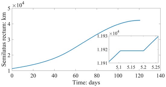
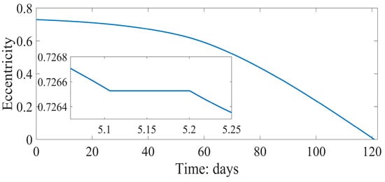
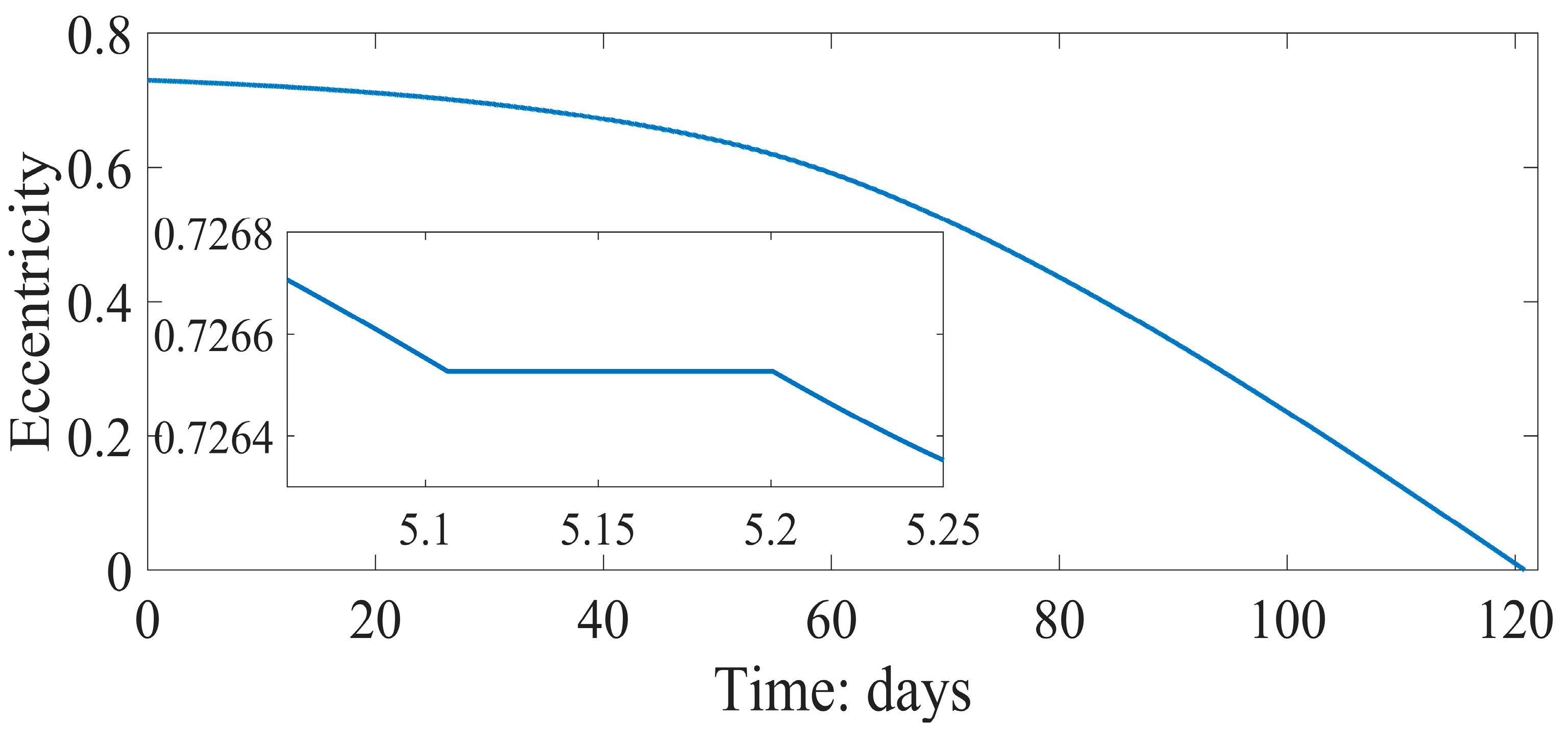
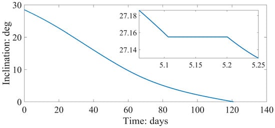
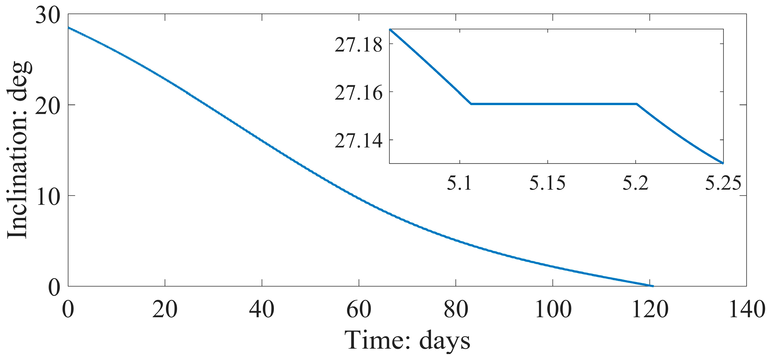
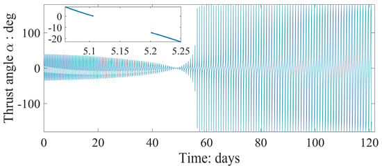
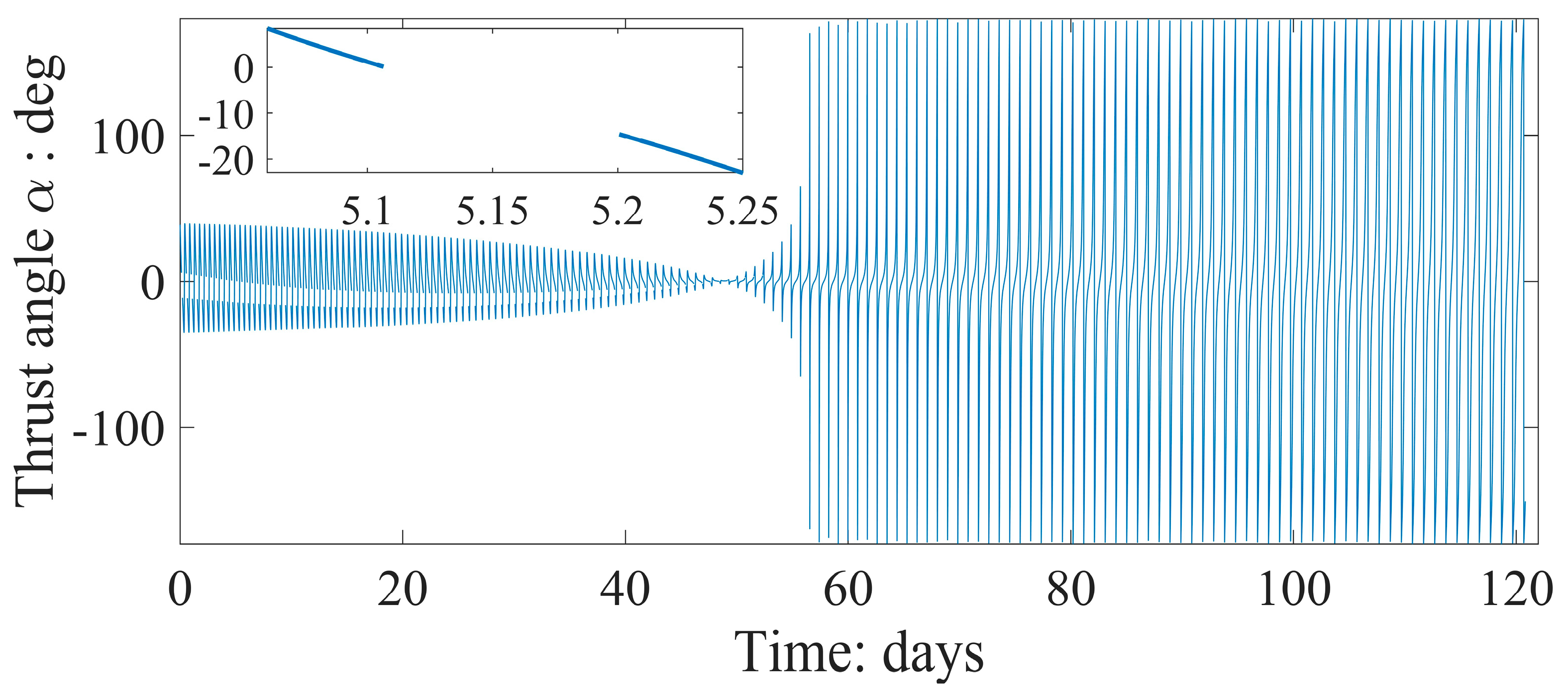
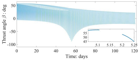
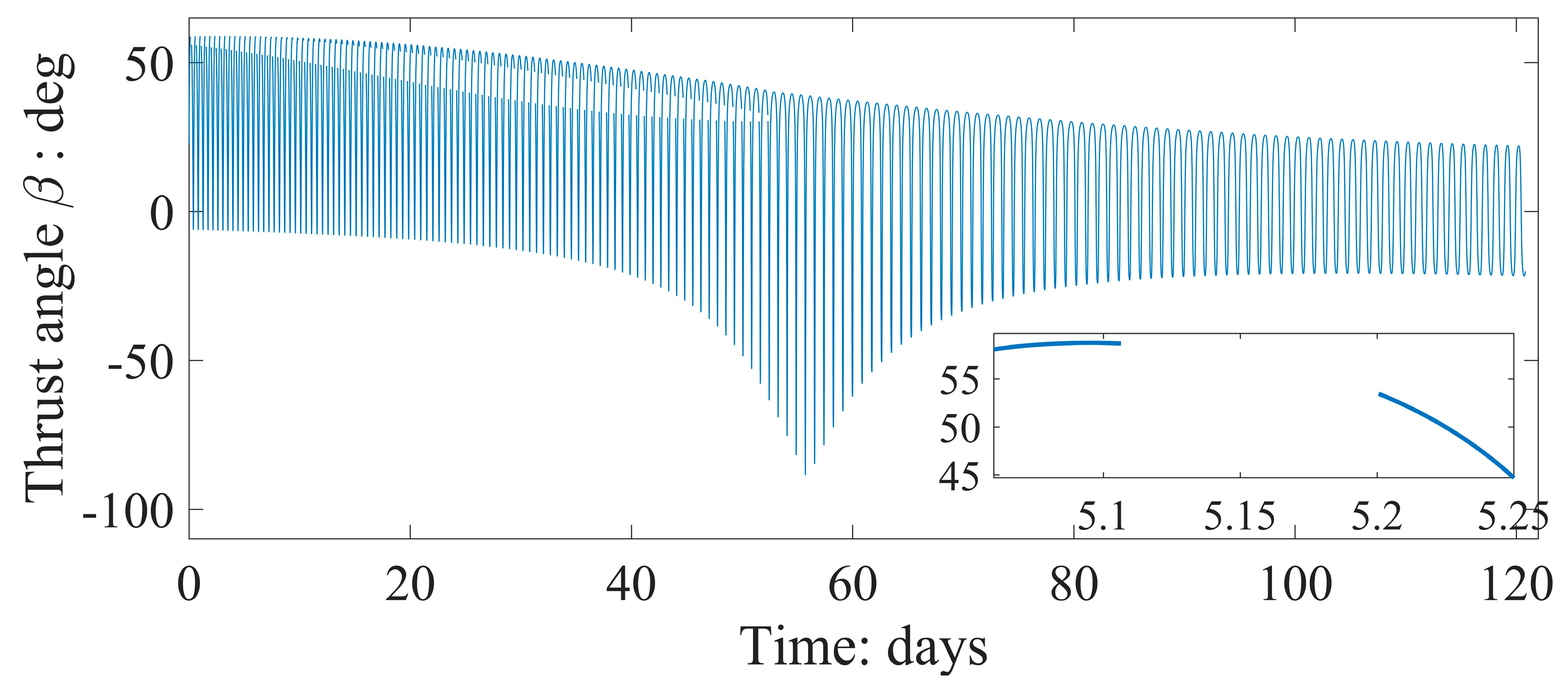
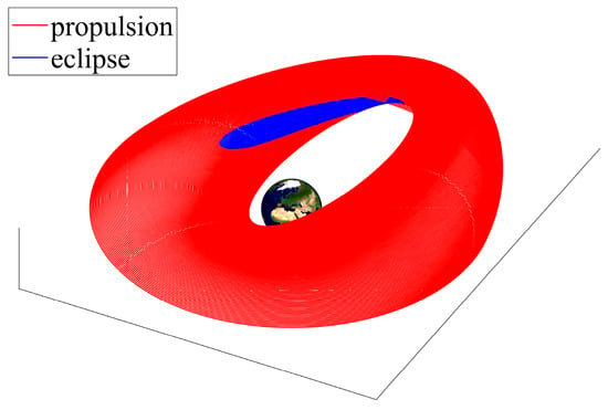
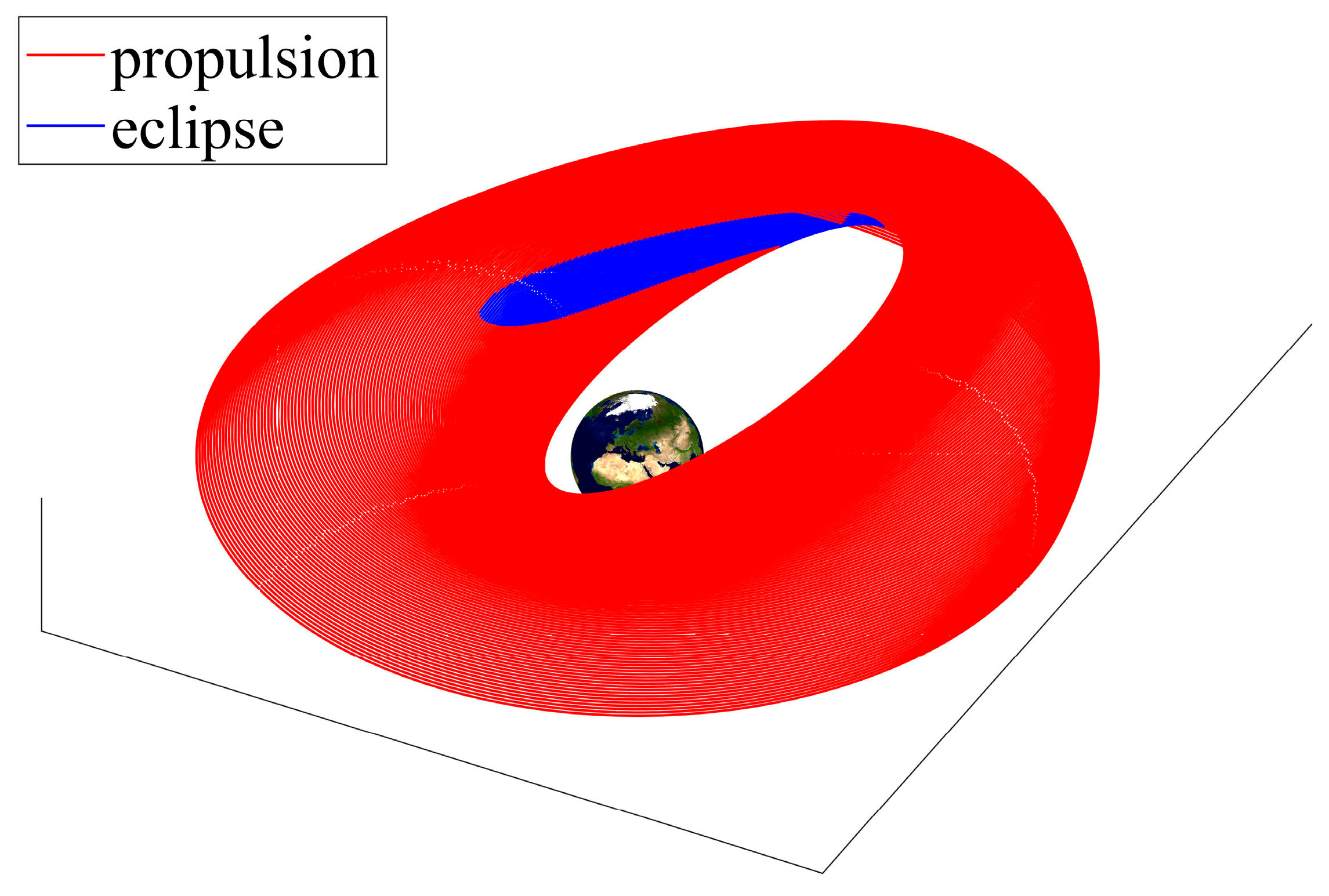
The minimum-time orbit transfer takes 120.82 days, a value close to that found by Kluever through averaging [39], while the final mass ratio is 0.921. Figure 2, Figure 3, Figure 4, Figure 5 and Figure 6 portray the time histories of the osculating semilatus rectum p, eccentricity e, inclination i, and thrust angles. It is worth noting that p, e, and i are constant during eclipses, because the corresponding arcs are Keplerian. Moreover, thrust angles are meaningful only in light arcs, and in fact, blank intervals appear in Figure 5 and Figure 6, associated with eclipse arcs. Finally, Figure 7 illustrates the minimum-time transfer path, with eclipse arcs highlighted in blue.

Figure 2. Time history of the semilatus rectum (with zoom in the inset).

Figure 3. Time history of eccentricity (with zoom in the inset).

Figure 4. Time history of inclination (with zoom in the inset).

Figure 5. Time history of the in-plane thrust angle $\alpha \left(=u_1\right)$ (with zoom in the inset).

Figure 6. Time history of the out-of-plane thrust angle $\beta \left(=u_2\right)$ (with zoom in the inset).

Figure 7. Minimum-time transfer from GTO to GEO (with eclipse arcs in blue).

6. Concluding Remarks

This study addresses multi-arc optimal control problems by considering a very general formulation that also includes intermediate times and states in the objective functional to minimize. This type of problem admits an extended set of necessary conditions, which include multipoint corner relations, to enforce at the junction times between two subsequent arcs. In their general form, these additional conditions do not lead to a closed-form solution for the jump relations of the costate variables at the junction times (with the remarkable exception of class C). Yet, this work shows that 16 cases can occur for the multipoint corner conditions and groups them into three classes. For each of them, closed-form, explicit solutions of the multipoint corner relations are identified, if certain conditions are met. This allows for the sequential solution of multi-arc optimal control problems, which is very advantageous, especially in the presence of a large number of arcs. In fact, in the context of indirect solution approaches, if corner conditions are solvable sequentially, then a parameter set can be identified that retains the reduced size of the typical set associated with a single-arc optimization problem. As a result, the exact fulfillment of the multipoint corner conditions is accompanied by an additional advantage of a computational nature.

Two challenging aerospace trajectory optimization problems are analyzed as illustrative cases of practical interest, i.e., (i) the minimum-fuel ascent path of a multistage launch vehicle and (ii) minimum-time low-thrust orbit transfers with eclipse constraints on the available thrust. In both applications, two different sets of state variables are profitably used, and a closed-form sequential solution of the costate jump equations is proven to exist, also leveraging implicit costate transformation. Application (ii) is particularly challenging due to the presence of a large number of arcs, and its numerical solution testifies to the effectiveness of the multi-arc formulation, accompanied by the explicit solution of all necessary conditions at corners.

References

- Berkovitz, L.D.; Medhin, N.G. Nonlinear Optimal Control Theory; CRC Press: Boca Raton, FL, USA, 2013; pp. 177–182. [Google Scholar]
- Bliss, G.A. Lectures on the Calculus of Variations; University of Chicago Press: Chicago, IL, USA, 1946; pp. 187–228. [Google Scholar]
- Bryson, A.E.; Ho, Y.-C. Applied Optimal Control; Ginn and Company: Waltham, MA, USA, 1969; pp. 125–127. [Google Scholar]
- Clarke, F. Functional Analysis, Calculus of Variations and Optimal Control; Springer: London, UK, 2013; pp. 307–318. [Google Scholar]
- Hull, D.G. Optimal Control Theory for Applications; Springer: New York, NY, USA, 2003; pp. 88–102+221–223+275–283. [Google Scholar]
- Leitmann, G. The Calculus of Variations and Optimal Control; Springer Science & Business Media LLC: New York, NY, USA, 1983; pp. 67–70. [Google Scholar]
- Longuski, J.M.; Guzman, J.J.; Prussing, J.E. Optimal Control with Aerospace Applications; Springer: New York, NY, USA, 2014; pp. 105–111+167–174. [Google Scholar]
- Garfinkel, B. Discontinuities in a Variational Problem. Math. Sci. Eng. 1967, 31, 27–62. [Google Scholar]
- Shaikh, M.S.; Caines, P.E. On relationships between Weierstrass-Erdmannn corner condition, Snell’s law and the hybrid minimum principle. In Proceedings of the International Bhurban Conference on Applied Sciences and Technology, IBCAST, Islamabad, Pakistan, 8–11 January 2007; pp. 117–122. [Google Scholar]
- Noble, J.; Schättler, H. Sufficient conditions for relative minima of broken extremals in optimal control theory. J. Math. Anal. Appl. 2002, 269, 98–128. [Google Scholar] [CrossRef] [Scilit]
- Agrachev, A.A.; Biolo, C. Optimality of Broken Extremals. J. Dyn. Control. Syst. 2019, 25, 289–307. [Google Scholar] [CrossRef] [Scilit]
- Osmolovskii, N.P. On Second-Order Necessary Conditions for Broken Extremals. J. Optim. Theory Appl. 2015, 164, 379–406. [Google Scholar] [CrossRef] [Scilit]
- Osmolovskii, N.P.; Maurer, H. Second-order optimality conditions for broken extremals and bang-bang controls: Theory and applications. Springer Optim. Its Appl. 2016, 109, 147–201. [Google Scholar]
- Garavello, M.; Piccoli, B. Hybrid Necessary Principle. SIAM J. Control. Optim. 2005, 43, 1867–1887. [Google Scholar] [CrossRef] [Scilit]
- Clarke, F.H.; Vinter, R.B. Optimal Multiprocesses. SIAM J. Control Optim. 1989, 27, 1072–1091. [Google Scholar] [CrossRef] [Scilit]
- Dmitruk, A.V.; Kaganovitch, A.M. Maximum Principle for Optimal Control Problems with Intermediate Constraints. Comput. Math. Model. 2011, 22, 180–215. [Google Scholar] [CrossRef] [Scilit]
- Bressan, A.; Hong, Y. Optimal Control problems on Stratified Domains. Netw. Heterog. Media 2007, 2, 313–331. [Google Scholar] [CrossRef] [Scilit]
- Bhattacacharya, R.N.; Bhattacharjee, M. Modification of Weierstrass-Erdmann corner conditions in space navigations. AIAA J. 1964, 2, 1145–1147. [Google Scholar] [CrossRef] [Scilit]
- Miele, A. General variational theory of the flight paths of rocket-powered aircraft, missiles and satellite carriers. Astronautica Acta 1959, 4, 264–288. [Google Scholar]
- Clarke, F.H.; Vinter, R.B. Applications of Optimal Multiprocesses. SIAM J. Control Optim. 1989, 27, 1048–1071. [Google Scholar] [CrossRef] [Scilit]
- Pontani, M. Optimal Space Trajectories with Multiple Coast Arcs Using Modified Equinoctial Elements. J. Optim. Theory Appl. 2021, 191, 545–574. [Google Scholar] [CrossRef] [Scilit]
- Pontani, M.; Corallo, F. Optimal low-thrust lunar orbit transfers with shadowing effect using a multiple-arc formulation. Acta Astronaut. 2022, 200, 549–561. [Google Scholar] [CrossRef] [Scilit]
- Pontani, M.; Corallo, F. Optimal Low-Thrust Earth Orbit Transfers with Eclipses Using Indirect Heuristic Approaches. J. Guid. Control. Dyn. 2024, 47, 857–873. [Google Scholar] [CrossRef] [Scilit]
- Krantz, S.G.; Parks, H.R. The Implicit Function Theorem. History, Theory, and Applications; Springer: New York, NY, USA, 2013; pp. 41–48. [Google Scholar]
- Prussing, J.E.; Conway, B.A. Orbital Mechanics; Oxford University Press: New York, NY, USA, 2013; pp. 13–19+46–53+101–117. [Google Scholar]
- Pontani, M. Advanced Spacecraft Dynamics; Efesto: Rome, Italy, 2023; pp. 251–268. [Google Scholar]
- Vinh, N.H.; Busemann, A.; Culp, R.D. Hypersonic and Planetary Entry Flight Mechanics; The University of Michigan Press: Ann Arbor, MI, USA, 1980; pp. 19–28. [Google Scholar]
- Pontani, M. Particle swarm optimization of ascent trajectories of multistage launch vehicles. Acta Astronaut. 2014, 94, 852–864. [Google Scholar] [CrossRef] [Scilit]
- Aziz, J.; Scheeres, D.; Parker, J.; Englander, J. A Smoothed Eclipse Model for Solar Electric Propulsion Trajectory Optimization. Trans. Jpn. Soc. Aeronaut. Space Sci. 2019, 17, 181–188. [Google Scholar] [CrossRef] [Scilit]
- Bastante, J.C.; Letizia, F.; De Bruijn Bastante, F.J.C.; Letizia, F.; De Bruijn, F.; Lubke-Ossenbeck, B. Application of the Sequential Gradient Restoration Algorithm to the Solution of the Low Thrust Transfer Problem. Aerotec. Missili Spaz. 2017, 96, 228–236. [Google Scholar] [CrossRef] [Scilit]
- Ferrier, C.; Epenoy, R. Optimal Control for Engines with Eletro-Ionic Propulsion Under Constraint of Eclipse. Acta Astronaut. 2001, 48, 181–192. [Google Scholar] [CrossRef] [Scilit]
- Graham, K.F.; Rao, A.V. Minimum-Time Trajectory Optimization of Low-Thrust Earth-Orbit Transfers with Eclipsing. J. Guid. Control Dyn. 2016, 53, 289–303. [Google Scholar] [CrossRef] [Scilit]
- Mazzini, L. Finite Thrust Orbital Transfers. Acta Astronaut. 2014, 100, 107–128. [Google Scholar] [CrossRef] [Scilit]
- Pontani, M. Optimal Low-Thrust Trajectories Using Nonsingular Equinoctial Orbit Elements. Adv. Astronaut. Sci. 2020, 170, 443–462. [Google Scholar]
- Singh, S.K.; Taheri, E.; Woollands, R.; Junkins, J. Mission Design for Close-Range Lunar Mapping by Quasi-Frozen Orbits. In Proceedings of the 70th International Astronautical Congress, Washington, DC, USA, 21–25 October 2019. paper IAC-19-C1.1.11. [Google Scholar]
- Battin, R.H. An Introduction to the Mathematics and Methods of Astrodynamics; AIAA Education Series; AIAA: New York, NY, USA, 1987; pp. 448–450+490–494. [Google Scholar]
- Broucke, R.A.; Cefola, P.J. On the Equinoctial Orbit Elements. Celest. Mech. 1972, 5, 303–310. [Google Scholar] [CrossRef] [Scilit]
- Haberkorn, T.; Trélat, E. Convergence Results for Smooth Regularizations of Hybrid Nonlinear Optimal Control Problems. SIAM J. Control Optim. 2011, 49, 1498–1522. [Google Scholar] [CrossRef] [Scilit]
- Kluever, C.A. Low-Thrust Trajectory Optimization Using Orbital Averaging and Control Parameterization. In Spacecraft Trajectory Optimization; Cambridge University Press: New York, NY, USA, 2010; pp. 112–138. [Google Scholar]
Disclaimer/Publisher’s Note: The statements, opinions and data contained in all publications are solely those of the individual author(s) and contributor(s) and not of MDPI and/or the editor(s). MDPI and/or the editor(s) disclaim responsibility for any injury to people or property resulting from any ideas, methods, instructions or products referred to in the content. |
© 2025 by the author. Licensee MDPI, Basel, Switzerland. This article is an open access article distributed under the terms and conditions of the Creative Commons Attribution (CC BY) license (https://creativecommons.org/licenses/by/4.0/).