Article

Risk Prediction of Shipborne Aircraft Landing Based on Deep Learning

1
School of Economics and Management, Beihang University, Beijing 100191, China
2
The Second Academy, Naval Aviation University, Yantai 264001, China
*
Author to whom correspondence should be addressed.
Aerospace 2025, 12(10), 922; https://doi.org/10.3390/aerospace12100922 (registering DOI)
Submission received: 3 August 2025 / Revised: 30 September 2025 / Accepted: 1 October 2025 / Published: 13 October 2025
(This article belongs to the Section Aeronautics)

Abstract

Shipborne fighters play a critical role in far-sea operations. However, their landing process on aircraft carrier decks involves significant risks, where accidents can lead to substantial losses. Timely and accurate risk prediction is, therefore, essential for improving flight training efficiency and enhancing the combat capability of naval aviation forces. Machine-learning algorithms have been explored for predicting landing risks in land-based aircraft. However, owing to the challenges in acquiring relevant data, the application of such methods to shipborne aircraft remains limited. To address this gap, the present study proposes a deep learning-based method for predicting landing risks of shipborne aircraft. A dataset was constructed using simulated ship movements recorded during the sliding phase along with relevant flight parameters. Model training and prediction were conducted using up to ten different input combinations with artificial neural networks, long short-term memory, and transformer neural networks. Experimental results demonstrate that all three models can effectively predict landing parameters, with the lowest average test error reaching 3.5620. The study offers a comprehensive comparison of traditional machine learning and deep learning methods, providing practical insights into input variable selection and model performance evaluation. Although deep learning models, particularly the Transformer, achieved the highest accuracy, in practical applications, the support of hardware performance still needs to be fully considered.

1. Introduction

Shipborne aircraft are a vital component of naval infrastructure. Compared with other operational tools, they possess the unique ability to rapidly enter and exit battlefields and execute efficient strikes against air, surface, underwater, and ground combat targets. The primary distinguishing feature of shipborne aircraft that sets them apart from land-based aircraft is their landing platform, the aircraft carrier deck. This uniqueness poses considerable challenges, and among all the operational phases of shipborne aircraft, the landing stage has the highest hazard coefficient and is the most accident-prone. According to empirical data, 80% of shipborne aircraft accidents occur during landing [1]. Therefore, investigating the safety of the landing process has substantial theoretical and practical importance.
Extensive studies have been conducted to address this issue. Bobylev et al. [2] studied the effects of airflow fields and weather on aircraft safety across four dimensions: ship wake-simulation devices, multi-aircraft interaction effects, airflow disturbance effects, and the decomposition and analysis of airflow disturbances. The results, validated through wind tunnel and real-aircraft testing, revealed key airflow disturbance characteristics and identified critical safety distance thresholds during landing. Bayen et al. [3] applied optimal control theory and the level set method to investigate the automatic landing safety of high-dimensional aircraft models. They proposed a numerical method to calculate the reachable set of hybrid systems and derived both the maximum controllable invariant set and a corresponding control law to ensure that the ship remains within a safe state space, thereby guaranteeing aircraft safety.
In recent years, with the advancement of aircraft carrier capabilities in China, studies in the country have focused on shipborne aircraft landing safety. Tian and Zhao [4] introduced a safety-oriented multidimensional state-space modeling approach for shipborne aircraft landing missions. They established nonlinear relationships between system state representation data and landing safety features. Moreover, they employed multivariate statistical techniques to reduce dimensionality, and ultimately constructed a numerical model linking independent variables to landing safety. Wang et al. [5] focused on the adaptability of shipborne aircraft, analyzed the influence of both aircraft and environmental factors on safety, and quantitatively determined the minimum deck length for safe escape. Li and Zhao [6] developed a safety model for shipborne aircraft approach and landing by integrating human, machine, and system loop factors using a fuzzy control approach. They evaluated the influence of safety factors through simulation. Yang et al. [7] extended the multidimensional state-space model for landing by incorporating actual landing data from F-18 shipborne aircraft. They further analyzed the data using Bayesian methods and proposed a method to assess the landing status of shipborne aircraft.
Ship-landing safety control strategies are generally categorized into two types: Landing Signal Officer (LSO)-assisted decision-making and automatic landing systems. In recent years, several studies on fully automatic shipborne aircraft landing have been conducted in China. Zhu et al. [8,9,10] and Jiang et al. [11] explored the design of longitudinal and transverse guidance laws, compensation of deck-motion compensation, and suppression of ship wake disturbances using predictive control and sliding mode variable structure approaches [12,13,14,15]. Additionally, combinations of sliding mode variable structures with fuzzy proportional–integral–derivative control and intelligent control algorithms have been employed to improve control performance [16,17,18]. However, research on automatic landing systems in China has been largely theoretical, and practical implementation is yet to progress.
At present, shipborne aircraft landings primarily rely on LSOs to provide auxiliary guidance to pilots to enhance safety. With ongoing technological advancements, the equipment used by LSOs has become increasingly diverse. Anti-jamming radios and video-based head-up displays (HUDs) offer more accurate information to support LSO decision-making. Several tools and their operational principles, such as optical aid systems and video HUDs, as well as shore-based landing-aid and manually operated visual assistance systems have also been adopted. Although these tools enhance decision-making efficiency, the final judgment still relies heavily on the subjective assessment of the LSO. Furthermore, there remains substantial potential for improving timeliness and accuracy beyond the general outline of present and future risks provided by existing systems.
Owing to technological advancements, aircraft recording equipment now provide more comprehensive and accurate flight data. Simultaneously, improvements in computer performance have enabled the application of Machine Learning (ML) methods [19] to process these data; uncover hidden information; and identify, reduce, and prevent flight risks, thereby enhancing operational safety. Considerable progress has been made in the control and risk-prediction of land-based aircraft during landing. Puranik et al. [20] utilized a Random Forest (RF) algorithm to predict vacuum and ground velocities during aircraft landing based on flight parameters from the approach phase. Compared with existing methods, their approach offered greater accuracy and faster processing, enabling sufficient time for flight decision-making. The model demonstrated robustness across different aircraft types and airports.
To evaluate the structural performance of aircraft landing gear, Xu [21] developed a neural network model to predict the vertical load on the landing gear at the 100% limit sinking speed. The approach enhanced test-point accuracy and offered a novel method for studying landing gear strength. Given that flight data are sequential, Wang et al. [5] employed a Long Short-Term Memory (LSTM) network to model long-term dependencies and predict vertical landing velocity. They used Bayesian inference to convert network outputs into probabilistic distributions. Experimental results confirmed the robustness of the model across different aircraft types and airport environments. Although most studies predominantly use numerical predictors, ML is also applicable to classification tasks. Zhang et al. [22] examined the proportional relationship between offset center distance and lateral landing risk. They further constructed a transformation function using a Back Propagation (BP) neural network, and defined risk levels based on threshold values. Ni et al. [23] used an ensemble learning approach, combining deep neural networks and Support Vector Machine (SVM) to process both numerical and textual variables in imbalanced flight data (e.g., aviation summaries). They classified events into five risk levels and built a decision support system to assist analysts in examining incidents, thereby helping risk managers quantify landing risks, prioritize actions, allocate resources, and implement proactive safety strategies [22].
As with land-based aircraft, shipborne flight data comprise numerous parameters recorded at high frequency. Effectively mining the hidden information within these data can enable the identification of risks and their influencing factors, thereby shifting risk management from passive response to proactive prevention [24]. Conventional flight data analysis techniques primarily focus on collecting data from onboard recorders, retrospectively analyzing flight data records, identifying anomalies, designing and implementing corrective measures, and evaluating their effectiveness. Although this approach contributes to flight safety management, it relies on prior knowledge from past flights and lacks adequate timeliness, as it cannot provide real-time analysis of current flight conditions.
Compared with conventional data analysis methods, ML techniques, particularly Deep Learning (DL), offer substantial advantages in terms of prediction accuracy and processing speed. They effectively manage large-sample multivariable flight data, predict ship-performance indicators, identify factors affecting safety, and support risk management. Studies worldwide have applied these techniques to shipboard landing risk management. Li [25] used neural networks to predict the risk of shipborne aircraft landings and analyze related factors affecting ship safety, thereby establishing a control model for landing operations. Experimental results indicated that variables such as velocity and disturbance sinking rate significantly influence LSO decision-making, and risk areas during return flights can be classified based on decision-making time frames.
ML methods have also been applied to establish a nonlinear mathematical relationship between time-related factors and landing safety. Studies have explained the principle of minimizing risk during the landing process using event tree models, where the target is defined as the tree root and events as branch leaves, enabling detailed analysis of event risk levels [4,26]. Brindisi and Concilio [27] employed probabilistic and regression neural networks to develop a comfort model for pilots during shipboard operations, emphasizing the subjective nature of comfort.
However, in China, research in this area remain relatively limited. Xiao et al. [28] performed dimensionality reduction through principal component analysis of helicopter landing data, eliminating variable correlations, and subsequently entered the reduced data into a BP neural network to predict helicopter landing loads. Experimental results revealed that their method could technically support the evaluation of landing loads at the edge of the flight envelope and in envelope extension conditions [29]. Tang et al. [30] applied a BP neural network to combine positional elevation deviations obtained from electronic and optical landing systems. Their findings demonstrated the improvement in accuracy of deviation angle signals.
The descent phase of landing usually lasts 20–30 s, and the pilot/LSO needs to make a decision within 3–5 s [15]. So timely and appropriate decision-making is crucial during the landing phase. ML-based data-driven quantitative methods reliably predict future risks associated with shipboard landings, offering valuable tools for real-time monitoring and supporting LSO decisions [31,32]. Therefore, this study employs both conventional machine learning and deep learning algorithms to model and predict the status parameters of shipborne aircraft during the landing phase. Furthermore, while deep learning methods are chosen for their superior capability in capturing complex temporal dependencies in sequential data [33,34], conventional methods such as Gradient Boosting are included as strong baselines to provide a comprehensive performance benchmark and to assess the relative value of more complex models for this specific application.
The remainder of this paper is organized as follows. Section 2 presents the dataset and preprocessing methods, describes the data sources, and explains relevant shipborne indices and modeling theory. It also outlines the structure of each model and the evaluation metrics used. Section 3 presents the experimental results obtained from applying the models to the dataset. Section 4 discusses the findings, and Section 5 summarizes the experimental outcomes and offers scope for future work.

2. Materials and Methods

2.1. Shipborne Aircraft Landing Dataset

2.1.1. Data Source

In this study, flight parameter data were obtained from pilot-operated flight simulator sessions using Digital Combat Simulator World (v2.7), which was conducted for training purposes. The F/A-18 shipborne aircraft was simulated using the Digital Combat Simulator software to perform various mission flights. A total of 505 sorties were recorded, with data sampled at a frequency of 10 Hz. The simulator pilots consisted of both instructors and cadets from the Naval Aviation University. Flight data were exported via TacView (v1.8.0) software and compiled into a dataset in CSV format. The extracted flight parameters included velocity, altitude, and pitch and roll angles. Although the simulator provides high-fidelity aerodynamic and deck motion modeling, it should be noted that simulated data may not fully capture all real-world variabilities such as extreme weather conditions or emergency scenarios. This limitation should be considered when generalizing the model to actual operations.

2.1.2. Description of Key Variables

The spatial parameters, which reflect the current three-dimensional position of the shipborne aircraft, include the longitude, latitude, and altitude of the aircraft. The landing phase of a shipborne aircraft focuses more on the relative position between the aircraft and the carrier deck than on absolute geographical coordinates; therefore, a coordinate system was defined with the center of the carrier deck as the origin. The latitude and longitude of the aircraft were converted into relative positional coordinates of the form (x, y); the height of the aircraft was represented by the z coordinate. Hence, the spatial position of the shipborne aircraft at any given moment was described by a set of three-dimensional variables (x, y, z).
The attitude of the aircraft, which indicates the orientation of the aircraft during flight, is represented by attitude angles, including pitch, roll, and heading angles. A body-fixed coordinate system was established with the center of mass ‘O’ of the aircraft as the origin (Figure 1). The axis x b pointed forward along the longitudinal axis of the aircraft structure; the axis z b lay in the plane of symmetry and was perpendicular to x b ; the axis y b pointed to the right and was perpendicular to the plane of symmetry. Based at point O, a geodetic coordinate system fixed to the aircraft was defined with the axis z b g pointing vertically downward and the horizontal plane at this position containing the x b g and y b g axes, which were determined using the right-hand rule.
In this coordinate system, the heading angle (denoted as φ) was defined as the angle between the projection of x b on the horizontal plane x b g y b g , and the axis x b g , indicating the pilot’s directional control. The pitch angle (denoted as θ) was defined as the angle between x b and the plane x b g y b g , representing the pilot’s control over the aircraft’s vertical attitude. The roll angle (denoted as ∅) was defined as the angle between the plane x b z b and the vertical plane x b , representing the pilot’s ability to control horizontal attitude adjustments.

2.2. Evaluation Models

This section introduces the DL models employed in this study and outlines the evaluation metrics used to assess their performance. It also explains the architecture and unique characteristics of each model.

2.2.1. Artificial Neural Network

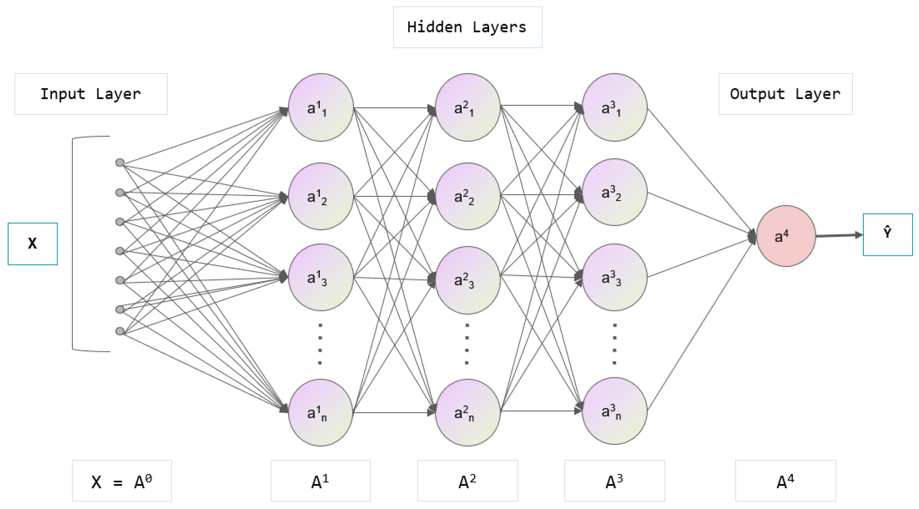
The ANN, also known as a connectionist model, is a mathematical framework for distributed parallel information processing that simulates the behavior of animal neural networks. Leveraging the complexity of interconnected systems, an ANN processes information by dynamically adjusting the connections among a large number of internal nodes (Figure 2).
The ANN mainly comprises three layers: input, hidden, and output layers. The input layer accepts a one-dimensional vector and feeds each component into the network. The hidden layer forms the core of the network and can consist of multiple layers (the example in Figure 2 includes three hidden layers). The output layer—the final layer—generates the model’s prediction results.
Each circle in the diagram represents a basic unit of the ANN (called a neuron), which interacts with other neurons through a predefined connection structure. This design simulates the operational principle of biological neural networks. In a fully connected layer, every neuron in one layer is connected to every neuron in the subsequent layer, as indicated by the arrows in Figure 2.
During the training phase, information flows from the input neurons through the hidden layers to the output layer. The difference (loss) between the predicted result and actual target value is then propagated backward from the output layer to the input layer. This backward propagation process updates the network parameters.

2.2.2. Long Short-Term Memory Network

Shipboard landing data exhibit strong temporal characteristics, meaning that the state of the aircraft (such as position, velocity) at any given moment is highly dependent on its state in the previous moments.
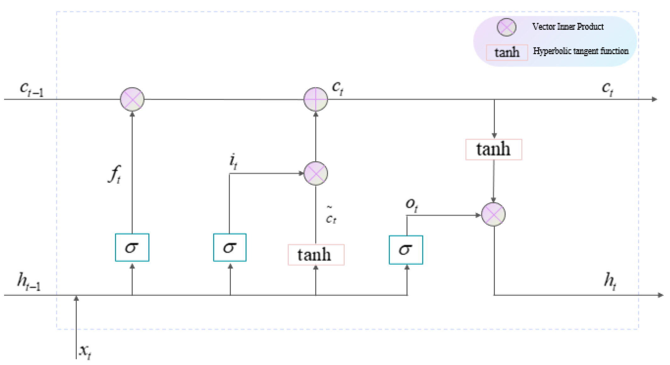
The LSTM is a type of recurrent neural network (RNN) specifically designed for processing and predicting time-series data. It was employed in this study for modeling purposes because shipboard landing data exhibit strong temporal characteristics and involve specific time intervals between key points. The most notable feature of LSTM is the incorporation of memory cells and gating mechanisms between hidden neurons, which enables the network to retain historical information and maintain long-term dependencies. Standard RNNs often face recurring problems of vanishing and exploding gradients when processing sequential data. The LSTM effectively addresses these problems through its memory cell and gating mechanisms. The structure of the LSTM model is illustrated in Figure 3.
In Figure 3, the time step is denoted as t, the input vector as x t , the output as h t , and the memory cell as c t . The input vector first passes through the forget gate f t , where Equation (1) determines which information to discard. In the second stage, the input passes through the input gate i t , and Equation (2) is used to determine which new information should be stored. Finally, the output gate o t uses Equation (3) to determine the output value.
f t = s i g m o i d ( W x f x t + W h f h t 1 + b f ) s i g m o i d ( x ) = 1 1 + e x
i t = s i g m o i d ( W x i x t + W h i h t 1 + b i ) c ~ t = t a n h ( W x c x t + W h c h t 1 + b c ) c t = f t * c t 1 + i t * c ~ t
o t = s i g m o i d ( W x o x t + W h o h t 1 + b o ) h t = o t * t a n h ( c t )

2.2.3. Transformer

The Transformer is a DL model originally developed for natural language processing and other sequence-to-sequence tasks. Its key innovation is the introduction of the self-attention mechanism, which enables simultaneous consideration of all the positions in the input sequence. This capability enables the Transformer to capture both long- and short-term dependencies within a sequence. Owing to these advantages, the Transformer model was applied in this study to model time-sequential shipboard landing data.
The structure of the Transformer is illustrated in Figure 4. It mainly comprises two blocks: the encoder and decoder blocks. The encoder block encodes the input sequence and is composed of N stacked encoders (N = 6). Each encoder includes multi-head attention, a fully connected feedforward network, and residual connections. The decoder block decodes the encoded output to generate the final prediction result. It comprises six stacked decoders, each of which adds a masked self-attention module to prevent the model from attending to future positions during training.
Notably, variables must undergo positional encoding before being fed into either the encoder or decoder blocks. Without positional encoding, the model treats input elements (e.g., word or features) as unordered, which is not appropriate for sequential data. By incorporating positional information, the model captures the relative and absolute order of elements in the sequence, enabling it to better learn the semantic structure and temporal relationships within the data.

2.2.4. Traditional Machine Learning Baseline Models

To provide a comprehensive performance benchmark for the deep learning models, three widely used traditional machine learning algorithms—RF, Gradient Boosting Machine (GBM), and Support Vector Regression (SVR)—were implemented as baseline models. These models were chosen for their strong performance in regression tasks and their ability to handle nonlinear relationships in tabular data.
RF: an ensemble method that constructs multiple decision trees during training and outputs the average prediction of the individual trees. It is robust to overfitting and capable of capturing complex interactions among features.
GBM: a boosting technique that builds trees sequentially, where each new tree corrects the errors of the previous one. It often achieves high predictive accuracy.
SVR: a kernel-based method that seeks to find a hyperplane that best fits the data within a specified margin of error. It is effective in high-dimensional spaces.
The key hyperparameters for three ML models, along with their descriptions, are summarized in Table 1.

2.2.5. Evaluation Indices

To evaluate the performance of the model and update parameters through BP during training, it is necessary to define both appropriate evaluation metrics and a loss function. As this study addressed a regression problem, the mean absolute error (MAE) e M A E was selected as the loss function during training and as the evaluation metric for model performance. The e M A E expression is given in Equation (4), where m denotes the number of samples, y i represents the true value of each sample, and y i ^ denotes the corresponding predicted value. A lower e M A E value indicates better predictive accuracy.
e M A E = 1 m i = 1 m | y i y i ^ |
This article integrates the errors of various predictive indicators, representing the overall accuracy error of the model; it is assumed that all indicators are equally important. In the future, more suggestions from LSO can be collected to assign corresponding weights to the importance of each indicator, thereby achieving a more refined predictive system.

3. Experiments

3.1. Data Preprocessing

The data were cleaned and preprocessed to ensure their format aligned with the model’s input requirements. First, the flight landing stage data were extracted based on specific indicators. Second, the independent and dependent variables used in the model were identified, following which the input feature and prediction vectors were constructed. Finally, the data were cleaned by removing irrelevant variables and addressing missing or abnormal values through manual techniques and ML methods.
The sensors started recording data immediately from system start-up. The data captured included the entire simulated flight training process. This study focused specifically on the sliding phase of shipboard landing, which necessitated isolating the relevant segment based on appropriate discrete indicators. The key evaluation criteria for shipboard landing were identified based on existing literature. Among the three recognized aircraft landing mode classes (I–III), the simulator recorded Class I data. The landing path was not a straight descent; rather, it followed a “spiral progressive” trajectory. Specifically, it was described as “three legs, four turns,” where the aircraft began a turn approximately 30 s after crossing the ship’s island, aligning with the ship’s heading.
During the landing process, the aircraft maintained an attack angle of approximately 11°, calculated from the attitude angle. In the sliding phase, pilots adhered to the strategy of “looking at the light, aligning, and maintaining angle.” The ideal sliding trajectory was a straight line relative to the aircraft carrier deck. Using time, altitude, angle of attack, and vertical velocity data, the flight data were segmented to extract the portion corresponding to the sliding phase.
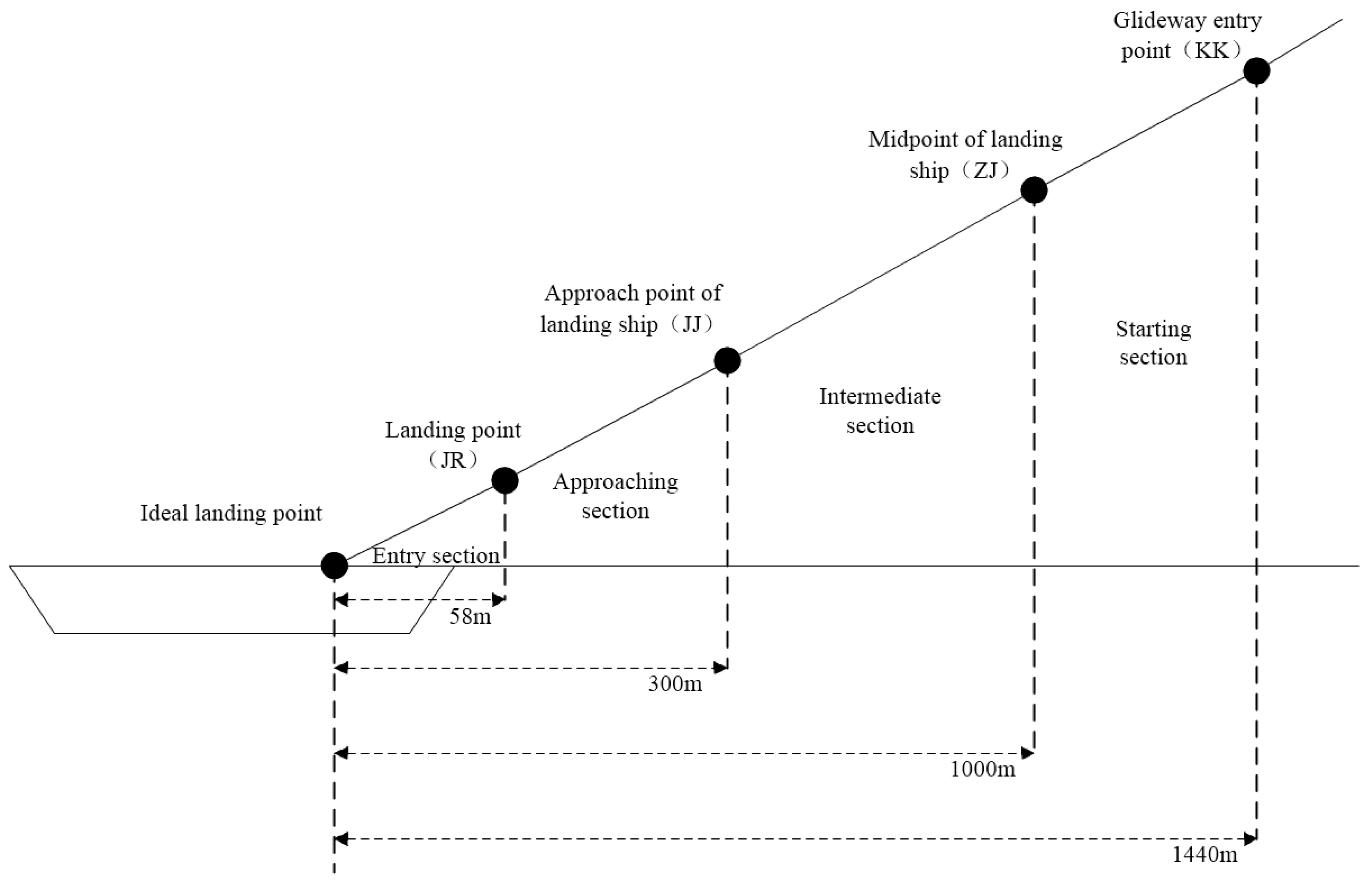
Owing to variability in landing times across different sorties and the use of fixed-interval sensor sampling, variations existed in the data length for each flight. To address this and ensure uniform vector length for model input, the sliding phase was standardized based on the relative distance between the aircraft and key ship positions. Four characteristic points were selected as landmarks for segmenting the landing trajectory: the entry point of the sliding track (KK), the midpoint of the landing path (ZJ), a mid-to-late phase marker (JJ), and the actual touchdown point (JR). These four key assessment points for shipboard landing are illustrated in Figure 5.
The dataset originally contained 18 variables, resulting in high dimensionality that increased computational resource consumption during model training. Additionally, the variable set included independent variables such as aircraft shelf number and pilot code. Some samples exhibited missing or abnormal values owing to equipment testing errors or early termination of recordings. Therefore, data cleaning was necessary.
The cleaning process began with manual inspection to identify and eliminate irrelevant variables, reducing the number of variables from 18 to 13. In handling outliers and missing values, samples with more than 30% anomalous data were discarded. When the proportion of missing or abnormal values was below 30%, interpolation was performed using the average of the two adjacent recorded points. After preprocessing, there were 436 valid samples.
For the four characteristic points identified in the previous section, the 13 variables obtained after dimension reduction were used as the key feature parameters for predicting ship landing risks. Additionally, four variables related to the moment the aircraft’s tail hook engaged the arresting gear were selected. Among them, ZX and ZY represent the positions of the carrier-based aircraft’s tail hook on the aircraft carrier’s deck arrestor wire, reflecting the lateral and longitudinal deviations of the landing position; ZAS and ZRFR represent the speed inertia of the carrier-based aircraft during landing, reflecting the sinking rate deviation at the time of landing. They all have a significant impact on landing risks. For example, when the lateral deviation ZX during landing is too large, it indicates that the carrier-based aircraft’s touchdown point is too far to the right/left (the standard landing should be aligned with the center-line of the carrier’s deck), which may cause the aircraft to overshoot the deck during landing; also, if the sink rate of the carrier-based aircraft is too high, it will greatly increase the risk of the aircraft’s tail striking the front deck of the carrier. Details of each feature are presented in Table 2.
The RF algorithm was employed to rank the importance of the 13 variables retained after manual screening. RF is an ensemble learning method that uses the bagging approach to combine decision trees for improved prediction performance. It involves randomly sampling data to train each tree and randomly selecting features at each node to determine the optimal split. One key application of RF is ranking the importance of input variables. Feature importance is assessed by calculating the average reduction in Gini purity across all tree nodes where the feature is used.
There were four prediction targets (Table 2). A separate RF model was trained for each target. The number of decision trees was set to 100, and each tree was trained on a maximum of 128 samples. Table 3 presents the significance scores of each characteristic variable with respect to each prediction index. The final column in the table presents the average importance score of each variable across all four targets. The variables were ranked in descending order based on these average scores. The top nine variables, highlighted in bold in Table 3, were selected for further analysis.
Through further screening of characteristic variables using the RF algorithm, nine flight parameters at four feature points were selected as the input data for the subsequent models. These inputs were represented by matrix A, and the prediction vectors were denoted as B, as shown in Equation (5). Considering that the scales of the four predictor variables are different, where ZX and ZY are 10−1, and ZAS and ZRFR are 101, the scales will be unified when calculating MAE, as detailed in Equation (6). In addition, to more intuitively reflect the difference between the model’s predicted values and the actual values, the Mean Absolute Error Proportion (MAEP) is used, which allows for a better vertical comparison between the predicted values and the actual values, as detailed in Equation (7).
A = X K K A S K K A A K K R F R K K A P K K R A K K C A K K H T A K K D C A K K X Z J A S Z J A A Z J R F R Z J A P Z J R A Z J C A Z J H T A Z J D C A Z J X J J A S J J A A J J R F R J J A P J J R A J J C A J J H T A J J D C A J J X J R A S J R A A J R R F R J R A P J R R A J R C A J R H T A J R D C A J R
B = [ Z X , Z Y , Z A S , Z R F R ]
M A E = 1 4 [ M A E _ Z A S + M A E _ Z R F R + 10 * ( M A E _ Z X + M A E _ Z Y ) ]
M A E P i = 1 m i j = 1 m i ( | y j y j y j | ) * 100 % , i = Z X , Z Y , Z A S , Z A R F M A E P = 1 4 * i M A E P i

3.2. Model Training and Reasoning

This section presents the results of model training and prediction. The hardware specifications used for the experiments are listed in Table 4. Python (v 3.10.4) was used as the programming language, with PyTorch (v 12.6) selected as the DL framework.
The preprocessed dataset was divided into training, validation, and test sets in a 7:2:1 ratio. The relevant hyperparameter settings used during model training are listed in Table 5. The model was trained for 200 epochs, with a batch size of 64. The initial learning rate was set to 0.01, and the Adam optimizer was used to update the training parameters during the BP phase.
It is reasonable to assume that the closer a point is to the landing point, the more accurate the prediction will be. However, at closer distances, pilots have less time to make necessary adjustments. Hence, this study compared models using combined input modes—for example, a model trained with input from point KK alone versus one trained with combined inputs from points KK and ZJ. Table 6 lists all the input combinations, where combinations 1–4 correspond to individual inputs from each key point, and combinations 5–10 represent combined inputs. For the ANN, ten separate models were trained corresponding to the ten input combinations. As LSTM and Transformer networks account for the temporal nature of the input data, only six combined input configurations were used for training them.
Table 7 presents the architecture of the ANN constructed in this study (using single feature point input as an example). The network comprised three hidden layers. The number of neurons in the input layer was determined by the dimensionality of the input variables. The three hidden layers were fully connected, containing 128, 64, and 32 neurons. The output layer contained four neurons, corresponding to the number of predicted variables. Notably, dropout was applied to the first two fully connected layers, at a rate of 0.2. This means that 20% of the neurons in these layers were randomly deactivated during training—a regularization technique that prevented overfitting.
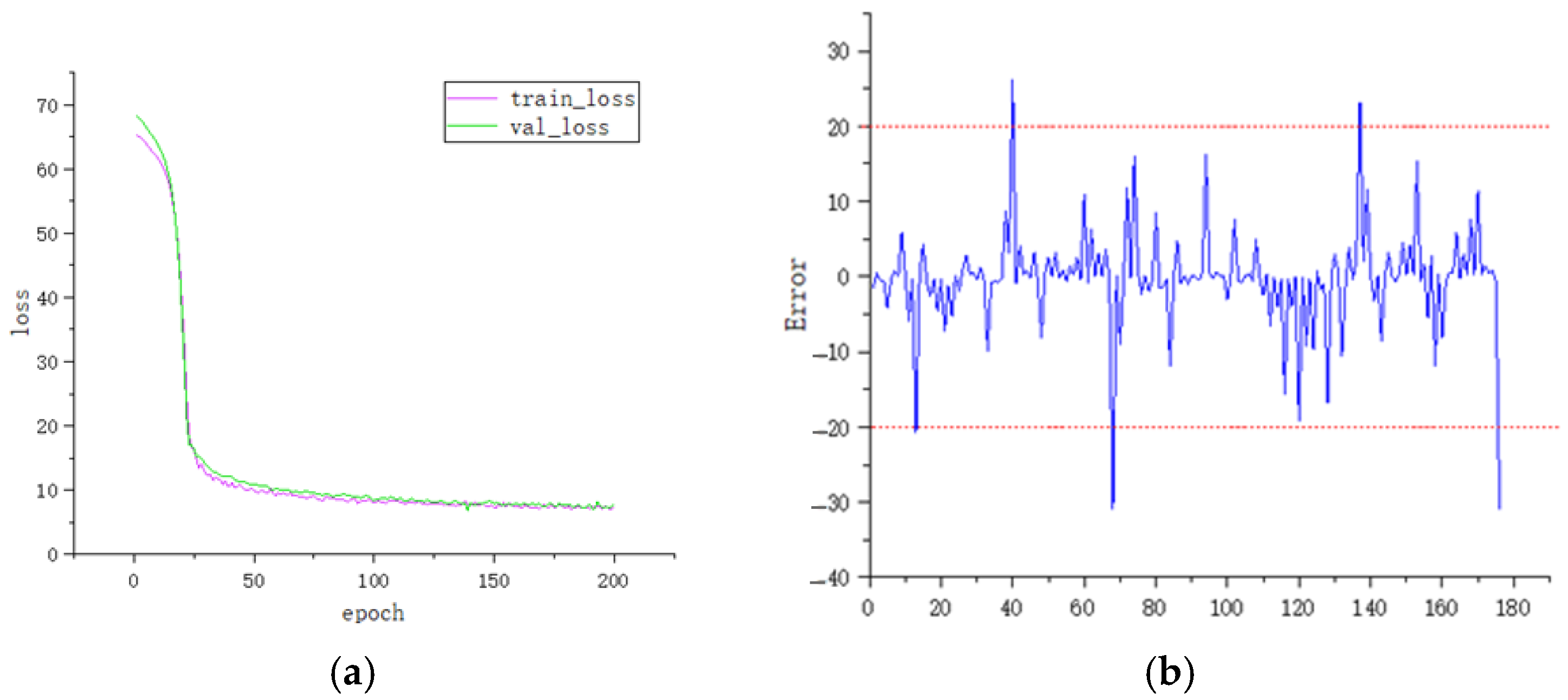
Figure 6 illustrates the loss curves for the training and validation sets during model training using KK as input, as well as the prediction results on the test set after training completion. The training loss curve exhibited a significant drop within the first 25 epochs, and both the training and validation losses stabilized after approximately 100 epochs. Regarding prediction accuracy, 89.78% of the test samples had an error within the range of 10, whereas only 2.84% of the samples exhibited an error exceeding 20. Detailed results for the remaining nine input combinations are provided in Table 8. Among them, the model using JJ + JR as input achieved the best performance in both the training and test phases, with a test set MAE of 4.2039.
The input format supported by LSTM is defined in Equation (8), where n _ s a m p l e s represents the sample size of the input data, t i m e s t e p s denotes the number of time steps per input sample, and n _ f e a t u r e s indicates the number of features at each time step. To fit this structure, the input data were remodeled accordingly. Using two key points as an example, each containing nine features, the time step was set to 2. The input features were divided into two segments, with each time step including nine features. Consequently, the sample feature size was set to 9. This approach was applied similarly to other input configurations.
( n _ s a m p l e s , t i m e s t e p s , n _ f e a t u r e s )
The structure of the LSTM model is detailed in Table 9. The first layer comprised 64 LSTM units, with each unit following the architecture illustrated in Figure 4. To mitigate overfitting, a dropout layer with a rate of 0.2 was applied. The output layer was a fully connected layer with four neurons, corresponding to the four prediction targets.
The training and test results of the LSTM model, using KK + ZJ as the input, are shown in Figure 7. During the training phase, the model loss decreased rapidly within the first 20 epochs, with the rate of decline gradually slowing thereafter. By approximately the 175th epoch, the loss stabilized. In terms of prediction accuracy, 90.9% of the LSTM model’s prediction errors fell within a range of 10. Only 2.27% of the sample errors exceeded 20, indicating slightly better performance than the ANN model. The results for all six input combinations are summarized in Table 10. Among them, the KK + ZJ + JJ + JR input yielded the lowest loss on the training set, and ZJ + JJ + JR achieved the lowest loss on the validation set and the best overall performance on the test set.
The structure of the Transformer model is presented in Table 11, which outlines the output vector dimensions and parameter counts for each layer of the model when two key points are used as input. As the Transformer supports sequential data input, the input format was the same as that used for the LSTM model. Based on the number of key points involved in the ship landing phase, the data were divided into corresponding time steps, with each time step containing nine variables.
The input data first passed two modules: the embedding layer and positional encoding layer (pos_encoder). These layers inserted positional information into the sequence, thus enabling the attention mechanism of the model to recognize the order of the input elements. The embedding layer sets the hyperparameter d mod e l to 64, mapping each feature in each time step into 64-dimensional vectors. Position indices were generated sequentially using natural numbers. Finally, the positional encoding was applied as follows. The even- and odd-numbered dimensions used sine and cosine functions, respectively, as defined in Equation (9), where p o s represents the position index, j represents the dimension index, and d mod e l is fixed at 64.
P E ( p o s , 2 j ) = s i n ( p o s 10000 2 j / d mod e l ) P E ( p o s , 2 j + 1 ) = c o s ( p o s 10000 2 j / d mod e l )
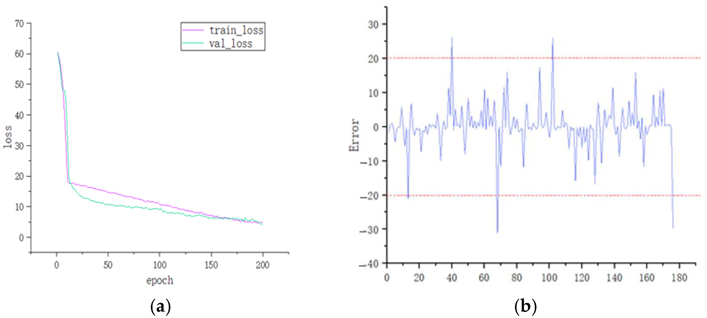
Transformer models were trained and tested using the same six input combinations as the LSTM models. Figure 8 presents the training and test results for the model using KK + ZJ as input. According to the loss curve, the model shows a relatively rapid and balanced decline in loss during the first 140 epochs, after which the loss stabilized. Compared with the ANN and LSTM models, the Transformer converged more slowly; however, it ultimately achieved a lower loss value.
Based on the model’s prediction results, 92.7% of the sample errors fell within a range of 10, whereas only 1.7% exceeded an error of 20. Furthermore, the maximum error was significantly lower than those observed in the ANN and LSTM models. All results are summarized in Table 12. Among all the input configurations, KK + ZJ + JJ + JR yielded the best performance across the training, validation, and test sets.

4. Results

4.1. Comparison of Results of Three Deep Learning Models

The results of the three models were analyzed independently, leading to the following two conclusions:
  • As the number of input key points increased, the loss of the model consistently decreased. This was particularly evident with the LSTM and Transformer models, which are more sensitive to temporal information. Figure 9a compares the prediction accuracy of the LSTM and Transformer models under different input configurations. The loss curve exhibited a negative slope as the number of input points increased. The inclusion of more input variables provided the model with richer information, and the temporal dependency among the key points further enhanced the model’s ability to capture meaningful patterns, thereby improving predictive accuracy.
2.
When the number of input variables was the same, models using key points closer to the landing point achieved higher accuracy. As shown in Figure 9b, for cases with two input key points, the prediction error decreased linearly with the distance between the key points and the landing point. This observation aligns with the hypothesis that key points nearer to the landing point exhibit smoother flight parameter transitions, with a lower likelihood of sharp fluctuations, thus providing more reliable and informative data for accurate prediction.
A comparative analysis was conducted between the best-performing ANN, LSTM, and Transformer models (Table 13). The results indicate that the LSTM and Transformer models outperformed the ANN model owing to their ability to process time series data and capture temporal dependencies among key flight parameters during the landing phase. Both models effectively identified long-range dependencies, establishing connections between information from earlier time steps (i.e., key points farther from the landing) and the final prediction outcomes.
From the perspective of prediction accuracy, the Transformer model achieved the lowest MAE and MAEP among the three. However, in terms of computational cost, the trend was reversed. The ANN model had the fewest parameters, rendering it the most efficient. The LSTM model had approximately 1.5 times more parameters than the ANN model, and the Transformer model had the highest parameter count—143.67 times that of the ANN model.
Table 13 also provides a detailed breakdown of the MAE for each individual prediction target for the best-performing model of each type. This separate analysis is crucial for understanding the specific predictive capabilities for each risk factor. The Transformer model consistently shows the lowest error across all four parameters. Based on the separate MAE values and established safety thresholds, the predicted values can be mapped to risk levels. For example, a longitudinal deviation (ZX) prediction error of <2 m might be considered Low Risk, an error between 2 m and 4 m Medium Risk (requiring minor correction), and an error > 4 m High Risk (potential for missing target wires, suggesting a go-around advisory). Similar thresholds can be defined for lateral deviation (ZY), excessive airspeed (ZAS), and high descent rate (ZRFR). It can transform the prediction regression problem into a classification problem can provide more intuitive references for LSO decision-making.

4.2. Cross-Method Comparative Analysis

To provide a comprehensive benchmark, the proposed deep learning models (ANN, LSTM, Transformer) were compared against the conventional machine learning baselines mentioned in 2.2.4, including RF, GBM, and SVR, and they all use the best-performing input combination (KK + ZJ + JJ + JR).
The hyperparameter values of the three traditional ML models (listed in Table 1) are shown in Table 14. These models were implemented using the scikit-learn library in Python and serve as strong non-deep learning baselines to contextualize the performance gains offered by the more complex ANN, LSTM, and Transformer architectures. All models were trained and tested on the same dataset. The comparison metrics are as detailed in Table 15.
From the comparison, it can be concluded that DL models are generally superior to traditional machine learning models in terms of accuracy and can better handle the complex nonlinear relationships among multiple variables in carrier landing flight parameter data. However, it is worth noting that traditional machine learning models have the advantage of lower hardware computing power requirements. In military application scenarios, LSO sometimes lacks access to a computer that supports the operation of DL models. For scenarios without deployment conditions, the GBM, which achieves the highest accuracy among the three traditional machine learning models, can still be a good choice.

5. Discussion

This study applied DL methods to predict the landing risk of shipborne aircraft. The study comprised two major components. First, data of F/A-18 shipborne aircraft were preprocessed. As the initial step, the sliding phase data of the landing process was extracted. Then, four key landing points—KK, ZJ, JJ, and JR—were identified. During data cleaning, missing and abnormal values were either removed or interpolated. Variables were manually screened, and their importance was ranked using the RF algorithm. Ultimately, nine key flight parameters were retained as characteristic variables.
Second, three DL models—ANN, LSTM, and Transformer—were employed. Up to ten combinations of key input points were used to model aircraft landing risk. Based on the MAE, the results indicate that all three models effectively capture the nonlinear relationships between characteristic and predicted variables. The LSTM and Transformer models’ ability to process temporal data enabled them to better exploit the time-dependent structure of the landing data. For each model, prediction accuracy improved with an increase in the number of input variables. However, more inputs also increased model complexity and demand for computational resources. Additionally, inputs closer to the landing point reduce the time available for LSOs and pilots to make corrective decisions, necessitating a trade-off when selecting input points.
Among the three models, the Transformer model achieved the highest prediction accuracy, but at the cost of significantly greater computational demand. The ANN model, while less accurate, required the fewest parameters and was more resource-efficient. Model selection should balance prediction performance and deployment cost based on practical needs. Furthermore, we compare the accuracy of DL models and three traditional machine learning models. DL models perform better in handling multivariable nonlinear relationships, while traditional machine learning models have the advantage of lower hardware computing power requirements and are easier to deploy in practical applications.
Practical Implications and Usage: This article evaluates the accuracy of the model by predicting four key landing parameters and using the MAE of these four parameters. The experimental results show that the overall prediction error of the model for these landing parameters is within an acceptable range. Therefore, in practical applications, during the descent of carrier-based aircraft, the related flight parameters can be input into the model to obtain predicted landing indicators, thus providing auxiliary decision-making support for LSO.
Limitations and Critical Reflection: While the results are promising, several limitations must be acknowledged. Firstly, the study relies entirely on simulated data. Although the simulator is high-fidelity, it cannot perfectly replicate all nuances of real-world operations, such as extreme atmospheric turbulence, sudden mechanical failures, or the full psychological stress experienced by pilots. Secondly, limited by prior knowledge, this article does not further convert the landing indicators into landing risk values. Therefore, the LSO needs to refer to the predicted values and use prior knowledge to assess the levels of risk and whether to attempt a go-around; for instance, if the predicted lateral deviation exceeds 10 m or the descent rate is above 6 m/s, the system could issue a high-risk warning, suggesting a go-around. Thirdly, the current study predicts parameters, and the translation into a holistic risk assessment, while proposed, requires further validation with operational experts to define robust and accepted threshold values for different risk levels. Finally, the computational complexity of the best-performing model (Transformer) poses a challenge for real-time embedded applications aboard carriers or aircraft, necessitating future work on model optimization and distillation.
Future Work: Future research should focus on several areas: (1) Validating the models using real flight data from shipborne aircraft operations. (2) Further research could combine the expertise of professionals to quantitatively model landing risks, and directly output risk levels based on operational guidelines and expert knowledge, rather than just predicting parameters. (3) By consulting expert opinions, set corresponding weights based on the importance of each indicator, thereby providing a more detailed basis for the overall risk assessment. (4) Implementing a real-time predictive system interface and conducting human-in-the-loop evaluations with experienced LSOs to assess its practical utility and integration into existing workflows.

6. Conclusions

This study developed and compared three deep learning models—Artificial Neural Network (ANN), Long Short-Term Memory (LSTM), and Transformer—for predicting key landing parameters of shipborne aircraft during the critical sliding phase. The models were trained and tested on a dataset derived from high-fidelity flight simulations. The findings demonstrate that deep learning techniques, particularly sequence-aware models like LSTM and Transformer, are highly effective in capturing the complex temporal dynamics of the landing process. The Transformer model achieved the highest prediction accuracy overall, with the lowest mean absolute error, by effectively leveraging its self-attention mechanism to model dependencies across all input key points simultaneously. However, this performance comes at the cost of significantly higher computational complexity compared to the simpler and more efficient ANN.
The study provides a foundational framework for the development of real-time risk prediction systems. By accurately predicting the values of key indicator parameters during the landing phase at the critical glide slope stage of carrier-based aircraft landing, such systems are expected to offer valuable auxiliary decision-making support to LSO, thereby enhancing the safety and efficiency of carrier-based aviation operations. In practical applications, the selection of a model requires a careful trade-off between prediction accuracy, computational latency, and available hardware resources.

Author Contributions

Conceptualization, H.N.; methodology, H.N. and X.D.; software, Z.B.; validation, Z.B. and X.W.; formal analysis, H.N.; investigation, H.N.; resources, Z.B.; data curation, X.W.; writing—original draft preparation, H.N.; writing—review and editing, H.N. and Z.B.; visualization, Z.B.; supervision, X.D.; project administration, X.D. All authors have read and agreed to the published version of the manuscript.

Funding

This research received no external funding.

Data Availability Statement

All data, models, and code generated or used during the study appear in the submitted article.

Conflicts of Interest

The authors declare no conflicts of interest.

Abbreviations

The following abbreviations are used in this manuscript:
LSOLanding Safety Officer
ANNAnimal Neural Network
CAHeading Angle
AAAngle of Attack
RFRRise Rate
APPitch Angle
DCMCenter Deviation Meter
RARoll Angle
HTMHeight Deviation Meter
HTAHigh Deviation
DCACenter Deviation

References

  1. Pervan, B.; Chan, F.C.; Gebre-Egziabher, D.; Pullen, S.; Colby, G. Performance Analysis of Carrier-Phase DGPS Navigation for Shipboard Landing of Aircraft. Navigation 2003, 50, 181–191. [Google Scholar] [CrossRef]
  2. Bobylev, A.V.; Vyshinsky, V.V.; Soudakov, G.G.; Yaroshevsky, V.A. Aircraft Vortex Wake and Flight Safety Problems. J. Aircr. 2015, 47, 663–674. [Google Scholar] [CrossRef]
  3. Bayen, A.M.; Mitchell, I.M.; Oishi, M.M.K.; Tomlin, C.J. Aircraft Autolander Safety Analysis Through Optimal Control-Based Reach Set Computation. J. Guid. Control Dyn. 2007, 30, 68–77. [Google Scholar] [CrossRef]
  4. Tian, J.; Zhao, T. Controllability-involved risk assessment model for carrier-landing of aircraft. In Proceedings of the Annual Reliability and Maintainability Symposium, Reno, NV, USA, 23–26 January 2012. [Google Scholar]
  5. Wang, L.; Zhang, Z.; Zhu, Q.; Jiang, X. Lateral autonomous carrier-landing control with high-dimension landing risks consideration. Aircr. Eng. Aerosp. Tech. 2020, 92, 837–850. [Google Scholar] [CrossRef]
  6. Li, X.; Zhao, Y. Safety simulation analysis of carrier based aircraft entering the ship based on fuzzy reasoning. J. Chin. J. Aeronaut. 2013, 34, 325–333. [Google Scholar]
  7. Liu, F.; Tian, J.; Yang, Q. Safety analysis of carrier based aircraft landing based on Bayes judgment method. J. Syst. Eng. Electron. 2016, 38, 208–214. [Google Scholar]
  8. Zhu, Q. Reference LPV Control of Mixed Yab Model for Landing Side Circuit of Carrier based Aircraft. J. Harbin Eng. Univ. 2013, 34, 83–91. [Google Scholar]
  9. Zhu, Q. Linear variable parameter predictive control of time-varying risk weight matrix for the landing side circuit of carrier based aircraft. J. Control. Theory Appl. 2014, 32, 101–109. [Google Scholar]
  10. Zhu, Q. Design of Longitudinal Landing System Based on Nonlinear Dynamic Inverse Sliding Mode. J. Syst. Eng. Electron. 2015, 36, 2037–2042. [Google Scholar]
  11. Jiang, X.W.; Zhu, Q.D.; Wen, Z.X.; Zhang, Z. Rolling Time Domain Control of Lateral Loop for Carrier based Aircraft Landing. J. Comput. Simul. 2013, 30, 90–93+120. Available online: https://kns.cnki.net/kcms2/article/abstract?v=F0lYaGTXfx_IQt5d7eGwCIyBduZsI5mI2AEUwoKrI4OtKtxP5stYTMazj3dqVuRxkTh9m_qgXaqbWybuKw0adpZLqBfoIF5VU4TkYGFv9g-6CnOYPYFaTHPxjdLVVgX4rUaSAtpmcVtiT4pSdQSiYT-Zc3bHRI4Wuryytd_wjXMPipMhcVDXQF5dOjs6F3QL&uniplatform=NZKPT (accessed on 30 September 2025). (In Chinese).
  12. Zhu, Q.D.; Meng, X.; Zhang, Z. Longitudinal Landing System Design Based on Nonlinear Dynamic Inverse Sliding Mode. Syst. Eng. Electron. 2014, 36, 6. [Google Scholar]
  13. HE, Y.; Zhang, W.; Wang, M.; Yang, L.; Zhang, Y. Switching linear-parameter-varying controller for morphing aircraft based on multi-objective. Control. Theory Appl. 2015, 32, 1518–1525. [Google Scholar]
  14. Zhu, Q.D.; Wang, L.P.; Zhang, Z.; Wen, Z.X. Variable risk weight matrix linear variable parameter prediction control of shipboard aircraft landing side loop. Control Theory Appl. 2015, 36, 2037–2042. [Google Scholar]
  15. Wang, J.; Han, W.; Wang, Z.; Yue, F. Delta Ground Track Command of Carrier-Based Aircraft Landing. J. Nav. Aviat. Univ. 2024, 1, 108–114. [Google Scholar]
  16. Jiao, Y.S.; Xie, R.; Wang, X.M.; Li, Y. Dynamic Modeling and Control Law Design and Simulation of Supermaneuver Aircraft. Control. Decis. 2010, 5, 269–277. [Google Scholar]
  17. Shi, Y.; He, X.; Xu, Y.; Xu, G. Numerical study on flow control of ship airwake and rotor airload during helicopter shipboard landing. Chin. J. Aeronaut. 2019, 32, 324–336. [Google Scholar] [CrossRef]
  18. Huang, D.G.; Zhang, W.G.; Shao, S.; Wang, Z.G.; Zhang, X.L. Design of Automatic Shipboarding Control System for Shipborne Aircraft. Control. Theory Appl. 2014, 9, 1731–1739. [Google Scholar]
  19. İNan, T.T.; Gkmen İnan, N. The analysis of fatal aviation accidents with more than 100 dead passengers: An application of machine learning. OPSEARCH 2022, 59, 1377–1395. [Google Scholar] [CrossRef]
  20. Puranik, T.G.; Rodriguez, N.; Mavris, D.N. Towards online prediction of safety-critical landing metrics in aviation using supervised machine learning. Transp. Res. Part C Emerg. Technol. 2020, 120, 102819. [Google Scholar] [CrossRef]
  21. Xie, F.A.; Xu, W. Research on load prediction of carrier-based aircraft landing test based on measured data. IOP Conf. Ser. 2024, 2879, 012049. [Google Scholar] [CrossRef]
  22. Zhang, X.; Mahadevan, S. Ensemble machine learning models for aviation incident risk prediction. Decis. Support Syst. 2019, 116, 48–63. [Google Scholar] [CrossRef]
  23. Ni, X.; Wang, H.; Lv, S.; Xiong, M. An Ensemble Classification Model Based on Imbalanced Data for Aviation Safety. Wuhan Univ. J. Nat. Sci. 2021, 5, 437–443. [Google Scholar]
  24. Campbell, A.; Zaal, P.; Schroeder, J.A.; Shah, S. Development of Possible Go-Around Criteria for Transport Aircraft. In Proceedings of the 2018 Aviation Technology, Integration, and Operations Conference, Atlanta, GA, USA, 25–29 June 2018. [Google Scholar]
  25. Li, H. Wave-Off Risk Evaluation of Carrier Aircraft based on Neural Network. Int. J. Perform. Eng. 2020, 16, 1732. [Google Scholar] [CrossRef]
  26. Jin, T.; Tian, Y.; Ying, Y.; Dai, X. Research on the relationship between mishap risk and time margin for control: A case study for carrier landing of aircraft. Cogn. Technol. Work. 2014, 16, 259–270. [Google Scholar]
  27. Brindisi, A.; Concilio, A. Passengers’ Comfort Modeling Inside Aircraft. J. Aircr. 2008, 45, 2001–2008. [Google Scholar] [CrossRef]
  28. Xiao, H.; Zhen, Z.; Zhang, Z.; Zheng, F. Robust fault-tolerant preview control for automatic landing of carrier-based aircraft. J. Aircr. Eng. Aerosp. Technol. 2024, 96, 679–689. [Google Scholar] [CrossRef]
  29. Zheng, J.H.; Zhao, J.C. A method for evaluating the landing load of helicopter landing gear based on PCA-BP. China Meas. Test. 2021, 47, 156–161. [Google Scholar]
  30. Tang, D.Q.; Bi, B.; Wang, X.S.; Li, F.; Shen, N. Method of signal fusion for shipboard landing based on BP neural network. Ordnance Ind. Autom. 2011, 30, 44–46. Available online: https://kns.cnki.net/kcms2/article/abstract?v=MsI1aVwi7T-09AtbHbbMT1L4I8X5S4YZagpMIZ9Mfcq_Pm6skk8Jzg--UDSWD-OXa57eQRG1qkAhkDK9s3zVO0W_P3Nqywqazp6ouJUt2bouj4h6DCU-sjHMRfB_mnTEPTvfDCY9fwS_HaqyyYjcEQ7eP4hD8n3jZrnjr4Am0MqO7EX_azMAWw==&uniplatform=NZKPT&language=CHS (accessed on 15 February 2011). (In Chinese).
  31. Jin, T.; Zhao, Y.D. Multidimensional Space Analysis of Ship-borne Aircraft Landing Safety. J. Beijing Aerosp. Univ. 2011, 37, 155–160. [Google Scholar]
  32. Wang, Y.Q.; Luo, Y.B.; Wang, Q.T.; Zhang, Y. Analysis of the departure and landing characteristics of shipborne aircraft for aircraft and ship adaptation. Acta Aeronaut. Astronaut. Sin. 2016, 37, 269–277. [Google Scholar]
  33. Lui, G.N.; Nguyen, C.H.C.; Hui, K.Y.; Hon, K.K.; Liem, R.P. Enhancing aircraft arrival transit time prediction: A two-stage gradient boosting approach with weather and trajectory features. J. Air Transp. Res. Soc. 2025, 4, 100062. [Google Scholar] [CrossRef]
  34. Turna, İ. A safety risk assessment for ship boarding parties from fuzzy Bayesian networks perspective. J. Marit. Policy Manag. 2024, 51, 1–14. [Google Scholar] [CrossRef]
Figure 1. Schematic illustrating the attitude angles of a shipborne aircraft.
Aerospace 12 00922 g001
Figure 2. Structural Diagram of ANN.
Aerospace 12 00922 g002
Figure 3. Structure of LSTM network gates.
Aerospace 12 00922 g003
Figure 4. Structure of the Transformer model.
Aerospace 12 00922 g004
Figure 5. Schematic diagram of the landing stage of a shipborne aircraft.
Aerospace 12 00922 g005
Figure 6. Structural diagram of the Transformer model, showing (a) loss of training and (b) prediction error.
Aerospace 12 00922 g006
Figure 7. LSTM model test results with KK + ZJ as input: (a) Loss of training, (b) Prediction error.
Aerospace 12 00922 g007
Figure 8. Experimental results of Transformer model with KK + ZJ as input.
Aerospace 12 00922 g008
Figure 9. Model accuracy vs. number of input variables (LSTM and Transformer).
Aerospace 12 00922 g009
Table 1. Hyperparameter for three Traditional Machine Learning Models.
ModelHyperparameterDescription
RFn_estimatorsThe number of decision trees in the forest.
max_depthThe maximum depth of each tree. Controls model complexity.
min_samples_splitThe minimum number of samples required to split an internal node.
min_samples_leafThe minimum number of samples required to be at a leaf node.
GBMn_estimatorsThe number of boosting stages (trees) to be run.
learning_rateThe step size shrinkage applied to each tree’s contribution.
max_depthThe maximum depth of the individual regression estimators.
SVRkernelThe kernel type to be used in the algorithm.
CThe regularization parameter, trading off correct classification against model complexity.
gammaThe kernel coefficient for ‘rbf’. How far the influence of a single training example reaches.
Table 2. Characteristic and predictive variables used as key feature parameters.
Characteristic VariablePredictive Variable
1Space X coordinates (X)1Landing space coordinate X (ZX)
2Space Y coordinates (Y)2Landing space coordinate Y (ZY)
3Space Z coordinates (Z)3Air velocity of landing ship (ZAS)
4Air velocity (AS)4Landing rate (ZRFR)
5Angle of attack (AA)
6Rise rate (RFR)
7Pitch angle (AP)
8Roll angle (RA)
9Heading angle (CA)
10Height deviation meter (HTM)
11Center deviation meter (DCM)
12High deviation (HTA)
13Center deviation (DCA)
Table 3. Importance scores for characteristic variables.
ZXZYZASZRFRComprehensive
X0.09020.01210.05100.06650.0550
Y0.02810.05520.02300.03600.0356
Z0.03140.01010.04280.07520.0399
AS0.07420.01280.14020.10550.0832
AA0.13100.01520.08060.07100.0744
RFR0.01580.01170.06890.07830.0437
AP0.09610.00950.07750.12970.0782
RA0.14760.01760.07870.11240.0891
CA0.24620.32790.28300.17410.2578
HTM0.01780.03550.05270.04730.0383
DCM0.02000.07580.03100.02900.0390
HTA0.03300.06150.03260.05250.0439
DCA0.06870.35530.03820.04220.1261
Table 4. Experimental hardware environment specifications.
NameType
Operating systemWindows 10 Professional Edition
CPUIntel(R) Core(TM)i9-9900K
GPUNVIDIA GeForce RTX A6000(48G)
Python3.10.4
torch12.6
Table 5. Model training hyperparameter settings.
NameValue
Epochs200
Batch size64
Initial learning rate0.01
Attenuation of learning rate0.0005
OptimizerAdam
Table 6. Combined input features.
Serial No.CombinationSerial No.Combination
1KK6KK + ZJ + JJ
2ZJ7KK + ZJ + JJ + JR
3JJ8ZJ + JJ
4JR9ZJ + JJ + JR
5KK + ZJ10JJ + JR
Table 7. ANN architecture.
NameOutputParameter Quantity
Input Layer(Batch Size, 9)0
Linear Layer1(Batch Size, 128)1280
Dropout(Batch Size, 128)0
Linear Layer2(Batch Size, 64)8256
Dropout(Batch Size, 64)0
Linear Layer3(Batch Size, 32)2080
Output Layer(Batch Size, 4)132
Table 8. ANN training and test results.
InputMinimum Loss of Training SetVerification Set Minimum LossTest Set MAE
KK6.93296.82975.8407
ZJ6.23926.17476.2011
JJ6.95706.97815.2332
JR5.59125.35505.2456
KK + ZJ5.17654.56444.9369
KK + ZJ + JJ5.54914.64394.8810
KK + ZJ + JJ + JR5.29594.52834.5669
ZJ + JJ5.39085.27944.6809
ZJ + JJ + JR5.07084.53334.3812
JJ + JR4.98654.39644.2039
Table 9. LSTM network architecture.
NameOutputParameter Quantity
LSTM(units = 64)(Batch Size, 64)17408
Dropout(Batch Size, 64)0
Output Layer(Batch Size, 4)260
Table 10. LSTM training and test results.
InputMinimum Loss of Training SetVerification Set Minimum LossTest Set MAE
KK + ZJ4.77464.22834.6676
KK + ZJ + JJ4.43284.34884.2657
KK + ZJ + JJ + JR4.31844.32444.0967
ZJ + JJ4.36884.26954.1886
ZJ + JJ + JR4.54564.11914.0802
JJ + JR4.48634.40084.0911
Table 11. Transformer network structure.
NameOutputParameter Quantity
Embedding(Batch Size, 2, 64)640
pos_encoder(Batch Size, 2, 64)0
Transformer(Batch Size, 2, 64)1,686,912
Output Layer(Batch Size, 4)260
Table 12. Transformer network training and test results.
InputMinimum Loss of Training SetVerification Set Minimum LossTest Set MAE
KK + ZJ3.79884.10724.8998
KK + ZJ + JJ3.61293.70264.0992
KK + ZJ + JJ + JR3.03163.59883.5620
ZJ + JJ3.10843.84324.0756
ZJ + JJ + JR3.68653.99073.8541
JJ + JR3.24373.97653.9644
Table 13. Cross-model comparison of ANN, LSTM, and Transformer.
ANNLSTMTransformer
Network StructureFully connected layer stackingMemory unit + gating mechanismAttention Mechanism + Feedforward Network + Position Coding
Sequential modeling capabilityNo explicit processing capabilityImplicit sequence modeling (depends on preorder)Explicit global timing modeling
Long-range dependence captureNoneGating mechanism mitigating gradient disappearanceGlobal attention direct modeling of arbitrary distance dependence
MAE_ZX1.821.651.41
MAE_ZY2.151.981.72
MAE_ZAS8.737.896.05
MAE_ZRFR4.234.813.12
Test Set MAE4.38124.08023.5620
Overall MAPE (%)7.16.84.5
Parameter quantity11748176681,687,812
Table 14. Hyperparameter settings for three Traditional Machine Learning Models.
RFHyperparameterValue/Setting
n_estimators100
max_depth20
min_samples_split2
min_samples_leaf1
GBMn_estimators100
learning_rate0.1
max_depth3
SVRkernel‘rbf’ (Radial Basis Function)
C1.0
gamma‘scale’
Table 15. Comparison of Accuracy Between Deep Learning Models and Traditional Machine Learning Models.
ANNLSTMTransformerRFGBMSVR
MAE_ZX1.821.651.412.982.753.85
MAE_ZY2.151.981.723.313.104.12
MAE_ZAS8.737.896.059.958.2311.21
MAE_ZRFR4.234.813.125.675.256.98
Test Set MAE4.38124.08023.56205.4784.836.54
Overall MAEP(%)7.16.84.510.98.614.1
Disclaimer/Publisher’s Note: The statements, opinions and data contained in all publications are solely those of the individual author(s) and contributor(s) and not of MDPI and/or the editor(s). MDPI and/or the editor(s) disclaim responsibility for any injury to people or property resulting from any ideas, methods, instructions or products referred to in the content.