Abstract
Experimental optimization with surrogate models has received much attention for its efficiency recently in predicting the responses of the experimental optimum. However, with the development of multi-fidelity experiments with surrogate models such as Kriging, the traditional expected improvement (EI) in efficient global optimization (EGO) has suffered from limitations due to low efficiency. Only high-fidelity samples to be used in optimizing Kriging surrogate models are infilled, misleading the sequential sampling method in low-fidelity data sets. This recent theory based on multi-fidelity sequential infill sampling methods has gained much attention for balancing the selection of high- or low-fidelity data sets, but ignores the efficiency of sampling in experiments. This article proposes an Adaptive Sequential Infill Sampling (ASIS) method based on Bayesian inference for a multi-fidelity Hamilton Kriging model in the use of experimental optimization, aiming to address the efficiency of sequential sampling. The proposed method is demonstrated by two numerical simulations and one practical aero-engineering problem. The results verify the efficiency of the proposed method over other popular EGO methods in surrogate models, and ASIS can be useful for any other reliability engineering problems due to its efficiency.
1. Introduction
Surrogate modeling is being increasingly applied in experimental science, offering valuable opportunities to optimize experiments and enhance the prediction of complex engineering systems [1,2]. In engineering experiments, the objectives of experimental design are divided into two main categories: development and identification. A well-structured experiment should exhibit repeatability, randomness, and controllability [3]. To achieve the objective of these engineering experiments, field tests are often required. These tests typically necessitate a controlled test environment, a significant number of personnel, and intricate monitoring [4]. A commonly used approach is to employ a surrogate model for approximation. Initially, sampling is conducted using space-filling experimental designs, such as uniform design [5] and Latin hypercube design [6]. By constructing a surrogate model, it becomes possible to predict responses within the sample space, significantly reducing experimental costs. Experimental design utilizing surrogate models can effectively predict responses in sparse sample experiments [7], achieve accurate predictions despite noise [8], and conduct sensitivity analysis in models with multiple inputs [9].
The initial surrogate model exclusively utilized the input and output data from the experiment. This approach facilitated the development of a black box model, a type of modeling technique where the internal workings are not visible or easily interpretable. Several methodologies were employed in this modeling process, including the response surface model (RSM) [10], polynomial chaotic expansion model (PCE) [11], Kriging model [12], radial basis function model (RBF) [13], and support vector machine model (SVM) [14]. Among them, the Kriging surrogate model is commonly used in aerospace design [15] because it effectively provides nonlinear fitting and predicts both the variance of the prediction point and process variance. The Kriging surrogate model, developed by South African mining scientist Danie Krige in 1959, was initially utilized in geostatistics for the exploration of mineral resources. In recent years, the increasing demand for aerodynamic design optimization has prompted the integration of gradient information into Kriging surrogate modeling, leading to the emergence of the gradient-enhanced Kriging (GEK) model [16]. The GEK model utilizes a first-order Taylor expansion, which transforms the partial derivatives at sample points into weighted sums of additional sample function values. However, in instances where gradients cannot be computed at specific sample points, the GEK model reverts to the standard Kriging approach. When experimental data is limited, the model’s response and gradient may not achieve the required accuracy for the design. Surrogate modeling, which depends on a single data set at a single level of fidelity, has encountered limitations. To address this issue, multiple experiments at varying fidelity levels are being applied to experimental design using surrogate models.
With the advancement of simulation technology and complex computing, it has become increasingly common to utilize data from multiple sources concurrently for developmental testing. For example, in the aerodynamic analysis of aero-load predictions [17], wind tunnel testing is recognized as a high-fidelity, costly, and accurate method. Conversely, computational fluid dynamics (CFD) analysis employing large eddy simulation with fine meshes is categorized as a lower-fidelity approach, while CFD analysis based on Reynolds-Averaged Navier–Stokes equations using coarse meshes is considered an even lower-fidelity test. In the development of multi-fidelity modeling using Kriging, Kennedy [18] introduced a framework for multi-fidelity Kriging. This framework employs Bayesian approximation, where the Kriging surrogate model built with low-fidelity data serves as the prior for the high-fidelity Kriging model. In this approach, data from both fidelity levels are utilized for surrogate modeling. Forrester [19] enhances the CoKriging surrogate modeling methodology by applying it to wing optimization and introducing a novel variance estimator that accounts for varying degrees of uncertainty. Han [20] introduced the Hierarchical Kriging model, which effectively integrates low-fidelity models to approximate the global trend. This model employs data of varying fidelity layered accordingly and streamlines the cross-covariance calculations associated with CoKriging. Han [21] analyzed the connections between multiple fidelity levels and further combined gradient-enhanced Kriging with generalized hybrid bridge functions in the field of variable-fidelity modeling (VFM), proposing a multi-fidelity GEK and applying it to the construction of aerodynamic coefficients. Zhang [22] focused on calculating the weight coefficient between gradient weights and fidelity levels in multi-fidelity modeling and proposed a multi-fidelity Kriging model based on Hamilton Monte Carlo (MHK), which improves the efficiency of weight coefficient calculation. Enhancements derived from multi-fidelity modeling strategies represent only a portion of the overall approach to surrogate optimization. In instances where the accuracy requirements are inadequate, it is also imperative to supplement the data set with additional samples.
A crucial component of surrogate-based optimization involves the implementation of infilling sample experiments, which are referred to as sequential experiments in the context of experimental optimization and as acquisition functions [23] in global optimization. For the purposes of this discussion, we shall refer to these methodologies collectively as the infill sampling strategy. Strategies for optimization can be categorized into three main objectives: improvement-based strategies, confidence-based strategies, and entropy-based strategies. Improvement-based strategies, such as Probability Improvement (PI) [24] and expected improvement (EI) [25], focus on selecting evaluation points that maximize the potential enhancement in the current surrogate model’s target extreme value. Confidence-based strategies, also referred to as the least confident bound (LCB) method in Kriging modeling, utilize a lower confidence limit to guide the selection of optimal points. Hertz [26] combines the estimated standard deviation and the estimated response of the surrogate model with a weighting factor to identify points that enhance the lower bound. Entropy-based strategies, also known as the maximum entropy criterion, were initially introduced by Currin [27] to measure the information gained from a single experiment, aiming to find the global optimum by reducing uncertainty. When dealing with multi-fidelity sample data, selecting the appropriate sample set becomes crucial. Zhang [28] developed a variable-fidelity expected improvement (VFEI) method that effectively employs the Hierarchical Kriging model. This method selectively samples from various fidelity data sets, optimizing the sampling process for both accuracy and efficiency while minimizing resource use. Hao [29] proposed an adaptive multi-fidelity expected improvement (AMEI) method that takes into account both prediction accuracy and optimization potential in the context of the multi-fidelity gradient-enhanced Kriging model. Achieving an optimal balance between exploitation and exploration is crucial for effective experimental optimization. Dong [30] proposed a multi-point infill criterion named the Multi-surrogate-based Global Optimization using a Score-based Infill Criterion (MGOSIC) to identify cheap points with scores for selection. Zhang [31] proposed a neighborhood-based Kriging optimization method for sequential experiments, addressing the issue of screening additional samples when the neighborhood domain is small. There remains a gap in effectively utilizing the statistical information from additional samples and balancing the exploration weights across different fidelity levels in multi-fidelity Kriging modeling.
This paper proposes an Adaptive Sequential Infill Sampling (ASIS) method based on the balancing issues mentioned. The method is utilized for multi-fidelity Hamiltonian Kriging modeling when the accuracy of the model cannot be refined. The neighborhood-based Kriging has been expanded to multi-fidelity modeling with the benefit of MHK, and a Probabilistic Nearest Neighborhood (PNN) strategy has been employed to balance the exploration between multi-fidelity models.
The sections of this paper are organized as follows: Section 2 introduces the concept of experimental optimization utilizing the multi-fidelity Hamiltonian Kriging surrogate model. This section encompasses initial experiments, surrogate modeling, sequential design, and the establishment of performance criteria. Section 3 presents the formulation of an Adaptive Sequential Infill Sampling strategy for MHK. It includes a succinct review of both ordinary Multi-fidelity Experimental Information (MFEI) and the Probabilistic Nearest Neighborhood method, as well as a discussion of the adaptive ASIS framework for MHK. Section 4 employs two numerical simulations alongside a case study from aerospace engineering to illustrate the efficacy of the proposed strategy. Lastly, Section 5 offers a comprehensive summary of the ASIS strategy discussed in this work and outlines its potential for future applications.
2. Experimental Optimization Based on Multi-Fidelity Hamiltonian Kriging
This article examines optimization problems in the design of developmental experiments, with a focus on identifying the extreme value of a target response through experimentation. To illustrate the importance of multi-fidelity surrogate models in experimental optimization, this section emphasizes two levels of data fidelity. The use of experimental data with varying levels of fidelity can be beneficial for future extensions.
2.1. Framework of Multi-Fidelity Surrogate-Based Experiment Optimization
The conventional process for optimizing experimental design comprises three critical phases: initial design of experiments (DoE), practice experiments and subsequent optimization, and sequential experimentation. This process is designed to assess the influence of various experimental factors on the outcomes by systematically analyzing the experimental variables through controlled trials. Ultimately, the goal is to determine the optimal combination of these factors that will yield the desired results. The framework illustrating this experimental process is presented in Figure 1.
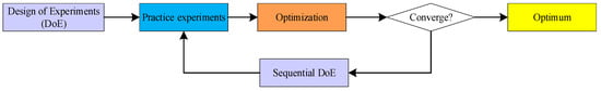
Figure 1.
Framework of ordinary experiment optimization.
In instances where experimental costs are excessively high, the establishment of experimental environments is challenging, or labor expenditures associated with experimentation are substantial, simulation experiments grounded in computational analysis represent a feasible alternative. These simulation experiments, referred to as multi-fidelity experiments, are conducted across various scales. Optimization processes relying on multi-fidelity experiments can be effectively implemented through multi-fidelity surrogate models. The overall procedure is primarily divided into four essential phases: initial DoE, implementation of multi-fidelity experiments, surrogate-based optimization, and sequential DoE. This experimental framework is depicted in Figure 2. In the inner loop of the surrogate optimization algorithm, several key components play a crucial role in enhancing the efficiency of surrogate-based experimental optimization. These components include the selection and allocation of initial samples, the development of the surrogate model, and the formulation of criteria for optimization. Each of these elements plays a significant role in enhancing the overall performance of the optimization process.
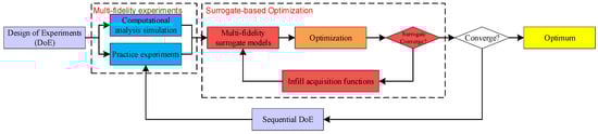
Figure 2.
Framework of multi-fidelity surrogate-based experiment optimization.
2.2. Initial Sample Experiments
In the context of both classical and surrogate-based experimental design optimization, the initial sampling phase is of paramount importance. Unlike gradient-based optimization, where the initial sample primarily serves as a starting point, it is essential to ensure that this sample also contributes to effective space filling.
Assume that the true model of a system in region is
where is the factor and is the response. It is commonly recognized that the experimental sample space is represented as a hypercube, designated as . For the purpose of consistency and simplicity, this space is typically defined as the unit cube, referred to as . Let represent the set of design points on . The objective of the experimental design is to develop a surrogate model through the implementation of design .
To estimate the true model presented in Equation (1), it is customary to derive an estimate of parameter
by utilizing the sample mean.
The Monte Carlo method is recognized as one of the most straightforward random sampling techniques. In this methodology, signifies samples taken from a uniform distribution within a defined set . The estimated variance is referred to as . In accordance with the central limit theorem, it is possible to compute the 95% confidence interval for the variance, which assesses the relationship between the sample mean and the overall mean.
In numerous instances, the variance in estimation caused by random sampling can be excessively large. Latin hypercube sampling (LHS), introduced by McKay [32], is a popular method used to minimize this estimation variance. This technique involves dividing the test area into layers based on variable , ensuring that each layer maintains the same marginal probability . After this division, a sample is taken from each layer.
When a prior distribution is available, Latin hypercube sampling (LHS) may be conducted according to the specified form of the prior, as elaborated in Appendix A. Figure 3 illustrates an LHS design that utilizes a two-dimensional normal distribution as its prior.
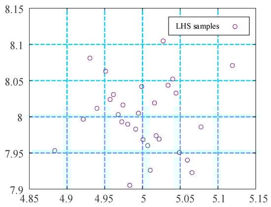
Figure 3.
Latin hypercube sampling of normal distribution.
2.3. Multi-Fidelity Hamilton Kriging Model
The primary distinction of the Kriging model, in contrast to other models, is its foundation as a non-parametric regression model. Originating from the field of geo-statistics, Kriging posits that a correlation exists between any two exploration points within a specific area, with this correlation being solely dependent on the distance separating them. In the context of a two-dimensional plane, it is assumed that this correlation is pervasive and follows a random stationary distribution. This stationary distribution is termed the correlation function. The strength of the correlation between two known samples is quantified by the correlation coefficient. When a sufficient number of samples are available, it becomes feasible to establish a regression model based on the correlation function, wherein the parameters of the correlation function can be estimated using the maximum likelihood method. For additional details, please refer to Appendix B.
Considering the m-dimensional problem, a small amount of expensive but accurate data (high-fidelity, HF) is established as , and a large amount of cheap but low-precision data (low-fidelity, LF) is established as .
where is the HF input set and is the HF response value set. Similarly, is considered the sampled set of LF data.
The multi-fidelity Hamiltonian Kriging (MHK) can be constructed as follows:
where is an adaptive parameter of gradient Kriging and is a scale parameter. The value of can be obtained as
where the ith column of is defined as the column that has an equal value in all rows at , and is defined as the column that has an equal value in .
The selection of MHK is predicated on the capability of the HMC process to effectively simulate the multi-fidelity Kriging target, thereby facilitating faster evaluations. Furthermore, the HMC method’s proficiency in traversing and remaining within the typical distribution permits sampling from the low-fidelity data set , while also enabling adaptive access to the high-fidelity data set for the acquisition of new samples.
2.4. Sequential Infill Sampling Strategy
Following the development of a surrogate model utilizing existing sample points, it may be employed to predict the response for any sample point within the designated sample space. However, should the surrogate model fail to meet the requisite accuracy standards, it is essential to manually introduce additional sample points and modify the parameters to enhance accuracy. In general, the optimization of the surrogate model’s accuracy primarily emphasizes global optimization strategies.
The parameter serves as a tuning variable that establishes a balance between absolute error and prediction variance. When denotes the new sample, it corresponds to the widely recognized strategies of EI or PI, as detailed in Appendix C. In contrast, when signifies the new sample, it aligns with the approach aimed at maximizing the squared predicted error.
2.5. Performance Criteria
Quantifying the error in surrogate models can be classified into two primary methods: (1) methods that require additional data, such as test data sets; (2) methods that rely on existing data. The first method is frequently utilized in machine learning, while the second is more prevalent in statistical science. The root-mean-square error (RMSE) serves as an effective measure of global error within the design domain.
where is the real response of the function and is the predicted response of the surrogate model at . However, the test data set can be costly, so the Cross-Validation (CV) method provides a solution for this circumstance.
where is the number of omitted sample points at the kth iteration of surrogate modeling. As the leave-one-out validation (LOO), the k-fold cross-validation [33] method is an extended version of the CV method, and a Predictive Estimation of Model Fidelity (PEMF) is an even more extended of k-fold CV, which can be found in [34].
3. Adaptive Sequential Infill Sampling Strategy for MHK
3.1. Definition of Multi-Fidelity Infill Sampling Strategy
In order to propose an efficient infill sampling strategy for the multi-fidelity surrogate model, we first formulate a definition of the regular multi-fidelity infill sampling strategy.
For a surrogate model as proposed by Equation (10), the prediction of a multi-fidelity model can be written as
where is a weight parameter that can be solved by the Lagrange multiplier approach from an information economic function from MHK via Cholesky decomposition.
The objective of the infill sampling strategy is to choose an appropriate sample point in the design space to promote the accuracy of the surrogate model sequentially. In the process of MHK modeling, a series prediction can be solved and we get
The multi-fidelity model prediction can be formulated as
Inspired by the EI strategy, Zheng [28] introduced a VFEI strategy specifically designed for multi-fidelity infill sampling. The choice to incorporate LF samples or HF samples is determined by the sequential order of the pairs .
3.2. Probabilistic Nearest Neighborhood
Probabilistic Nearest Neighborhood (PNN) was initially introduced by Holmes as a method for pattern classification within the field of statistical computation. As an advancement to K-Nearest Neighbor (KNN) classification, PNN offers a probabilistic framework that effectively addresses the uncertainty associated with interactions between neighborhoods. This methodology yields a continuous marginal probability prediction distribution within the interval (0,1). The primary advantage of PNN is its ability to provide a predictive distribution for new observations, resulting in a smoother representation of neighborhoods that extend into regions characterized by sparse data. To enhance the effective utilization of the expected improvement information derived from newly added sample points, it is advisable to employ PNN to deliver the predictive distribution for pre-added samples across various fidelity models. This approach will facilitate informed decision making concerning the addition of multi-fidelity samples.
Consider a set of responses of with observations.
where is the training set and is the test set. Both of them are matrices of , is an vector of known class labels for the training data set, and is an vector of unknown class labels that needs to be recognized.
where is the Dirac function, is an interaction parameter between the neighborhoods of and , k is the neighborhood size of a KNN classifier of Q classes, and calculates the proportion of training points in the k nearest neighborhoods of of class q. And a new point predictive distribution can be calculated as
An example illustrating the contrast between PNN, KNN, and Discriminant Adaptive Nearest Neighbor (DANN) is shown in Figure 4 and Figure 5 using a set of sine wave-shaped decision boundaries.
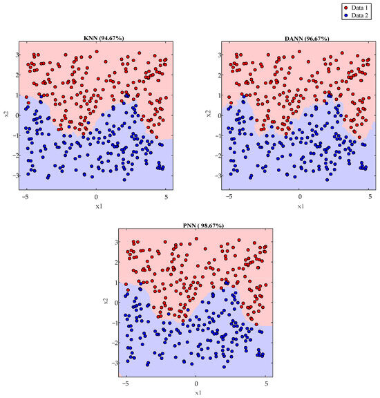
Figure 4.
Pattern classification of sine wave-shaped boundary data sets via KNN, DANN, and PNMN.
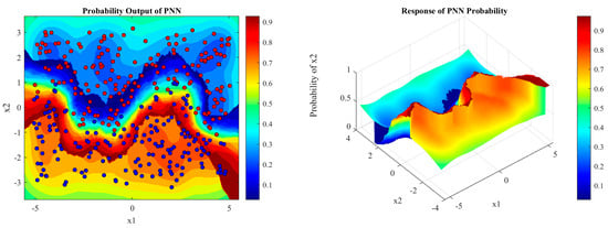
Figure 5.
PNN probability distribution of sine wave-shaped boundary data sets.
3.3. Adaptive Sequential Infill Sampling Strategy
Inspired by the principles of PNN, this paper presents a novel framework for the multi-fidelity addition criterion utilized in MHK. We employ Bayesian inference to determine the optimal number of samples to be incorporated at each fidelity level. Furthermore, we apply PNN to evaluate the neighborhood of the newly added points. The neighborhood points for each fidelity level are ranked according to their mean values, with the highest-scoring points being designated as infill samples for subsequent trials.
Theorem 1.
Bayes formula
- Let represent a partition of the sample space . For any event A, it follows that
Theorem 2.
Bayesian Prediction
- Assume for , and ; then, the prediction of the posterior predictive distribution can be calculated asWith the prediction of MHK as (10), we can calculate the predictive distribution of any fidelity:And with the help of (24),The predictive distribution of any infill sample can be expressed asBy substituting Equations (27) and (28) into Equation (18), it is possible to obtain a similar structural representation:
Note: The posterior probability density function (PDF) of the sequential samples at the ith fidelity level is subtracted from the current minimum multi-fidelity response. This approach serves two primary objectives: it not only considers the posterior response associated with the newly added sample but also ensures that the responses of the “pre-added” samples reflect the mean response within the vicinity, in accordance with the minimum neighborhood parameter estimate of the PNN.
A multi-fidelity infill decision-making framework is established as follows:
It is noted that ASIS contributes to the improvement in the MF model. In addition, means that to calculate any potential improvement for the MF model, after calculation of all infill samples for the MF model, a Bayesian predictor for is added, and then
Figure 6 presents the optimization structure delineated in this paper, which is primarily categorized into three components: the initial design of experiments (DoE), the multi-fidelity surrogate model, and infill sample optimization. The Initial DoE involves sampling experiments at varying fidelity levels, utilizing Latin hypercube sampling (LHS). The multi-fidelity surrogate model incorporates the MHK model and employs Predictive Estimation of Model Fidelity (PEMF) for root-mean-square error (RMSE) cross-validation, thereby enhancing the accuracy of the model. Additionally, the Adaptive Sequential Infill Sampling (ASIS) strategy proposed in this paper is utilized for effective discrimination among multi-fidelity points.
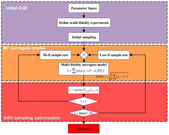
Figure 6.
Framework of ASIS strategy.
4. Results and Discussion
In this section, two numerical simulations and one engineering example are used to demonstrate the proposed method.
4.1. Forrestal Function
In this one-dimensional test, Forrestal functions are employed to demonstrate the proposed ASIS strategy. The constants A, B, and C can be adjusted to enhance the accuracy of the low-fidelity function.
where , , is a high-fidelity model, and is a low-fidelity model. And there is an optimal solution at with the value of .
In this test simulation, we first use 10 low-fi samples at and 4 hi-fi samples at to build the initial surrogate model by MHK, which can be found in Figure 7.
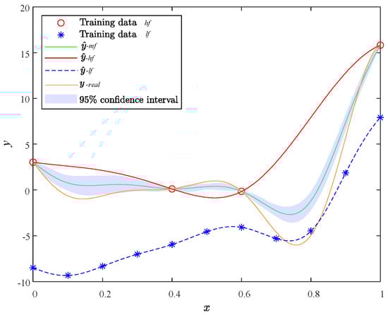
Figure 7.
Initial surrogate model by MHK.
The infill process of the MHK surrogate model using the ASIS method is illustrated in Figure 8, Figure 9, Figure 10 and Figure 11. Each figure consists of two components: the surrogate functions and the ASIS criterion. During each iteration, the ASIS compares the optimal neighborhood improvement achieved with high-fidelity and low-fidelity samples. It then selects the median of the PNN to add a new sample. The accuracy of each model is assessed using the RMSE of the PEMF. If the accuracy does not meet the set requirement (defined here as 0.01), additional samples are incorporated to update the surrogate model. Throughout the process of four sample additions, two high-fidelity samples (, ) and two low-fidelity samples (, ) are added.
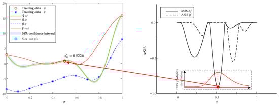
Figure 8.
Optimization iteration 1 of Forrestal function via MHK and ASIS.
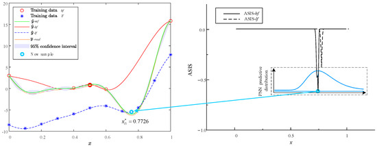
Figure 9.
Optimization iteration 2 of Forrestal function via MHK and ASIS.
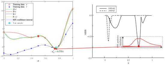
Figure 10.
Optimization iteration 3 of Forrestal function via MHK and ASIS.
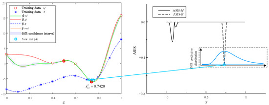
Figure 11.
Optimization iteration 4 of Forrestal function via MHK and ASIS.
To further demonstrate the efficacy of the proposed method, the trial iteration limit is established at 10, with a corresponding RMSE convergence value of 0.01. For the purpose of comparison, we employ several methods, including VF-EI, augmented EI, and AMEI, utilizing the surrogate model that was originally proposed with these methods. Additionally, to control for variables, we incorporate the MHK surrogate model utilized in this paper for a comprehensive comparative analysis. The results of contemporary surrogate models employing various infill sampling strategies are delineated in Table 1. The median error predictive distribution of RMSE via PEMF is shown in Figure 12. While the optimal value is denoted as , it is observed that both the original EI and the augmented EI methodologies predominantly focus on the incorporation of high-fidelity samples during the sampling process. Conversely, the VF-EI and the AMEI minimize the inclusion of a limited number of high-fidelity samples; however, these approaches still necessitate multiple cycles of sample addition, leading to a significantly high total computational cost. The strategy introduced in this paper, referred to as MHK+ASIS, successfully reduces both the quantity of high-fidelity samples added and the overall number of samples incorporated, while maintaining comparable accuracy.

Table 1.
Results of Forrestal function via modern surrogate models and infill strategies.
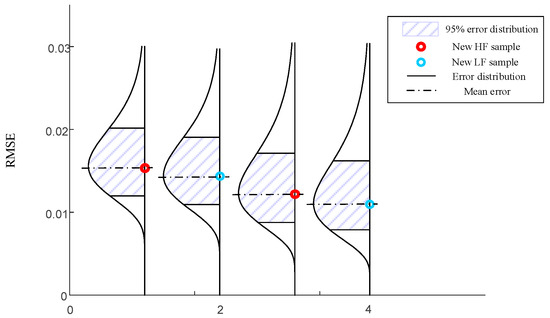
Figure 12.
Median error predictive distribution of RMSE via PEMF.
4.2. Rosebrock Function
A widely recognized 2D optimization function serves as the basis for demonstrating the proposed ASIS. The definitions of the multi-fidelity functions are presented as follows:
where , is the high-fidelity version, and the low-fidelity versions are parameterized by [35]. The cost ratio (CR) for each fidelity by is settled as Table 2. The four types fidelity of Kriging surrogate models optimization via GA are shown in Figure 13.
Table 2.
Parameters of multi-fidelity Rosebrock function.
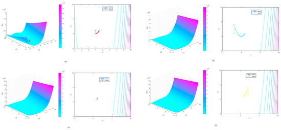
Figure 13.
Surrogate model with four fidelity Rosebrock optimizations via GA.
Initially, each surrogate model was formulated based on a single fidelity function. The sampling for each model was conducted in accordance with the CR, utilizing 40, 40,000, 400, and 4000 initial sample points ranging from high to low fidelity to establish the initial Kriging model. The Genetic Algorithm (GA) was employed for optimization, with a specified convergence accuracy of 0.01. Table 3 outlines the number of iterations and the maximum absolute error (MAE) associated with the convergence of each model.
Table 3.
Optimization results of different fidelity surrogate models.
A high-fidelity surrogate model demonstrates the ability to achieve a satisfactory level of accuracy with a minimal number of iterations. In contrast, a low-fidelity surrogate model, constructed from a substantial number of samples, may attain commendable accuracy; however, it remains inferior to the high-fidelity counterpart. Furthermore, the implementation of a surrogate model that leverages a large sample size can effectively decrease the number of convergence iterations required for optimization using GA. To enhance our analysis, we developed a multi-fidelity MHK surrogate model utilizing the available test samples. Employing the sequential optimization of ASIS, we initially conducted an experiment focused on sample augmentation. Following the attainment of a surrogate model with a relatively high level of accuracy (PEMF = 0.01), we proceeded to execute further optimization, yielding the subsequent results:
The surrogate model based on the MHK was enhanced through the optimization framework outlined in the article, allowing for the incorporation of samples with varying levels of fidelity, shown in Figure 14. The red boxes indicate the new high-fidelity samples (i = 1) introduced by the ASIS method, while the blue boxes denote the collection of low-fidelity samples (i = 2, 3, 4) added. Following the addition of a limited number of high-fidelity samples (i = 14) and low-fidelity samples (i = 95), the PEMF of MHK achieved the stipulated requirement of 0.01. Optimization history of HF and MF surrogate model is shown in Figure 15.
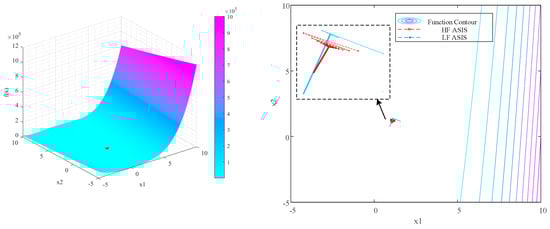
Figure 14.
Rosebrock MHK model via ASIS.
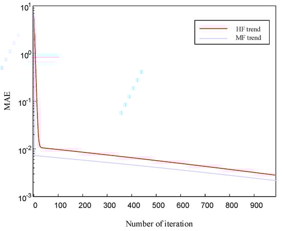
Figure 15.
Optimization iterations of HF and MF surrogate model.
An analysis is conducted to compare the performance of modern surrogate models that utilize various infilling sampling strategies. Results of the comparison are detailed in Table 4. The standard Rosebrock function features an extreme point, denoted as , located at (1, 1). However, as the low-fidelity CR scale varies, this extreme point also shifts accordingly. We established the maximum number of infilling iterations at 30 and repeated the experiment 10 times for each strategy to ensure the robustness of the findings. The average error for each experiment is expressed as the root-mean-square error (RMSE). The data indicate that the results for the HK+AMEI, MHK+AMEI, and MHK+ASIS strategies exhibit relative stability and accuracy. Significantly, the MHK+ASIS method proposed in this study minimizes the requirement for additional high-fidelity samples while concurrently reducing the mean error, thereby providing an efficient solution for experimental optimization.
Table 4.
Results of Rosebrock function via modern surrogate models and infill strategies.
4.3. Naca 0012 Airfoil Validation
The initial application within the field of aerospace engineering pertains to the optimization of a 2D NACA 0012 wing, specifically aimed at determining its optimal lift-to-drag ratio. For the purpose of multi-fidelity validation, a mesh grid family has been supplied by the Langley Research Center [36], as illustrated in Figure 16. Both mesh families share the same leading edge, and the analysis of the airfoil is conducted under conditions characterized by a Mach number of 0.15 and a Reynolds number of 6 million, facilitating free transition. For the validation of experimental results, wind tunnel test data from Ladson is utilized as high-fidelity validation data.
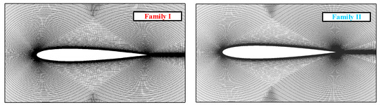
Figure 16.
Multi-fidelity grid for NACA 0012 wing optimization.
First, the simulation is performed on Xflow, 4 angles of attack (AoAs) are sampled from the Family 2 grid for HF data, and 16 AoAs are sampled from the Family 1 grid for LF data. With the initial LHS data sets, an MHK is built first as shown in Figure 17.
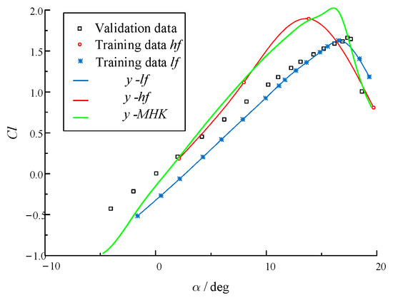
Figure 17.
MHK model with initial NACA Xflow data.
The objective of this multi-fidelity surrogate model is to identify the maximum lift ratio of the NACA 0012 airfoil. Historically, conducting wind tunnel experiments has been a costly endeavor, often succeeded by high-precision large eddy simulations (CFDs). This study utilizes the infill strategy detailed in this paper to incorporate additional samples, comparing its effectiveness with the widely used VFEI and augmented EI strategies. In summary, the proposed ASIS, which integrates three samples (two lf samples and one hf sample), demonstrates a performance that is comparable to the VFEI approach, which adds three samples (one lf sample and two hf samples). Conversely, the augmented EI strategy enhances accuracy by incorporating three hf samples.
The MHK infill sample optimizations via ASIS, VFEI, and augmented EI are shown in Figure 18. A thorough analysis indicates that while the augmented EI method improves overall accuracy and aligns closely with the high-fidelity model, it does neglect the trend information available from low-fidelity samples. The VFEI approach, leveraging a comparative strategy for each added sample, tends to favor high-fidelity samples in the pursuit of improved accuracy. In contrast, the strategy presented in this paper considers the potential probabilistic neighborhood of the added samples, effectively balancing the immediate accuracy enhancements provided by high-fidelity samples with the trend (gradient) improvements that low-fidelity sample points contribute.
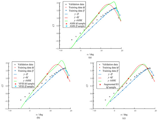
Figure 18.
MHK infill sample optimizations via ASIS, VFEI, and augmented EI.
Furthermore, the proposed ASIS enables PEMF error prediction to achieve an RMSE accuracy of less than 0.005 after the addition of only eight sample points, which is shown in Figure 19. This finding suggests that, prior to conducting actual tests, the integration of a limited number of samples through ASIS facilitates a progressive prediction of PEMF. Consequently, this method allows for the determination of the optimal number of samples required to attain the desired accuracy, thus minimizing the costs associated with trial and error.
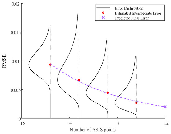
Figure 19.
NACA 0012 median error predictive distribution of RMSE via PEMF.
5. Conclusions
In this article, the Adaptive Sequential Infill Sampling (ASIS) strategy was introduced, which significantly enhances the accuracy and efficiency of sample addition experiments in multi-fidelity surrogate modeling, particularly for Multi-fidelity Hamilton Kriging. The ASIS method was validated using two numerical simulations and was applied to a flow optimization analysis problem involving a NACA 0012 airfoil. The conclusions drawn from this study are as follows.
- (1)
- The Adaptive Sequential Infill Sampling strategy is an advancement of the Best Neighborhood-based Kriging infill method, specifically designed for the optimization of multi-fidelity experiments. This strategy effectively balances accuracy and efficiency in sequential experimental optimization by employing a Probabilistic Neural Network (PNN)-enhanced expected improvement (EI) methodology. Both numerical analyses and practical applications demonstrate the effectiveness of the proposed approach.
- (2)
- The Adaptive Sequential Infill Sampling strategy is an infill strategy that is used for experimental optimization error prediction. In order to balance the exploration between multi-fidelity models, a Probability Nearest Neighborhood method is used not only for error distribution prediction, but also for criteria optimization. Consequently, the ASIS framework delivers a robust estimate of errors throughout the sequential optimization process.
- (3)
- The Adaptive Sequential Infill Sampling strategy demonstrates greater utility and cost-effectiveness for multi-fidelity sequential infill sampling compared to certain advanced infill strategies. This is primarily due to its capability to compute posterior predictive distributions, which enhances the estimation of sampling errors in neighboring samples. Moreover, the application of PNN for predictions based on specified error sampling enables the utilization of fewer high-fidelity data points while still meeting the required root-mean-square error (RMSE) criteria.
In addition to the airfoil optimization engineering problem discussed earlier, the ASIS framework is fully capable of addressing a wide range of sequential optimization challenges that necessitate the incorporation of new samples. In future applications, ASIS has the potential to enhance its predictive capabilities in sequential experimental design by leveraging additional Bayesian frameworks.
Author Contributions
The methodology of Adaptive Sequential Infill Sampling strategy was proposed by S.Z.; S.Z. wrote the majority of the manuscript text and conducted the numerical and engineering validation; J.M. reviewed and edited the manuscript. All authors have read and agreed to the published version of the manuscript.
Funding
This research received no external funding.
Data Availability Statement
Data will be made available on reasonable request.
Conflicts of Interest
The authors declare no conflicts of interest.
Appendix A
Let the experimental area be represented as , while signifies the uniform design , in which each column of is a permutation of . The Latin hypercube design entails conducting random sampling within .
Let denote a Latin hypercube design, wherein each subcube, represented as , possesses a side length of and is centered at , referred to as . Additionally, let be a random sample sourced from . The resulting set, designated as , is recognized as Latin hypercube sampling.
Appendix B
The Kriging model is defined as a multivariate polynomial, namely
where for , we can set as a basis function and as the coefficient. Then, a Kriging model based on the sampled data set can be built:
After building Kriging, the Kriging predictor for any unsampled site can be obtained as
where for the regression function, we have an matrix F as
And the correlation matrix is defined by n × n matrices :
where is built up with a set of , which can be identified in Appendix A. After the fitting process, the prediction variance at any untried sample can be computed as
where for the unsampled point , we have as a model prediction matrix, as a coefficient vector, as a coefficient matrix between and , and as a process variance vector.
Appendix C
The Expectation Improvement (EI) algorithm is often called an efficient global optimization algorithm (EGO). Here, it is necessary to assume that the current optimal objective function value is , and the predicted response from Kriging follows .
which can be explored as
Then, the improvement of the objective function is set as
The EI function is derived by weighting potential improvements with probability densities and expressed as
where is the normal density and is the distribution function, and new points can be added as the EI function reaches its highest value.
The Probability Improvement (PI) algorithm is similar to the Expectation Improvement algorithm, and new samples can be added when the probability of the target function reaches its maximum. The Probability Improvement function is written as
where it is assumed that the random variable follows a normal distribution when setting .
With the help of a reparameterization trick and (A7), the improvement function (A9) can be rewritten as
Therefore,
where and .
References
- Lei, B.; Kirk, T.Q.; Bhattacharya, A.; Pati, D.; Qian, X.; Arroyave, R.; Mallick, B.K. Bayesian optimization with adaptive surrogate models for automated experimental design. npj Comput. Mater. 2021, 7, 194. [Google Scholar] [CrossRef]
- Samadian, D.; Muhit, I.B.; Dawood, N. Application of Data-Driven Surrogate Models in Structural Engineering: A Literature Review. Arch. Comput. Methods Eng. 2025, 32, 735–784. [Google Scholar] [CrossRef]
- Zanobini, A.; Sereni, B.; Catelani, M.; Ciani, L. Repeatability and Reproducibility techniques for the analysis of measurement systems. Measurement 2016, 86, 125–132. [Google Scholar] [CrossRef]
- Kuhn, D.R.; Reilly, M.J. An investigation of the applicability of design of experiments to software testing. In Proceedings of the 27th Annual NASA Goddard/IEEE Software Engineering Workshop, Greenbelt, MD, USA, 5–6 December 2002; pp. 91–95. [Google Scholar]
- Fang, K.-T.; Lin, D.K.J.; Winker, P.; Zhang, Y. Uniform Design: Theory and Application. Technometrics 2000, 42, 237–248. [Google Scholar] [CrossRef]
- Park, J.-S. Optimal Latin-hypercube designs for computer experiments. J. Stat. Plan. Inference 1994, 39, 95–111. [Google Scholar] [CrossRef]
- Davis, S.E.; Cremaschi, S.; Eden, M.R. Efficient Surrogate Model Development: Impact of Sample Size and Underlying Model Dimensions. In Computer Aided Chemical Engineering; Eden, M.R., Ierapetritou, M.G., Towler, G.P., Eds.; Elsevier: Amsterdam, The Netherlands, 2018; pp. 979–984. [Google Scholar]
- Fernandez-Godino, M.G.; Haftka, R.T.; Balachandar, S.; Gogu, C.; Bartoli, N.; Dubreuil, S. Noise Filtering and Uncertainty Quantification in Surrogate based Optimization. In Proceedings of the 2018 AIAA Non-Deterministic Approaches Conference, Kissimmee, FL, USA, 8–12 January 2018; American Institute of Aeronautics and Astronautics: Reston, VA, USA, 2018. [Google Scholar] [CrossRef]
- Cheng, K.; Lu, Z.; Ling, C.; Zhou, S. Surrogate-assisted global sensitivity analysis: An overview. Struct. Multidiscip. Optim. 2020, 61, 1187–1213. [Google Scholar] [CrossRef]
- Myers, R.H.; Montgomery, D.C. Response Surface Methodology. IIE Trans. 1996, 28, 1031–1032. [Google Scholar] [CrossRef]
- Xiu, D.; Karniadakis, G.E. Modeling uncertainty in flow simulations via generalized polynomial chaos. J. Comput. Phys. 2003, 187, 137–167. [Google Scholar] [CrossRef]
- Krige, D.G. A statistical approach to some basic mine valuation problems on the Witwatersrand. J. S. Afr. Inst. Min. Metall. 1951, 52, 119–139. [Google Scholar]
- Regis, R.G.; Shoemaker, C.A. Constrained Global Optimization of Expensive Black Box Functions Using Radial Basis Functions. J. Glob. Optim. 2005, 31, 153–171. [Google Scholar] [CrossRef]
- Mangasarian, O.L.; Musicant, D.R. Robust linear and support vector regression. IEEE Trans. Pattern Anal. Mach. Intell. 2000, 22, 950–955. [Google Scholar] [CrossRef]
- Weinmeister, J.; Gao, X.; Roy, S. Analysis of a Polynomial Chaos-Kriging Metamodel for Uncertainty Quantification in Aerodynamics. AIAA J. 2019, 57, 2280–2296. [Google Scholar] [CrossRef]
- Dwight, R.; Han, Z.-H. Efficient Uncertainty Quantification Using Gradient-Enhanced Kriging. In Proceedings of the 50th AIAA/ASME/ASCE/AHS/ASC Structures, Structural Dynamics, and Materials Conference, Palm Springs, CA, USA, 4–7 May 2009; American Institute of Aeronautics and Astronautics: Reston, VA, USA, 2009. [Google Scholar] [CrossRef]
- Han, Z.; Zimmermann, R.; Goertz, S. On improving Efficiency and Accuracy of Variable-Fidelity Surrogate Modeling in Aero-data for Loads Context. In Proceedings of the European Air and Space Conference, Manchester, UK, 26–29 October 2009; Royal Aeronautical Society: London, UK, 2009. [Google Scholar]
- Kennedy, M.C.; O’Hagan, A. Predicting the output from a complex computer code when fast approximations are available. Biometrika 2000, 87, 1–13. [Google Scholar] [CrossRef]
- Forrester, A.I.J.; Sóbester, A.; Keane, A.J. Multi-fidelity optimization via surrogate modelling. Proc. R. Soc. A Math. Phys. Eng. Sci. 2007, 463, 3251–3269. [Google Scholar] [CrossRef]
- Han, Z.-H.; Görtz, S. Hierarchical Kriging Model for Variable-Fidelity Surrogate Modeling. AIAA J. 2012, 50, 1885–1896. [Google Scholar] [CrossRef]
- Han, Z.-H.; Görtz, S.; Zimmermann, R. Improving variable-fidelity surrogate modeling via gradient-enhanced kriging and a generalized hybrid bridge function. Aerosp. Sci. Technol. 2013, 25, 177–189. [Google Scholar] [CrossRef]
- Zhang, S.; Ma, J. Applied Hamiltonian Monte Carlo for multi-fidelity kriging modelling in experiment optimization. Eng. Optim. 2025, 1–33. [Google Scholar] [CrossRef]
- Wilson, J.; Hutter, F.; Deisenroth, M. Maximizing acquisition functions for Bayesian optimization. In Proceedings of the Thirty-Second Annual Conference on Neural Information Processing Systems (NIPS), San Diego, CA, USA, 2–8 December 2018. [Google Scholar]
- Kushner, H.J. A New Method of Locating the Maximum Point of an Arbitrary Multipeak Curve in the Presence of Noise. J. Basic Eng. 1964, 86, 97–106. [Google Scholar] [CrossRef]
- Ghoreyshi, M.; Badcock, K.J.; Woodgate, M.A. Accelerating the Numerical Generation of Aerodynamic Models for Flight Simulation. J. Aircr. 2009, 46, 972–980. [Google Scholar] [CrossRef]
- Hertz-Picciotto, I.; Rockhill, B. Validity and Efficiency of Approximation Methods for Tied Survival Times in Cox Regression. Biometrics 1997, 53, 1151–1156. [Google Scholar] [CrossRef]
- Currin, C.; Mitchell, T.; Morris, M.; Ylvisaker, D. Bayesian Prediction of Deterministic Functions, with Applications to the Design and Analysis of Computer Experiments. J. Am. Stat. Assoc. 1991, 86, 953–963. [Google Scholar] [CrossRef]
- Zhang, Y.; Han, Z.-H.; Zhang, K.-S. Variable-fidelity expected improvement method for efficient global optimization of expensive functions. Struct. Multidiscip. Optim. 2018, 58, 1431–1451. [Google Scholar] [CrossRef]
- Hao, P.; Feng, S.; Li, Y.; Wang, B.; Chen, H. Adaptive infill sampling criterion for multi-fidelity gradient-enhanced kriging model. Struct. Multidiscip. Optim. 2020, 62, 353–373. [Google Scholar] [CrossRef]
- Dong, H.; Sun, S.; Song, B.; Wang, P. Multi-surrogate-based global optimization using a score-based infill criterion. Struct. Multidiscip. Optim. 2019, 59, 485–506. [Google Scholar] [CrossRef]
- Zhang, S.; Ma, J. Kriging-based design of sequential experiment via best neighborhoods for small sample optimization. In Proceedings of the 43rd Chinese Control Conference (CCC), Kunming, China, 28–31 July 2024; pp. 7006–7011. [Google Scholar]
- McKay, M.D.; Bolstad, J.W.; Whiteman, D.E. Application of Statistical Techniques to the Analysis of Reactor Safety Codes; Los Alamos National Laboratory (LANL): Los Alamos, NM, USA, 1978; p. 31. [Google Scholar]
- Fushiki, T. Estimation of prediction error by using K-fold cross-validation. Stat. Comput. 2011, 21, 137–146. [Google Scholar] [CrossRef]
- Mehmani, A.; Chowdhury, S.; Messac, A. Predictive quantification of surrogate model fidelity based on modal variations with sample density. Struct. Multidiscip. Optim. 2015, 52, 353–373. [Google Scholar] [CrossRef]
- Olivanti, R.; Gallard, F.; Brézillon, J.; Gourdain, N. Comparison of Generic Multi-Fidelity Approaches for Bound-Constrained Nonlinear Optimization Applied to Adjoint-Based CFD Applications. In Proceedings of the AIAA Aviation 2019 Forum, Dallas, TX, USA, 17–21 June 2019; American Institute of Aeronautics and Astronautics: Reston, VA, USA, 2019. [Google Scholar] [CrossRef]
- Ladson, C.L. Effects of Independent Variation of Mach and Reynolds Numbers on the Low-Speed Aerodynamic Characteristics of the NACA 0012 Airfoil Section; National Aeronautics and Space Administration: Washington, DC, USA, 1988.
Disclaimer/Publisher’s Note: The statements, opinions and data contained in all publications are solely those of the individual author(s) and contributor(s) and not of MDPI and/or the editor(s). MDPI and/or the editor(s) disclaim responsibility for any injury to people or property resulting from any ideas, methods, instructions or products referred to in the content. |
© 2025 by the authors. Licensee MDPI, Basel, Switzerland. This article is an open access article distributed under the terms and conditions of the Creative Commons Attribution (CC BY) license (https://creativecommons.org/licenses/by/4.0/).