Research on Optimization Technology of Minimum Specific Fuel Consumption for Triple-Bypass Variable Cycle Engine

Abstract

This paper investigates the best control method of the lowest specific fuel consumption (SFC) to reduce the specific fuel consumption of the triple-bypass variable cycle engine. Specific fuel consumption is the ratio of fuel flow to thrust. First, the Kriging model of the engine near the supersonic cruise and subsonic cruise state points was extracted using the component-level model of the triple-bypass variable cycle engine, and the PSM was obtained close to the steady-state point. The contribution of each control variable to the engine’s specific fuel consumption was computed using the PSM and, at the same time, due to the linear characteristics of the PSM, it was easy to deal with various constrained linear optimization problems, and the steady-state points with the smallest specific fuel consumption under the constraints could be obtained through the linear optimization algorithm; however, the surge margin and pre-turbine temperature of the optimized point were limited in the optimization process, the method of direct switching inevitably brought the problem of overshoot of the controlled quantity, and the actual controlled quantity could still exceed the safe operation boundary of the engine in the process of change. Moreover, the performance optimization control itself is premised on sacrificing the surge margin of the engine, and its operating boundary is closer to the surge line, so the limitation protection problem in the transition state cannot be ignored in the process of performance optimization control. In this paper, a multivariable steady-state controller was designed based on Model Predictive Control (MPC) to meet the needs of engine optimization control mode switching. The simulation results of the supersonic cruise mode show that the minimum fuel consumption control can reduce the fuel consumption of the engine by 2.6% while the thrust remains constant.

1. Introduction

With the development of the full-authority digital electronic control system and the increasing maturity of multivariable control, performance optimization control (PSC) was listed as one of the advanced control technologies of aero-engines by the United States National Aeronautics and Space Administration in the 1980s, with the aim of improving/optimizing the quasi-steady-state performance of aircraft and propulsion systems. The mission profile analysis of the aero-engine shows that it spends most of its time cruising [1,2,3,4,5]. In order to achieve the purpose of saving fuel, increasing economy, and increasing the range of the aircraft, it is necessary to explore the minimum specific fuel consumption mode of the engine during the cruising phase [5,6].

The engine studied in this paper is a new triple-bypass variable cycle engine proposed by the Gas Turbine Basic Science Center [7,8]. This configuration requires the engine to meet the requirements of a low-speed subsonic cruise mode economy, medium supersonic flight mode economy and acceleration, and high-speed mode continuous high thrust in airspace, a speed range, and for this purpose, the design ideas of a high flow rate, high throttle ratio, and a high turbine front temperature in the full speed range are proposed [9]. The high-flow dual-variable cycle engine has many working modes, including complex and changeable air flow paths, harsh operating conditions, different working states of each combustion chamber in different modes [10], and a large gap in control strategies, so it is necessary to design different control rules according to the specific cruise mode (subsonic cruise, supersonic cruise) [11]. In the high-speed mode, the double-variable combustion chamber and afterburner work at the same time, and the combustion efficiency of the afterburner is required to be far lower than the combustion efficiency of the double-variable combustion chamber; specific fuel consumption also increases sharply and will greatly shorten the combat radius of the aircraft. For this reason, it is necessary to extend the minimum fuel consumption mode to the afterburner state under the premise of ensuring the safe and stable operation of the engine, appropriately sacrifice the engine surge margin, readjust the fuel distribution strategy under the condition that the thrust remains unchanged, give full play to the characteristics of the high combustion efficiency of the double-variable combustion chamber, increase the fuel supply of the double-variable combustion chamber, and reduce the fuel supply of the afterburner so as to achieve the purpose of saving fuel consumption [12]. Therefore, there is an urgent need for a component-level model based on high-precision, high-through-flow dual-variable cycle engines [13,14,15]. We carried out research on the control mechanism of low fuel consumption and breaking through the real-time optimization control technology of the optimal economy (low fuel consumption) of a high-through-flow dual-variable cycle engine [16]. The real-time optimization of specific fuel consumption using PSC technology requires highly accurate and real-time fuel consumption rate prediction algorithms [17].

To this end, this paper first establishes a component-level model, then carries out the research on high-precision airborne composite model technology, and proposes an airborne composite model based on the fusion of the Kriging surrogate model, propulsion system matrix, and state-space equation. Based on the composite model, the linear programming algorithm was used to optimize the minimum specific fuel consumption of the engine in the ground, sub-patrol, and over-patrol conditions [18], and the MPC was used to control the transition state’s great control effect.

2. Research Process

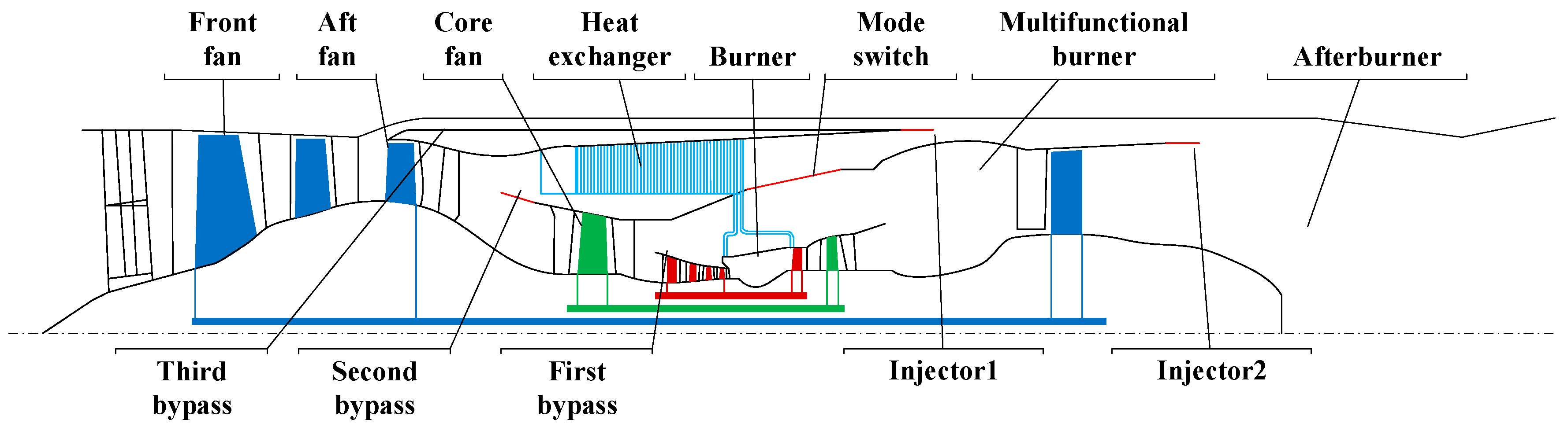
2.1. Overall Structure of Engine

Figure 1 depicts the general layout of the triple-bypass variable cycle engine. Its key parts are the front fan, the aft fan, the core fan, the HPC, the heat exchanger, the burner, the HPT, the IPT, the multifunctional burner, the LPT, the afterburner, and the nozzle. The front and rear fans on the LP rotor are driven by an LPT; the core fan on the IP rotor is powered by the IPT; and the HP rotor is driven by the HPT to drive the HPC. The mode switch is used to control the engine’s back-and-forth motion between the turbofan and jet modes [19,20].

When the mode switch is closed, the engine is in turbofan mode, where the burner and the multifunctional burner can be optionally opened, and the afterburner is closed. The inlet airflow flows through the front fan, partly into the third bypass, and partly into the aft fan, where the airflow again separates into three parts, partly into the second bypass where the heat exchanger is located for heat exchange, partly into the core fan, and finally partly into the LPT for cooling. At the outlet of the HPC, some of the high-temperature gas flows into the heat exchanger duct, where it is cooled by heat exchange with the low-temperature gas from the second bypass and then flows into the HPT. The gas exiting from the IPT is mixed with the gas from the first bypass in the interstage mixer and then flows into the multifunctional burner for re-combustion, passing through the LPT and then completing the final mixing with the gas from the second and third bypass in the mixer and exiting through the tail nozzle to obtain thrust.

When the mode switch is opened, the gas from the second bypass is mixed with the gas from the first bypass and then enters the multifunctional burner; at this time, the burner is closed, the multifunctional burner and the afterburner are opened, the engine is in jet mode, the first bypass and the second bypass are transformed into the inner culvert, and the culvert ratio is reduced, thus ensuring the continuous high-thrust demand of the engine at high speed.

The overall research path is shown in Figure 2. Firstly, the Kriging model is trained by the data of the component model, and the PSM set is obtained by the linearization of the Kriging model. Then, the optimal working point of the engine is obtained by the linear optimization method. Finally, the transition state is controlled by the MPC.

2.2. Establishment of Composite Models

2.2.1. Establishment of the Kriging Model

The Kriging model is the earliest concept of geostatistics; the first law of geography shows that “everything is spatially related, things that are close to each other are more spatially correlated than things that are far away”, which causes a problem. If the value $z_i$ of temperature, air pressure, and humidity of $n$ $m$-dimensional sampling points $x_i$($i=1,2,3,\cdots ,n$) in space is known, it remains to be found how to estimate the value ${\widehat{z}}_p$ of temperature, air pressure, humidity, and other parameters of $x_p$ at any point in space; for this, the Kriging model gives the following interpolation formula.

$${\widehat{z}}_p={\displaystyle \sum _{i=1}^n{\lambda }_i{z}_i}$$

(1)

where ${\lambda }_i$ represents the weight coefficient and its value should be such that the variance between the predicted value ${\widehat{z}}_p$ and the true value $z_p$ is minimized, as follows:

$$\underset{{\lambda }_i}{\min }Var\left({\widehat{z}}_p-z_p\right)$$

(2)

At the same time, the estimated value and the true value need to meet the unbiased estimation conditions:

$$E\left({\widehat{z}}_p\right)=E\left(z_p\right)$$

(3)

The Kriging model assumes that the properties of all points in space are uniform, i.e., for any point in space, as follows:

$$\begin{array}{l}E\left(z_i\right)=c\\ Var\left(z_i\right)={\sigma }^2\end{array}$$

(4)

Then, the above equation turns into solving the optimization problem with constraints.

$$\begin{array}{l}\underset{{\lambda }_i}{\min }{J}_1=Var\left({\widehat{z}}_p-z_p\right)\\ st.{\displaystyle \sum _{i=1}^n{\lambda }_i=1}\end{array}$$

(5)

A common way to solve the above-constrained optimization problem is to use the Lagrange multiplier method, that is, to construct a new objective function, which includes the original constraints, and the solution is the same as the original objective function when the minimum value is obtained:

$$\underset{\varphi ,{\lambda }_i}{\min }{J}_2=Var\left({\widehat{z}}_p-z_p\right)+2\varphi \left({\displaystyle \sum _{i=1}^n{\lambda }_i-1}\right)$$

(6)

The partial derivative for each variable can then be found separately:

$$\left\{\begin{array}{l}{\displaystyle \frac{\partial J_2}{\partial {\lambda }_i}}=0;i=1,2,\cdots n\hfill \\ {\displaystyle \frac{\partial J_2}{\partial \varphi }}=0\hfill \end{array}\right.$$

(7)

The matrix is then converted to form the following:

$$\left[\begin{array}{lllll}{R}_{11}\hfill & R_{12}\hfill & \cdots \hfill & R_{1n}\hfill & 1\hfill \\ R_{21}\hfill & R_{22}\hfill & \cdots \hfill & R_{2n}\hfill & 1\hfill \\ \cdots \hfill & \cdots \hfill & \cdots \hfill & \cdots \hfill & \cdots \hfill \\ R_{n1}\hfill & R_{n2}\hfill & \cdots \hfill & R_{nn}\hfill & 1\hfill \\ 1\hfill & 1\hfill & \cdots \hfill & 1\hfill & 0\hfill \end{array}\right]\left[\begin{array}{l}{\lambda }_1\hfill \\ {\lambda }_2\hfill \\ \cdots \hfill \\ {\lambda }_n\hfill \\ -\varphi \hfill \end{array}\right]=\left[\begin{array}{l}{R}_{1p}\hfill \\ R_{2p}\hfill \\ \cdots \hfill \\ R_{np}\hfill \\ 1\hfill \end{array}\right]$$

(8)

where $R_{ij}$ represents the correlation function between sampling points $x_i$ and $x_j$ and its functional value is only related to distance, which is generally described by the Gaussian kernel function.

$$R_{ij}={\displaystyle \prod _{k=1}^m{e}^{-{\theta }_k{\left|x_{ik}-x_{jk}\right|}^{p_k}}}$$

(9)

where $x_{ik}$ represents the value of the $k$th element in the $i$-th sampling point. ${\theta }_k$ and $p_k$ are the parameters to be determined in the model, and their number depends on the dimension of the sampling point $m$:

$$\begin{array}{l}{\theta }_k=\left[\begin{array}{cccc}{\theta }_1& {\theta }_2& \cdots & {\theta }_m\end{array}\right]\\ p_k=\left[\begin{array}{cccc}{p}_1& p_2& \cdots & p_m\end{array}\right]\end{array}$$

(10)

The Gaussian kernel function is generally a monotonic function of the Euclidean distance between two sample points, and its magnitude reflects the influence of nearby points on the prediction points, and the shorter the distance between the two points, the larger the value of the Gaussian kernel function.

Since $R$ is symmetrically positive, the method of Cholesky decomposition can be used to invert $R$; that is, there is a lower triangular matrix $L$ with all diagonal elements being positive so that the following equation holds.

$$R=L{L}^T$$

(11)

The rule is given as follows:

$$L{L}^T{R}^{-1}=I$$

(12)

Since $L$ is the lower triangular matrix, $L^T{R}^{-1}$ can be quickly solved by the forward push method, and the solution result is $Y$:

$$L^T{R}^{-1}=Y$$

(13)

$L^T$ is the upper triangular matrix, and the above equation can be quickly solved by the algebraic method to obtain the value of $R^{-1}$.

For the engine object of the text study, the input value of the kriging model is the following:

$$x=\left[\begin{array}{lllllll}{W}_{\mathrm{fb}1}\hfill & W_{\mathrm{fb}2}\hfill & {\alpha }_1\hfill & {\alpha }_2\hfill & {\beta }_2\hfill & A_8\hfill & W_{\mathrm{cool}}\hfill \end{array}\right]$$

(14)

The output value is as follows:

$$z=\left[N_{\mathrm{L}}\hspace{1em}{N}_{\mathrm{I}}\hspace{1em}{N}_{\mathrm{H}}\hspace{1em}{F}_{\mathrm{n}}\hspace{1em}{T}_4\hspace{1em}SM{F}_1\hspace{1em}SM{F}_2\hspace{1em}SM{F}_3\hspace{1em}SM{F}_4\hspace{1em}SFC\right]$$

(15)

2.2.2. Propulsion System Matrix Module

The high-flow double-variable cycle engine is a system with strong nonlinearity, and the control of the rest of the input parameters remains unchanged, only changing the fuel flow rate $W_{fb}$ of the main combustion chamber and the area of the tail nozzle throat $A_8$, and the obtained characteristic diagram is shown in Figure 3, and it can be seen that the thrust, $F$, of the engine, the fuel consumption rate, $SFC$, and the surge margin, $SMF$, of the front fan all show nonlinear characteristics.

In order to accurately describe the nonlinear characteristics of the core part of the engine, it is expanded into the form of a propulsion system matrix (PSM) near each steady-state point of the engine. The propulsion matrix is essentially a linearized model with small deviations, and the PSM has good computational accuracy when the engine is not far from the reference point. Compared with the component-level steady-state model, the PSM does not involve complex iterative calculations of aerothermodynamics and rotor dynamics, so the real-time solution performance is greatly improved. At the same time, due to the linear characteristics of the PSM, it is easy to deal with various constrained linear optimization problems, such as the optimization of maximum engine thrust, the optimization of minimum fuel consumption rate, and the optimization of minimum infrared radiation. The PSM has the following general form:

$$\Delta Y=P\Delta X$$

(16)

where $\Delta Y$ is the output change in the system, $\Delta X$ is the input change in the system, and $P$ is the PSM of the system. The PSM of the engine studied in this paper near the steady-state point can be represented by the following:

$$\left[\begin{array}{c}\Delta F\\ \Delta sfc\\ \Delta N_L\\ \Delta N_I\\ \Delta N_H\\ \Delta sm{f}_1\\ \Delta sm{f}_2\\ \Delta sm{f}_3\\ \Delta sm{f}_4\\ \Delta T_4\end{array}\right]=\left[\begin{array}{ccccc}{p}_{1,1}& .& .& .& p_{1,7}\\ .& .& .& .& .\\ .& .& .& .& .\\ .& .& .& .& .\\ p_{10,1}& .& .& .& p_{10,7}\end{array}\right]\left[\begin{array}{c}\Delta W_{fb1}\\ \Delta W_{fb2}\\ \Delta {\alpha }_1\\ \Delta {\alpha }_2\\ \Delta {\beta }_1\\ \Delta {\beta }_2\\ \Delta A_8\end{array}\right]$$

(17)

$N_L$, $N_I$, and $N_H$ denote the low, intermediate, and high-pressure rotor speeds; $sm{f}_1$, $sm{f}_2$, $sm{f}_3$, and $sm{f}_4$ denote the front fan, aft fan, core fan, and low-pressure turbine surge margins; and $p$ is the element of the PSM, which can be calculated by the following equation:

$$p_{i,j}={\displaystyle \frac{\Delta Y_j}{\Delta X_i}}={\displaystyle \frac{Y_j-Y_{j0}}{X_i-X_{i0}}}$$

(18)

where $X_{i0}$ denotes the initial input value, $Y_{j0}$ denotes the initial steady-state point value obtained from the neural network mapping, $X_{i0}$ denotes the input value after a small perturbation occurs, and $Y_{j0}$ denotes the steady-state point value obtained from the neural network mapping after a small perturbation occurs. Because all the parameters in Equation (4) were normalized, which is essentially equivalent to a linear regression model of the engine in a small range, the coefficients in the PSM reflect the degree of influence of the engine’s controllable variables on the output variables, and the contribution is defined as follows:

$$G_{i,j}={\displaystyle \frac{\left|p_{i,j}\right|}{{\displaystyle \sum _{n=1}^7\left|p_{n,j}\right|}}}$$

(19)

2.3. Composite Model Accuracy Verification

Since the linear optimization based on PSM is a form of small-scale optimization near the steady-state point, the dynamic accuracy of the composite model directly affects the optimization results, and then the dynamic accuracy of the composite model can be verified [5].

Taking the over-cruising state as an example, when $Ma=2.35$ and $H=20,000 \mathrm{m}$, the continuous steps of the specific fuel consumption of the combustion chamber, the angle of the turbine guide vane, and the angle of the ducted injector, etc., are shown in Figure 4.

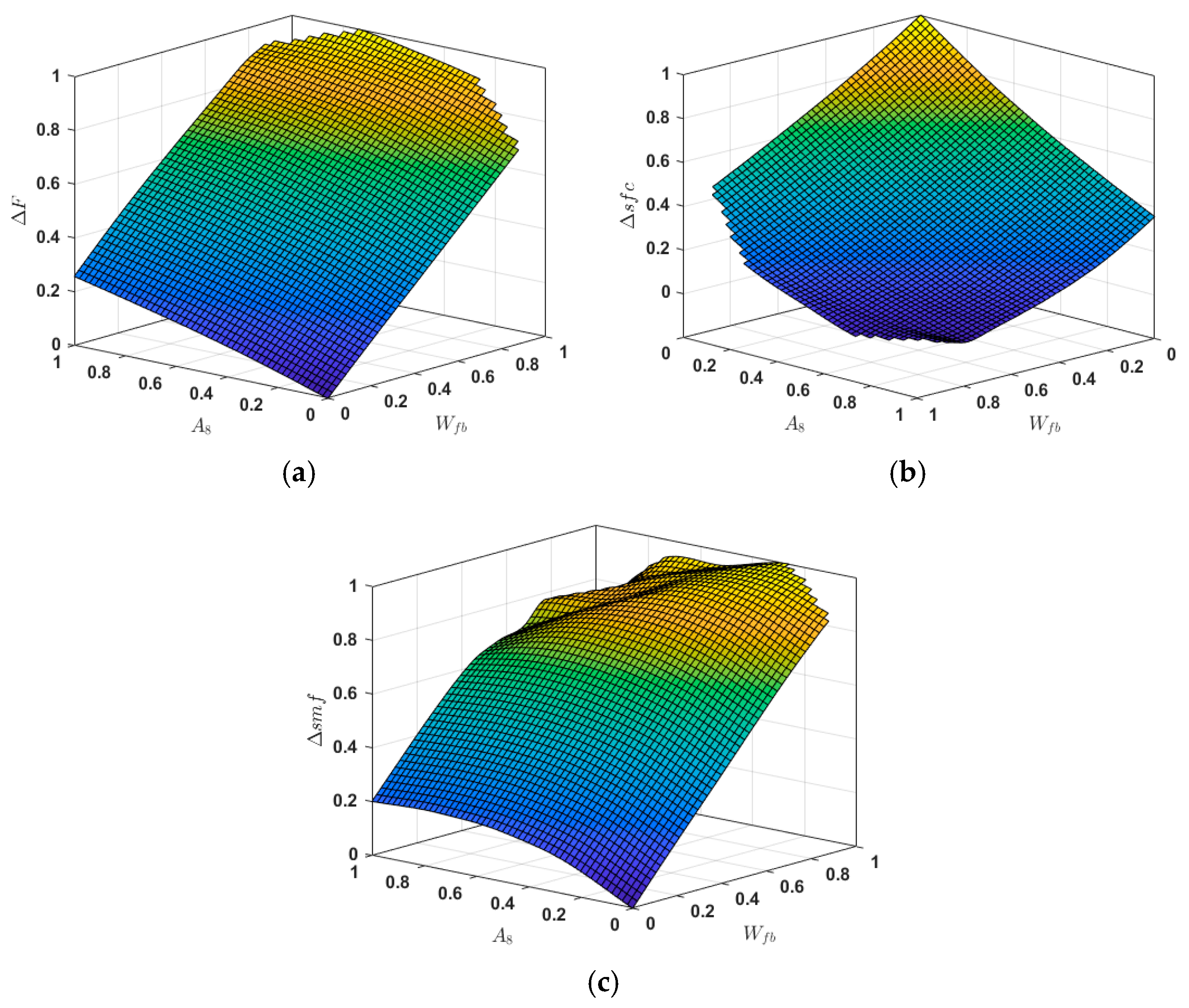
2.4. PSC of Minimum Specific Fuel Consumption

In order to meet the basic performance requirements of the engine, the basic adjustment variables include the fuel flow of the main combustion chamber, the fuel flow of the multifunction combustion chamber, the fuel flow of the afterburner, the angle of the low-pressure turbine guide, the angle of the medium-pressure turbine guide, the area of the tail nozzle throat, the mode switching valve, and the first duct injector and the second duct injector, and the corresponding main functions are given in

Table 1. Engine control quantity.

Variable Name	Variable Meaning
$W_{fb1}$	Fuel flow of burner
$W_{fb2}$	Fuel flow of multifunctional burner
${\alpha }_1$	Guide angle of bypass injector 1
${\alpha }_2$	Guide angle of bypass injector 2
${\beta }_1$	Guide angle of IPT
${\beta }_2$	Guide angle of LPT
$A_8$	Throat area of nozzle

:

Based on the PSM, the aero-engine performance finding problem can be described in the following general form:

$$\begin{array}{ll}\hfill & \min \left(Y_i\right) \mathrm{or} \max \left(Y_i\right)\hfill \\ \hfill \mathrm{s}.\mathrm{t}.& P_{m}X=0\hfill \\ \hfill & P_{n}X\ge 0\hfill \end{array}$$

(20)

where $P_m$ and $P_n$ represent the row vectors of the engine PSM. For the aero-engine minimum SFC model, the optimization objective is $\min \left(\Delta sfc\right)$. It is necessary to ensure that the engine does not over-heat, over-rotate, or surge, and the thrust needs to be constant as follows [6]:

$$\begin{array}{ll}& \min \left(\Delta sfc\right)\\ s.t.& \Delta F=0\\ & \Delta N_{\mathrm{L}\min }\le \Delta N_{\mathrm{L}}\le \Delta N_{\mathrm{L}\max }\\ & \Delta N_{\mathrm{I}\min }\le \Delta N_{\mathrm{I}}\le \Delta N_{\mathrm{I}\max }\\ & \Delta N_{\mathrm{H}\min }\le \Delta N_{\mathrm{H}}\le \Delta N_{\mathrm{H}\max }\\ & \Delta T_{4\min }\le \Delta T_4\le \Delta T_{4\max }\\ & \Delta X_{\min }\le \Delta X\le \Delta X_{\max }\\ & \Delta S{M}_{1\min }\le \Delta S{M}_1\\ & \Delta S{M}_{2\min }\le \Delta S{M}_2\\ & \Delta S{M}_{3\min }\le \Delta S{M}_3\\ & \Delta S{M}_{4\min }\le \Delta S{M}_4\end{array}$$

(21)

The above formula shows that while the engine meets the minimum fuel consumption requirements, it also needs to ensure that the engine is not over-heated, not over-rotated, does not surge and that the thrust is basically unchanged, and the input amount also needs to meet certain limiting requirements at the same time. The problem described is a typical linear programming problem. The objective function and constraints are linear functions, and many mature methods have been developed to solve linear programming problems, including the inner point method, the outer point method, etc., and the Linprog function of MATLAB can also be used to solve the above linear programming problems. The dual simplex method is used to solve the above linear constrained optimization problem.

When the engine is running in supersonic cruise mode, $Ma=2.35$ and $H=20,000$ $\mathrm{m}$, the calculated P-matrix is shown in

Table 2. Propulsion system matrix.

		$p_{i,1}$	$p_{i,2}$	$p_{i,3}$	$p_{i,4}$	$p_{i,5}$	$p_{i,6}$	$p_{i,7}$
$p_{1,j}$		0.5110	0.0080	−0.0190	0.0560	0.0020	0.9040	−0.0010
$p_{2,j}$		1.0000	−0.2700	0.0430	−0.0660	0.0060	0.4970	0.0010
$p_{3,j}$		0.9990	−0.0110	−0.0050	0.0030	−0.0050	0.3220	0
$p_{4,j}$		0.3180	0.4900	−0.0050	0.0150	0	0.2140	0
$p_{5,j}$		0.5930	−0.0460	0.0030	−0.0080	0	0.2140	0
$p_{6,j}$		0.2280	−0.0910	−0.0150	0.0040	−0.0010	0.8720	−0.0010
$p_{7,j}$		−0.4270	−0.0310	0.0520	−0.0330	0.0090	−0.8750	0.0010
$p_{8,j}$		0.4870	−1.0010	−0.1110	0.1980	0.2940	−0.2930	0.0110
$p_{9,j}$		−0.0740	0.0420	−0.0060	0.0090	−0.0030	−0.0470	0
$p_{10,j}$		−0.1960	0.5120	0.0120	−0.0320	−0.0320	−0.4530	0.0010

.

When the engine is running in supersonic cruise mode, $Ma=2.35$ and $H=20,000$ $\mathrm{m}$, the temperature before the turbine is no higher than $2430K$ and the speed is no more than $5\%$. The control quantities are selected as $W_{fb1},W_{fb2},{\alpha }_1,{\alpha }_2,{\beta }_2,A_8,W_{cool}$, and the input $\Delta X$ is limited to $\pm 2\%$. The minimum specific fuel consumption control is switched in at $t=10s$. The simulation results are shown in Figure 5.

As can be seen from Figure 5, the fuel consumption rate can be reduced by 2.6% in the minimum fuel consumption mode, but the thrust fluctuation, pre-turbine temperature, and speed are overshot.

Different pre-turbine temperature boundaries and surge margin boundaries are set, and the optimized fuel consumption rate results are shown in

Table 3. Finding the advantage of the reduction rate of fuel consumption.

	$\mathit{s}\mathit{m}\mathit{f}$	0.08	0.085	0.09	0.095	0.1
${\mathit{T}}_4$
2360		1.74%	1.74%	1.74%	1.74%	1.74%
2365		1.91%	1.91%	1.91%	1.91%	1.91%
2370		2.08%	2.08%	2.08%	2.08%	2.08%
2375		2.25%	2.25%	2.25%	2.25%	2.25%
2380		2.37%	2.37%	2.37%	2.37%	2.37%
2385		2.38%	2.38%	2.38%	2.38%	2.38%
2390		2.40%	2.40%	2.40%	2.40%	2.40%
2395		2.42%	2.42%	2.42%	2.42%	2.42%
2400		2.44%	2.44%	2.44%	2.44%	2.44%
2405		2.45%	2.45%	2.45%	2.45%	2.45%
2410		2.48%	2.48%	2.48%	2.48%	2.48%
2415		2.51%	2.51%	2.51%	2.51%	2.51%
2420		2.55%	2.55%	2.55%	2.55%	2.55%
2425		2.56%	2.56%	2.56%	2.56%	2.56%

.

As shown in the results, a wider turbine front boundary has a lower fuel consumption rate, and while the surge margin boundary condition is not limited at this point, it is still required for the Asian Tour and other cruise points to ensure that the engine can operate safely.

2.5. MPC-Based Transition State Optimization

MPC estimates the future state of the system and calculates the control sequence based on the estimation results. In this paper, the necessary derivation of the MPC tracking problem is made.

It can be supposed that the system has a discrete state-space equation of the following form:

$$x\left(k+1\right)=Ax\left(k\right)+Bu\left(k\right)$$

(22)

In the future $n_N$ time domain, the system needs to minimize the cost function $J$:

$$\begin{array}{ll}\min J& ={\displaystyle \sum _{i=0}^{N-1}\left({\left[x\left(k+i|k\right)-ref\right]}^{\mathrm{T}}Q\left[x\left(k+i|k\right)-ref\right]+u{\left(k+i|k\right)}^{\mathrm{T}}Ru\left(k+i|k\right)\right)}+\\ & x{\left(k+N\right)}^{\mathrm{T}}Fx\left(k+N\right)\end{array}$$

(23)

where $Q$, $R$, and $F$ are diagonal matrices; $Q$ is the weight coefficient of the state quantity in the predicted time domain; $R$ is the weight coefficient of the control quantity in the predicted time domain; and $F$ is the weight coefficient of the terminal performance index. $ref$ represents the set value of the state quantity, $x\left(k+i|k\right)$ represents the estimation of the state quantity at time $k+1$ at time $k$, and $u\left(k+i|k\right)$ represents the estimation of the control quantity at time $k+1$ at time $k$. Recursive calculations yield the following:

$$\begin{array}{l}x\left(k|k\right)=x\left(k\right)\\ x\left(k+1|k\right)=Ax\left(k\right)+Bu\left(k|k\right)\\ x\left(k+2|k\right)=A^{2}x\left(k\right)+ABu\left(k|k\right)+Bu\left(k+1|k\right)\\ \cdot \cdot \cdot \\ x\left(k+N|k\right)=A^{N}x\left(k\right)+A^{N-1}Bu\left(k|k\right)+\cdot \cdot \cdot +Bu\left(k+N-1|k\right)\end{array}$$

(24)

To further simplify (9), the following can be written:

$$X_k={\left[x\left(k|k\right),x\left(k+1|k\right),\cdot \cdot \cdot ,x\left(k+N|k\right)\right]}^{\mathrm{T}}$$

(25)

$$U_k={\left[u\left(k|k\right),u\left(k+1|k\right),\cdot \cdot \cdot ,u\left(k+N-1|k\right)\right]}^{\mathrm{T}}$$

(26)

$$M={\left[I,A,A^2,\cdot \cdot \cdot ,A^N\right]}^{\mathrm{T}}$$

(27)

$$C=\left[\begin{array}{cccc}0& 0& \cdot \cdot \cdot & 0\\ B& & & \cdot \\ AB& B& & \cdot \\ \cdot \cdot \cdot & & B& \cdot \\ A^{N-1}B& A^{N-2}B& \cdot \cdot \cdot & B\end{array}\right]$$

(28)

After the study of the infrared radiation calculation method and infrared radiation suppression mechanism, the following conclusions can be obtained.

Then, Equation (25) becomes the following:

$$X_k=Mx\left(k\right)+C{U}_k$$

(29)

Further simplification of Equation (8) can be obtained as follows:

$$\min J={\left(X_k-\overline{REF}\right)}^{\mathrm{T}}\overline{Q}\left(X_k-\overline{REF}\right)+U_k^{\mathrm{T}}\overline{R}{U}_k$$

(30)

Thereinto,

$$\overline{REF}=\left[\begin{array}{c}ref\\ \cdot \cdot \cdot \\ ref\end{array}\right]$$

(31)

$$\overline{Q}=\left[\begin{array}{cccc}Q& & & \\ & \cdot \cdot \cdot & & \\ & & Q& \\ & & & F\end{array}\right]$$

(32)

$$\overline{R}=\left[\begin{array}{ccc}R& & \\ & \cdot \cdot \cdot & \\ & & R\end{array}\right]$$

(33)

United Equations (14) and (15) are available as follows:

$$\begin{array}{ll}\min J& ={\left(Mx\left(k\right)+C{U}_k-\overline{REF}\right)}^{\mathrm{T}}\overline{Q}\left(Mx\left(k\right)+C{U}_k-\overline{REF}\right)+U_k^{\mathrm{T}}\overline{R}{U}_k\\ & =x_k^{\mathrm{T}}{M}^{\mathrm{T}}\overline{Q}M{x}_k+x_k^{\mathrm{T}}{M}^{\mathrm{T}}\overline{Q}C{U}_k-x_k^{\mathrm{T}}{M}^{\mathrm{T}}\overline{Q}\overline{REF}+\\ & U_k^{\mathrm{T}}{C}^{\mathrm{T}}\overline{Q}M{x}_k+U_k^{\mathrm{T}}{C}^{\mathrm{T}}\overline{Q}C{U}_k-U_k{C}^{\mathrm{T}}\overline{Q}\overline{REF}-\\ & {\overline{REF}}^{\mathrm{T}}\overline{Q}M{x}_k-{\overline{REF}}^{\mathrm{T}}\overline{Q}C{U}_k+{\overline{REF}}^{\mathrm{T}}\overline{Q}\overline{REF}+U_k^{\mathrm{T}}\overline{R}{U}_k\end{array}$$

(34)

And because $\overline{Q}$ and $\overline{R}$ are all diagonal matrices, Equation (34) can be further simplified.

$$\min J=\left(2x_k^{\mathrm{T}}{M}^{\mathrm{T}}\overline{Q}C-2{\overline{REF}}^{\mathrm{T}}\overline{Q}C\right)U_k+U_k^{\mathrm{T}}\left(C^{\mathrm{T}}\overline{Q}C+\overline{R}\right)U_k$$

(35)

Equation (20) is a quadratic programming problem with $U_k$, which can be solved by utilizing the quadprog function in MATLAB 2023a. The solution result of MPC is directly related to the values of the predicted time domain $N$, control time domain $M$, and weight matrices $\overline{Q}$ and $\overline{R}$. The problem of the controlled overshoot caused by a step of the control quantity can be solved by adjusting the value of the element $q$ on the diagonal in the $\overline{Q}$ matrix, which is illustrated by an example below.

As shown in Figure 6, the larger the $q$ value, the larger the proportion of the corresponding controlled quantity in the optimization problem $J$, and the better the final control effect. With the increase in the $q$ value, the overshoot and fluctuation of the controlled quantity gradually disappear, the size of the $q$ value in the $\overline{Q}$ matrix can be adjusted according to the control target, the value of $q$ can be appropriately increased corresponding to the speed and temperature, and the control effect of the MPC can be verified in the over-cruise state of $Ma=2.35$ and $H=20,000 \mathrm{m}$.

The simulation results show that MPC can effectively suppress the thrust fluctuation phenomenon in the optimization process and significantly inhibit the overshoot problem of surge margin, which can realize the smooth transition of engine steady-state point switching.

3. Results

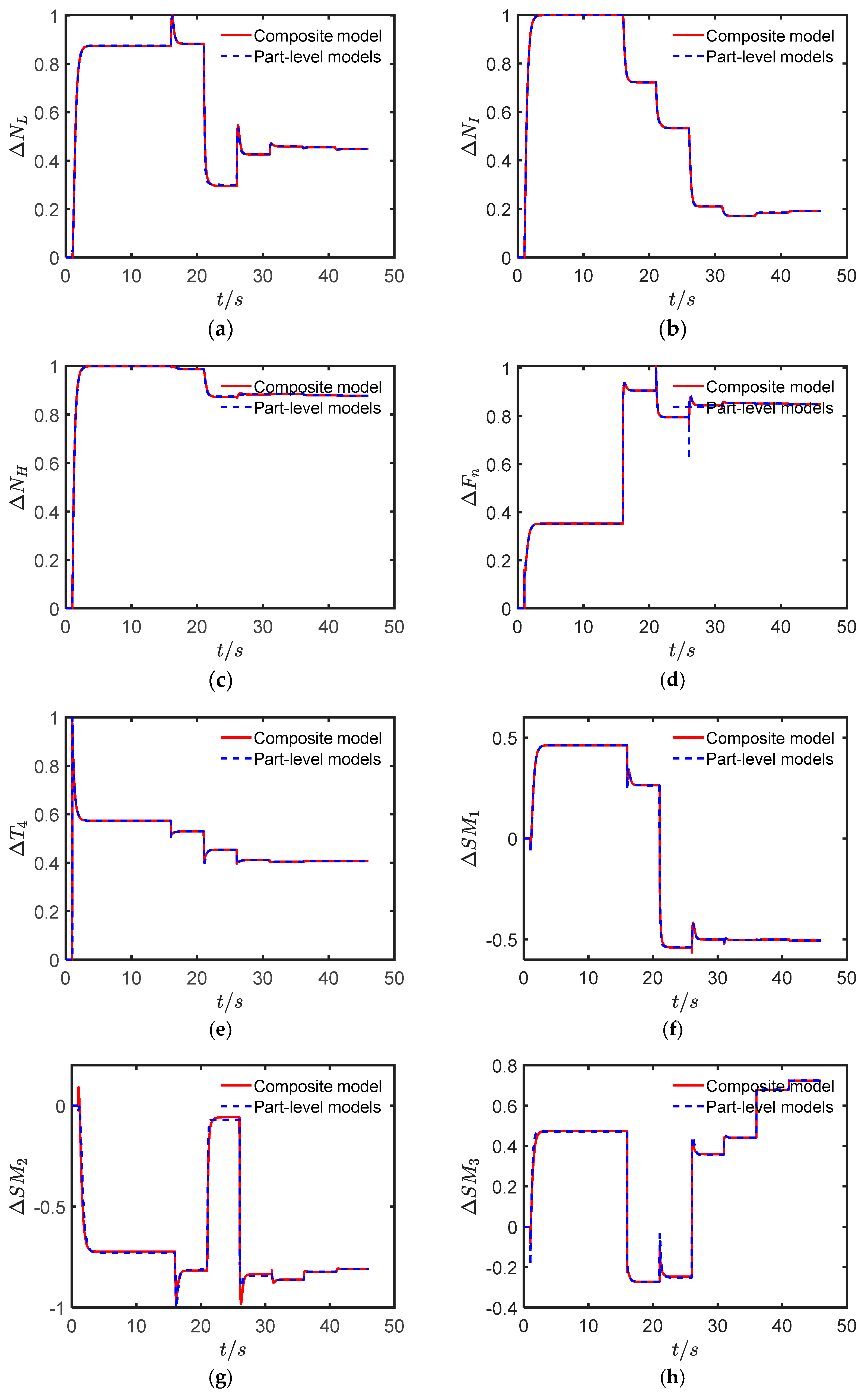
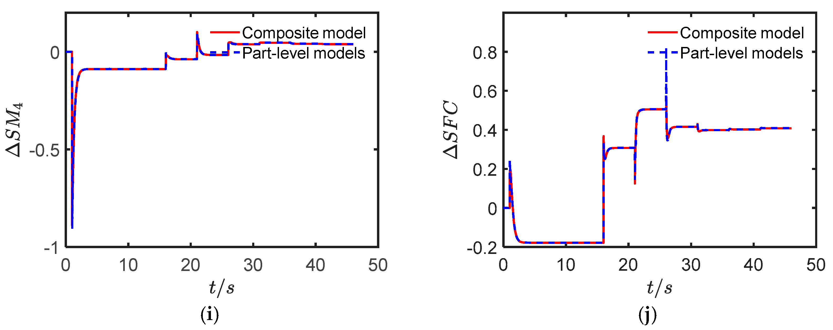
3.1. Composite Model’s Dynamic Accuracy

As can be seen from Figure 4, the modeling error between the composite model and the component-level model in the figure is basically negligible, which indicates that the composite model can meet the accuracy requirements of the dynamic simulation.

3.2. Optimization Results Based on PSM

As can be seen from Figure 5, the fuel consumption rate can be reduced by 2.6% in the minimum fuel consumption mode, which meets the expected requirements, but the thrust fluctuation, pre-turbine temperature, and speed are overshot. Therefore, a multivariable steady-state controller is designed based on MPC to meet the needs of engine optimization control mode switching.

3.3. MPC Controller Control Effect

As shown in Figure 7, the simulation results show that MPC can effectively suppress the thrust fluctuation phenomenon in the optimization process and significantly inhibit the overshoot problem of surge margin, which can realize the smooth transition of engine steady-state point switching.

4. Discussion

Compared with BPNN, the airborne composite model based on Kriging interpolation in this paper shows superior performance in the prediction of steady-state points of high-throughflow engines, which needs to be further studied, including the direct use of the Kriging model for nonlinear performance optimization, avoiding the linearization loss caused by the expansion into the PSM, and further improving the optimization accuracy.

Some scholars have proposed Explicit Model Predictive Control (EMPC) to convert the online calculation of MPC into an offline calculation. However, because the state quantity of the high-through-flow engine includes three speed quantities, the method of employing EMPC leads to more than 100 state partitions of a single steady-state point, which greatly increases the amount of offline computation so that it cannot be directly applied to aero-engine predictive control; therefore, it is a feasible strategy to reduce the model order using the method of model order reduction first, and then using the method of EMPC.

5. Conclusions

• In this paper, a new composite model modeling method is proposed, which uses the Kriging model to fit the strong nonlinear characteristics of the engine at the ground, sub-patrol, and over-patrol working points, expanding the PSM at the steady-state point to improve the real-time performance of the model.
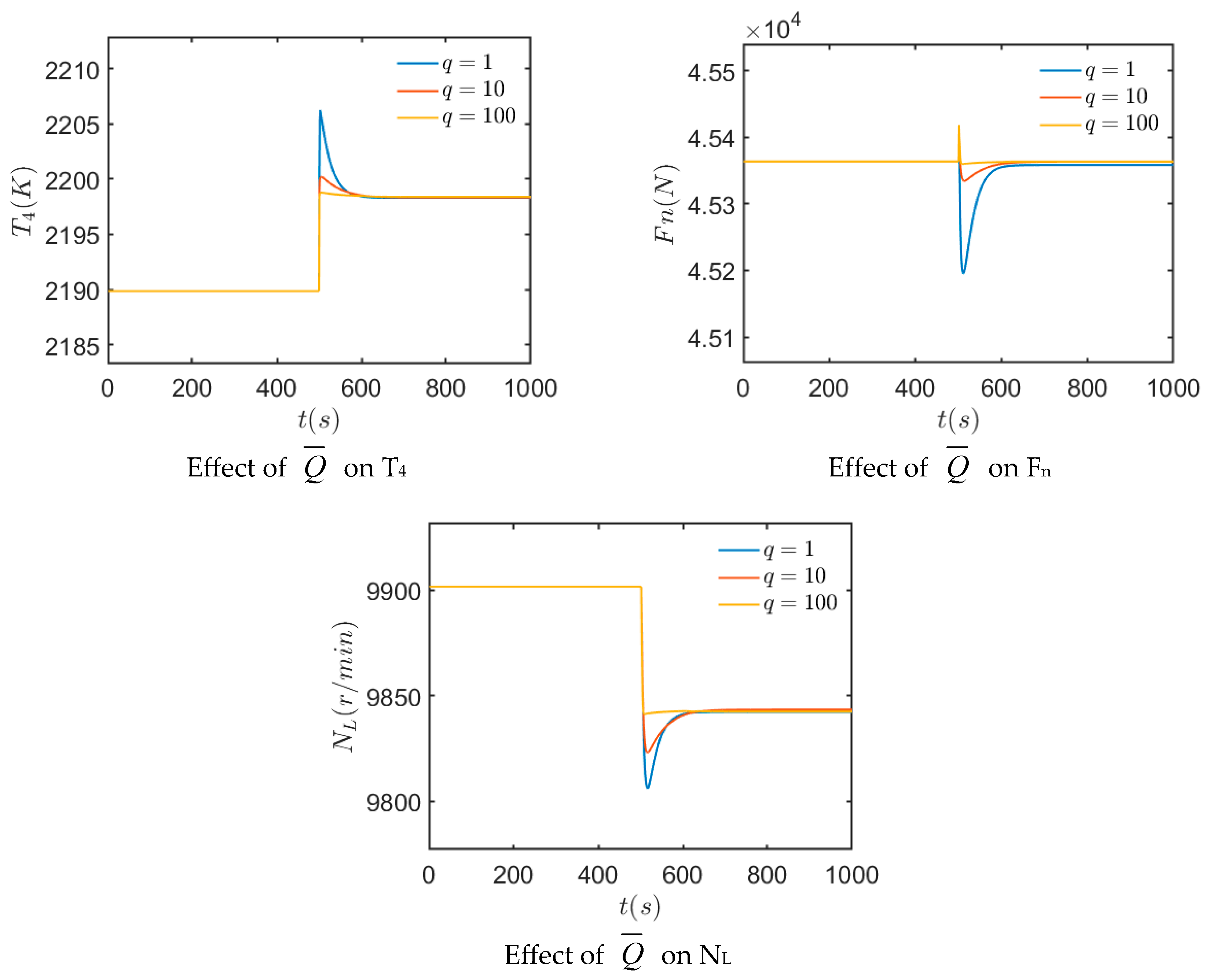
• Based on the linear optimization algorithm, the performance optimization problem of the engine is studied, and the optimization effect is studied by taking the over-cruise state as an example, and the results show that the fuel consumption rate in this state is significantly reduced
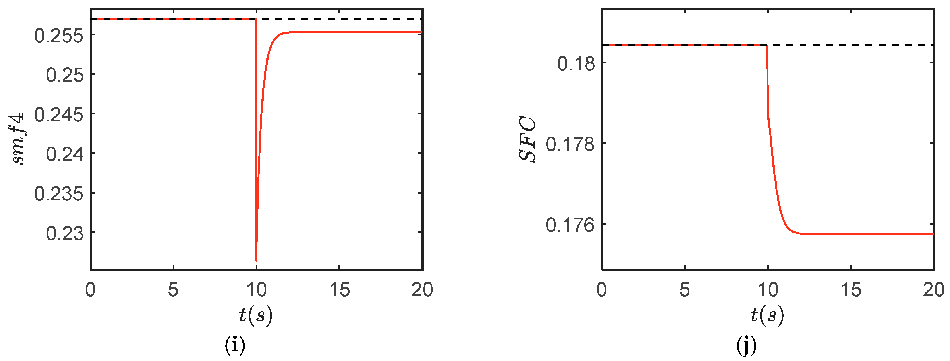
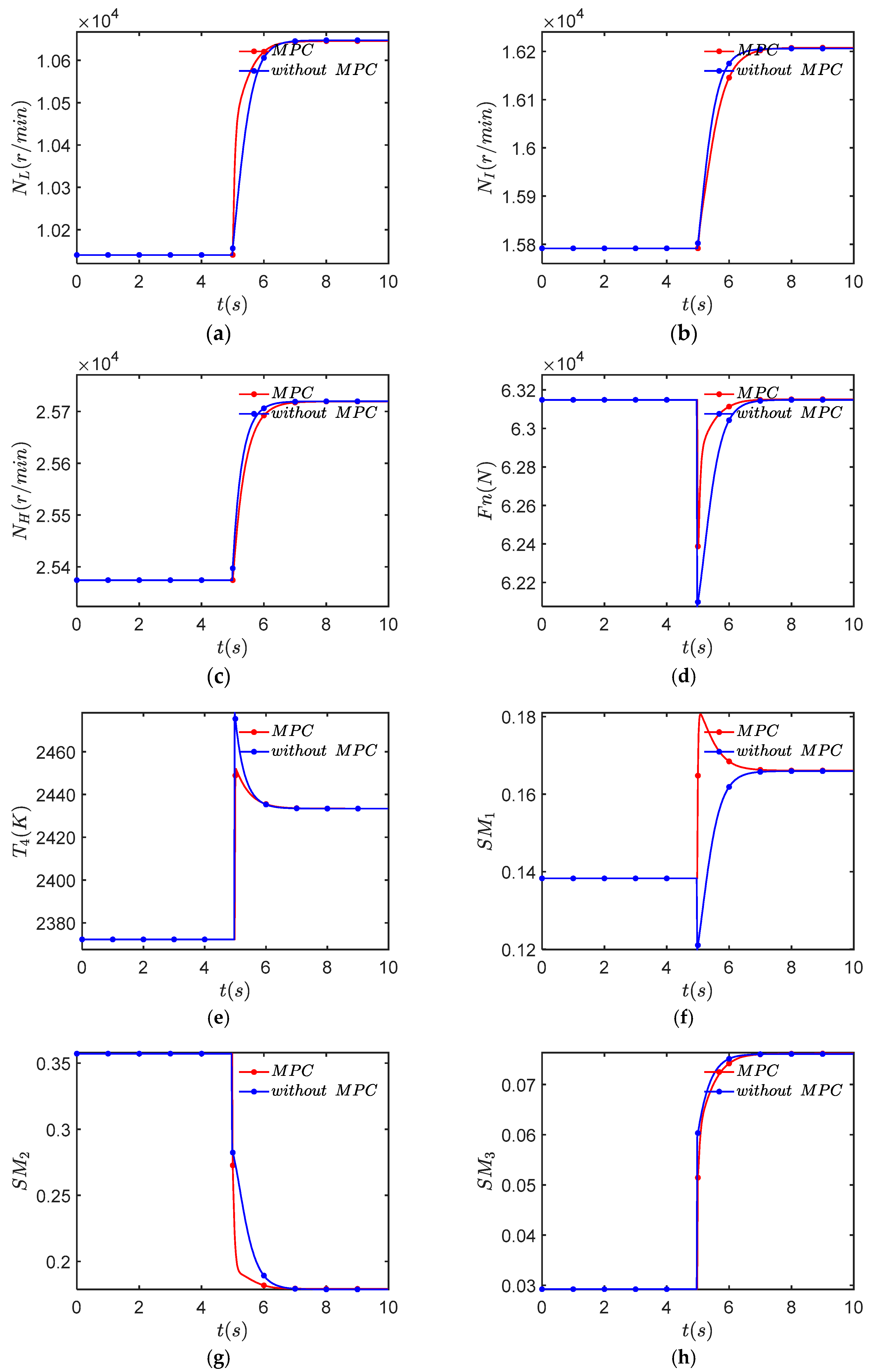
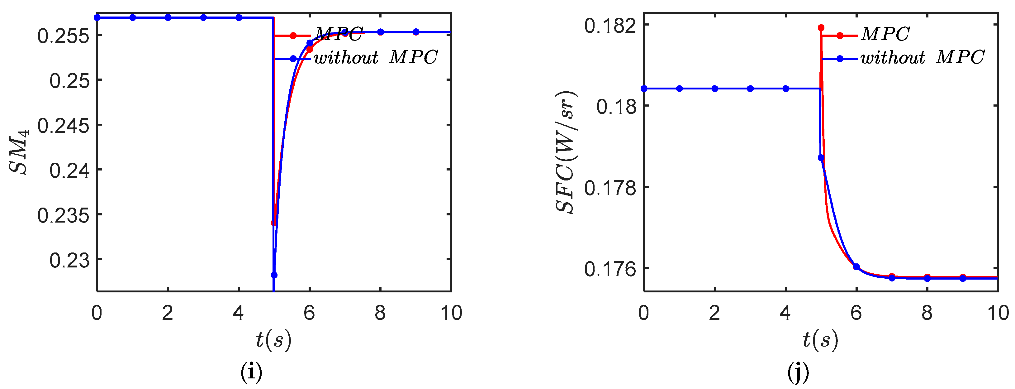
• In order to improve the response speed of the performance optimization control algorithm, a constraint protection method based on Model Predictive Control was studied. The results show that the temperature and surge margin overshoot problems are effectively suppressed in the minimum fuel consumption mode, which can make the engine work more safely.
• In order to solve the disadvantage of MPC with a large amount of online computation, some scholars have proposed Explicit Model Predictive Control (EMPC) to convert the online computation of MPC into offline computation. However, because the state quantity of the high-through-flow engine includes three speed quantities, the method of employing EMPC leads to more than 100 state partitions of a single steady-state point, which greatly increases the amount of offline computation so that it cannot be directly applied to aero-engine predictive control. Thus, it is a feasible strategy to reduce the model order by using the method of model order reduction first and then using the method of EMPC.

References

1. Pan, X.; Wang, X.; Wang, R.; Wang, L. Infrared radiation and stealth characteristics prediction for supersonic aircraft with uncertainty. Infrared Phys. Technol. 2015, 73, 238–250. [Google Scholar] [CrossRef]
2. Presz, W.; Nelson, C. Gas turbine exhaust cooling concepts. In Proceedings of the 30th Joint Propulsion Conference and Exhibit, Indianapolis, IN, USA, 27–29 June 1994. [Google Scholar]
3. Chen, H.; Zhang, H.; Xi, Z.; Zheng, Q. Modeling of the turbofan with an ejector nozzle based on infrared prediction. Appl. Therm. Eng. 2019, 159, 113910. [Google Scholar] [CrossRef]
4. Wang, F.; Ji, H.H.; Yu, M.F. Influence of total temperature and pressure at the inlet of convergent ex-haust system of turbofan engine on temperature distribution at plume centerline. J. Aerosp. Power 2016, 31, 816–822. [Google Scholar]
5. Liu, Y.B.; Xu, Z.G.; Ye, D.X.; Chen, H.; Zheng, Q.; Zhang, H. A Study on Performance Seeking Control of Minimum Infrared Characteristic Mode for Turbofan Engine. J. Propuls. Technol. 2020, 41, 10. (In Chinese) [Google Scholar]
6. Chen, H.; Zheng, Q.; Gao, Y.; Zhang, H. Performance Seeking Control of Minimum Infrared Characteristic on Double Bypass Variable Cycle Engine. Aerosp. Sci. Technol. 2020, 108, 106359. [Google Scholar] [CrossRef]
7. Xu, Z.G. Research on Cycling Parameter Optimization and Modeling Technology of Low Infrared Turbofan Engine. Master’s Thesis, Nanjing University of Aeronautics and Astronautics, Nanjing, China, 2020. [Google Scholar]
8. Wang, Z.X.; Song, F.; Zhou, L.; Zhang, X.B. Research Progress on Numerical Scaling Technology for Aero Engines. J. Propuls. Technol. 2018, 39, 1441–1454. [Google Scholar]
9. Shi, Y. Research on Full-State Performance Model of Civil Large-Bypass Ratio Turbofan Engine. Ph.D. thesis, Northwestern Polytechnical University, Xi’an, China, 2017. [Google Scholar]
10. Yu, B.; Shu, W.; Cao, C. A Novel Modeling Method for Aircraft Engine Using Nonlinear Autoregressive Exogenous (NARX) Models Based on Wavelet Neural Networks. Int. J. Turbo Jet Engines 2018, 35, 161–169. [Google Scholar] [CrossRef]
11. Dewei, X.; Qiangang, Z.; Haibo, Z.; Cheng, C.; Juan, F. Airborne adaptive steady-state model of aero engine based on NN-PSM. J. Aerodyn. 2022, 37, 409–423. [Google Scholar]
12. Zhu, J.; Liu, Y.; Luo, W.; Guo, F. Thrust-matching and optimization design of turbine-based combined cycle engine with trajectory optimization. Int. J. Turbo Jet-Engines 2024, 41, 719–729. [Google Scholar] [CrossRef]
13. Feng, J.; Tang, Y.; Zhu, S.; Deng, K.; Bai, S.; Li, S. Design of a combined organic Rankine cycle and turbo-compounding system recovering multigrade waste heat from a marine two-stroke engine. Energy 2024, 309, 133151. [Google Scholar] [CrossRef]
14. Qureshi, R.R.; Ford, D.N.; Wolf, C.M. Descriptive design structure matrices for improved system dynamics qualitative modeling. Syst. Dyn. Rev. 2024, 40, e1764. [Google Scholar] [CrossRef]
15. Schneider, S.J. Analysis of Turbine Blade Relative Cooling Flow Factor Used in the Subroutine Coolit Based on Film Cooling Correlations; National Aeronautics and Space Administration, Glenn Research Center: Cleveland, OH, USA, June 2015. [Google Scholar]
16. Qingxi, W.; Xiaobo, G. Particle swarm optimization algorithm based on Lévy flight. Comput. Appl. Res. 2016, 33, 2588–2591. [Google Scholar]
17. Wang, Y.; Liu, Y.; Wang, J.; Ma, L.; Cao, R.; Xu, Z. Optimization of aerospace engine bolt tightening based on Kriging model. Proc. Inst. Mech. Eng. 2024, 238, 9711–9725. [Google Scholar] [CrossRef]
18. Chen, J.; Zhang, C.; Chen, W.; Zhang, Z. Design and optimization of the exhaust system for an aviation piston engine. J. Phys. Conf. Ser. 2024, 2879, 012005. [Google Scholar] [CrossRef]
19. Huang, X.; Wang, P.; Wang, Q.; Zhang, L.; Yang, W.; Li, L. An improved adaptive Kriging method for the possibility-based design optimization and its application to aeroengine turbine disk. Aerosp. Sci. Technol. 2024, 153, 109495. [Google Scholar] [CrossRef]
20. Ghanbarpour, K.; Bayat, F.; Jalilvand, A. An MPC-based fault tolerant control of wind turbines in the presence of simultaneous sensor and actuator faults. Comput. Electr. Eng. 2024, 122, 109931. [Google Scholar] [CrossRef]
Figure 1. The structure of the engine.
Aerospace 12 00010 g001
Figure 2. Optimization process.
Aerospace 12 00010 g002
Figure 3. Diagram of steady-state characteristics. (a) Diagram of thrust characteristics. (b) Fuel consumption rate characteristic diagram. (c) Surge margin characteristic diagram.
Aerospace 12 00010 g003
Figure 4. Simulation results. (a) Simulation results of NL. (b) Simulation results of NI. (c) Simulation results of NH. (d) Simulation results of Fn. (e) Simulation results of T4. (f) Simulation results of SMF1. (g) Simulation results of SMF2. (h) Simulation results of SMF3. (i) Simulation results of SMF4. (j) Simulation results of SFC.
Aerospace 12 00010 g004aAerospace 12 00010 g004b
Figure 5. Optimism results of supersonic cruise. (a) Optimism results of NL. (b) Optimism results of NI. (c) Optimism results of NH. (d) Optimism results of Fn. (e) Optimism results of T4. (f) Optimism results of smf1. (g) Optimism results of smf2. (h) Optimism results of smf3. (i) Optimism results of smf4. (j) Optimism results of SFC.
Aerospace 12 00010 g005aAerospace 12 00010 g005b
Figure 6. The influence of the Q ¯ matrix element on the MPC result.
Aerospace 12 00010 g006
Figure 7. Comparison chart with or without MPC. (a) Comparison chart of NL. (b) Comparison chart of NI. (c) Comparison chart of NH. (d) Comparison chart of Fn. (e) Comparison chart of T4. (f) Comparison chart of smf1. (g) Comparison chart of smf2. (h) Comparison chart of smf3. (i) Comparison chart of smf4. (j) Comparison chart of SFC.
Aerospace 12 00010 g007aAerospace 12 00010 g007b